Embed Size (px)
Citation preview

Lectures onNumerical Methods For Non-Linear
Variational Problems
By
R. Glowinski
Tata Institute of Fundamental ResearchBombay
1980

Lectures onNumerical Methods For Non-Linear
Variational Problems
By
R. Glowinski
Notes by
G. Vijayasundaram
Adimurthi
Published for theTata Institute of Fundamental Research, Bombay
Springer-VerlagBerlin Heidelberg New York
1980

Author
R. GlowinskiUniversite Pierre et Marie Curie
Laboratoire d’Analyse Numerique 189Tour 55–65 5em etage
4, Place Jussieu75230 PARIS CEDEX 05
FRANCE
c© Tata Institute of Fundamental Research, 1980
ISBN 3-540-08774-5 Springer-Verlag, Berlin Heidelberg, New YorkISBN 0-387-08774-5 Springer-Verlag, New York. Heidelberg,. Berlin
No part of this book may be reproduced in anyform by print, microfilm or any other means with-out written permission from the Tata Institute ofFundamental Research, Colaba, Bombay 400 005
Printed by N.S. Ray at The Book Centre Limited Sion East, Bombay400 022 and Published by H. Goetze Springer-Verlag, Heidelberg,
West GermanyPrinted in India

To the memory ofG. Stampacchia

Preface
These notes correspond to a course of about fifteen lectures given atthe Tata Institute of Fundamental Research Centre, Indian Institute ofScience, Bangalore in January and February 1977.
The main goal of this course and of the corresponding notes istoprovide an introduction to the study of Nonlinear Variational Problems;they do not have pretention to cover all the aspects of this very importantsubject, since for example the Navier–Stokes equations fornewtonianincompressible viscous flows have not been considered here (we referfor this last problem to, e.g., TEMAM [1] and GIRAULT-RAVIART[1]).
Some questions pertinent to the main subject of these notes have notbeen treated here since they have been considered in the T.I.F.R. LectureNotes of P.G. CIARLET [1] and J.CEA [2].
Chapters 1 and 2 are concerned withElliptic Variational Inequali-tites (E.V.I.) more precisely with their approximation (mostly by finiteelement methods) and also their iterative solution. Several examples,coming from Mechanics illustrate the methods which are described inthese two chapters.
The following Chapter 3 is only an introduction to the approxima-tion of Parabolic Variational Inequalities (P.V.I.); we have however stud-ied with some details a particular P.V.I. related to the unsteady flow ofsome viscous plastic media (Bingham fluids) in a cylindricalpipe.
In Chapter 4 we show how Variational Inequalities concepts andmethods may be useful to study some Nonlinear Variational equations.
In Chapter 5 we discuss the iterative solution of some Variational
v

vi 0. Preface
Problems with a very specific structure allowing their solution by de-composition - coordination methods via augmented lagrangians; severaliterative methods are described and illustrated by examples, mostly fromMechanics.
In Chapter 6, which unlike the previous chapters is largely heuristi-cal, we show how some of the tools of the Chapters I–IV may be used tosolve numerically a difficult and important nonlinear problem of FluidDynamics: namely the steady transonic potential flow of an inviscidcompressible fluid. This last chapter is obviously just an introduction tothis very important and difficult subject.
I would like to thank all the people who make my stay in India amost enjoyable experience and more particularly Professors K.G. RA-MANATHAN, K. BALAGANGADHARAN and M.K.V. MURTHY.
These Notes were taken by M. ADIMURTHI and M.G. VIJAYA-SUNDARAM; I would like to thank them for their devoted efforts.
I would like to thank also S. KESAVAN and L. REINHART for theircareful reading of the proofs and the various improvements they havesuggested. Eventually I would like to express all my acknowledgementsto Mrs. F. WEBER for her beautiful typing of these Notes and toMr.M. Bazot who did all the artwork.
R. GlowinskiRocquencourt, France
November, 1979

Contents
Preface v
1 Generalities On Elliptic Variational... 11 Introduction . . . . . . . . . . . . . . . . . . . . . . . . 12 Functional Context . . . . . . . . . . . . . . . . . . . . 13 Existence And Uniqueness Results For EVI... . . . . . . 44 Existence And Uniqueness Results... . . . . . . . . . . . 75 -Internal Approximation of EVI of First Kind . . . . . . 126 Internal Approximation of EVI of Second Kind . . . . . 177 References . . . . . . . . . . . . . . . . . . . . . . . . . 21
2 Application of The Finite Element Method To... 231 Introduction . . . . . . . . . . . . . . . . . . . . . . . . 232 An Example of EVI of The First Kind:... . . . . . . . . . 243 A Second Example of EVI of The... . . . . . . . . . . . 424 A Third Example of EVI of The... . . . . . . . . . . . . 625 An Example of EVI of The Second Kind:... . . . . . . . 786 A Second Example of EVI of The... . . . . . . . . . . . 917 On Some Useful Formulae . . . . . . . . . . . . . . . . 114
3 On The Approximation of Parabolic Variational Inequaliti es1171 Introduction References . . . . . . . . . . . . . . . . . . 1172 Formulation And Statement of The Main Results . . . . 1173 Numerical Schemes For Parabolic Linear Equations . . . 1194 Approximation of PVI of The First Kind . . . . . . . . . 122
vii

viii Contents
5 Approximation of PVI of The Second Kind . . . . . . . 1236 Application to a Specific Example:... . . . . . . . . . . . 125
4 Applications of elliptic variational Inequality... 1331 Introduction . . . . . . . . . . . . . . . . . . . . . . . . 1332 Theoretical and Numerical Analysis of... . . . . . . . . . 1343 A Subsonic Flow Problem . . . . . . . . . . . . . . . . 167
5 Decomposition–Coordination methods by augmented... 1751 Introduction . . . . . . . . . . . . . . . . . . . . . . . . 1752 Properties of (P) And of The Saddle-Points... . . . . . . 1783 Description of The Algorithms . . . . . . . . . . . . . . 1814 Convergence of Alg 1 . . . . . . . . . . . . . . . . . . . 1835 Convergence of ALG 2 . . . . . . . . . . . . . . . . . . 1946 Applications . . . . . . . . . . . . . . . . . . . . . . . . 2007 General Comments . . . . . . . . . . . . . . . . . . . . 214
6 On the Computation of Transonic Flows 2151 Introduction . . . . . . . . . . . . . . . . . . . . . . . . 2152 Generalities . . . . . . . . . . . . . . . . . . . . . . . . 2153 Mathematical Model For The Transonic... . . . . . . . . 2174 Reduction to an Optimal Control Problem . . . . . . . . 2205 Approximation . . . . . . . . . . . . . . . . . . . . . . 2226 Iterative Solution of The Approximate Problems . . . . . 2307 A Numerical Experiment . . . . . . . . . . . . . . . . . 2358 Comments Conclusion . . . . . . . . . . . . . . . . . . 238

Chapter 1
Generalities On EllipticVariational Inequalities AndOn Their Approximation
1 Introduction
An important and very useful class of non-linear problems arising from 1
mechanics, physics etc. consists of the so-called Variational Inequali-ties. We mainly consider the following two types of variational inequal-ities, namely
1. Elliptic Variational Inequalities (EVI),
2. Parabolic Variational Inequalities (PVI).
In this chapter (following LIONS-STAMPACCHIA 1) we shall re-strict our attention to the study of the existence, uniqueness and approx-imation of the solutions of EVI.
2 Functional Context
In this section we consider two classes of EVI, namely EVI of the firstkind and EVI of the second kind.
1

2 1. Generalities On Elliptic Variational...
2.1 Notations
• V : real Hilbert space with scalar product (·, ·) and associatednorm‖ · ‖.
• V∗ : the dual space ofV.
• a(·, ·) : V × V → R is a bilinear, continuous andV -elliptic formon V × V.
A bilinear forma(·, ·) is said to beV -elliptic if there exists a positiveconstantα such thata(v, v) ≥ α ‖ v ‖2 ∀v ∈ V.
In general we do not assumea(·, ·) to be symmetric, since in someapplications non-symmetric bilinear forms may occur naturally (see forinstance COMINCIOLI [1]).
• L : V → R continuous, linear functional.
• K is a closed, convex, non-empty subset ofV.
• j(·) : V → R = R∪∞ is a convex, lower semi -continuous (l.s.c.) and proper functional
( j(·) is proper if j(v) > −∞∀v ∈ V and j . ∞).
2.2 EVI of first kind
To find u∈ V such that u is a solution of the problem2
(P1)
a(u, v− u) ≥ L(v− u),∀v ∈ K,
u ∈ K.
2.3 EVI of second kind
To find u∈ V such that u is a solution of the problem
(P2)
a(u, v− u) + j(v) − j(u) ≥ L(v− u)∀v ∈ V,
u ∈ V.

2. Functional Context 3
2.4 Remarks:
REMARK 2.1. The cases above considered are the simplest and mostimportant. LIONS and BENSOUSSAN [1] considered some generaliza-tion of problem(P1) called Quasi Variational Inequalities(QVI) whicharises for instance from Decision Sciences. A typical problem of QVI is:
To findu ∈ V such thata(u, v− u) ≥ L(v− u)∀v ∈ K(u),
u ∈ K(u)
where v→ K(v) is a family of closed, convex non-empty subsets of V.
REMARK 2.2. If K = V and j ≡ 0 then the problems(P1) and (P2)reduce to the classical variational equation
a(u, v) = L(v) ∀v ∈ V,
u ∈ V.
REMARK 2.3. The distinction between(P1) and (P2) is artificial, for 3
(P1) can be considered as a particular case of(P2) by replacing j(·) in(P2) by the indicator function IK of K defined by
IK(v) =
0 if v ∈ K
+∞ if v < K.
Even though (P1) is a particular case of (P2) it is worthwhile con-sidering (P1) separately because it arises in a natural way and we willget geometrical insight into the problem.
Exercise 2.1.Prove that IK is a convex, l.s.c. and proper functional.
Exercise 2.2. Show that(P1) is equivalent to the problem of findingu ∈ V such that a(u, v− u) + IK(v) − IK(u) ≥ L(v− u)∀v ∈ V.

4 1. Generalities On Elliptic Variational...
3 Existence And Uniqueness Results For EVI ofFirst Kind
3.1 A Theorem of existence and uniqueness
THEOREM 3.1. (LIONS-STAMPACCHIA 1).The problem (P1) hasone and only one solution
Proof. (I)Uniqueness:Let u1 andu2 be solutions of (P1). We have then
a(u1, v− u1) ≥ L(v− u1) ∀v ∈ K, u1 ∈ K, (3.1)
a(u2, v− u2) ≥ L(v− u2) ∀v ∈ K, u2 ∈ K. (3.2)
Puttingu2 for v in (3.1) andu1 for v in (3.2) and adding we get, byusing theV -ellipticity of a(·, ·),
α ‖ u2 − u1 ‖2≤ a(u2 − u1, u2 − u1) ≤ 0
which provesu1 = u2 sinceα > 0.(2) ExistenceWe use a generalization of the proof used by CLARLET [1] for4
proving the Lax-Milgram Lemma, i. e. we will reduce the problem (P1)to afixed pointproblem.
By the Riesz representation theorem for Hilbert space thereexistA ∈ L (V,V)(A = At if a(·, ·) is symmetric) andℓ ∈ V such that
(Au, v) = a(u, v) ∀u, v ∈ V andL(v) = (ℓ, v) ∀v ∈ V. (3.3)
Then the problem (P1) is equivalent to findingu ∈ V such that
(u− ρ(Au− ℓ) − u, v− u) ≤ 0 ∀v ∈ K,
u ∈ K, ρ > 0.
(3.4)

3. Existence And Uniqueness Results For EVI... 5
This is equivalent to findingu such that
u = PK(u− ρ(Au− ℓ)), for someρ > 0, (3.5)
wherePK denotes the projection operator fromV to K in the‖ · ‖ norm.Consider the mapWρ : V → V defined by
Wρ(v) = PK(v− ρ(Av− ℓ)). (3.6)
Let v1, v2 ∈ V. Then sincePK is a contraction we have
‖Wρ(v1) −Wρ(v2) ‖2≤‖ v2 − v1 ‖2 +ρ2 ‖ A(v2 − v1 ‖2
−2ρa(v2 − v1, v2 − v1).
Hence we have
‖Wρ(v1) −Wρ(v2) ‖2≤ (1− 2ρα + ρ2 ‖ A ‖2) ‖ v2 − v1 ‖2 . (3.7)
ThusWρ is a strict contraction mapping if 0< ρ <2α
‖ A ‖2. By taking
ρ in this range we have a unique solution for the fixed point problemwhich implies the existence of a solution for (P1).
3.2 Remarks
REMARK 3.1. If K = V, Theorem 3.1 reduces to Lax-Milgram Lemma5(see CIARLET [1]).
REMARK 3.2. If a(·, ·) is symmetric then Theorem 3.1 can be provedusing optimization methods (see CEA [1]).
Let J : V → R be defined by
J(v) =12
a(v, v) − L(v). (3.8)
Then

6 1. Generalities On Elliptic Variational...
(i) lim‖v‖→+∞
J(v) = +∞
sinceJ(v) =12
a(v, v) − L(v) ≥α
2‖ v ‖2 − ‖ L ‖‖ v ‖.
(ii) J is strictly convex.
SinceL is linear, to prove the strict convexity ofJ it suffices toprove that
v→ a(v, v)
is strictly convex. Let 0< t < 1 andu, v ∈ V with u , v;0 < a(v− u, v− u) = a(u, u) + a(v, v) − 2a(u, v). Hence we have
2a(u, v) < a(u, u) + a(v, v). (3.9)
Using (3.9) we have
a(tu+ (1− t)v, tu+ (1− t)v) =
t2a(u, u) + 2t(1− t)a(u, v) + (1− t)2a(v, v) <
< ta(u, u) + (1− t)a(v, v).(3.10)
Thereforea(v, v) is strictly convex.
(iii) Since a(·, ·) andL are continuous,J is continuous.6
From these properties ofJ and standard results of Optimization The-ory (cf. CEA [1]) it follows that the minimization problem offinding usuch that
(π)
J(u) ≤ J(v) ∀v ∈ K,
u ∈ K
has one and only one solution. Therefore (π) is equivalent to the problemof finding u such that
(J′(u), v− u) ≥ 0 ∀v ∈ K,
u ∈ K,
(3.11)

4. Existence And Uniqueness Results... 7
where J′(u) is the Gateaux derivativeof J at u. Since (J′(u), v) =a(u, v) − L(v) we see that (P1) and (π) are equivalent ifa(·, ·) is sym-metric.
Exercise 3.1.Prove that(J′(u), v) = a(u, v)− L(v) ∀u, v∈ V and hencededuce that J′(u) = Au∼ ℓ ∀u ∈ V.
REMARK 3.3. The proof of Theorem 3.1 given a natural a naturalalgorithm for solving(P1) since v→ PK(v− ρ(Av− ℓ)) is acontraction
mapping for0 < ρ <2α
‖ A ‖2. Hence we can use the following algorithm
to find u:Let u0 ∈ V, (3.12)
un+1 = PK(un − ρ(Aun − ℓ)). (3.13)
Then un → u strongly in V whereu is the solution of (P1). Inpractice it is not easy to calculateℓ and A unlessV = V∗. To projectoverK may be as difficult as solving (P1). In general this method cannotbe used for computing the solution of (P1) if K , V (at least not sodirectly).
We observe that ifa(·, ·) is symmetric thenJ′(u) = Au− ℓ and hence 7
(3.13) becomesun+1 = PK(un − ρ(J′(un)). (3.13’)
This method is know as theGradient -Projectionmethod.
4 Existence And Uniqueness Results For EVI ofSecond Kind
THEOREM 4.1. (LIONS-STAMPACCHIA [1]) Problem(P2) has oneonly one solution.
Proof. As in Theorem 3.1 we shall first prove uniqueness and then ex-istence
(1) Uniqueness.Let u1 andu2 be two solutions of (P2). Then wehave
a(u1, v− u1) + j(v) − j(u1) ≥ L(v− u1) ∀v ∈ V, u1 ∈ V, (4.1)

8 1. Generalities On Elliptic Variational...
a(u2, v− u2) + j(v) − j(u2) ≥ L(v− u2) ∀v ∈ V, u2 ∈ V, (4.2)
Since j(·) is a proper map there existsv0 ∈ V such that−∞ < j(v0) <∞. Hence fori = 1, 2
−∞ < j(ui) ≤ j(v0) − L(v0 − ui) + a(ui , v0 − ui). (4.3)
This shows thatj(ui ) is finite for i = 1, 2. Hence by substitutingu2
for v in (4.1) andu1 for v in (4.2) and adding we obtain
α ‖ u1 − u2 ‖2≤ a(1−u2, u1 − u2) ≤ 0. (4.4)
Henceu1 = u2.(2) Existence. For eachu ∈ V andρ > 0 we associate a problem
(πuρ) of type (P2) defined as below :
To find w∈ V such that
(πuρ)
(w, v− w) + ρ j(v) − ρ j(w)
≥ (u, v− w) + ρL(v− w) − ρa(u, v− w) ∀v ∈ V,
w ∈ V.(4.5)
The advantage of considering this problem over the problem (P2)8
is that the bilinear form associated with (πuρ) is the inner product ofV
which is symmetric.Let us first assume that (πu
ρ) has a unique solution for allu ∈ V andρ > 0. For eachρ define the mapfρ : V → V by fρ(u) = w wherew isthe unique solution of (πu
ρ).We shall show thatfρ is a uniformly strict contraction mapping for
suitable chosenρ.Let u1, u2 ∈ V andwi = fρ(ui), i = 1, 2. Sincej(·) is proper we have
j(ui) finite which can be proved as in (4.3). Therefore we have
(w1,w2 − w1) + ρ j(w2) − ρ j(w1)
≥ (u1,w2 − w1) + ρL(w2 − w1) − ρa(u1,w2 − w1), (4.6)

4. Existence And Uniqueness Results... 9
(w2,w1 − w2) + ρ j(w1) − ρ j(w2)
≥ (u2,w1 − w2) + ρL(w1 − w2) − ρa(u2,w1 − w2). (4.7)
Adding these inequalities we obtain
‖ fρ(u1) − fρ(u2) ‖2 =‖ w2 − w1 ‖2
=≤ ((I − ρA)(u2 − u1),w2 − w1)
=≤‖ I − ρA ‖ ‖ u2 − u1 ‖ ‖ w2 − w1 ‖ .
(4.8)
Hence‖ fρ(u1) − fρ(u2) ‖≤‖ I − ρA ‖ ‖ u2 − u1 ‖
It is easy to show that‖ I − ρA ‖< 1 when 0< ρ <2α‖ A ‖2
. This
proves thatfρ is uniformly a strict contracting mapping and hence hasa unique fixed pointu. This u turns out to be the solution of (P2) sincefρ(u) = u implies (u, v − u) + ρ j(v) − ρ j(u) ≥ (u, v − u) + ρL(v − u) −ρa(u, v− u) ∀v ∈ V. Therefore
a(u, v− u) + j(v) − j(u) ≥ L(v− u) ∀v ∈ V. (4.9)
Hence (P2) has a unique solution.The existence and uniqueness of the problem (πu
ρ) follows from thefollowing
Lemma 4.1. Let b : V × V → R be a symmetric continuous, bilinear, V9
-elliptic form with V -elliptic constantβ. Let L∈ V∗ and j : V → R be a
convex, l.s.c. proper functional. Let J(v) =12
b(v, v) + j(v) − L(v). Then
the minimization problem(π):To findu such that
(π)
J(u) ≤ J(v) ∀v ∈ V,
u ∈ V

10 1. Generalities On Elliptic Variational...
has a unique solution which is characterised by
b(u, v− u) + j(v) − j(u) ≥ L(v− u) ∀v ∈ V,
u ∈ V.
(4.10)
Proof. (i) Existence and uniqueness of uSinceb(·, ·) is strictly convex,j is convex andL is linear, we haveJ
strictly convex. J is l.s.c. becauseb(·, ·) andL are continuous andj isl.s.c.
Since j is convex, l.s.c. and proper, there existsλ ∈ V∗ andµ ∈ Rsuch that
j(v) ≥ λ(v) + µ (cf. EKLAND - TEMAM [1]) ,
therefore
J(v) ≥ β2 ‖ v ‖2 − ‖ λ ‖‖ v ‖ − ‖ L ‖ ‖ v ‖ +µ
=
(√β2 ‖ v ‖ − (‖λ‖+‖L‖)
2
√2β
)2
+ µ − (‖λ‖+‖L‖)2
2β .
(4.11)
HenceJ(v)→ +∞ as ‖ v ‖→ +∞. (4.12)
Hence (cf. CEA [1] ) there exists a unique solution for the optimiza-10
tion problem (π).Characterisation of u : We show that the problem (π) is equivalent
to (4.10) and thus get a characterisation ofu.(2) Necessity of(4.10) : Let 0< t ≤ 1. Letu be the solution of (π).
Then for allv ∈ V we have
J(u) ≤ J(u+ t(v− u)). (4.13)
SetJ0(V) =12
b(v, v) − L(v), then (4.13) becomes
0 ≤ J0(u+ t(v− u)) − J0(u) + j(u+ t(v− u)) − j(u)
≤ J0(u+ t(v− u)) − J0(u) + t[ j(v) − j(u)] ∀v ∈ V
(4.14)

4. Existence And Uniqueness Results... 11
got by using convexity ofj. Dividing by t in (4.14) and taking the limitast → 0 we get
0 ≤ (J′0(u), v− u) + j(v) − j(u) ∀v ∈ V. (4.15)
Sinceb(·, ·) is symmetric we have
(J′0(v),w) = b(v,w) − L(w) ∀v,w ∈ V. (4.16)
From (4.15) and 4.16 we obtain
b(u, v− u) + j(v) − j(u) ≥ L(v− u) ∀v ∈ V.
This proves the necessity.(3) Sufficiency of (4.10). Letu be a solution of (4.10) ; forv ∈ V
J(v) − J(u) =12
[b(v, v) − b(u, u)] + j(v) − j(u) − L(v− u). (4.17)
But
b(v, v) = b(u+ v− u, u+ v− u)
= b(u, u) + 2b(u, v− u) + b(u− v, u− v).
Therefore 11
J(v)− J(u) = b(u, v−u)+ j(v)− j(u)−L(v−u)+12
b(v−u, v−u). (4.18)
Sinceu is a solution of (4.10) andb(v− u, v− u) ≥ 0 we get
J(v) − J(u) ≥ 0. (4.19)
Henceu is a solution of (π).By takingb(·, ·) to be the inner product inV and replacingj(v) and
L(v) in Lemma 4.1 byρ j(v) and (u, v) + ρL(v) − ρa(u, v), respectively,we get the solution for (πu
ρ).
12 1. Generalities On Elliptic Variational...
REMARK 4.1. From the proof of Theorem 4.1 we get an algorithm forsolving(P2). This algorithm is given by
(1) u0 ∈ V, 0 < ρ < 2α‖A‖
2,
(2) (un+1, v− un+1) + ρ j(v) − ρ j(un+1) ≥ (un, v− un+1)
+ρL(v− un+1) − ρa(un, v− un+1) ∀v ∈ V,
(3) un+1 ∈ V.
(4.20)
Then one can easily see thatun → u stronglyin V andu will be thesolution of (P2). Difficulties may arise in using this scheme whenj(·)is not assumed to be differentiable. At each iteration the problem wehave to solve is also a problem of the same order of difficulty as that ofthe original problem (actually conditioning can be better providedρ hasbeen conveniently chosen). Ifa(·, ·) is not symmetric the fact that (·, ·) issymmetric can also give some simplification.
5 -Internal Approximation of EVI of First Kind
5.1 Introduction
In this chapter we shall study the approximation of EVI of thefirst kindfrom an abstract, axiomatic point of view.
5.2 The continuous problem
The assumptions onV, K, L anda(·, ·) are as in section 2. We are inter-12
ested in the approximation of
(P1)
a(u, v− u) ≥ L(v− u) ∀v ∈ K,
u ∈ K,
which has one and only solution by Theorem 3.1.

5. -Internal Approximation of EVI of First Kind 13
5.3 The approximate problem
5.3.1 The approximation ofV and K
We are given a parameterh converging to 0 and a family (Vh)h of closedsubspaces ofV. (In practiceVh are finite dimensional and the parameterh varies over a sequence). We are also given a family (Kh)h of closed,convex, non-empty subsets ofV with Kh ⊂ Vh ∀h (in general we do notassumeKh ⊂ K) such that (Kh)h satisfies the following two conditions :
(i) If ( vh)h is such thatvh ∈ Kh ∀h and (vh)H is bounded inV then theweakcluster points of (vh)h belong toK.
(ii) Assume there existχ ⊂ V, χ = K and rh : χ → Kh such thatlimh→0
rhv = v strongly inV, ∀v ∈ χ.
REMARK 5.1. If Kh ⊂ K ∀h then (i) is trivially satisfied because K isweakly closed.
REMARK 5.2. ∩hKh ⊂ K.
REMARK 5.3. A useful variant of condition (ii) for rh is (ii)’ Assumethere exists a subsetχ ⊂ V such thatχ = K and rh : χ → Vh with theproperty that for each v∈ χ, there exists h0 = h0(v) with rhv ∈ Kh for allh ≤ h0(v) and lim
h→0rhv = v stronglyin V.
5.3.2 Approximation of (P1):
The problem (P1) is approximated by
(P1h)
a(uh, vh − uh) ≥ L(vh − uh) ∀vh ∈ Kh,
uh ∈ Kh.
THEOREM 5.1. (P1h) has a unique solution. 13
Proof. In Theorem 3.1 takingV to beVh andK to beKh we have theresult.

14 1. Generalities On Elliptic Variational...
REMARK 5.4. In most of the cases it will be necessary to replace a(·, ·)and L by ah(., .) and Lh (usually defined - in practical cases - from a(·, ·)and L by a Numerical Integration procedure). Since there is nothingvery new on that matter compared to the classical linear case, we shallsay nothing about this problem for which we refer to CIARLET [1, Chap.8].
5.4 Convergence results
THEOREM 5.2. With the above assumptions on K and(Kh)h we havelimh→0‖ uh − u ‖V= 0 with uh the solution of(P1h) and u the solution of
(P1).
Proof. In this kind of convergence we usually divide the proof into threeparts. First we obtain a priori estimates for (uh)h, then weak convergenceof (uh)h and finally with the help of weak convergence, we will provestrong convergence.
(1) Estimation for uh.We will now show that there exist constantsC1 andC2 independent
of h such that‖ uh ‖2≤ C1 ‖ uh ‖ +C2,∀h. (5.1)
Sinceuh is the solution of (P1h) we have
a(uh, vh − uh) ≥ L(vh − uh)∀vh ∈ Kh (5.2)
i.e.a(uh, uh) ≤ a(uh, vh) − L(vh − uh).
By V -ellipticity we get
α ‖ uh ‖2≤‖ A ‖ · ‖ uh ‖ · ‖ vh ‖ + ‖ L ‖ (‖ vh ‖ + ‖ u− h ‖) ∀vh ∈ Kh.
(5.3)Let v0 ∈ χ andvh = rhv0 ∈ Kh. By condition (ii) onKh we have
rhv0 → v0 strongly inV and hence‖ vh ‖ is uniformly bounded by aconstantm. Hence (5.3) can be written as
‖ uh ‖2≤1α(m ‖ A ‖ + ‖ L ‖) ‖ uh ‖ + ‖ L ‖ m = C1 ‖ uh ‖ +C2,

5. -Internal Approximation of EVI of First Kind 15
whereC1 =1α
(m ‖ A ‖ + ‖ L ‖) andC2 =mα‖ L ‖; then (5.1) implies 14
‖ uh ‖≤ C ∀h.
(2) Weak convergence of(uh)h : Relation (5.1) givesuh is uniformlybounded. Hence there exists a subsequence sayuhi such thatuhi con-verges tou∗ weakly inV. By condition (i) on (Kh)h we haveu∗ ∈ K. Wewill prove thatu∗ is a solution for (P1). We have
a(uhi , uhi ) ≤ a(uhi , vhi ) − L(vhi , uhi ) ∀vhi ∈ Khi . (5.4)
Let v ∈ χ andvhi = rhi v. Then (5.4) becomes
a(uhi , uhi ) ≤ a(uhi , rhi v) − L(rhi v− uhi ). (5.5)
Since rhi v converges strongly tov and uhi converges tou∗ weakly ashi → 0 taking the limit in (5.5) we get
lim infhi→0
a(uhi , uhi ) ≤ a(u∗, v) − L(v− u∗) ∀v ∈ χ. (5.6)
Also we have
0 ≤ a(uhi − u∗, uhi − u∗) ≤ a(uhi , uhi ) − a(uhi , u∗) − a(u∗, uhi ) + a(u∗, u∗)
i. e.a(uhi , u
∗) + a(u∗, uhi ) − a(u∗, u∗) ≤ a(uhi , uhi ).
By taking the limit we obtain
a(u∗, u∗) ≤ lim infhi→0
a(uhi , uhi ). (5.7)
From (5.6) and (5.7) we get
a(u∗, u∗) ≤ lim infhi→0
a(uhi , uhi ) ≤ a(u∗, v) − L(v− u∗) ∀v ∈ χ.
Therefore we have, 15
a(u∗, v− u∗) ≥ L(v− u∗) ∀v ∈ χ,
u∗ ∈ K.
(5.8)

16 1. Generalities On Elliptic Variational...
Sinceχ is dense inK anda(·, ·), L are continuous, we get from (5.8)
a(u∗, v− u∗) ≥ L(v− u∗) ∀v ∈ K,
u∗ ∈ K.(5.9)
Henceu∗ is a solution of (P1). By Theorem 3.1, the solution for (P1)is unique and henceu∗ = u is the unique solution. Henceu is the onlycluster point ofuhh in the weak topology ofV. Hence the wholeuhhconverges tou weakly.
(3) Strong convergence: We have byV−ellipticity of a(·, ·)
0 ≤ α ‖ uh−u ‖2≤ a(uh−u, uh−u) = a(uh, uh)−a(uh, u)−a(u, uh)+a(u, u)(5.10)
whereuh is the solution of (P1h) andu is the solution of (P1). Sinceuh
is the solution of (P1h) andrhv ∈ Kh for anyv ∈ χ, we get by (P1h)
a(uh, uh) ≤ a(uh, rhv) − L(rhv− uh) ∀v ∈ χ. (5.11)
Since limh→0
uh = u weaklyin V and limh→0
rhv = v stronglyin V (by condition
(ii)) we obtain, from (5.10), (5.11) and after taking the lim, that∀v ∈ χwe have:
0 ≤ α lim inf ‖ uh − u ‖2≤ α lim sup ‖ uh − u ‖2≤ a(u, v− u) − L(v− u).(5.12)
By densityandcontinuity, (5.12) also holds∀v ∈ K; then takingv = uin (5.12) we obtain that
limh→0‖ uh − u ‖2= 0
i.e. the strong convergence.
REMARK 5.5. Error estimates for the EVI of the first kind can be found16
in FALK [1], [2], [3], STRANG-MOSCO [1], STRANG [1], GLOWIN-SKI-LIONS-TREMOLIERES (G.L.T.) [1], [2], CIARLET [1], BREZZI[1], FALK-MERCIER [1], GLOWINSKI [1]. But like in many nonlinearproblems the methods used to obtain these estimates are specific to the

6. Internal Approximation of EVI of Second Kind 17
particular problem under consideration (as we shall see in the followingsections).
This remark still holds for the approximation of EVI of the secondkind which is the subject of Section 6.
REMARK 5.6. If for a given problem, several approximations areavailable, and if computations are needed, the choice of theapproxi-mations to be used is not obvious. We have to take into accountnot onlythe convergence properties of the method, but also the computation in-volved in that method. Some iterative methods are best suited only forsome problems. Some methods are easier to program than others.
6 Internal Approximation of EVI of Second Kind
6.1 The Continuous Problem
The assumptions onV, a(·, ·), L j(·) being as in Section 2.1, we shallconsider the approximation of
(P2)
a(u, v− u) + j(v) − j(u) ≥ L(v− u) ∀v ∈ V,
u ∈ V
which has one and only one solution by Theorem 4.1.
6.2 Definition of the approximate problem
Preliminary remark : We assume in the sequel thatj : V → R iscontinuous. We can prove the same sort of results as in this sectionunder less restrictions (see Chapter 4, Section 2).
6.2.1 Approximation of V
Given a real parameterh converging to 0 and a family (Vh)h of closed 17
subspaces ofV (in practice we will takeVh to be finite dimensional andh to vary over a sequence), we assume that (Vh)h satisfies

18 1. Generalities On Elliptic Variational...
(i) there existsU ⊂ V such thatU = V and for eachh, a maprh :U → Vh such that lim
h→0rhv = v strongly inV, ∀v ∈ U.
6.2.2 Approximation of j(·)
We approximate the functionalj(·) by ( jh)h where for eachh, jhsatisfies
jh : Vh→ R
jhis convex, l.s.c. and uniformly proper in h.
(6.1)
The family (jh)h is said to beuniformly proper in hif there existλ ∈ V∗ andµ ∈ R such that
h(vh) ≥ λ(vh) + µ ∀vh ∈ Vh,∀h. (6.2)
Furthermore we assume that (jh)h satisfies
(ii) if vh→ v weaklyin V then
lim infh→0
jh(vh) ≥ j(v)
(iii) limh→0
jh(rhv) = j(v) ∀v ∈ U.
REMARK 6.1. In all the applications we know, if j(·) is a continuousfunctional then it is always possible to construct continuous jh satisfying(ii) and (iii).
REMARK 6.2. In some cases we are fortunate enough to have jh(vh) =j(vh)∀vh, ∀h, and then (ii) and (iii) are trivially satisfied.
6.2.3 Approximation of (P2)
We approximate (P2) by18
(P2h)
a(uh, vh − uh) + jh(vh) − jh(uh) ≥ L(vh − uh) ∀vh ∈ Vh,
uh ∈ Vh.

6. Internal Approximation of EVI of Second Kind 19
THEOREM 6.1. Problem (P2h) has one only one solution.
Proof. In Theorem 4.1 takingV to be Vh, j(·) to be jh(·) we get theresult.
REMARK 6.3. Remark 5.4 of Section 5 still holds for(P2) and(P2h).
6.3 Convergence results
THEOREM 6.2. Under the above assumptions on(Vh)h and ( jh)h wehave
limh→0‖ uh − u ‖= 0,
limh→0
jh(uh) = j(u).(6.3)
Proof. As in the proof of Theorem 5.2 we divide the proof into threeparts.
(1) Estimation for uh. We will show that there exist positive con-stantsC1 andC2 independent ofh such that
‖ uh ‖2≤ C1 ‖ uh ‖ +C2 ∀h. (6.4)
Sinceuh is the solution of (P2h) we have
a(uh, uh) + jh(uh) ≤ a(uh, vh) + jh(vh) − L(vh − uh) ∀vh ∈ Vh. (6.5)
By using relation (6.2) we get
α ‖ uh ‖2≤‖ λ ‖ ‖ uh ‖ + |µ|+ ‖ A ‖ ‖ uh ‖ ‖ vh ‖+ | jh(vh)|+ ‖ L ‖ (‖ vh ‖ + ‖ uh ‖). (6.6)
Letv0 ∈ U andvh = rhv0. By using condition (i) and (iii) there existsa constantm, independent ofh such that‖ vh ‖≤ m and | jh(vh)| ≤ m.Therefore (6.6) can be written as
‖ uh ‖2 ≤ 1α (‖ λ ‖ + ‖ A ‖ ·m+ ‖ L ‖) ‖ uh ‖ +m
α (1+ ‖ L ‖) + |µ|α
= C1 ‖ uh ‖ +C2

20 1. Generalities On Elliptic Variational...
where 19
C1 =1α
(‖ λ ‖ + ‖ A ‖ ·m+ ‖ L ‖) and C2 =mα
(1+ ‖ L ‖) +|µ|α
and (6.4) implies
‖ uh ‖≤ C ∀h whereC is a constant.
(2) Weak convergence ofuh: Relation (6.4) gives thatuh is uni-formly bounded. Therefore there exists a subsequence (uhi )hi such thatuhi → uh weakly inV.
Sinceuh is the solution of (P1h) andrhv ∈ Vh ∀h and∀v ∈ U we get
a(uhi , uhi ) + jhi (uhi ) ≤ a(uhi , rhi v) + jhi (rhvi) − L(rhi v− uhi ). (6.7)
By condition (iii) and weak convergence ofuhi we get
lim infh→0
[a(uhi , uhi )+ jhi (uhi )] ≤ a(u∗, v) + j(v) − L(v− u∗) ∀v ∈ U. (6.8)
As in (5.7) and using condition (ii), we get
a(u∗, u∗) + j(u∗) ≤ lim infh→0
[a(uhi , uhi ) + jhi (uhi )]. (6.9)
From (6.8), (6.9) and using the density ofU we have
a(u∗, v− u∗) + j(v) − j(u∗) ≥ L(v− u∗) ∀v ∈ V,
u∗ ∈ V.
This impliesu∗ is a solution of (P2). Henceu∗ = u is the unique solutionof (P2) and this shows that (uh) converges to uweakly.
(3) Strong convergence of(uh)h: We have byV -ellipticity of a(·, ·)20
and by (P2h)
α ‖ uh − u ‖2 + jh(uh) ≤ a(uh − u, uh − u) + jh(uh) =
= a(uh, uh) − a(u, uh) − a(uh, u) + a(u, u) + jh(uh) ≤≤ a(uh, r − hv) + jh(rhv) − L(rhv− uh) − a(u, uh)
−a(uh, u) + a(u, u) ∀v ∈ U.(6.10)

7. References 21
The right hand side of inequality (6.10) tends toa(u, v− u) + j(v) −L(v− u) ash→ 0∀v ∈ U. Therefore we have
lim inf h→0 jh(uh) ≤ lim inf h→0[α ‖ uh − u ‖2 + jh(uh)] ≤
≤ lim suph→0[α ‖ uh − u ‖2 + jh(uh)] ≤
≤ a(u, v− u) + j(v) − L(v− u)∀v ∈ U.
(6.11)
By density ofU, (6.11) holds∀v ∈ V. Replacingv by u in (6.11) andusing condition (ii) we obtain
j(u) ≤ lim infh→0
jh(uh) ≤ lim suph→0
[α ‖ u− uh ‖2 + jh(uh)] ≤ j(u).
This implies that
limh→0
jh(uh) = j(u) and
limh→0‖ uh − u ‖= 0.
This proves the theorem.
7 References
For generalities on variational inequalities from a theoretical point of 21
view see Lions-Stampacchia [1], Lions [1], Ekeland-Temam [1].For generalities on the approximation of variational inequalitiesfrom
the numerical point of view see Falk [1], Glowinski-Lions-Tremolieres[1], [2], Strang [1], Brezzi-Hager-Raviart [1].


Chapter 2
Application of The FiniteElement Method To TheApproximation of SomeSecond Order EVI
1 Introduction
In this chapter we consider some examples of EVI of the first and sec- 22
ond kinds. These EVI are related to second order partial differentialoperators (for fourth order problems see GLOWINSKI [2]). The Phys-ical Interpretation and some properties of the solution aregiven. Finiteelement approximations of these EVI are considered and convergenceresults are proved. In some particular cases we prove error estimates.
Some of the results in this chapter may be found in G.L.T. [1],[2].For the approximation of the EVI of first kind by the finite element meth-ods we refer also to FALK [1], STRANG [1], MOSCO-STRANG [1],CIARLET [1], BREZZI-HAGER-RAVIART [1].
We also deal with iterative methods for solving the correspondingapproximate problems (cf. CEA [1], G.L.T. [1], [2]).
23
24 2. Application of The Finite Element Method To...
2 An Example of EVI of The First Kind: The Ob-stacle Problem
Notations 1. All the properties of Sobolev spaces used in this chapterare proved in LIONS [2], NECAS [1]. Usually we shall have
• Ω: a bounded domain inR2
• Γ : ∂Ω
• x = x1, x2 a generic point ofΩ
• ∇ = ∂
∂x1,∂
∂x2
• Cm(Ω): space of m -times continuously differentiable real valuedfunctions for which all the derivatives up to order m are continu-ous inΩ,
• Cm0 (Ω) = v ∈ Cm(Ω) : Supp(v) is a compact subset ofΩ.
• ‖ v ‖m,p,Ω=∑|α|≤m
‖ Dαv ‖Lp(Ω) for v ∈ Cm(Ω) whereα = (α1, α2);23
α1, α2 non-negative integers,|α| = α1 + α2 and Dα =∂|α|
∂xα11 ∂xα2
2
.
• Wm,p(Ω) : completion of Cm(Ω) in the norm defined above.
• Wm,p(Ω): completion of Cm0 (Ω) is the above norm
• Hm(Ω) =Wm,2(Ω),
• Hm0 (Ω) =Wm,2(Ω),
D(Ω) = C∞0 (Ω).

2. An Example of EVI of The First Kind:... 25
2.1 The continuous problem:
LetV = H1
0(Ω) = v ∈ H1(Ω) : v|Γ = trace de v surΓ = 0
(cf. LIONS [2], NECAS[1]).
a(u, v) =∫
Ω
∇u.∇vdx
where
∇u.∇v =∂u∂x1
∂v∂x1+∂u∂x2
∂v∂x2
.,
L(v) = 〈 f , v〉 for f ∈ V∗ = H−1(Ω) andv ∈ V. LetΨ ∈ H1(Ω) ∩C0(Ω)andΨ|Γ ≤ 0. DefineK = v ∈ H1
0(Ω) : v ≥ Ψa.e. onΩ.Then the obstacle problem is a (P1) problem defined by :Find u such that
a(u, v− u) ≥ L(v− u)∀v ∈ K,
u ∈ K.(2.1)
The physical interpretation of this problem is the following: let anelastic membrane occupy a regionΩ in the x1, x2 plane; this membraneis fixed along the boundaryΓ of Ω. When there is no obstacle, from thetheory of elasticity the vertical displacementu, obtained by applying avertical forceF, is given by the Dirichlet problem
−∆u = f in Ω,
u|Γ = 0(2.2)
where f = F/t, t being the tension. 24
When there is an obstacle, we have a free boundary problem andthe displacementu satisfies the variational inequality (2.1) withΨ be-ing the height of the obstacle. Similar EVI also occur, sometimes withnon-symmetric bilinear forms, in mathematical models for the followingproblems:
• Lubrication phenomena (cf. CRYER [1]).

26 2. Application of The Finite Element Method To...
• Filtration of liquids in porous media (cf. BAIOCCHI [1], COM-INCIOLI [1]),
• Two dimensional, irrotational flows of perfect fluids (cf. BREZISSTAMPACCHIA [1], BREZIS [1], CLAVLDINI-TOURNEMINE[1]).
• Wake problems (cf. BOURGAT- DUVAUT [1]).
2.2 Existence and uniqueness results:
For proving the existence and uniqueness of the problem (2.1), we needthe following lemmas stated below without proof (for proof of the lem-mas, see for instance LIONS [1], NECAS [1], STAMPACCHIA [1]).
Lemma 2.1. LetΩ be a bounded domain inRN. Then the semi-normon H1(Ω)
v→(∫
Ω
|∇v|2dx
)1/2
is a norm on H10(Ω) and it is equivalent to the norm on H10(Ω) induced
from H1(Ω).
The above Lemma 2.1 is known as Poincare-Friedrichs lemma.
Lemma 2.2(STAMPACCHIA [1]). Let f : R → R be uniformly Lips-chitz continuous (i.e.∃k > 0 such that| f (t) − f (t′)| ≤ k|t − t′| ∀t, t′ ∈ R)and such f′ has a finite number of points of discontinuity. Then the in-duced map f∗ on H1(Ω) defined by u→ f (u) is a continuous map intoH1(Ω). Similar results holds for H10(Ω) when ever f(0) = 0.
COROLLARY 2.1. If v+ and v− denote the positive and the negative25
parts of v for v∈ H1(Ω) (respectively H10(Ω)) then the map v→ v+, v−is continuous from H1(Ω) → H1(Ω) × H1(Ω) (respectively H10(Ω) →H1
0(Ω) × H10(Ω)). Also v→ |v| is continuous.
THEOREM 2.1. Problem (2.1) has a unique solution.

2. An Example of EVI of The First Kind:... 27
Proof. In order to apply Theorem 3.1 of Chapter 1 we have to prove that(., .) is V-elliptic and thatK is a closed, convex, non-empty set.
TheV-ellipticity of a(., .) follows from Lemma 2.1 and the convexityof K is trivial; then
(1) K is non-empty. We have
Ψ ∈ H1(Ω) ∩C0(Ω) with Ψ ≤ 0 onΓ.
Hence, by Corollary 2.1,Ψ+ ∈ H1(Ω). SinceΨ|Γ ≤ 0 we haveΨ+|Γ = 0. This impliesΨ+ ∈ H1
0(Ω); then
Ψ+ = maxΨ, 0 ≥ Ψ
ThusΨ+ ∈ K. HenceK is non-empty.
(2) K is closed. Let vn → v strongly in H10(Ω) wherevn ∈ K and
v ∈ H10(Ω). Hencevn → v strongly in L2(Ω). Therefore we can
extract a subsequencevni such thatvni → v a.e. onΩ. Thenvni ≥ Ψ a.e. onΩ implies that
v ≥ Ψ a.e. onΩ;
thereforev ∈ K.
Hence, by Theorem 3.1 of Chapter 1, We have a unique solutionfor (2.1).
2.3 Interpretation of (2.1) as a free boundary problem
For the solutionu of (2.1) we define 26
Ω+ = x : x ∈ Ω, u(x) > Ψ(x)Ω0 = x : x ∈ Ω, u(x) = Ψ(x)γ = ∂Ω+ ∩ ∂Ω0; u+ = u|Ω+ ; u0 = u|Ω0.

28 2. Application of The Finite Element Method To...
Classically the problem (2.1) has been formulated as the problem offinding γ (the free boundary)andu such that
− ∆u = f onΩ+, (2.3)
u = Ψ onΩ0, (2.4)
u = 0 onΓ, (2.5)
u+|γ = u0|γ (2.6)
The physical interpretation of these relations is the following: (2.3)means that onΩ+ the membrane is strictly over the obstacle; (2.4) meansthat onΩ0 the membrane is in contact with the obstacle; (2.6) is trans-mission relation at the free boundary.
Actually (2.3)–(2.6) are not sufficient to characteristicu since thereare an infinity of solutions for (2.3)–(2.6). Therefore it isnecessary toadd other transmission properties: for instance, ifΨ is smooth enough(sayΨ ∈ H2(Ω)), we require the continuity of∇u at γ (we may ask∇u ∈ H1(Ω) × H1(Ω)).
REMARK 2.1. This kind of free boundary interpretation holds for sev-eral problems modelled by EVI of first kind and second kind.
2.4 Regularity of solutions
We state without proof the following regularity theorem forthe problem(2.1).
THEOREM 2.2. (BREZIS- STAMPACCHIA [1]). LetΩ be a boundeddomain inR2 with a smooth boundary. If
L(v) =∫
Ω
f v dx with f ∈ Lp(Ω), 1 < p < ∞ (2.7)
andΨ ∈W2,p(Ω), (2.8)
then the solution of the problem(2.1) is in W2,p(Ω).27

2. An Example of EVI of The First Kind:... 29
REMARK 2.2. LetΩ ⊂ RN have a smooth boundary. We know that
Ws,p(Ω) ⊂ Ck(Ω) if s >Np+ k (2.9)
(cf. NECAS [1]). It follows that the solution u of(2.1)will be in C1(Ω)if f ∈ Lp(Ω), Ψ ∈ WP2, p(Ω) with p > 2 (take s= 2, N = 2, k = 1 in(2.9)).
The proof of this regularity result will be given in the followingsimple case:
L(v) =∫
Ω
f vdx, f ∈ L2(Ω), (2.10)
Ψ = 0 onΩ. (2.11)
Before proving that (2.10), (2.11) implyu ∈ H2(Ω), we shall recall aclassical lemma (also very useful in the analysis of fourth order prob-lems).
Lemma 2.3. Let Ω be a bounded domain ofRN with a boundaryΓsufficiently smooth. Then‖ ∆v ‖L2(Ω) defines a norm on H2(Ω) ∩ H1
0(Ω)which is equivalent to the norm induced by the H2(Ω)- norm.
Exercise 2.1.Prove the above Lemma 2.3 using the following regularityresult due to AGMON-NIRENBERG [1]:
If w ∈ L2(Ω) and ifΓ is smooth then the Dirichlet problem−∆v = w inΩ,
v|Γ = 0,
has a unique solution in H10(Ω)∩H2(Ω) (this regularity result also holdsif Ω is a convex domain withΓ Lipschitz continuous) .
We shall now apply the Lemma 2.3 to prove the following theoremusing a method of BREZIS-STAMPACCHIA [2].
THEOREM 2.3. If Γ is smooth enough,Ψ = 0 and L(v) =∫Ω
f vdx 28
with f ∈ L2(Ω) then the solution u of the problem(2.1)satisfiesu ∈ K ∩ H2(Ω),
‖ ∆u ‖L2(Ω)≤‖ f ‖L2(Ω) .(2.12)

30 2. Application of The Finite Element Method To...
Proof. From Theorem 2.1 it follows that problem (2.1) has a uniquesolution u, with L andΨ as above. Let∈> 0, consider the followingDirichlet problem
− ∈ ∆uǫ + uǫ = u in Ω,
uǫ |Γ = 0.(2.13)
Problem (2.13) has a unique solution inH10(Ω) and the smoothness
of Γ assures thatuǫ belongs toH2(Ω). Sinceu ≥ 0 a.e. onΩ, by themaximum principle for second order elliptic differential operators, (cf.MECAS [1]) we haveuǫ ≥ 0. Hence
uǫ ∈ K. (2.14)
From (2.14) and (2.1) we obtain
a(u, uǫ − u) ≥ L(uǫ − u) =∫
Ω
f (uǫ − u)dx. (2.15)
TheV-ellipticity of a(., .) implies
a(uǫ , uǫ − u) = a(uǫ − u, uǫ − u) + a(u, uǫ − u) ≥ a(u, uǫ − u),
so that,
a(uǫ , uǫ − u) ≥∫
Ω
f (uǫ − u)dx. (2.16)
By (2.13) and (2.16) we obtain
∈∫
Ω
∇uǫ .∇(∆uǫ ) dx≥∈∫
Ω
f∆uǫ dx
so that,29 ∫
Ω
∇uǫ .∇(∆u∈)dx≥∫
Ω
∆uǫdx. (2.17)
By Green’s formula, (2.17) implies
−∫
Ω
(∆uǫ )2dx≥
∫
Ω
f∆uǫdx.

2. An Example of EVI of The First Kind:... 31
Thus
‖ ∆u∈ ‖L2(Ω)≤‖ f ‖L2(Ω), (2.18)
usingSchwarz inequalityin L2(Ω). By Lemma 2.3 and relations (2.13),(2.18) we obtain
lim∈→0
uǫ = u weaklyinH2(Ω), (2.19)
(which implies that limuǫ = u strongly inHs(Ω), for everys < 2 (cf.NECAS [1])), so thatu ∈ H2(Ω) with
‖ ∆u ‖L2(Ω)≤‖ f ‖L2(Ω) . (2.20)
2.5 Finite Element Approximations of (2.1)
Henceforth we shall assume thatΩ is a polygonal domain ofR2. Con-sider a “ classical” triangulationCh ofΩ, i.e.Ch is a finite set of trianglesT such that
T ⊂ Ω∀T ∈ C + h,⋃
T∈Ch
T = Ω. (2.21)
T01 ∩ T0
2 = Ψ∀T1,T2 ∈ Ch and T1 , T2. (2.22)
Moreover∀T1, T2 ∈ Ch and T1 , T2, exactly one of the followingconditions must hold
(1) T1 ∩ T2 = Ψ
(2) T1 andT2 have only one common vertex,
(3) T1 andT2 have only a whole common edge.
(2.23)
30
As usualh will be the length of the largest edge of the triangles inthe triangulation.
From now on we restrict ourselves to piecewise linear and piecewisequadratic finite element approximations.
32 2. Application of The Finite Element Method To...
2.5.1 Approximation of V and K.
• Pk: space of polynomials inx1 andx2 of degree less than or equalto k.
• Σh = P ∈ Ω : P is a vertex ofT ∈ Ch
• Σ0h = P ∈ Σh : P < Γ.
• Σ′h = P ∈ Ω : P is the mid point of an edge ofT ∈ Ch.
• Σ′0h = P ∈ Σ′h : P < Γ.
• Σ1h = Σh andΣ2
h = Σh ∪ Σ′h.
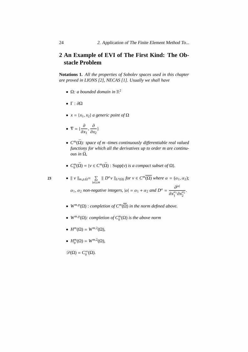
Figure 2.1 illustrates some further notations associated with an ar-bitrary triangleT. we havemiT ∈ Σ′h, MiT ∈ Σh. The centroid of thetriangleT is denoted byGT .
Figure 2.1:
The spacev = H10(Ω) is approximated by the family of subspaces31
(Vkh)h with k = 1 or 2 where
Vkh =
vh ∈ C0(Ω) : vh
∣∣∣Γ= 0 and vh
∣∣∣T∈ Pk ∀T ∈ Ch
.k = 1, 2.
2. An Example of EVI of The First Kind:... 33
It is clear thatVkh are finite dimensional (cf. CIARLET [1]). It is then
quite natural to approximateK by
Kkh =
vh ∈ Vk
h : vh(P) ≥ Ψ(p) ∀P ∈ Σkh
, k = 1, 2.
Proposition 2.1. The Kkh for k = 1, 2 are closed, convex, non-empty
subsets of Vkh.
Exercise 2.2.Prove Proposition 2.1.
2.5.2 The approximate problems
Fork = 1, 2 the approximate problems are defined by
(Pk1h)
a(uk
h, vh − ukh) ≥ L(vh − uk
h)∀vh ∈ Kkh,
ukh ∈ Kk
h.
From Theorem 3.1 of Chapter 1 and Proposition 2.1, it followsthat
Proposition 2.2. (Pk1h) has a unique solution for k= 1 and 2.
REMARK 2.3. If the bilinear form a(·, ·) is symmetric,(Pk1h) is actu-
ally equivalent to (cf. Chap. 1, Remark 3.2) thequadratic programmingproblem
minvh∈Kk
h
[12
a(vh, vh) − L(vh)
]. (2.24)
2.6 Convergence results
In other to simplify the convergence proof we shall assume inthis sectionthat
Ψ ∈ C0(Ω) ∩ H1 and Ψ ≤ 0 in a neighbourhood ofΓ. (2.25)
Before proving the convergence results we shall give two important 32
numerical quadrature schemes which will be used to prove theconver-gence theorem.

34 2. Application of The Finite Element Method To...
Exercise 2.3.With notations as in Fig.2.1, prove the following identitiesfor any triangle T
∫
Twdx=
meas.(T)3
3∑
i=1
w(MiT )∀w ∈ P1. (2.26)
∫
Twdx=
meas.(T)3
3∑
i=1
w(miT )∀w ∈ P2. (2.27)
Formula (2.26) is called theTrapezoidal Ruleand (2.27) is known asSimpson’s Integral formula. These formulae, not only have theoreticalimportance but also practical utility.
We have the following results about the convergence ofukh (solutions
of the problem (Pkh)) ash→ 0.
THEOREM 2.4. Suppose that the angles of the triangles ofCh areuniformly bounded below byθ0 > 0 as h→ 0; then for k= 1, 2
limh→0‖ uk
h − u ‖H10(Ω)= 0 (2.28)
where ukh and u are respectively the solutions of Pk1h and (2.1).
Proof. In this proof we shall use the followingdensity result to beproved later:
D(Ω) ∩ K = K. (2.29)
To prove (2.28) we shall use Theorem 5.2 of Chap. 1. To do this wehave to verify that the following two properties hold (fork = 1, 2):
(i) If ( vh)h is such thatvh ∈ Kkh ∀hand converges weakly tovash→ 0,
thenv ∈ K.
(ii) There existsχ, χ = K and rkh : χ → Kk
h such that limh→0
rkhv = v
=strongly in V ∀v ∈ χ.

2. An Example of EVI of The First Kind:... 35
Verification of (i).Using the notations of Fig.2.1 and consideringφ ∈33
D(Ω) with φ ≥ 0, we defineφh by φh =∑
T∈Ch
φ(Gt)χT whereχT is the
characteristic functionof T andGT is the centroid ofT. It is easy to seefrom the uniform continuity ofφ that
limh→0= φ strongly in L∞(Ω). (2.30)
Then we approximateΨ byΨh such thatΨh ∈ C0(Ω),Ψh|T ∈ Pk∀T ∈ Ch,
Ψh(P) = Ψ(P)∀P ∈ Σkh.
(2.31)
This functionΨh satisfies
limh→0Ψh = Ψ strongly in L∞(Ω). (2.32)
Let us consider a sequence (vh)h, vh ∈ Kkh ∀h such that
limh→0
vh = v weakly in V.
Then limh→o
vh = v strongly in L2(Ω), (cf. NECAS [1]) which, using
(2.30) and (2.32), implies that
limh→0
∫
Ω
(vh − Ψh)Ψhdx=∫
Ω
(v− Ψ)φdx, (2.33)
(actually sinceφh→ φ stronglyin L∞(Ω) the weak convergence ofvh inL2(Ω) is enough to prove (2.33)).
We have∫
Ω
(vh − φh)φhdx=∑
T∈⊂h
φ(Gt)∫
T(vh − Ψh)dx. (2.34)
From (2.26). (2.27) and the definition ofΨh we obtain for allT ∈ Ch.
∫
T(vh − Ψh)dx=
meas.(T)3
3∑
i=1
[vh(MiT ) − Ψh(MiT )] if k = 1, (2.35)

36 2. Application of The Finite Element Method To...
∫
T(vh − Ψh)dx=
meas.(T)3
3∑
i=1
[vh(miT ) − Ψh(miT )] if k = 2, (2.36)
34
Using the fact thatφh ≥ 0, the definition ofKkh and the relations
(2.35), (2.36) it follows from (2.34) that∫
Ω
(vh − Ψh)φh dx≥ 0∀φ ∈ D(Ω), φ ≥ 0,
so that ash→ 0 ∫
Ω
(v− Ψ)φdx≥ 0∀φ ∈ D(Ω), φ ≥ 0
which in turn impliesv ≥ Ψ a.e. inΩ. Hence (i) is verified.
Verification of (ii). From (2.29) it is natural to takeχ = D ∩ K. Wedefinerk
h : H10(Ω) ∩C0(Ω)→ Vk
h as the “ linear ” interpolation operatorwhenk = 1 and “ quadratic” interpolation operator whenk = 1, i.e.
rkhv ∈ Vk
h ∀v ∈ H10(Ω) ∩C0(Ω),
(rkhv)(p) = v(p)∀P ∈
∑kh for k = 1, 2.
(2.37)
On the one hand it is known (cf. for instance CIARLET [1], [2] ,STRANG-FIX [1]) that under the assumptions made onCh in statementof Theorem 2.4 we have
‖ rkhv− v ‖v≤ C hk ‖ v ‖Hk+1(Ω) ∀v ∈ D(Ω), k = 1, 2.
with C independent ofh andv . This implies that
limh→0‖ rk
hv− v ‖v= 0∀ ∈ χ, k = 1, 2.
On the other hand it is obvious that
rkhv ∈ Kk
h ∀v ∈ K ∩C0(Ω).
so that35
rkhv ∈ Kk
h ∀v ∈ χ, for k = 1, 2.
In conclusion with the aboveχ and rkh, (ii) is satisfied. Hence we
have proved the Theorem 2.4 modulo the proof of the density result(2.29).

2. An Example of EVI of The First Kind:... 37
Lemma 2.4. Under the assumptions(2.25)we haveD(Ω) ∩ K = K.
Proof. Let us prove the Lemma in two steps.
Step 1. Let us show that
K = v ∈ K ∩C0(Ω) : vcompact support inΩ (2.38)
is dense in K.
Let v ∈ K, K ⊂ H10(Ω) implies that exists a sequenceφnn in D(Ω)
such thatlimn→∞
φn = v strongly in V.
Definevn byvn = max(ψ, φn) (2.39)
so that
vn =12
[(Ψ + φn) + |Ψ − φn|].
Sincev ∈ K, from Corollary 2.1 and relations (2.39) i follows that
limn→∞
vn =12
[(Ψ + v) + |Ψ − v|] = max(Ψ, v) = v strongly in V. (2.40)
From (2.25) and (2.39) it follows that
each vn has a compact support inΩ, (2.41)
vn ∈ K ∩C0(Ω). (2.42)
From (2.40) - (2.42) we obtain (2.38) 36
Step 2. Let us show that
D(Ω) ∩K is denseK . (2.43)
This proves from Step 1, thatD(Ω) ∩ K is dense inK. Let ρn be asequence of mollifiers, i.e.
ρn ∈ D(R2), ρn ≥ 0,∫R2 ρn(y)dy = 1∞⋂
n=1Suppρn = 0, Suppρnis a decreasing sequence.
(2.44)

38 2. Application of The Finite Element Method To...
Let v ∈ K . Let v extension ofv defined by
v(x) =
v(x) if x ∈ Ω,0 if x < Ω,
thenv ∈ H1(R2). Let vn = v ∗ ρn i.e.
vn(x) =∫
R2ρn(x− y)v(y)dy (2.45)
then
vn ∈ D(R2),
Suppvn ⊂ Suppv+ Suppρ′nlimn→∞
vn = v strongly inH1(R2).
(2.46)
Hence from (2.41) and (2.46) we have
Supp(vn) ⊂ Ω for n large enough. (2.47)
We also have (since Supp(˜v)is bounded)37
lim vn = v strongly in L∞(R2). (2.48)
Definevn = vn|Ω, then (2.46)–(2.48) imply
vn ∈ D(Ω)
limn→∞
vn = v strongly in H10(Ω) ∩C0(Ω);
(2.49)
v ∈ K andΨ ≤ 0 in a neighbourhood ofΓ imply that there exists aδ > 0 such that
v = 0,Ψ ≤ 0 on Ωδ (2.50)
whereΩδ = x ∈ Ω : d(x, Γ) < δ.From (2.48) and (2.50) it follows that∀ ∈> 0, there exists ann0 =
n0(∈) such that∀n ≥ n0(∈)v(x)− ∈≤ vn(x) ≤ (x)+ ∈ ∀x ∈ Ω −Ωδ/2vn(x) = v(x) = 0 for x ∈ Ωδ/2
(2.51)

2. An Example of EVI of The First Kind:... 39
SinceΩ − Ωδ/2 is a compact subset ofΩ there exists a functionsθ (cf.for instanceH. CARTAN [1]) such that
θ ∈ D(Ω), θ ≥ 0 in Ω
θ(x) = 1∀x ∈ Ω −Ωδ/2(2.52)
Finally definewǫn = vn+ ∈ θ.
Then from (2.49), (2.51) and (2.52) we have
wǫn ∈ D(Ω)
lim∈→0n→∞
n≥n0(∈)
wǫn = v strongly in H1
0(Ω),
with wǫn(x) ≥ v(x) ≥ Ψ(x)∀x ∈ Ω, so that Step 2, is proved. 38
REMARK 2.4. Analysing the verification (i) in the proof ofTheorem 2.4,we observe that if for k= 2 we use, instead of K2h, the following convexset
vh ∈ V2h : vh(p) ≥ Ψ(p)∀P ∈
0∑′h
then the convergence of u2h to u still holds providedCh obeys the same
assumptions as in the statement of Theorem 2.4.
Exercise 2.4.Extend the previous analysis ifΩ is not a polygonal do-main.
Exercise 2.5.LetΩ be a bounded domain ofR2 andΓ0 a “nice” subsetof Γ, see Fig. 2.2. Define V by V= v ∈ H1(Ω) : v|Γ0 = 0. Taking thebilinear form a(·, ·) like in (2.1), and L∈ V∗, study the following EVI
a(u, v− u) ≥ L(v− u)∀v ∈ K,
u ∈ K,
whereK = v ∈ V : v ≥ Ψ a.e. inΩ andΨ ∈ C0(Ω)∩H1(Ω),Ψ ≤ 0in a neighbourhood ofΓ0. Also study the finite element approximationof the above EVI.

40 2. Application of The Finite Element Method To...
Hint . Use the fact that ifΓ andΓ0 are smooth enough thenV = Vwhere (see Fog. 2.2)V = v ∈ C∞(Ω) : v = 0 in a neighbourhood ofΓ0.
Figure 2.2:
2.7 Comments on the error estimates
We do not emphasize too much on this subject since it has been done in39
detail in CIARLET [1], Chap.9, at least for piecewise linearapproxima-tions.
2.7.1 Piecewise linear approximation
Using piecewise linear finite elements and assuming thatf , Ψ, u ∈H2(Ω), 0(h) estimates for‖ u−uh ‖H1(Ω) have been obtained by FALK[1],[2], [3], STRANG [1], STRANG-MOSCO [1]. We also refer to CLAR-LET [1, Chap. 9], in which the Falk analysis is given.
2.7.2 Piecewise quadratic approximation
Assuming more regularity forf , Ψ, u that in the previous case, assum-ing also some smoothness hypotheses for the free boundary, an 0(h3/2−ǫ )estimate for‖ uh − u ‖H61(Ω) has been obtained by BREZZI-HAGER-RAVIART [1], BREZZI-SACCHI [1] for an approximation by piece-wise quadratic finite elements, similar to the described in Section 2.6.

2. An Example of EVI of The First Kind:... 41
2.8 Iterative solution of the approximation problem
Once the continuous problem has been approximated and the conver-gence proved, it remains to compute effectively the approximate solu-tion. In the case of the discrete obstacle problem this can bedone eas-ily by using anover- relaxation method with projectionas described inCEA[2].
Let us justify the use of this method. It follows from Remark 2.3that the discrete problem is of the following type
minv∈C
[12
(Av, v) − (b, v)
](2.53)
where (·, ·) denotes the usual inner product inRN andv = v1, . . . , vnand
A = (ai j ), 1 ≤ i ≤ N, 1 ≤ j ≤ N (2.54)
is a symmetric, positive definiteN × N andC is the set given by
C = v ∈ RN : vi ≥ Ψi , 1 ≤ i ≤ N. (2.55)
SinceC is the product of closed intervals ofR, the over-relaxation 40
method with projection onC can be used. Let us describe it in detail:
u0 ∈ C, u0 arbitrarily chosen in C
(u0 = Ψ1, . . . ,Ψn may be a good guess). (2.56)
Then un being known, we compute un+1, component by component usingfor i = 1, 2, . . .N
u−n+1i =
1aii
bi −i−1∑
j=1
ai j un+1j −
N∑
j=i+1
ai j unj
. (2.57)
un+1i = Pi(u
ni + w(u−n+1
i − uni )) (2.58)
wherePi(x) = max(x,Ψi)∀x ∈ R. (2.59)
It follows from CEA [2] (see also CEA-GLOWINSKI [1], G.L.T.[1] )that

42 2. Application of The Finite Element Method To...
Proposition 2.3. Let (un) be defined by(2.56)–(2.59). Then for everyu0 ∈ C and∀0 < w < 2, we havelim
n→∞un = u where u is the unique
solution of (2.53).
REMARK 2.5. In the case of the discrete obstacle problem the compo-nents of u will be the values taken by the approximation solution at the
nodes of0∑h
if k = 1 and0∑h∪
0∑′
h
if k − 2. SimilarlyΨi will be the values
taken byΨ at the nodes stated above, assuming these nodes have beenordered from 1 to N.
REMARK 2.6. The optimal choice forω is a critical but nontrivialpoint. However it has been observed from numerical experiments thatthe so-calledYoung methodfor obtaining the optimal value ofω duringthe iterative process itself, leads to a value ofω with good convergenceproperties. The convergence of this method has been proved for linearequations and requires special properties for the matrix ofthe system(see YOUNG [1], VARGA [1]). However, empirical justification of itssuccess for the obstacle problem can be made, but will not be given here.
REMARK 2.7. From numerical experiments it is found that the optimalvalue ofω is always strictly greater than one.
3 A Second Example of EVI of The First Kind: TheElasto-Plastic Torsion Problem
3.1 Formulation. Preliminary results
Let Ω be a bounded domain ofR2 with a smooth boundaryΓ. With41
the same definition forV, a(·, ·), L(.) as in Sec. 2.1 of this Chapter, weconsider the following EVI of the first kind
a(u, v− u) ≥ L(v− u)∀v ∈ K,
u ∈ K,(3.1)
whereK = v ∈ H1
0(Ω) : |∇v| ≤ 1a.e. in Ω. (3.2)

3. A Second Example of EVI of The... 43
THEOREM 3.1. Problem(3.1)has a unique solution.
Proof. In order to apply Theorem 3.1 of Chapter I, we only have toverify thatK is anon- empty, closed, convex, subset ofV.
K is non-empty because 0∈ K, and the convexity ofK is obvious.To prove thatK is closed, consider a sequencevn in K such thatvn→ vstrongly inV. Then there exists a subsequencevni such that
limi→∞∇vni = ∇v a.e.
Since|∇vn| ≤ 1 a.e. we get|∇v| ≤ 1 a.e. thereforev ∈ K. HenceKis closed.
The following Proposition gives a very useful property ofK.
Proposition 3.1. K is compact in C0(Ω) and
|v(x)| ≤ d(x, Γ)∀x ∈ Ω and ∀v ∈ K, (3.3)
where d(x, Γ) is the distance from x toΓ.
Exercise 3.1.Prove Proposition 3.1 42
REMARK 3.1. Let us define u∞ and u−∞ by
u∞(x) = d(x, Γ)
u−∞(x) = −d(x, Γ).
Thenu∞ andu−∞ to K. We observe thatu∞ is themaximalelementof K andu−∞ is theminimalelement ofK.
REMARK 3.2. Since a(·, ·) is symmetricthe solution u of(3.1) is char-acterised (see Section 3.2 of Chap. 1) as the unique solutionof the min-imization problem
J(u) ≤ J(v) ∀v ∈ K,
u ∈ K,(3.4)
with J(v) =12
a(v, v) − L(v).

44 2. Application of The Finite Element Method To...
3.2 Physical motivation
Let us consider an infinitely long cylindrical bar of cross-section ΩwhereΩ is simply connected. Assume that this is made up of anisotro-pic, elastic, perfectly plasticmaterial whose plasticity yield is given bythe Von Misses Criterion. (For a general discussion of plasticity prob-lems, see KOITER [1], DUVAUT-LIONS [1, Chap. 5]). Starting fromazero stress initial state, an increasingtorsionmoment is applied to thebar. The torsion is characterised byC which is defined as thetorsionangle per unit length. Then for allC, it follows from theHarr- Kar-man Principlethat the determination of thestress fieldis equivalent (ina convenient system of physical units) to the solution of thefollowingvariational problem:
minv∈K
12
∫
Ω
|∇v|2dx−C∫
Ω
vdx. (3.5)
This is a particular case of (3.1) or (3.4) with
L(v) = C∫
Ω
vdx. (3.6)
Thestress vectorσ in a cross - section is related tou byσ = ∇u, so43
thatu is aStress potentialand we obtainσ once the solution of (3.5) isknown.
Proposition 3.2. Let us denote by uC the solution of(3.5) and let, asbefore u∞ = d(x, Γ) then lim
C→∞uC = u∞ strongly in H1
0(Ω) ∩C0(Ω).
Proof. SinceuC is the solution of (3.5), it is characterised by
∫Ω∇uC.∇(v− uC)dx≥ C
∫Ω
(v− uC)dx∀v ∈ K,
uC ∈ K.(3.7)
Sinceu∞ ∈ K, from (3.7) we have∫
Ω
∇uC.∇(u∞ − uC)dx≥ C∫
Ω
(u∞ − uC)dx, (3.8)

3. A Second Example of EVI of The... 45
i.e.C
∫Ω
(u∞ − uC)dx+∫Ω|∇uC|2dx≤
∫Ω∇u∞. uCdx
≤∫Ω|∇u∞|.∇uC|dx≤ ( meas.Ω).
(3.9)
From (3.3) we haveu∞ − uC ≥ 0 so that (3.9) implies
‖ u∞ − uC ‖L1(Ω)≤ C−1( meas.Ω).
Which in turn implies
limC→∞
‖ u∞ − uC ‖L1(Ω)= 0. (3.10)
Form the definition ofK and from the Proposition 3.1 we get thatK is bounded and weakly closed inV and hence weakly compact inV.FurtherK is compact inC0(Ω).
Relation (3.10) implies
lim
C→∞uC = u∞ strongly in C0(Ω),
limC→∞
uC = u∞ weakly in V.(3.11)
It follows from (3.8) that 44
∫Ω∇u∞.∇(u∞ − uC) ≥
∫Ω|∇(u∞ − uC)|2dx+C
∫Ω
(u∞ − uC)dx
=‖ uC − u∞ ‖2V +C ‖ u∞ − uC ‖L1(Ω) .
(3.12)It follows easily from (3.11) and (3.12) that
limC→∞
C ‖ u∞ − uC ‖L1(Ω)= 0,
limC→∞
‖ u∞ − uC ‖V= 0.
REMARK 3.3. In the case of multiply connected cross section, thevariational formulation of the torsion problem has to redefined (seeLANCHON [1], GLOWINSKI - LANCHON [1], GLOWINSKI [1, Chap4]).

46 2. Application of The Finite Element Method To...
3.3 Regularity properties and exact solutions
3.3.1 Regularity results
THEOREM 3.2. (BREZIS-STAMPACCHIA [2]). Let u be a solution of(3.1)or (3.4)and L(v) =
∫Ω
f v dx.
(1) LetΩ be a bounded convex domain ofR2 with Γ Lipschitz continu-ous and f∈ Lp(Ω) with 1 < p < ∞. Then we have
u ∈W2,p(Ω). (3.13)
(2) If Ω is a bounded domain ofR2 with a smooth boundaryΓ; if f ∈Lp(Ω) with 1 < p < ∞ then u∈W2,p(Ω) .
REMARK 3.4. It will be seen in the next section that, in general, there45
is a limit for the regularityof thesolutionof (3.1) even ifΓ and f arevery smooth.
REMARK 3.5. It has been proved by H. BREZIS that, under quite re-strictive smoothness assumptions onΓ and f we may have
u ∈W2,∞(Ω).
3.3.2 Exact solutions
In this section we are going to give some examples of problems(3.1) forwhich exact solutions are known.
Example 1. We takeΩ = x : 0 < x < 1 and L(v) = C∫ 1
0v dx with
c > 0.Then the explicit form(3.1) is
∫ 10 u′(v′ − u′)dx≥ c
∫ 10 (v− u)dx∀v ∈ K,
u ∈ K,(3.14)
where K= v ∈ H10(Ω) : |v′| ≤ 1 a.e. onΩ and v′ =
dvdx
.

3. A Second Example of EVI of The... 47
The exact solutions of (3.14) is given by
u(x) =c2
x(1− x)∀x, if c ≤ 2. (3.15)
If c > 2
u(x) =
x if 0 ≤ x ≤ 12 −
1c
c2[x(1− x) − (1
2 −1c)] if 1
2 −12 ≤ x ≤ 1
2 +12,
1− x if 12 +
1c ≤ x ≤ 1.
(3.16)
Example 2. In this example we consider a two dimensional problem.We take
Ω = x : x21 + x2
2 < R2,
L(v) = c∫
Ω
vdx with c> 0.
Then settingr = (x21 + x2
2)1/2 the solutionu of (3.1) is given by 46
u(x) =c4
(R2 − r2) if c ≤2R, (3.17)
if c >2R
then
u(x) =
R− r if 2
c ≤ r ≤ R,c4[(R2 − r2) − (R− 2
c)2] if 0 ≤ r ≤ c2 .
(3.18)
These examples illustrate Remark 3.4. We see that forc large enoughwe have
u ∈W2,∞(Ω) ∩ H10(Ω), u < H3(Ω). (3.19)
In fact we have
u ∈ Hs(Ω)∀s<52.
Exercise 3.2.Verify that u given in the above two examples are exactsolutions of the corresponding problems.

48 2. Application of The Finite Element Method To...
3.4 An equivalent variational formulation
In H. BREZIS-M, SIBONY [1] it is proved that ifΩ is a bounded do-main ofR2 with a smooth boundaryΓ and if
L(v) = c∫
Ω
v(x) dx(c > 0 for instance),
a(u, v− u) ≥ c
∫(v− u)dx∀v ∈ K,
u ∈ K = v ∈ H10(Ω), |v(x)| ≤ d(x, Γ)a.e..
(3.20)
The above problem (3.20) is very similar to the obstacle problemconsidered in Sec. 2 of this Chapter. Sincea(·, ·) is symmetric, (3.20) isalso equivalent to
J(u) ≤ J(v) ∀v ∈ K,
u ∈ K,(3.21)
with47
J(v) =12
a(v, v) − c∫
Ω
v(x)dx.
The numerical solutions of (3.20) and (3.21) is considered in G.L.T [1,Chap. 3] (see also CEA[2, Chap. 4]).
Exercise 3.3.Study the numerical analysis of(3.21).
Exercise 3.4.Assume c> 0 in (3.20). Then prove that the solutionu of (3.20) is also the solution of the EVI obtained by replacing K byv ∈ H1
0(Ω) : v(x) ≤ d(x, Γ)a.e. in (3.20).
3.5 Finite Element Approximations of (3.1).
We consider in this section an approximation of (3.1) befirst order finiteelements. From the view point of applications in mechanics (in whichf = c) it seems that, given the equivalence of (3.1) and (3.20), itissufficient to approximate (3.20) (using essentially the same method asin Sec. 2). However, in view of other possible applications,it seemsto us that it would be interesting to consider the numerical solution of(3.1) working directly withK instead ofK. For the numerical analy-sis of (3.20) by Finite Differences sec G.L.T. [1. Chap. 3] and CEA-GLOWINSKI-NEDELEC [1].

3. A Second Example of EVI of The... 49
3.5.1 Approximation of V and K.
We use the notation of Sec. 2.5 of this Chap. We assume thatΩ is apolygonal domain ofR2 (see Remark 3.8 below for the non polygonalcase) and we consider a triangulationτh of Ω satisfying (2.21)–(2.23).ThenV andK are respectively approximated by
vh = vh ∈ C0(Ω) : vh = 0 onΓ, vh|T ∈ P1∀T ∈ τh,Kh = K ∩ Vh
Then one can easily prove
Proposition 3.3. Kh is a closed, convex, non-empty subset of Vh. 48
REMARK 3.6. If vh ∈ Vh then∇vh is a constant vector on every T∈ τh.
3.5.2 The approximate problem
The approximate problem is defined by :
Find uh ∈ Kh such that
a(uh, vh − uh) ≥ L(vh − uh)∀vh ∈ K.(3.22)
One can easily prove
Proposition 3.4. The approximate problem(3.22) has a unique solu-tion.
One may find in Sec 7. of this chapter practical formulae relatedto finite element approximation. Using these formulae, (3.22) and theequivalent problem (3.23) can be expressed in a form more suitable forcomputation.
REMARK 3.7. Since a(·, ·) is symmetric,(3.22) is equivalent to thenon-linear programming problem
minvh∈Kh
[12
a(vh, vh) − L(vh)
]. (3.23)

50 2. Application of The Finite Element Method To...
The natural variables in (3.23) are the values taken byvh over the
set0∑h
of the interior nodes ofτh. Then the number of variables in (3.23)
is Card (0∑h
). The number of constraints is the number of triangles i.e.
Card (τh) and each constraint is quadratic w.r.t. the variables since
|∇vh| ≤ 1 iff |∇vh|2 ≤ 1 over T. (3.24)
REMARK 3.8. If Ω is not polygonal, it is always possible to approx-imateΩ by a polygonal domainΩh in such a way that all vertices ofΓh = ∂Ωh belong toΓ. Then instead of defining(3.22)overΩ we defineit overΩh.
3.5.3 Remarks on the use of higher order finite elements
In these notes only an approximation of (3.1) by first order finite el-ements has been considered. That fact is justified by the existenceof a regularity limitation for the solution of (3.2), which implies thateven very smooth data one may haveu < V ∩ H3(Ω) (see examples ofSec. 3.3.2.
We refer to G.L.T. [1, Chap. 3] and GLOWINSKI [1, Chap . 4. Sec.49
3.5.3] for further discussions on the use of finite elements of order≥ 2.
3.6 Convergence results . General case
In this sections we takeL(v) =< f , v >, for f ∈ H−1(Ω) = V.
3.6.1 A density Lemma
In order to apply the general results of Chap. 1, the following densitylemma will be very useful
Lemma 3.1. We have
D(Ω) ∩ K = K. (3.25)

3. A Second Example of EVI of The... 51
Proof. We use the notation of Lemma 2.4. Letv ∈ K and∈> 0; definevǫ by
vǫ = (v− ∈)+ − (v+ ∈)−. (3.26)
Then we havevǫ ∈ H1(Ω) with | vǫ | ≤ 1 a.e. inΩ. From theinclusionK ⊂ K = v ∈ V : |v(x)| ≤ d(x, Γ) a.e. inΩ it follows that
vǫ(x) = 0 if d(x, Γ) ≤∈,|vǫ(x)| ≤ d(x, Γ)− ∈ elsewhere
(3.27)
so that from (3.27) it follows that
vǫ ∈ Kand has a compact support inΩ. (3.28)
From Corollary 2.1 we have
lim∈→0
vǫ = v strongly in V. (3.29)
From (3.28) and (3.29) it follows that ifK = v ∈ K : v has a compactsupport inΩ, thenK = K.
Thus to prove the lemma it suffices to prove that anyv ∈ K canbe approximated by a sequence (vn)n of functions inD(Ω) ∩ K. Letρn be a mollifying sequence as defined in Lemma 2.4 of this chapter. 50
Let v ∈ K . Denote by ˜v extension ofv to R2 putting outsideΩ. Thenv ∈ H1(R2).
Let vn = v ∗ ρn so that
vn(x) =∫
R2
ρn(x− y)v(y)dy, (3.30)
∇vn(x) =∫
R2ρn(x− y) v(y)dy. (3.31)
Thenvn ∈ D(R2)and lim
n→∞vn = v strongly in H1(R2). (3.32)

52 2. Application of The Finite Element Method To...
Since Supp ˜v ⊂ Ω, from (3.30) we get
Suppvn ⊂ Ω for n sufficiently large. (3.33)
Define vn = vn|Ω for n sufficiently large. Then (3.32) and (3.33)imply
vn ∈ D(Ω),
limn→∞
vn = v strongly inV.(3.34)
From (3.31),ρn ≥ 0,∫
R2
ρndy= 1 and|∇v(y)| ≤ a.e. onR2, we obtain
|∇vn(x)| = |∇vn(x)| ≤∫
R2|∇v(y)|.ρn(x− y)dy≤ 1∀x ∈ Ω, (3.35)
which completes the proof of the Lemma.
3.6.2 A convergence theorem
THEOREM 3.3. Suppose that the angles of the triangles ofCh areuniformly bounded byθ0 > 0 as h→ 0. Then
limh→0
uh = u strongly inV ∩C0(Ω), (3.36)
where u and uh are respectively the solutions of(3.1)and (3.22).51
Proof. To prove the strong convergence inV, we use Theorem 5.2 ofChap. 1, Sec. 5. To do this one has to verify the following properties
(i) If ( vh)h, vh ∈ Kh ∀h, convergenceweaklyto v thenv ∈ K.
(ii) There existsχ andrh with the following properties:
(1) χ = K,
(2) rh : χ→ Kh∀h
(3) For eachv ∈ χ we can findh0 = h0(v) such that for allh ≤ h0(v),rhv ∈ Kh and lim
h→0rhv = v strongly inV.

3. A Second Example of EVI of The... 53
Verification of (i). SinceKh ⊂ K andK is weakly closed (i) is obvious.
Verification of (ii). Let us defineχ by
χ = v ∈ D(Ω) : |∇v(x)| < 1∀x ∈ Ω.
Then by Lemma 3.1 and from limλ→1= v strongly in V, ∀v ∈ V, it
follows thatχ = K.Definerh : V ∩C0(Ω)→ Vh by
rhv ∈ Vh∀v ∈ V ∩C0(Ω),
(rhv)(P) = v(P)∀P ∈0∑h.
(3.37)
Thenrhv is the “linear” interpolate ofv onCh. From the assumption onCh we have (cf. STRANG-FIX [1], CIARLET [1], [2])
|∇(rhv− v)| ≤ Ch ‖ v ‖W2,∞(Ω) a.e.v ∈ D(Ω), (3.38)
with C independent ofh andv.This implies
limh→0‖ rhv− v ‖v= 0∀v ∈ χ. (3.39)
|∇rhv(x)| ≤ |∇v(x)| +Ch ‖ v ‖W2,∞(Ω) a.e. (3.40)
52
Sincev ∈ χ it follows from (3.40) that we have|∇rhv(x)| < 1 a.e. forh < h0(v).
This impliesrhv ∈ Kh.This completes the Verification of (ii)′ and hence by Theorem 5.2 of
Chap. 1, we have thestrong convergenceof uh to u in V.The strong convergence ofuh to u in the L∞- norm follows from
the convergence inV and from the compactness ofK in C0(Ω) (seeProposition 3.1).

54 2. Application of The Finite Element Method To...
3.7 Error estimates
From now on we assume thatf ∈ Lp for somep ≥ 2.In Sec. 3.7.1 we consider a one-dimensional problem (3.1). In this
case if f ∈ L2(Ω) we derive ano(h) error estimate in theV-norm. InSec. 3.7.2 we consider a two-dimensional case withf ∈ Lp, p > 2 andΩ convex, then we derive an 0(h1/2−1/p) error estimate in theV-norm.
3.7.1 One-dimensional case
We assume hereΩ = x ∈ R : 0 < x < 1 and thatf ∈ L2(Ω). Thenproblem (3.1) can be written
1∫
0
dudx
(dvdx− du
dx
)dx≥
1∫
0
f (v− u)dx∀v ∈ K,
u ∈ Kv ∈ V :∣∣∣∣∣dvdx
∣∣∣∣∣ ≤ 1 a.e. in Ω.
(3.41)
Let N be a positive integer andh =1N
. Let xi = ih for i = 0, 1, . . . ,N
andei = [xi−1, xi], i = 1, 2, . . . ,N.
Let Vh = vh ∈ C0(Ω) : vh(0) = vh = 0, vh|ei ∈ P1, i = 1, 2, . . . ,N,
Kh = K ∩ Vh = vh ∈ Vh : |vh(xi) − vh(xi−1)|h for i = 1, 2, . . . ,N
The approximate problemis defined by
∫ 1
0duhdx
(dvhdx −
duhdx
)dx≥
∫ 1
0f (vh − uh)dx∀vh ∈ Kh,
uh ∈ Kh.(3.42)
Obviously this problem has a unique solution. Now we are going to53
prove
THEOREM 3.4. Let u and uh be the respective solutions of(3.41)and(3.42). If f ∈ L2(Ω) then we have
‖ uh − u ‖v= 0(h).

3. A Second Example of EVI of The... 55
Proof. Sinceuh ∈ Kh ⊂ K we have from (3.41)
a(u, uh − u) ≥∫ 1
0f (uh − u)dx. (3.43)
Adding (3.42) and (3.43) we obtain
a(uh−u, uh−u) ≤ a(vh−u, uh−u)+a(u, vh−u)−∫ 1
0f (vh−u)dx∀vh ∈ Kh
which in turn implies
12‖ uh − u ‖2V≤
12‖ vh − u ‖2V +
∫ 1
0
dudx
(dvh
dx−
dudx
)
−∫ 1
0f (vh − u)dx∀vh ∈ Kh : (3.44)
sinceu ∈ K ∩ H2(0, 1) we get
∫ 1
0
dudx
ddx
(vh − u)dx=∫ 1
0
(−
d2u
dx2
)(vh − u)dx ≤‖
d2u
dx2‖L2‖ vh − u ‖L2 .
But we have
‖ d2u
dx2‖L2≤‖ f ‖L2 . (3.45)
Therefore (3.44) becomes
12‖ uh − u ‖2v≤
12‖ vh − u ‖2v +2 ‖ f ‖L2‖ vh − u ‖L2 ∀vh ∈ Kh. (3.46)
Let v ∈ K. Then the usual linear interpolaterhv is defined byrhv ∈ Vh,
(rhv)(xi ) = v(xi ) i = 0, 1, . . . ,N(3.47)
we have 54
ddx
(rhv)|ei =v(xi) − v(xi−1)
h

56 2. Application of The Finite Element Method To...
=1h
∫ xi
xi−1
dvdx
dx.
Hence we obtain
|ddx
(rhv)|ei ≤ 1 since|dvdx| ≤ 1 a.e. inΩ. (3.48)
Thusrhv ∈ Kh.Let us replacevh by rhu in (3.46). Then
12‖ uh − u ‖2v≤
12‖ rhu− u ‖2v +2 ‖ f ‖L2(Ω)‖ rhu− u ‖L2(Ω) . (3.49)
Since
‖ rhu− u ‖V≤ Ch ‖ u ‖H2(Ω)≤ Ch ‖ f ‖L2(Ω), (3.50)
‖ rh − u− u ‖L2(Ω)≤ Ch2 ‖ u ‖H2(Ω)≤ Ch2 ‖ f ‖L2(Ω) (3.51)
whereC denotes constants independent ofu andh; combining (3.49)–(3.51) we get
‖ uh − u ‖V= 0(h).
This proves the result.
Exercise 3.5.:Prove(3.45).
3.7.2 Two-dimensional case
We shall assume in this subsection thatΩ is a convex, bounded, polyg-55
onal domain inR2 and thatf ∈ Lp(Ω) with p > 2. The last assumptionis quite reasonable since in practical applications in mechanics we havef = constant.
THEOREM 3.5. Suppose that the angles ofCh are uniformly boundedbyθ0 > 0 as h→ 0, the with the above assumptions onΩ and f we have
‖ uh − u ‖v= 0(h1/2−1/p),
where u and uh are respectively the solutions of(3.1)and (3.22).

3. A Second Example of EVI of The... 57
Proof. : Since f ∈ Lp(Ω) with p > 2 andΩ is bounded, from Theorem3.2 of this chapter we have
u ∈W2,p(Ω).
Then as in proof of Theorem 3.4 and usingKh ⊂ K we obtain
12 ‖ uh − u ‖2v≤ 1
2 ‖ vh − u ‖2v +a(u, vh − u) −∫Ω
f (vh − u)dx,
≤ 12 ‖ vh − u ‖2v −
∫Ω
(−∆u− f )(vh − u)dx∀vh ∈ Kh.
(3.52)Then using Holder’s inequality it follows from (3.52) that
12 ‖ uh − u ‖2v≤ 1
2 ‖ vh − u ‖2V +‖ ∆u ‖Lp(Ω) + ‖ f ‖Lp (Ω)‖ vhu ‖Lp′ (Ω) ∀vh ∈ Kh
with 1p +
1p′ = 1.
(3.53)
Let 1≤ q ≤ ∞. AssumeCh satisfies the hypothesis of Theorem 3.5and thatp > 2. If W2,p(T) ⊂ W1,q(T) it follows from CLARLET [2]and theSobolev imbedding Theorem(W2,p(T) ⊂W1,∞(T) ⊂ C0(T)) that∀T ∈ Ch and∀v ∈W2,p(T) we have
‖ ∇(v− πTv) ‖Lq(T)×Lq(T)≤ Ch1+2(1
q−1p)
T ‖ v ‖W2,p(T) (3.54)
In (3.54)πTv is the linear interpolate ofv at the three vertices ofT, 56
hT is the diameter ofT andC is a constant independent ofT andv.Let v ∈W2,p(Ω) and letπh : V ∩C0(Ω)→ Vh be defined by
πhv ∈ Vh ∀v ∈ H1
0(Ω) ∩C0(Ω),
(πhv)(P) = v(P)∀P ∈∑0
h .
Since p > 2 implies W2,p(Ω) ⊂ C0(Ω), one may defineπhv, butunlike the one dimensional case, usually
πhv < Kh for v ∈W2,p(Ω) ∩ K.
58 2. Application of The Finite Element Method To...
SinceW2,p(Ω) ⊂W1,∞(Ω) for p > 2, it follows from (3.54) that a.e.
|∇(πhv− v)(x)| ≤ rh1− 2p ‖ v ‖W2,p(Ω) ∀v ∈W2,p(Ω)
which in turn implies that a.e.
|∇(πhv)(x)| ≤ 1+ rh1− 2p ‖ v ‖W2,p(Ω), ∀v ∈ K ∩W2,p(Ω). (3.55)
The constantr occurring in (3.55) is independent ofv and h. Let usdefine
rh : V ∩W2,p(Ω)→ Vh by
rhv =πhv
1+ rh1−2/p ‖ v ‖W2,p(Ω).
(3.56)
It follows from (3.55) and (3.56) that
rhv ∈ Kh ∀v ∈W2,p(Ω) ∩ K. (3.57)
Sinceu ∈ W2,p(Ω) ∩ K, It follows from (3.57) that we take= rhu in(3.53) so that
12‖ uh − u ‖2V≤
12‖ rhu− uh ‖2V +‖ ∆u ‖Lp + ‖ f ‖Lp ‖ rhu− u ‖Lp′ (Ω) .
(3.58)We have57
ru − u =πhu− u− rh1−2/p ‖ u ‖W2,p(Ω) .u
1+ rh1−2/p ‖ u ‖W2,p(Ω)
which implies
‖ rhu− u ‖V≤‖ πhu− u ‖V +rh1−2/p ‖ u ‖W2,p‖ u ‖V, (3.59)
‖ rh − u ‖Lp′ (Ω)≤‖ πhu− u ‖Lp′ (Ω) +rh1−2/p ‖ u ‖W2,p(Ω)‖ u ‖Lp′ . (3.60)
Since p > 2 we haveLp(Ω) ⊂ Lp′(Ω) inclusion and from standardapproximation results (see STRANG-FIX [1], CIARLET [1], [2]) it fol-lows that under the above assumption onCh we have
‖ πhu− u ‖V≤ Ch ‖ u ‖W2,p(Ω), (3.61)
‖ πhu− u ‖Lp′ (Ω)≤ Ch2 ‖ u ‖W2,p(Ω), (3.62)
with C independent ofh andu. Then the 0(h1/2−1/p) error estimate ofthe statement of Theorem 3.5 follows directly from (3.58)–(3.62).

3. A Second Example of EVI of The... 59
REMARK 3.9. It follows from Theorem 3.5 that if f= constant (whichcorrespond to application in mechanics) and ifΩ is a convex polygonaldomain, we have ”practically” an0(
√h) error estimate.
REMARK 3.10. One may find in FALK[1] an analysis of the errorestimate for piecewise linear approximations of(3.1) whenΩ is notpolygonal.
REMARK 3.11. We may find in FALK-MERCIER [1] a different piece-wise linear approximation of(3.1).Under appropriate assumptions thisapproximation leads to an0(h) error estimate for‖ uh − u ‖v. Howeverthis approximation seems less suitable for computations than the ap- 58
proximations we have studied in this section (see also G.L.T. [1, chap.3]).
3.8 A dual iterative method for solving (3.1) and (3.2)
There are several iterative methods for solving (3.1), (3.22) and thereader who is interested in this direction of the problem mayconsultG.L.T [1, Chap. 3] (see also CEA-GLOWINSKI-NEDELEC [1]). Inthis section we shall use the material of CEA[2, Chap, 5, Section 5] todescribe an algorithm of Uzawa type which has been successfully usedto solve the elasto-plastic torsion problem. Another method will be de-scribed in Chap. 5, Sec. 6.2.
3.8.1 The Continuous case
Following CEA [2] we observe thatK can also be written as
K = v ∈ V : |∇v|2 − | ≤ 0 a.e..
Hence it is quite natural to associate to 3.1 the following LagrangianfunctionalL defined onH1
0(Ω) × L∞(Ω) by
L (v, µ) =12
∫
Ω
|∇v|2dx− < f , v > +12
∫
Ω
µ(|∇v|2 − 1)dx.
It follows from CEA [2] that ifL has a saddle pointu, λ ∈ H10(Ω)×
L∞+ (Ω)(L∞+ (Ω) = q ∈ L∞(Ω) : q ≤ 0 a.e.) thenu is a solution of (3.1).

60 2. Application of The Finite Element Method To...
Thusλ appears as an infinite dimensional multiplier (ofF. John-Kuhn-Tucker type) for (3.1). The existence of such a multiplier inL∞+ has beenprobed by H. BREZIS [2] in thephysical case(i.e. f∞ = constant), butin more general cases the existence of such a multiplier inL∞+ (Ω) is stillanopen problem.
Following CEA [2], it is then natural to use, for solving (3.1), asaddle point solverlike the following algorithm of Uzawa’s type:
λ0 ∈ L∞+ (Ω), arbitrarily given (for exampleλ0 = 0), (3.63)
then by induction assumingλn known we obtain un andλn+1 byL (un, λn) ≤ L (v, λn)∀v ∈ H1
0(Ω),
un ∈ H1 +0 (Ω).(3.64)
59
λn+1 = [λn + ρ(|∇un|2 − 1)]+ with ρ > 0. (3.65)
Let us analyse (3.64) in detail; actually (3.64) is a linear Dirichletproblem, the explicit form of which is given (in the divergence form) by
−∇.((1+ λn)∇un) = f in Ω
un|Γ = 0.(3.66)
The problem (3.66) has a unique solution inH10(Ω) wheneverλn ∈
L∞+ (Ω). Since we do not know in general about the existence of a multi-plier in L∞+ (Ω), the above algorithm in general is purely formal.
3.8.2 The discrete case
In this section we shall follow G.L.T. [1, Chap.3, Sec. 9.2].DefineVh∞andKh as in section 3.5.1 of this Chapter. DefineLh (approximation ofL(Ω)) andΛh (approximation ofL∞+ ) by
Lh = µ ∈ L∞(Ω) : µ =∑
T∈Ch
µTχT , µT ∈ R,
and whereχT is thecharacteristic functionof T, and
Λh = µ ∈ Lh : µ ≥ 0 a.e. inΩ.

3. A Second Example of EVI of The... 61
Clearly it follows that forvh ∈ Vh, ∇vh ∈ Lh × Lh and forvh ∈ Kh,1− |∇vh|2 ∈ Λh.
Define the LagrangianL on Vh × Lh as section 3.8.1, then we have
Proposition 3.5. The LagrangianL has a saddle pointuh, λh in Vh×Λh with
un is solution of(3.22), (3.67)
λh(|∇uh|2 − 1) = 0. (3.68)
Proof. SinceVh andLh are finite dimensional (3.67) and (3.68) will fol-60
low from CEA [2. Chap. 5] (cf. also ROCKAFELLAR [1, Chap. 28]), ifwe can prove that there exists an element ofVh in the neighbourhood ofwhich the constraints are strictly satisfied. Let us show that there existsa neighbourhoodNh of zero inVh such that∀vh ∈ Nh, |∇vh2 |2−1 < 0. Inorder to show this, observe that the functional given byvh → |∇vh|2 − 1is C∞ and at zero it is equal to−1, Hence the assertion follows.
To conclude this Section 3, let us describe an algorithm of Uzawa’stype which is the discrete version of (3.63)–(3.65)
λ0h ∈ Λh arbitrarily chosen (for instanceλ0
h = 0), (3.69)
then by induction onceλnh is known, we obtain unh andλn+1
h byL (un
h, λnh) ≤ L (vh, λ
nh)∀vh ∈ Vh,
unh ∈ Vh,
(3.70)
λn+1h = [λn
h + ρ(|∇unh|
2 − 1)]+ with ρ > 0. (3.71)
We observe that ifλnh is known thenun
h is the unique solution of thefollowing approximate Dirichlet problem (given in variational form)
∫Ω
(1+ λnh)∇un
h · ∇vhdx=< f , vh > ∀vh ∈ Vh,
unh ∈ Vh.
(3.72)
It follows from CEA [2, Chap. 5] and G.L.T. [1, Chap. 2] that forρ > 0 and sufficiently small we have lim
n→∞un
h = uh whereu − h is the
solution of (3.22).

62 2. Application of The Finite Element Method To...
REMARK 3.12. The computations we have done seem to prove thatthe optimal choice forρ, is almost independent of h for a given prob-lem. Similarly the number of iterations of Uzawa’s algorithm for a givenproblem is almost independent of h.
4 A Third Example of EVI of The First Kind: ASimplified Signorini Problem
Most of the material in this section can be found in G.L.T. [1,Chap. 4]61
4.1 The continuous problem
Existence and uniqueness results.As usual letΩ be a bounded domainof R2 with a smooth boundaryΓ. We define
V = H1(Ω), (4.1)
a(u, v) =∫
Ω
∇u · ∇vdx+∫
Ω
uvdx, (4.2)
L(v) =< f , v >, f ∈ V∗, (4.3)
K = v ∈ H1(Ω) : γv ≥ 0 a.e. onΓ, (4.4)
whereγv denotes thetraceof v onΓ. We have then the following
THEOREM 4.1. The variational inequalitya(u, v− u) ≥ L(v− u)∀v ∈ K,
u ∈ Khas a unique solution. (4.5)
Proof. : Since the bilinear forma(·, ·) is the usual scalar product inH1(Ω) andL is continuous, from Theorem 3.1 of Chapter 1 we get that(4.5) has a unique solution provided we show thatK is a closed. convex,non-empty subset ofV.
Since 0∈ K (actuallyH10(Ω) ⊂ K), K is non-empty. The convexity
of K is obvious. If (vn)n ⊂ K andvn→ v in H1(Ω) thenγvn→ γv, sinceγ : H1(Ω) → L2(Γ) is continuous. Sincevn ∈ K, γvn ≥ 0 a.e. onΓ.Thereforeγv ≥ 0 a.e. onΓ. Hencev ∈ K which showsK is closed.
This proves the theorem.

4. A Third Example of EVI of The... 63
REMARK 4.1. Since a(·, ·) is symmetric, the solution u of(4.5) is char-acterised (see Chap. 1, Sec. 3.2) as the unique solution of the minimisa-tion problem
J(u) ≤ J(v)∀v ∈ K,
u ∈ K,(4.7)
where J(v) =12
a(v, v) − L(v). 62
REMARK 4.2. Actually(4.5)or (4.7) is a simplified version of a prob-lem, occurring in elasticity, called the Signorini problemfor which werefer to DUVAUT-LIONS [1, Chap. 3] and to the references therein. Werefer also to DUVAUT-LIONS, loc. cit., Chap. 1, Chap. 2 for otherphysical and mechanical interpretations of(4.5)and (4.7).
REMARK 4.3. Assuming thatΩ is bounded (at least in one directionofR2) we consider
V = v ∈ H1(Ω); v = 0 a.e.onΓ0. (4.8)
a(u, v) =∫
Ω
∇u · ∇vdx, (4.9)
L(v) =< f , v > with f ∈ (v)∗, (4.10)
[K] = v ∈ V : γv ≥ g a.e. onΓ1, (4.11)
whereΓ0 and Γ1 are “good” subsets ofΓ such thatΓ1 ∩ Γ0 = φ, Γ =
Γ1 ∪ Γ0 (see fig. 4.1)
Figure 4.1:
64 2. Application of The Finite Element Method To...
Assuming that measure ofΓ0 is positive and thatg is sufficiently63
smooth, it can be proved that the following variant of (4.5)
a(u, v− u) ≥ L(v− u)∀v ∈ K,
u ∈ K,(4.12)
has a unique solution.In the proof of this result one uses the fact that ˆa(v, v) defined a norm
on V which is equivalent to the norm induced byH1(Ω).
Exercise 4.1.Prove that a(v, v) defines a norm equivalent to the norminduced by H1(Ω).
4.2 Regularity of the solution
THEOREM 4.2. (H BREZIS [3]) LetΩ be a bounded domain ofR2
with a smooth boundaryΓ (or Ω is a convex, polygonal domain). IfL(v) =
∫Ω
f vdx with f ∈ L2(Ω) then the solution u of(4.5) is in H2(Ω).
4.3 Interpretation of (4.5) as a free boundary problem
Let us recall some definitions and results related to cones.
DEFINITION 2.1. Let X be a vector space, C⊂ X and x∈ C, then C iscalled a cone with vertex x if for all y∈ C, t ≥ 0 implies x+ t(y− x) ∈ C.
Lemma 4.1. Let H be a real Hilbert space, b(·, ·) a bilinear form onH × H; λ a linear form on H and C a convex cone contained in H withvertex at 0. Then every solution of
b(u, v− u) ≥ λ(v− u)∀v ∈ C,
u ∈ C(4.13)
is a solution of
b(u, v) ≥ λ(v)∀v ∈ C,
b(u, u) = λ(u),
u ∈ C,
(4.14)
and conversely.64

4. A Third Example of EVI of The... 65
Exercise 4.2.Prove Lemma 4.1
Proposition 4.1. Assume that
L(v) =∫
Ω
f vdx+∫
Γ
gγvdΓ (4.15)
with f and g sufficiently smooth. Then the solution u of(4.5) is charac-terised by
−∆u+ u = f a.e. inΩ,
γu ≥ 0, ∂u∂n ≥ a.e. onΓ,
γu(∂u∂n − g) = 0 a.e. onΓ.
(4.16)
Proof. (1) First we will prove that (4.5) implies (4.16)SinceK is a convex cone with vertex at 0 it follows from Lemma 4.1
that
a(u, v) ≥ L(v)∀v ∈ K, (4.17)
a(u, u) = L(u). (4.18)
SinceD(Ω) ⊂ K we have from (4.17) that∫
Ω
∇u · ∇φdx+∫
Ω
uφdx=∫
Ω
fφdx∀φ ∈ D(Ω). (4.19)
It follows from (4.19) that
− ∆u+ u = f a.e. inΩ. (4.20)
Let v ∈ K. Multiplying (4.20) byv and usingGreen’s formulaitfollows that
a(u, v) =∫
Ω
f vdx+∫
Γ
γv∂u∂n
dΓ∀v ∈ K. (4.21)
From (4.17) and (4.21) we obtain∫
Γ
(∂u∂n− g
)γvdΓ ≥ 0∀v ∈ K. (4.22)

66 2. Application of The Finite Element Method To...
Since the coneγK is dense inL2+(Γ) = v ∈ L2(Γ) : v ≥ 0 a.e. onΓ it 65
follows from (4.22) that
∂u∂n− g ≥ 0 a.e. onΓ. (4.23)
Takingv = u in (4.21) and using (4.18) we obtain∫
Γ
γu
(∂u∂n− g
)dΓ = 0. (4.24)
Sinceγu ≥ 0 and using (4.23) we obtainγu
(∂u∂n− g
)= 0 a.e. onΓ.
This shows that (4.5) implies (4.16).
(1) Let us show that (4.16) implies (4.5). Starting from (4.20) and us-ing Green’s formula one can easily prove (4.17) and (4.18). Thesetwo relations in turn imply, from Lemma 4.1, thatu is the solutionof (4.5).
REMARK 4.4. Similar results may be proved for that variant(4.12)of(4.5) (see Remark(4.3).
REMARK 4.5. From the equivalent formulation(4.16)of (4.5) it ap-pears that the solution u of(4.5) is the solution of a free boundary prob-lem namely
Find a sufficiently smooth functionuand two subsetsΓ0 andΓ+ suchthat
Γ0 ∪ Γ+ = Γ, Γ0m∩ Γ+ = φ, (4.25)
−∆u+ u = f in Ω,
γu = 0 onΓ0,∂u∂n ≥ g onΓ0,
γu > o onΓ+, ∂u∂n = g onΓ+.
(4.26)
4.4 Finite element approximation of (4.5)
We consider in this section the approximation of (4.5) by piecewise lin-66
ear and piecewise quadratic finite elements. We assume thatΩ of is abounded polygonal domain ofR2 and we consider a triangulationCh ofΩ obeying (2.21)–(2.23) (see Sec 2.5., Chap. 2) ; we use the notation ofSec. 2.5.1 and 3.6 of this chapter.

4. A Third Example of EVI of The... 67
4.4.1 Approximation of V and K
The spaceV = H1(Ω) may be approximated by the spacesVkh where
Vkh = vǫ ∈ C0(Ω) : vh|T ∈ Pk,∀T ∈ Ch, k = 1, 2.
Defineγh = P ∈ Σh ∩ Γ = Σh − Σ0h,
γ′h = P ∈ Σ′h ∩ Γ = Σ
′h − Σ
′0h ,
γkh =
γh if k = 1
γh ∪ γ′h if k = 2.
Then we approximateK by
Kkh = vh ∈ Vk
h : vh(P) ≥ 0∀P ∈ γkh for k = 1, 2.
We have then the obvious
Proposition 4.2. For k = 1, 2 the Kkh are closed, convex, non-empty
subsets of Vkh and K1h ⊂ K ∀h.
4.4.2 The approximate problem
Fork = 1, 2 the approximate problems are defined by
(Pk1h)
a(uk
h, vh − ukh) ≥ L(vh − uk
h)∀vh ∈ Kkh,
ukh ∈ Kk
h.
Then one can easily prove,
Proposition 4.3. The problem(Pk1h)(k = 1, 2) has a unique solution.
REMARK 4.6. Since a(·, ·) is symmetric,(Pk1h) is equivalent (See 67
Chap. 1, Sec. 3.2) to the quadratic programming Problem
minvh∈Kk
h
[12
a(vh, vh) − L(vh)
].
REMARK 4.7. Using the formula of Sec. 7 One may express(4.5)andthe equivalent quadratic problem in a form more suitable forcomputa-tion.

68 2. Application of The Finite Element Method To...
4.5 Convergence results. (General case)
4.5.1 A density Lemma
To prove the convergence results of the following Sec. 4.5.2we shalluse the following
Lemma 4.2. Under the above assumptions onΩ we have
K ∩C∞(Ω) = K.
Proof. SinceΓ is Lipschitz continuous we have (see NECAS [1])
H1(Ω) = C∞(Ω);
Using the standard decompositionv = v+ − v− it follows from Corol-lary 2.1 that
v ∈ K ⇐⇒ v− ∈ H10(ω). (4.27)
SinceDΩ) = H10(Ω) in theH1(Ω)− topology, it follows from (4.27)
that we have only to prove
K ∩C∞(Ω) = K, (2.1)
whereK = v ∈ H1(Ω), v ≥ 0 a.e. inΩ .SinceΓ is Lipschitz continuous,Ω has (see LIONS [2], NECAS
[1]), the so-called 1-extension property which implies
∀v ∈ H1(Ω),∃v ∈ H1(R2) such that
v|Ω = v.(4.29)
Let v ∈ K and letv ∈ H1(R2) be an extension ofv obeying (4.29).68
It follows, from v ≥ o a.e. inΩ and Corollary 2.1, that|v| is also anextension ofv obeying (4.29). Therefore ifv ∈ K, it has always anextension ˜v ≥ 0 a.e. obeying (4.29). Consider such a non-negative

4. A Third Example of EVI of The... 69
extension ˜v and a mollifying sequenceρn (like in Lemma 2.4 of thisChap.). Define ˜vn by
vn = v ∗ ρn. (4.30)
we have vn ∈ D(R2),
lim vn = v strongly inH1(R2).(4.31)
Fromρn ≥ 0 andv ≥ 0 a.e. we obtain from (4.30) that
vn(x) ≥ 0∀x ∈ R2. (4.32)
Definevn byvn = vn|Ω;
from (4.31) and (4.32) it follows that
vn ∈ C∞(Ω), limn→∞
vn = v stronglyinH1(Ω), vn ≥ 0 a.e. inΩ.
This proves the Lemma.
4.5.2 Convergence theorem
THEOREM 4.3. Suppose that the angles ofCh are uniformly boundedbelow byθ0 > 0 as h→ 0, then
limh→0
ukh = u strongly inH1(Ω), (4.33)
where u, ukh are respectively the solutions of (4.5) and(Pk
1h) for k = 1, 2.
Proof. To prove (4.33) we use Theorem 5.2 of Chap. 1. To do this weonly have to verify that the following two properties hold:
(i) If ( vh)h, vh ∈ Kkh, convergesweaklyto v thenv ∈ K. 69
(ii) There existχ ⊂ K andrkh : χ→ Kk
h such thatχ = K and limh→0
rkhv = v
strongly in V, ∀v ∈ χ.
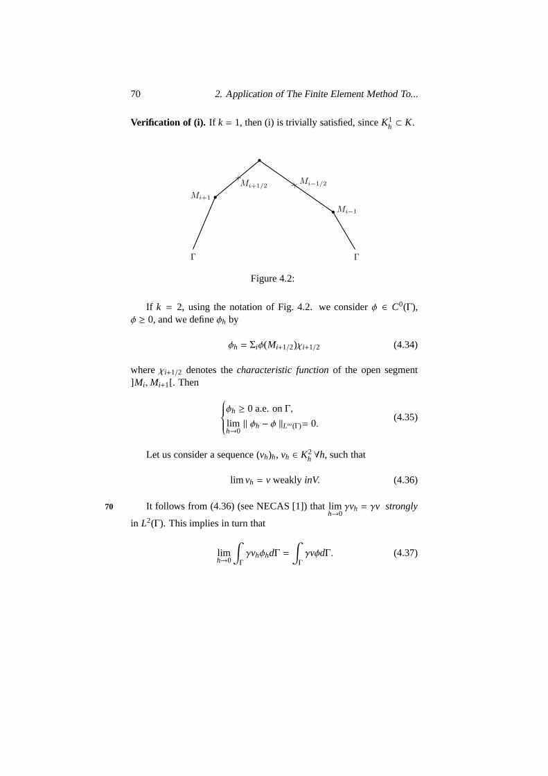
70 2. Application of The Finite Element Method To...
Verification of (i). If k = 1, then (i) is trivially satisfied, sinceK1h ⊂ K.
Figure 4.2:
If k = 2, using the notation of Fig. 4.2. we considerφ ∈ C0(Γ),φ ≥ 0, and we defineφh by
φh = Σiφ(Mi+1/2)χi+1/2 (4.34)
whereχi+1/2 denotes thecharacteristic functionof the open segment]Mi ,Mi+1[. Then
φh ≥ 0 a.e. onΓ,
limh→0‖ φh − φ ‖L∞(Γ)= 0.
(4.35)
Let us consider a sequence (vh)h, vh ∈ K2h ∀h, such that
lim vh = v weakly inV. (4.36)
It follows from (4.36) (see NECAS [1]) that limh→0
γvh = γv strongly70
in L2(Γ). This implies in turn that
limh→0
∫
Γ
γvhφhdΓ =∫
Γ
γvφdΓ. (4.37)

4. A Third Example of EVI of The... 71
It follows from Simpson’s rule that
∫ΓγvhφhdΓ = 1
6Σi |−−−−−−→Mi Mi+1|φ(Mi+1/2)
[vh(Mi) + 4vh(Mi+1/2) + vh(Mi+1)] ≥ 0
∀vh ∈ K2h, ∀φ ∈ C0(Γ), φ ≥ 0.
(4.38)
We obtain from (4.37) and (4.38) that∫
Γ
γvφdΓ ≥ 0∀φ ∈ C0(Γ), φ ≥ 0,
which impliesγv ≥ 0 a.e. onΓ.This proves (i).
Verification of (ii). From Lemma 4.2, it is natural to takeχ = K ∩C∞(Ω). Definerk
h; H1(Ω) ∩C0(Ω)→ Vkh by
rkhv ∈ Vk
h ∀v ∈ H1(Ω) ∩C0(Ω),
rkhv(P) = v(P)∀P ∈ Σk
h, k = 1, 2.(4.39)
On one hand, under the assumptions made onCh we have (seeSTRANG-FIX [1])
‖ rkhv− v ‖V≤ Chk ‖ v ‖Hk+1(ω) ∀v ∈ C∞(Ω), k = 1, 2. (4.40)
with C independent ofh andv.This implies
limh→0‖ rk
hv− v ‖v= 0∀v ∈ χ, k = 1, 2. (4.41)
On the other hand it is obvious thatrkhv ∈ Kk
h ∀v ∈ K ∩ C0(Ω), so thatrkhv ∈ Kk
h ∀v ∈ χ, k = 1, 2.In conclusion, with the aboveχ andrk
h, (ii) is satisfied.
REMARK 4.8. For error estimates in the approximation of(4.5) by 71
piecewise linear finite elements, it has been shown by BREZZI-HAGER-RAVIART [1] that we have
‖ uh − u ‖H1(Ω)= 0(h),
assuming reasonable smoothness hypothesis for u onΩ.

72 2. Application of The Finite Element Method To...
4.6 Iterative methods for solving the discrete problem
We shall briefly describe two types of methods which seem to beappro-priate for solving the approximate problem of Sec. 4.4.
4.6.1 Solution by an over-relaxation method
The approximate problem (Pk1h) are, for k = 1, 2, equivalent to the
quadratic programming problems described in Remark 4.6. Byvirtueof the properties ofKk
h (see Sec. 4.4.1.) we can use, for the solutionof (Pk
1h), the over-relaxation method with projection, which has alreadybeen used in Sec. 2.8 to solve the approximate obstacle problem and isdescribed in CEA [2, Chap. 4]. From the properties of our problem themethod will converge provided 0< ω < 2.
4.6.2 Solution by a duality method
We first consider thecontinuous case.Let us define a LagrangianL by
L (v, q) =12
a(v, v) − L(v) −∫
Γ
qγvdΓ. (4.42)
and letλ be thepositive coneof L2(Γ), i.e.
Λ = q ∈ L2(Γ) : q ≥ 0 a.e. onΓ.
Then we have
THEOREM 4.4. Let L(v) =∫Ω
f vdx+∫Γ
gγvdΓwith f and g sufficientlysmooth. Suppose that the solution u of(4.5)and(4.7)belongs to H2(Ω);thenu, ∂u
∂n − g is the unique saddle point ofL over H1(Ω) × Λ.
Proof. We divide the proof into two parts. In the first part we will show72
thatu, ∂u∂n − g is a saddle point ofL overH1(Ω) × λ and in the second
part we will prove the uniqueness.
(1) Let p = ∂u∂n − g. From the definition of a saddle point we have to
prove thatL (u, q) ≤ L (u, p) ≤ L (v, p)∀v, q ∈ V × Λ,u, p ∈ V × Λ.
(4.43)

4. A Third Example of EVI of The... 73
Sinceu ∈ H2(Ω) we have∂u∂n ∈ H1/2(Γ) ⊂ L2(Γ) (see LIONS -
MAGENES [1]). Then ifg is smooth enough we havep = ∂u∂n − g ∈
L2(Γ). From Proposition 4.1 we have
p = ∂u
∂n − g ≥ 0 onΓ,
p− γu = 0 a.e. onΓ.(4.44)
This implies that we haveu, p ∈ H1(Ω) × Λ and∫Γ
p · γudΓ = 0.Sinceγu ≥ 0 onΓ we have
∫
Γ
q · γudΓ ≥ 0∀q ∈ Λ. (4.45)
It follows from (4.44) and (4.45) that
L (u, q) = 1
2a(u, u) = L(u) −∫Γ
q · γudΓ ≤ 12a(u, u) − L(u) =
= 12a(u, u) − L(u) −
∫Γ
p · γudΓ = L (u, p)∀q ∈ Λ
which proves the first inequality of (4.43).To prove the second inequality of (4.43) we observe that the solution
u∗ of the minimisation problem
L (u∗, p) ≤ L (v, p)∀v ∈ H1(Ω),
u∗ ∈ H1(Ω),(4.46)
is unique and is actually the solution of the linear variational equation 73
a(u∗, v) = L(v) +
∫Γ
pγvdΓ∀v ∈ H1(Ω),
u∗ ∈ H1(Ω).(4.47)
SinceL(v) =∫Ω
f vdx+∫Γ
gγvdΓ, u∗ is actually the solution of the Neu-mann problem
−∆u∗ + u∗ = f in Ω,∂u∗∂n = p+ g = ∂u
∂n onΓ,(4.48)

74 2. Application of The Finite Element Method To...
Since from Proposition 4.1 we obviously have
−∆u+ u = f in Ω,∂u∂n =
∂u∗∂n onΓ,
it follows from the uniqueness property of the Neumann problem (4.48)thatu = u∗. Using (4.46) andu = u∗, we obtain the second inequality in(4.43). This proves thatu, p is a saddle point ofL overH1(Ω) × Λ.
Uniqueness.Let u∗, p∗ be a saddle point ofL over H1(Ω) × Λ.We will show thatu∗ = u, p∗ =. It follows from (4.42) and (4.43) that
∫
Γ
(p− q)γudΓ ≤ 0∀q ∈ Λ. (4.49)
We have similarly,∫
Γ
(p∗, q)γu∗dΓ ≤ 0∀q ∈ Λ. (4.50)
Taking q = p∗ (respectivelyq = p) in (4.49) (respectively (4.50)) weobtain ∫
Γ
(p∗ − p)γ(u∗ − u)dΓ ≤ 0. (4.51)
It follows from the second inequality of (4.43) thatu is the solution of74
a(u, v) = L(v) +
∫Γ
p · γvdΓ∀v ∈ H1(Ω),
u ∈ H1(Ω).(4.52)
ans similarly
a(u∗, v) = L(v) +
∫Γ
p∗ · γvdΓ∀v ∈ H1(Ω),
u∗ ∈ H1(Ω).(4.53)
Taking v = u∗ − u (respectivelyv = u − u∗) in (4.52) (respectively(4.53)) we obtain
a(u∗ − u, u∗ − u) =∫
Γ
(p∗ − p)γ(u∗ − u)dΓ. (4.54)

4. A Third Example of EVI of The... 75
Using theV-ellipticity of a(·, ·) it follows then from (4.51)–(4.54) thatu∗ = u and ∫
Γ
(p∗ − p)γvdΓ = 0∀v ∈ H1(Ω),
which implies thatp∗ = p.Henceu, p is the unique saddle point ofL overH1(Ω) × Λ.It follows from Theorem 4.4 that we can apply Uzawa’s algorithm
to solve (4.5) (see CEA [2, Chap. 5], G.L.T. [1, Chap.2], [2, Chap. 4,Sec 3.6]). In the present case this algorithm is written as follows:
p0 ∈ Λ is arbitrarily chosen (for instancep0 = 0). (4.55)
By induction, after knowing pn we computeun, pn+1 by
L (un, pn) ≤ L (v, pn)∀v ∈ H1(Ω), un ∈ H1(Ω), (4.56)
pn+1 = PΛ(pn − ργun), (4.57)
wherePΛ is projection operatorfrom L2(Γ) to Λ in the L2(Γ) norm 75
andρ > 0. It follows from (4.56) thatun is in fact the solution of theNeumann problem
−∆un + un = f in Ω,∂un
∂n |Γ = pn + g.(4.58)
The projectionPΛ is given by
PΛ(q) = q+ ∀q ∈ L2(Γ). (4.59)
Sinceγ : H1(Ω)→ L2(Γ) is a continuous linear map we have
‖ γv ‖L2(Γ)≤‖ γ ‖ · ‖ v ‖H1(Ω) ∀v ∈ H1(Ω). (4.60)
It follows then from CEA, G.L.T., loc. cit., that
limn→∞
un = u strongly inH1(Ω), (4.61)
whereu is the solution of the problem (4.5) provided that 0< ρ < 2‖γ‖2 .

76 2. Application of The Finite Element Method To...
Let us give a direct proof for this convergence result. This proofwill use the characterisation (4.5) given in Proposition 4.1 (even ifa(·, ·)is not symmetric the same result follows). It will be convenient to take(4.56), (4.58) in the following equivalent form:
a(un, v) = L(v) +
∫Γ
pnγvdΓ∀v ∈ H1(Ω),
un ∈ H1(Ω).(4.62)
Let u be the solution of (4.5) andp = ∂u∂n − g. It follows from
Proposition 4.1 that
a(u, v) = L(v) +∫Γ
pγvdΓ∀L ∈ H1(Ω),
u ∈ H1(Ω),(4.63)
∫
Γ
(q− p)γudΓ ≥ 0∀q ∈ Λ, p ∈ Λ. (4.64)
Relation (4.64) can also be written as76∫
Γ
(q− p)(p− ργu− p)dΓ ≤ 0∀q ∈ Λ, ρ > 0.
which is classically equivalent to
p = PΛ(p− ργu). (4.65)
Let consider:un= un − u, pn
= pn − p.
SincePΛ is a contraction , we have from (4.57) and (4.65)
‖ pn+1 ‖L2(Γ)≤‖ pn − ργun ‖L2(Γ) . (4.66)
It follows from (4.66) that
‖ pn ‖2L2(Γ)‖ pn+1 ‖L2(Γ)≥ 2ρ∫
Γ
γunpndΓ − ρ2 ‖ γun ‖2L2(Γ) . (4.67)
Takingv = un (4.62) and (4.63) we obtain
a(un, un) =∫
Γ
pnγundΓ. (4.68)

4. A Third Example of EVI of The... 77
It follows then from (4.67) and (4.68) that
‖ pn ‖2L2(Γ) − ‖ pn+1 ‖2L2(Γ)≥ ρ(2− ρ ‖ γ ‖2) ‖ un ‖2H1(Ω) . (4.69)
If 0 < ρ < 2‖γ‖2 we observe that the sequence‖ pn ‖2
L2(Γ)n is decreasing
and hence converges. Therefore we have
limn→∞
(‖ pn ‖2L2(Γ) − ‖ pn+1 ‖2L2(Γ)) = 0
so thatlimn→∞‖ un ‖H1(Ω)= 0.
Sinceun= un − u, we have proved the convergence. 77
Similarly we can solve the approximate problem (Pk1h), k = 1, 2,
using the discrete version of algorithm (4.55)–(4.57). We shall limitourselves tok = 1, since the extension here tok = 2 is almost trivial.
We use here the notations of Sec. 4.1. Assume thatγh = Σh−Σ0h has
been ordered.Let γh = Mii .We approximateΛ andL by
Λ1h = qh : qh = qii , qi ≥ 0 and
L 1
h (vh, qh) = 12a(vh, vh) − L(vh)
−12Σi |Mi Mi+1|[qivh(Mi) + qi+1vh(Mi+1)].
(2.2)
We can prove thatL 1h has a unique saddle pointuh, ph whereph is
a F. John-Kuhn-Tucker vector for (P11h) overV1
h ×Λ1h anduh is precisely
the solution of (P11h). The discrete analogue of (4.55)–(4.57) is then
p0h ∈ Λ
1h. (4.71)
L 1
h (unh, p
nh) ≤ L 1
h (vh, pnh)∀vh ∈ V1
h ,
unh ∈ V1
h .(4.72)
pn+1i = [pn
i − ρunh(Mi)]
+ ∀i, ρ > 0. (4.73)

78 2. Application of The Finite Element Method To...
One can prove that if 0< ρ < β, β small enough, then limn→+∞
unh = uh
whereuh is the solution of (P11h). One may find in G.L.T. [2, Chap.4] nu-
merical applications of the above iterative methods for piecewise linearand piecewise quadratic approximations of (4.5).
Exercise 4.3.Extend the above considerations to(P21h).
5 An Example of EVI of The Second Kind: A Sim-plified Friction Problem
5.1 The continuous problem. Existence and Uniqueness re-sults
78
Let Ω be a bounded domain ofR2 with a smooth boundaryΓ = ∂Ω.Using the same notations as in Sec. 4 we define
V = h1(Ω), (5.1)
a(u, v) =∫
Ω
∇u · ∇vdx+∫
Ω
uvdx. (5.2)
L(v) =< f , v >, f ∈ V∗, (5.3)
j(v) = g∫
Γ
|γv|dΓ, whereg > 0. (5.4)
We have then the following
THEOREM 5.1. The variational inequality
a(u, v− u) + j(v) − j(u) ≥ L(v− u)∀v ∈ V.
u ∈ V.(5.5)
has a unique solution.
Proof. In order to apply Theorem 4.1 of Chap. 1, it is enough to verifythat j(·) is convex, proper and l.s.c. Actuallyj(·) is a seminorm on

5. An Example of EVI of The Second Kind:... 79
V. Therefore using Schwartz inequality inL2(Γ) and the fact thatγ ∈L (H1(Ω), L2(Γ)) we have
| j(u) − j(v)| ≤ | j(u− v)| ≤ g(meas· Γ)1/2 ‖ γ(v− u) ‖L2(Γ)≤ C ‖ u− v ‖V,(5.6)
for some constantC.
Hence j(·) is Lipschitz continuous onV, so thatJ(·) is l.s.c ; j(·) isobviously convex and proper. Hence the Theorem is proved.
REMARK 5.1. If g = 0, it is easy to prove that(5.5) reduce to thevariational equation
a(u, v) = L(v)∀v ∈ V,
u ∈ V.
This is related to the variational formulation of the Neumann problem.
REMARK 5.2. Since a(·, ·) is symmetric,. the solution u of a(5.5) is 79
characterised, using Lemma 4.1 of Chap. 1, as the unique solution ofthe minimization problem
J(u) ≤ J(v), ∀v ∈ V,
u ∈ V,(5.7)
where J(v) =12
a(v, v) + j(v) − L(v).
REMARK 5.3. The problem(5.5) (and (5.7)) is the simplified versionof a friction problem occurring inelasticity. For this types of problemswe refer to DUVAUTLIONS [1]and the bibliography therein.
Exercise 5.1.Let us denote by ug the solution of(5.5). Then prove that
limg→+∞
ug = U strongly in H1(Ω),
whereu is the unique solution ofa(u, v) = L(v)∀v ∈ H1
0(ω),
u ∈ H10(Ω).

80 2. Application of The Finite Element Method To...
5.2 Regularity of the solution
THEOREM 5.2. (H. BREZIS [3]). IfΩ is a bounded domain witha smooth boundary and if L(v) =
∫Ω
f vdx with f ∈ L2(Ω), then thesolution u of(5.5) is in H2(Ω).
5.3 Existence of a multiplier
Let us defineΛ by
Λ = µ ∈ L2(Γ) : |µ(x)| ≤ 1 a. e. inΓ.
Then we have
THEOREM 5.3. The solution u of(5.5) is characterised by the exis-tence ofλ such that
a(u, v) + g
∫ΓλγvdΓ = L(v)∀v ∈ V,
u ∈ V,(5.8)
λ ∈ Λ,λγu = |γu| a. e. inΓ.
(5.9)
80
Proof. We will prove first that (5.5) implies (5.8) and (5.9).Takingv = 0 andv = 2u in (5.5) we have
a(u, u) + j(u) = L(u). (5.10)
It follows then from (5.5), (5.10) that
L(v) − a(u, v) ≤ j(v)∀v ∈ V,
which implies
|L(v) − a(u, v)| ≤ j(v) = g∫
Γ
|γv|dΓ∀v ∈ V. (5.11)

5. An Example of EVI of The Second Kind:... 81
We haveH1(Ω) = H10(Ω)⊕ [H1
0(Ω)]⊥ where [H10(Ω)]⊥ is the orthog-
onal complement ofH10(Ω)in H1(Ω).
Sinceγ : [H10(Ω)]⊥ → H1/2(Γ) is an isomorphism, it follows from
(5.11) thatL(v) − a(u, v) = ℓ(γv)∀v ∈ V, (5.12)
whereℓ(·) is a continuous linear functional onH1/2(Γ). It follows thenfrom (5.11), (5.12) that
|ℓ(µ)| ≤ g ‖ µ ‖L1(Γ) ∀µ ∈ H1/2(Γ). (5.13)
SinceH1/2(Γ) ⊂ L1(Γ) it follows from (5.13) that, we can apply toℓ(·), the Hanh-Banach Theorem (see for instance YOSIDA [1]) to obtainthe existence ofλ ∈ L∞(Γ), |λ(x)| ≤ 1 a.e. inΓ such that
ℓ(µ) = g∫
Γ
λµdΓ∀µ ∈ H1/2(Γ). (5.14)
Therefore it follows from (5.12) and (5.14) that 81
a(u, v) + g∫
Γ
λγvdΓ = L(v)∀v ∈ V,
which proves (5.8).Takingv = u in (5.8) we obtain
a(u, u) + g∫
Γ
λγudΓ = L(u).
Using (5.10) and the above equation we obtain∫
Γ
(|γu| − λγu)dΓ = 0. (5.15)
Since|λ| ≤ 1 a.e. we have
|γu| − λγu ≥ 0 a.e. (5.16)
It follows from (5.15) and (5.16) that
|γu| = λγu a.e.

82 2. Application of The Finite Element Method To...
This completes the proof of (5.8) and (5.9). Assuming (5.8) and (5.9)we will show that (5.5) holds.
Let u, λ be a solution of (5.8), (5.9). It follows from (5.8) that
a(u, v− u) + g∫
Γ
λγ(v− u)dΓ = L(v− u)∀v ∈ V,
which can also be written as
a(u, v− u) + g∫
Γ
λγvdΓ − g∫
Γ
λγudΓ = L(v− u)∀v ∈ V. (5.17)
From (5.9) and (5.17) we obtain
a(u, v− u) + g∫
Γ
λγvdΓ − g∫
Γ
|γu|dΓ = L(v− u)∀v ∈ V. (5.18)
But sinceλγv ≤ |γv| a.e. inΓ, it follows from (5.18) that
a(u, v− u) + j(v) − j(u) ≥ L(v− u)∀v ∈ V.
This proves the characterization.82
REMARK 5.4. Assuming that
L(v) =∫
Ω
f0vdx+∫
Γ
f1γvdΓ,
with f0, f1 sufficiently smooth, we can express(5.8)by−∆u+ u = f0 in Ω,∂u∂n + gλ = f1 a. e. onΓ.
(5.19)
It follows from(5.19)thatλ is unique.
Exercise 5.2.Prove thatλ is unique∀L ∈ V∗.
5.4 Finite element approximation of (5.5)
LetΩ be a bounded domain ofR2. The notation used here is mostly thesame as in Sec. 4.4 of this Chapter.

5. An Example of EVI of The Second Kind:... 83
5.4.1 Approximation of V
We use the piecewise linear and piecewise quadratic approximations ofV = H1(Ω) described in Section 4.4.1 of this chapter.
5.4.2 Approximation of j(·)
We use the notation of Figure 4.2. Then we approximatej(·) by
j1h(vh) =g2
∑
i
|−−−→Mi Mi+1|(|γvh(Mi)| + |γvh)Mi+1)|)∀vh ∈ V1h , (5.20)
j2h(vh) =
g6
∑i |−−−→Mi Mi+1|(|γvh(Mi)| + 4|γvh(Mi+1/2|
+|γvh(Mi+1)|)∀vh ∈ V2h .
(5.21)
In (5.20) and (5.21) we haveMi ∈ γh andMi+1/2 ∈ γ′h.
REMARK 5.5. Clearly (5.20), (5.21) are respectively obtained fromj(·) by using Trapezoidal and Simpson’s numerical integration formu-lae.
5.4.3 The approximate problem
Fork = 1, 2 the problem (5.5) is approximated by 83
(Pk2h)
a(uk
n, vh − ukh) + jkh(vh) − jkh(uk
h) ≥ L(vh − ukh)∀vh ∈ Vh,
ukh ∈ Vk
h.
Then,
Proposition 5.1. The problem(Pk2h) has a unique solution.
REMARK 5.6. Since a(·, ·) is symmetric,(Pk2h) is equivalent to the non-
linear programing problem
minvh∈Vk
h
[12
a(vh, vh) + jkh(vh) − L(vh)
]. (5.22)
REMARK 5.7. Using(5.20), (5.21)and (7.1)–(7.4)of Section 7 of thischapter, we may express(Pk
2h) and (5.22) in a form more suitable forcomputations.

84 2. Application of The Finite Element Method To...
5.5 Convergence results
THEOREM 5.4. Suppose that the angles ofCh are uniformly boundedbelow byθ > 0 as h→ 0, then
limh→0
ukh = u strongly in H1(Ω), (5.23)
where u and ukh are respectively the solutions of(5.5) and (Pk2h) for k =
1, 2.
Proof. To prove (5.23) it is enough to verify the following (see Theo-rem 6.3 of Chapter 1)
(i) There existsU ⊂ V, U = V and
rkh : U → Vk
h such that
limh→0
rkhv = v strongly inV ∀v ∈ U,
(ii) If Vh→ v weakly in V then
lim infh→0
jkh(vh) ≥ j(v).
(iii) limh→0
jkh(rkhv) = j(v)∀v ∈ U.84
Verification of (i). SinceΓ is Lipschitz continuous we have (see NECAS[1])
C∞(Ω) = H1(Ω). (5.24)
Therefore it is natural to takeU = C∞(Ω). Define rkh by (4.39)
if Theorem 4.3, chap. 2; under the above assumption onCh it followsfrom STRANG-FIX [1] that
‖ rkhv− v ‖V≤ Chk ‖ v ‖Hk+1(Ω) ∀v ∈ V, (5.25)
whereC is a constant independent ofh andv. This implies (i).
Verification of (ii).

5. An Example of EVI of The Second Kind:... 85
(1) Case k= 1. We use again the notation of Figure 4. 2. Since thetrace ofvh restricted to [Mi ,Mi+1] is affine it follows that
yvh(M) = 1
|Mi Mi+1| (|−−−→MMi+1|γvh(Mi) + |
−−−→MMi |γvh(Mi+1)),
∀vh ∈ V1h , ∀M ∈ [Mi ,Mi+1].
(5.26)
Since|−−−→MMi+1|
|−−−→Mi Mi+1|+|−−−→MMi |
|−−−→Mi Mi+1|= 1,
the convexity ofξ → |ξ| implies|γvh(M)| ≤ 1
|−−−−→Mi M i+1|(|−−−→MMi+1||γvh(Mi)|
+|−−−→Mi M| |γvh(Mi+1)|)∀vh ∈ V1h , ∀M ∈ [Mi ,Mi+1].
(5.27)
Interesting (5.27) onMi Mi+1 we obtain
∫
Mi Mi+1
|γvh|dΓ ≤|−−−→Mi Mi+1|
2(|γvh(Mi)| + |γvh(Mi+1)|)
which implies that∀vh ∈ V1h we have
j(vh) = g∫Γ|γvh|dΓ = g
∑i
∫Mi Mi+1|γvh|dΓ ≤
≤ g2
∑i|−−−→Mi Mi+1|(|γvh(Mi)| + |γvh(Mi+1)|)
= j1h(vh).
Thus we have proved 85
j(vh) ≤ j1h(vh)∀vh ∈ V1h . (5.28)
Let vh → v weaklyin V. Then limh→0
γ(vh) = γ(v) strongly in L2(Γ),
which implieslimh→0
j(vh) = j(v). (5.29)
It follows then from (5.28) and (5.29) that limh→0
inf j1h(vh) ≥ j(v), which
proves (ii) ifk = 1.

86 2. Application of The Finite Element Method To...
(2) case k= 2. Let us defineMi+1/6′Mi+5/6 by (see Figure 5.1)
−−−→Mi Mi+1/6 =
16−−−→Mi Mi+1,
−−−→Mi Mi+5/6 =
56−−−→Mi Mi+1.
Figure 5.1:
Then we defineqh : C0(Γ) + L∞(Γ) by86
qh(µ) =∑
Mi∈γh
µ(mi)Xi +∑
M i+12∈γ′h, µ(Mi+1/2)Xi+1/2
∀µ ∈ C0(Γ).(5.30)
where Xi ( respectively Xi+1/2) is the characteristic function ofMi−6Mi Mi+1/6 (respectively Mi+1/6Mi+5/6). We have then the follow-ing obvious properties :
limh→0
qh(µ) = µ strongly inL∞(Γ) ∀µ ∈ C(Γ), (5.31)
j2h(vh) = g∫
Γ
|qhγvh|dΓ = g ‖ qhγvh ‖L1(Γ) ∀vh ∈ V2h , (5.32)
C1 ‖ γvh ‖L2(Γ)≤‖ qhγvh ‖L2(Γ)≤ C2 ‖ γvh ‖L2(Γ) ∀vh ∈ V2h , (5.33)
where in (5.33),C1 andC2 are positive constants independent ofvh, handΓ (values forC1 andC2 may be found in G. L. T. [2, Chap. 4]).

5. An Example of EVI of The Second Kind:... 87
Now takingµ ∈ C0(Γ), we definesh(µ) by
sh(µ) ∈ L∞(Ω),
sh(µ)|]Mi ,Mi+1[ = µ(Mi+1/2).(5.34)
Thenlimh→0
sh(µ) = µ strongly inL∞(γ), (5.35)
and from Simpson’s integration formula we have∫
Γ
sh(µ)qhγhvhdΓ =∫
Γ
sh(µ)γvhdΓ ∀µ ∈ C(Γ),∀vh ∈ V2h . (5.36)
Let vh→ v weakly inV, vh ∈ V2h ∀h, then
limh→0
γvh = γv strongly inL2(Γ). (5.37)
On the one hand it follows from (5.33) that 87
‖ qhγvh ‖L2(Γ)≤ C, (5.38)
whereC is independent ofh.On the other hand (5.31), (5.35)–(5.38) imply that
limh→0
∫
Γ
sh(µ)qhγvhdΓ =∫
Γ
µγvdΓ ∀µ ∈ C0(Γ). (5.39)
In turn (5.38) and (5.39) imply that
limh→0
qhγvh = v weakly inL2(Γ). (5.40)
Since the functionalµ →‖ µ ‖L1(Γ) is convex and continuous onL1(Γ) it follows from (5.40) that
lim infh→0
‖ qhγvh ‖L1(Γ)≥‖ γv ‖L1(Γ) (5.41)
Combining (5.41) with (5.32) we obtain lim infh→0
j2h(vh) ≥ j(v) which
proves (ii) whenk = 2.

88 2. Application of The Finite Element Method To...
Verification of (iii). Let v ∈ U = C∞(Ω). From (5.25) and from theuniform continuity ofγv onΓ it follows almost immediately that
limh→0
jkh(rkhvh) = j(v), k = 1, 2.
Since the condition (i), (ii) and (iii) are satisfied the strong conver-gence ofuh to u follows from the Theorem 6.2 of Chap. 1.
REMARK 5.8. It is proved in G. L. T. [2, Chap. 4] that vh→ v weaklyin v, v/2 ∈ Vk
h, implieslimh→0
jkh(vh) = j(v), k = 1, 2.
Since the proof of this result is rather technical we have used in thesenotes a simpler approach from which it follows that
lim infh→0
jkh(vh) ≥ j(v), k = 1, 2.
As we have seen before this result was sufficient for proving Theo-rem 5.4.
5.6 Iterative methods for solving(Pk2h).
In this section we briefly describe some iterative methods which may be88
useful for solving the approximate problems (Pk2h).
5.6.1 Solution of(Pk2h) by relaxation methods
It follows from (5.20)–(5.22) (see Remark 5.6) that (Pk2h), k = 1, 2, are
particular cases ofminv∈RN
f (v), (5.42)
where, withv = (v1, . . . , vn),
f (v) =12
(Av, v) − (b, v) +N∑
i=1
αi |vi |. (5.43)
In (5.43), (·, ·) denotes the usual inner product ofRN, A is aN × Nsymmetric positive definite matrix andαi ≥ 0 ∀i = 1, . . . ,N.

5. An Example of EVI of The Second Kind:... 89
It follows then from CEA [2, Chap. 4], CEA-GLOWINSKI [1], G.L. T. [1, Chap, 2] that we can use a relaxation method for solving (5.42).Actually from the computation parameterω, ω > 1, will increase thespeed of convergence.
Finally the algorithm we used is the following :
u0 arbitrarily given inRN, (5.44)
then fori = 1, 2, . . . ,N,
f (un+11 , . . . , un+1
i−1 , u−n+1i , un
i+1, . . .) ≤f (un+1
1 , . . . , un+1i−1 , vi , u
n+1i+1 , . . .)∀vi ∈ R, (5.45)
un+1i = un
i + ω(un+1i − un
i ). (5.46)
If ω = 1, (5.44)–(5.46) reduces to a relaxation method. Numericalsolu-tions of (5.5) using (5.44)–(5.46) are given in G. L. T. [2, Chap. 4].
REMARK 5.9. If αi > 0, u−n+1i is the solution of aone variable, non
differentiable minimization problemwhich can be exactly computed byhand calculation.
Exercise 5.3.Express u−n+1i as a function of A, b, un, un+1.
5.6.2 Solution of(Pk2h by duality method)
We first examine the continuous case. Define a LagrangienL : H1(Ω)× 89
L2(Γ)→ R by
L (v, µ) =12
a(v, v) − L(v) + g∫
Γ
µγvdΓ. (5.47)
Then using the notation of Sec. 5.3 it follows from Theorem 5.3 that
THEOREM 5.5. Let u, λ be a solution of(5.8), (5.9) ; then u, λ isthe unique saddle point ofL over H1(Ω) × Λ
Exercise 5.4.Prove Theorem 5.5.

90 2. Application of The Finite Element Method To...
From Theorem 5.5 it follows that to solve(5.5) we can use the fol-lowing Uzawa’s algorithm,
λ0 ∈ Λ arbitrarily chosen (for instanceλ0 = 0), (5.48)
then by induction, knowingλn we compute un andλn+1 byL (un, λn) ≤ L (v, λn)∀v ∈ H1(Ω),
un ∈ V,(5.49)
λn+1 = PΛ(λn + ρgγun), ρ > 0. (5.50)
The minimization problem (5.49) is actually equivalent to theNeu-mann variational problem
a(un, v) = L(v) − g
∫ΓλnγvdΓ∀v ∈ H1(Ω),
un ∈ H1(Ω).(5.51)
In (5.50).PΛ is the projection operator fromL2(Γ) toΛ in theL2− norm,then
PΛ(µ) = sup(−1, inf(1, µ)) ∀µ ∈ L2(Γ). (5.52)
Using CEA [2], G. L. T. [1, Chap. 2] it follows that for 0< ρ < 2g2‖γ‖2 .
we have limn→∞
un = u strongly inH1(Ω),
u solution of (5.5), (5.7).90
Like in Section 4.6.2 a direct proof of the convergence of (5.48)–(5.50) can be given : it will however use the results of Theorem 5.3.
Exercise 5.5.Using Theorem 5.3, given a direct proof of the conver-gence of(5.48)–(5.50).
The adaptation of(5.48)–(5.50) to the discrete problem(Pk2h), k =
1, 2, is straightforward (see G. L.T. [2, Chap, 4]), since it is a simplevariant of the discrete algorithm described in section 4.6.2.
Exercise 5.6.Study the discrete analogues of(5.48)–(5.50) related to(Pk
2h), k = 1, 2.

6. A Second Example of EVI of The... 91
6 A Second Example of EVI of The Second Kind:The Flow of A Viscous, Plastic Fluid in A Pipe
Most of the material in this section can be found in G.L.T. [1,Chap. 5]and in GLOWINSKI [1], [3].
6.1 The continuous problem. Existence and uniqueness re-sults
LetΩ be a bounded domain ofR2 with a smooth boundaryΓ. We define
V = H10(Ω).
a(u, v) =∫Ω∇u · ∇vdx,
L(v) =< f , v >, f ∈ V∗
j(v) =∫Ω|∇v|dx
Let µ, g be two positive parameters ; then
THEOREM 6.1. The variational inequality
µa(u, v− u) + g j(v) − g j(u) ≥ L(v− u) ∀v ∈ V,
u ∈ V(6.1)
has a unique solution. 91
Proof. In order to apply Theorem 4.1 of Chap. 1, we only have to verifythat j(·) is convex, proper and l.s.c.
It is obvious thatj(·) is convex and proper, Letu, v ∈ V; then
| j(v) − j(u)| ≥√
meas.Ω ‖ u− v ‖V, (6.2)
hencej(·) is l.s.c.This proves the Theorem.
Exercise 6.1.Prove that j(·) is a norm on V.

92 2. Application of The Finite Element Method To...
REMARK 6.1. If we take g= 0 in (6.1) we recover the variationalformulation of the Dirichlet problem
−µ∆u = f in Ω,
u = 0 onΓ.
REMARK 6.2. Since a(·, ·) is symmetric, the solution u of(6.1)is char-acterized, using Lemma 4.1 of Chap. 1, as the unique solutionof theminimization problem
J(u) ≤ J(v) ∀v ∈ V,
u ∈ V,(6.3)
where J(v) = µ2a(v, v) + g j(v) − L(v).
6.2 Physical motivation
If L(v) = C∫Ω
vdx(for instanceC > 0), it is proved in DUVAUT-LIANS[1, Chap. 6] that (6.1) models thelaminar, stationary flowof aBinghamfluid in a cylindrical pipe of cross - sectionΩ, u(x) being the velocityat x ∈ Ω (We refer to PRAGER [1], GERMAIN [1] and DUVAUT -LIONS [1, Chap. 6] for the definition of Bingham fluid). The constantC is the linear decay of pressureandµ, g are respectively theviscosityand plasticity yield of the fluid. The above medium behaves like aviscous fluid (of viscosityµ) in Ω+ = x ∈ Ω : |∇u(x)| > 0 and like arigid medium inΩ0 = x ∈ Ω : ∇u(x) = 0. We refer to MOSSOLOV-92
MIASNIKOV [1], [2], [3] for a detailed study of the properties ofΩ+
andΩ0. We observe that (6.1) appears also as afree boundary problem.
6.3 Regularity properties
THEOREM 6.2. (H. BREZIS [4]). If L(v) =∫Ω
f vdx, f ∈ L2(Ω) thenthe solution u of(6.1)satisfies
u ∈ V ∩ H2(Ω)
and ifΩ is convex, we have
‖ u ‖H2(Ω)≤γ(Ω)µ‖ f ‖L2(Ω) (6.4)

6. A Second Example of EVI of The... 93
6.4 Further properties
Let us denote byα the following quantity
α = infv∈H1
0(Ω)v,0
j(v)‖ v ‖L1(Ω)
(6.5)
Thenα > 0.
We derive from this the following
Proposition 6.1. Let u be the solution of (6.1) and f∈ L∞(Ω), thenu = 0 if
‖ f ‖L∞(Ω)≤ gα. (6.6)
Proof. By takingv = 0, v = 2u in (6.1) we obtain
µa(u, u) + g(u) =∫
Ω
f udx. (6.7)
It follows then from (6.5) and from∫Ω
f udx ≤‖ f ‖L∞(Ω)‖ u ‖L1(Ω),that
µa(u, u) + (gα− ‖ f ‖L∞(Ω)) ‖ u ‖L1(Ω)≤ 0. (6.8)
If f obeys (6.6) it follows then from (6.8) thatu = 0. We also have
Proposition 6.2. Let u be the solution of(6.1) and f ∈ Lp(Ω), p > 1. 93
Then if f ≥ 0, we have u≥ 0.
Exercise 6.2.Prove Proposition 6.2.
Proposition 6.3. Let u be the solution of(6.2) and f = c, a constant.Then u= 0 ⇐⇒ c ≤ g and u, 0 if c > gα.
Exercise 6.3.Prove Proposition 6.3

94 2. Application of The Finite Element Method To...
Proposition 6.4. Let u be the solution of(6.1) and f ∈ L2(ω); thenu = 0 if
‖ f ‖L2(ω)≤ gβ, (6.9)
where
β = infv∈H1
0(Ω)v,0
j(v)‖ v ‖L2(Ω)
.
Proof. It follows from a result of L. NIRENBERG and M. STRAUSS(cf. STRAUSS [1]) thatβ > 0.
By takingv = 0 andv = u in (6.1) we obtain
µa(u, u) + g j(u) =∫
Ω
f udx. (6.10)
Using∫Ω
f udx≤‖ f ‖L2(Ω)‖ u ‖L2(Ω) andβ > 0 we obtain
µa(u, u) + (gβ− ‖ f ‖L2(Ω)) ‖ u ‖L2(Ω)≤ 0. (6.11)
Hence if f satisfies (6.9) we have from (6.11) thata(u, u) = 0. Thisimpliesu = 0, hence the Proposition.
6.5 Exact solutions
6.5.1
Example 1. We takeω =]0, 1[ and f = c, c a positive constant. In thiscase the solution of
µ∫ 10 u(v′ − u′)dx+ g
∫ 10 |v
′|dx− g∫ 10 |u
′|dx≥c∫ 10 (v− u)dx ∀v,H1
0(Ω),
u ∈ H10(Ω),
(6.12)
(where v′ =dvdx
) is given by94
u = 0 if g ≥c2. (6.13)

6. A Second Example of EVI of The... 95
If g ≤c2
then
u(x) = c2µ x(1− x) − gx
µ if 0 ≤ x ≤ 12 −
gc
u(x) = c2µ (1
2 −gc)2 if 1
2 −gc ≤ x ≤ 1
2 +gc ,
u(x) = ceµ x(1− x) − g
µ (1− x) if 12 +
gc ≤ x ≤ 1.
(6.14)
We observe that ifg < c2 thenu ∈ H1
0(Ω)∩W2,∞(ω), butu < H3(Ω).
6.5.2
Example 2. Letω = x : x21 + x2
2 < R2, f = C, C a positive constant.Then the solution of(6.1) is given by
u = 0 if g ≥ CR2, (6.15)
If g ≤ CR2 then
u(x) = (R−r2µ )[ C
2 (R+ r) − 2g] if R′ ≤ r ≤ R,
u(x) = (R−R′2µ )[ C
2 (R+ R′) − 2g] if 0 ≤ r ≤ R,
(6.16)
where
r =√
x21 + x2
2,R′ =
2gC
We observe also that ifg < CR2 then u ∈ H1
0(Ω) ∩ W2,∞(Ω) butu < H3(Ω) (we have actuallyu ∈ Hs(Ω), s< 5
2).
Exercise 6.4.Verify that(6.13), (6.14)and (6.15), (6.16)are solutionsof (6.12)and (6.1) respectively.
6.6 Existence of multipliers
Let us defineΛ by
Λ = q : q ∈ L2(Ω) × L2(Ω), |q(x)| ≤ 1 a.e.
|q(x)| =√
q21(x) + q2
2(x); then we have
95

96 2. Application of The Finite Element Method To...
THEOREM 6.3. The solution u of(6.1) is characterised by the exis-tence of p such that
µa(u, v) + g
∫Ω
p.∇vdx=< f , v > ∀v ∈ V,
u ∈ V,(6.17)
p.∇u = |∇u|a.e.,p ∈ Λ.
(6.18)
Proof. There are classical proofs of the above Theorem using Min-Maxof Hahn-Banach Theorems (see for instance CEA [2, Chap. 5], G. L. T/[1 , Chap. 1], EKELAND- TEMAM [1]). In the sequel following G.L.T. [2 , Chap. 5] we shall give an “almost constructive ” proof makinguse of a regularisation technique.
(1) We first prove that(6.17), (6.18)imply (6.1). It follows from (6.17)that
µa(u, v− u) + g∫Ω
p · ∇(v− u)dx= µa(v− u)
+g∫Ω
p · ∇vdx− g∫Ω
p · ∇udx=
=< f , v− u > ∀v ∈ V.
(6.19)
It follows from (6.18) that∫
Ω
p.∇udx=∫
Ω
|∇u|dx, (6.20)
and from the definition ofΛ that∫
Ω
p.∇vdx≤∫
Ω
|p| · |∇v|dx ≤∫
Ω
|∇v|dx ∀v ∈ V. (6.21)
Then from (6.17), (6.19)–(6.21) we obtain that
µa(u, v− u) + g j(u) ≥< f , v− u > ∀v ∈ V,
u ∈ V.

6. A Second Example of EVI of The... 97
Thus (6.17) and (6.18) implies (6.1).
(2) Necessity of(6.17)and (6.18). Takingu = 0 andv = 2u in (6.1) we96
obtainµa(u, u) + g j(u) =< f , u > . (6.22)
Let ∈> 0. Regularisej(·) by jǫ(·) defined byjǫ(v) =∫Ω
√∈2 +v2dx.
Since jǫ(·) is convex and continuous onV, the regularised problemµa(uǫ , v− uǫ ) + g jǫ (uǫ ) ≥ L(v− uǫ )∀v ∈ V,
uǫV,(6.23)
has auniquesolution. Let us show that lim∈→0
uǫ = u strongly in V.
From (6.1) and (6.23) it follows that
µa(uǫ , u− uǫ ) + g jǫ (u) − g jǫ(uǫ ) ≥ L(u− uǫ),
µa(u, uǫ − u) + g j(uǫ ) − g j(u) ≥ L(uǫ − u).
Adding these inequalities we obtain
µa(uǫ − u, uǫ − u) + g( jǫ (uǫ) − j(uǫ )) ≤ g( jǫ (u) − j(u)). (6.24)
From 0<√
t2+ ∈2− |t| = ∈2√∈2+t2+|t|
≤∈ ∀t ∈ R it follows thatµa(uǫ , uǫ −u) ≤ g ∈ meas. (Ω), so that
‖ uǫ − u ‖V≤√
meas.(Ω)(gu. ∈)1/2 (6.25)
From (6.25) we obtain
lim∈→0
uǫ = u strongly inV. (6.26)
Since jǫ(·) is differentiable onV, the problem (6.23) is equivalent (seeCEA [1]) to the following non-linear variational equation:
µa(uǫ , v) + g < j′ǫ(u), v >= L(v)∀v ∈ V,
uǫ ∈ V,(6.27)
with 97
98 2. Application of The Finite Element Method To...
< j′ǫ(w), v >=∫
Ω
∇w · ∇v√∈2 +|∇w|2
dx∀v,w ∈ V. (6.28)
If we define (pǫ ) by
Pǫ =∇uǫ√∈2 +|∇uǫ |2
(6.29)
thenpǫ ∈ Λ. (6.30)
From (6.27)–(6.30) we obtainµa(uǫ , v) + g
∫Ω
pǫ · ∇vdx= L(v) ∀v ∈ V,
uǫ ∈ V.(6.31)
SinceΛ is a bounded, closed, convex subset ofL2(Ω) × L2(Ω) it isweakly compact, so that from (pǫ)ǫ we can extract a subsequence, stilldenoted by (pǫ )ǫ such that
lim∈→0 pǫ = p weakly inL2(Ω) × L2(Ω),
p ∈ Λ.(6.32)
Actually we havepǫ → p in L∞(Ω) × L∞(Ω) weakly *.Taking the limit as∈→ 0 in (6.31) we have from (6.26) and (6.32)
µa(u, v) + g
∫Ω
p · ∇vdx= L(v) ∀v ∈ V,
u ∈ V,(6.33)
so that (6.17) is proved.To complete the proof of the Theorem we have only to prove that98
p · ∇u = |∇u| a.e. (6.34)
Takingv = u in (6.33) and comparing with (6.22) we obtain∫
Ω
|∇u|dx−∫
Ω
p · ∇udx=∫
Ω
(|∇u| − p · ∇u)dx= 0. (6.35)
Sincep ∈ Λ, it follows from Schwartz inequality inR2 that
p · ∇u ≤ |∇u|a.e.

6. A Second Example of EVI of The... 99
Combining (6.35) and this inequality we obtain
p · ∇u = |∇u|a.e.
This proves (6.18) and hence the Theorem.
REMARK 6.3. The function p occurring in(6.17), (6.18)is not uniqueif Ω ∈ R2; this is shown in G. L. T. [2, Chap. 5].
REMARK 6.4. Relation(6.17) implies
−µ∆u− g∇ · p = f in Ω,
u|Γ = 0.(6.36)
6.7 Finite element approximation of (6. 1)
In this section we follow G. L. T. [2, Chap. 5]. For the sake of simplicitywe shall assume thatΩ is a polygonal domain ofR2.
6.7.1 Definition of the approximate problem
Let Ch be as in Sec. 2 of this chapter. We approximateV by
Vh = vh ∈ C0(Ω) : vh = 0 onΓ, vh|T ∈ P1∀T ∈ Ch
and (6.1) by
µa(uh, vh − uh) + g j(vh) − g j(uh) ≥< f , vh − uh > ∀vh ∈ Vh,
uh ∈ Vh.
(6.37)Then 99
THEOREM 6.4. The approximate problem(6.37) has a unique solu-tion.
REMARK 6.5. In these notes, only an approximation by piecewise lin-ear finite elements has been considered. This fact is justified by the ex-istence of a regularity limitation for the solutions of(6.1)which implies

100 2. Application of The Finite Element Method To...
that even with very smooth data we may have u< H3(Ω) (see Sec. 6.5.Nevertheless one may find in FORTIN [1], BRISTEAU [1], G. L. T.[1, Chap. 5], BRISTEAU-GLOWINSKI [1], applications of piecewisequadratic finite elements, straight or isoparametric, for solving (6.1).The numerical results which have been obtained, seem to prove that forthe samenumber of degrees of freedomthe accuracies at the nodes areof the same order for the finite elements of order 1 and 2. From theabove works it appears also that the second order finite elements aremuch more costly to use (storage, computational time etc.).We havealso to notice that when using first order finite elements,
∫Ω|∇vh|dx can
be expressedexactlywith respect to the values of vh at the nodes ofCh,while with second order finite elements we need a numerical integrationprocedure.
REMARK 6.6. From the symmetry of a(·, ·), (6.37)is equivalent to theminimization problem
J(uh) ≤ J(vh) ∀vh ∈ Vh,
uh ∈ Vh,(6.38)
where
J(vh) =µ
2a(vh, vh) + g
∫
Ω
|∇vh|dx− < f , vh > . (6.39)
6.7.2 Convergence of the approximate solutions. (General case).
We use the notations of the previous sections.
THEOREM 6.5. If, as h→ 0, the angles ofCh are bounded belowuniformly in h, byθ0 then
limh→0‖ Uh − u ‖V= 0, (6.40)
where u and uh are respectively the solutions of(6.1)and (6.37).100
Proof. In order to prove (6.40) we use Theorem 6.3 of Chap. 1. Here,we have to verify that the following three properties hold:

6. A Second Example of EVI of The... 101
(i) There existU ⊂ V, U = V andrh : U → Vh such that limh→0
rhv = v
strongly in V, ∀v ∈ U.
(ii) If vh→ v weakly inV ash→ 0 then, lim inf jh(vh) ≥ j(v).
(iii) limh→0
jh(rhv) = j(v)∀v ∈ U.
Verification of (i).We takeU = D(Ω). ThenU = H10(Ω) = V. Define
rhv by rhv ∈ Vh ∀v ∈ H1
0(Ω) ∩C0(Ω),
(rhv)(P) = v(P) ∀P ∈∑0
h .(6.41)
Then sincerhv is the linear interpolate ofv on Ch it follows fromCIARLET [1], [2], STRANG-FIX [1] that under the above assumptionsonCh we have
‖ rhv− v ‖H1(Ω)≤ Ch ‖ v ‖W2,∞(Ω) . (6.42)
Then from (6.42) we obtain limh→0
rhv = v strongly in H10(Ω)∀v ∈ U.
Verification of (ii). Since jh(vh) = j(vh)∀vh ∈ Vh, (ii) is trivially satis-fied.
Verification of (iii). Since jh(vh) = j(vh) ∀vh ∈ Vh and from the conti-nuity of j(·) onV, (iii) is trivially satisfied .
Hence form (i), (ii) and (iii) it follows thatuh→ u strongly in V.
6.7.3 Convergence of the approximate solutions.( f ∈ L2(Ω))
From the regularity Theorem 6.2 of this chapter we have 101
‖ u ‖H2(Ω)≤γ0(Ω)µ‖ f ‖L2(Ω) (6.43)
if Ω is convex andΓ is sufficiently smooth. This property still holds ifΩ is a convex polygonal set.
In this section we always assumeΩ to be a convex polygonal do-main. We have the following

102 2. Application of The Finite Element Method To...
THEOREM 6.6. The assumptions onCh being those of Theorem 6.5we have then
‖ uh − u ‖V= 0(h1/2). (6.44)
Proof. It follows from (6.1) and (6.37) thatµa(u, uh−u)+g j(uh)−g j(u) ≥( f , uh−u), µa(uh, vh−uh)+g j(vh)−g j(uh) ≥ ( f , vh−uh) ∀vh ∈ Vh, whichimply, by addition,
µa(uh − u, uh − u) ≤ µa(uh − u, vh − u) + g j(vh) − g j(u)
+µa(u, vh − u) − ( f , vh − u),
∀vh ∈ Vh.
(6.45)
Since j(·) is a norm onV, using Schwartz inequality inV and (6.45)we obtainµ
2‖ uh− u ‖2V≤
µ
2‖ vh− u ‖2V +g j(vh− u)+ µa(u, vh− u)− ( f , vh− u)∀vh ∈ Vh.
(6.46)Sinceu ∈ H1
0(Ω) ∩ H2(Ω) we have
a(u, v) = −∫
Ω
∆uvdx∀v ∈ V.
Hence from (6.46) we have
µ
2‖ uh − u ‖2V≤
µ
2‖ vh − u ‖2V +g j(vh − u) +
∫
Ω
(−µ∆u− f )(vh − u)dx ∀vh ∈ V,
so that
µ2 ‖ uh − u ‖2V≤
µ2 ‖ vh − u ‖2V +g j(vh − u)
+(‖ ∆u ‖L2(Ω) + ‖ f ‖L2(Ω)) ‖ vh − u ‖L2(Ω)
∀vh ∈ Vh.
(6.47)
102
Since‖ ∆u ‖L2(Ω) is a norm equivalent to theH2(Ω)− norm overH2(Ω) ∩ H1
0(Ω), it follows from (6.2), (6.43) and (6.47) thatµ2 ‖ uh − u ‖2V ≤ µ
2 ‖ vh − u ‖2V +g√
meqs.(Ω) ‖ vh − u ‖V ++(1+ γ0(Ω)) ‖ f ‖L2(Ω)‖ vh − u ‖L2(Ω) ∀vh ∈ Vh.
(6.48)

6. A Second Example of EVI of The... 103
SinceΓ is Lipschitz continuous, we have (cf. NECAS [1])H2(Ω) ⊂C0(Ω). The solutionsu of (6.1)∈ H2(Ω) and using the above inclusion,we can definerhu by
rhu ∈ Vh
(rhu)(P) = v(P) ∀P ∈0Σh.
From the above assumptions onCh we have (cf. CIARLET [1], [2],STRANG-FLIX [1])
‖ rhu− u ‖V≤ γ1h ‖ u ‖H2(Ω), (6.49)
‖ rhu− u ‖L2(Ω)≤ γ2h2 ‖ u ‖H2(Ω), (6.50)
whereγ1 andγ2 are constants independent ofh andu.Taking vh = rhu in (6.48) it follows from (6.43), (6.49) and (6.50)
that
µ
2‖ uh − u ‖2V≤
γ0 ‖ f ‖L2(Ω)
µ[(γ2
1γ0
2+ (1+ γ0)γ2) ‖ f ‖L2 h2 + g
√M(Ω)γ1h]
(6.51)with γ0 = γ0(Ω) andM(Ω) = meas.(Ω). Hence from (6.51) we have
‖ uh − u ‖= 0(h1/2).
This proves the theorem.
6.8 The case of a circular domain with f= constant
In this section we consider a particular case of the general problem (6.1) 103
by taking
Ω = x ∈ R2 :√
x21 + x2
2 < R, (6.52)
L(v) = C∫
Ω
vdx,C > 0. (6.53)

104 2. Application of The Finite Element Method To...
6.8.1 Exact solutions and regularity properties
The solution of (6.1) corresponding to (6.52), (6.53) is given in sec. 2 ofthis Chap. We recall that, iff < CR
2 then
u ∈ V ∩W2,∞(Ω),
u < V ∩ H3(Ω).(6.54)
In the sequel we assume thatg < CR2 .
6.8.2 Approximation by finite element of order 1
Let Ch be a finite triangulation ofΩ satisfying (2.22), (2.23) of Sec. 2.5,Chap. 2 and
∀T ∈ Ch,T ⊂ Ω. (6.55)
DefineΩh andΓh by
Ωh =⋃
T∈Ch
T, Γh = ∂Ωh.
ThenΩh ⊂ Ω and in the sequel we assume thatΓh satisfies
all the vertices ofΓh belongs toΓ. (6.56)
Then we approximateV by
Vh = vh ∈ C0(Ωh) : vh = 0 onΓh, vh|T ∈ P1 ∀T ∈ Ch.
Now Vh can be considered as a subspace ofV, obtained by extendingvh ∈ Vh toΩ by taking zero inΩ−Ωh. It is then possible to approximate(6.1) by
µa(uh, vh − uh) + g j(vh) − g j(uh) ≥ C
∫Ω
(vh − uh)dx∀vh ∈ Vh,
uh ∈ Vh.
(6.57)This is a finite dimensional problem which has a unique solution.104
6. A Second Example of EVI of The... 105
6.8.3 Error estimate
In this section we will obtain an error estimate of orderh√− logh. The
three following lemmas play an important role in obtaining the aboveerror estimate.
Lemma 6.1. Let [−→p], [−→q ] ∈ R2 − −→0. Then
∣∣∣∣∣∣−→p|−→p |−−→q|−→q |
∣∣∣∣∣∣ ≤ 2|−→p − −→q ||−→p | + |−→q |
. (6.58)
Proof. We have
(|−→p | + |−→q |)( −→p|−→q |−−→q|−→q |
)= (−→p − −→q ) +
(|−→q ||−→p |−→p −
|−→p ||−→q |−→q
).
But ∣∣∣∣∣∣|−→q ||−→p |−→p − |
−→p |−→q−→q
∣∣∣∣∣∣2
= |−→p |2 + |−→q |2 − 2−→p · −→q = |−→p − −→q |2.
Consequently,
(|−→p | + |−→q |)∣∣∣∣∣∣−→p|−→q |−−→q|−→q |
∣∣∣∣∣∣ ≤ 2|−→p − −→q |
which obviously implies (6.58).
REMARK 6.7. In (6.58), 2 is the best possible constant (take−→p = −−→q ).Moreover(6.58)is also true inRN, ∀N
Lemma 6.2. Let u and uh be the solutions of(6.1) and (6.57) respec-tively.
Let p satisfy (6.17), (6.18); then we have
µa(un − u, un − u) ≤ µa(un − u, vh − u)
+g∫Ω
(ph − p) · ∇(vh − u)dx∀vh ∈ Vh
and ∀ph ∈ Λ such thatph · ∇vh = |∇vh|a.e(6.59)
106 2. Application of The Finite Element Method To...
Proof. We shall prove (6.59) withf ∈ V∗. 105
From (6.45) we have
µa(uh − u, uh − u) ≤ µa(uh − u, vh − u) + g j(vh)
−g j(u) + µa(u, vh − u)
− < f , vh − u > ∀vh =∈ Vh.
Taking account of (6.17) we obtain
µa(uh − u, uh − u) ≤ µa(uh − u, vh − u) + g j(vh) − g j(u)
−g∫Ω
p · ∇(vh − u)dx
∀vh ∈ Vh.
(6.60)
Let vh ∈ Vh andph ∈ Λ such thatph · ∇vh = |∇vh|a.e.; such aph alwaysexists. Substituting this in (6.60) and using the followingrelations
j(vh) =∫
Ω
ph · ∇vhdx, (6.61)
j(u) =∫
Ω
|∇u|dx ≥∫
Ω
ph · ∇udx, (6.62)
we obtain (6.59).This proves the Lemma.Let u be the solution of (6.1) andδ > 0. DefineΩδ ⊂ Ω by
Ωδ = x ∈ Ω : |∇u(x)| > δ.
In the case of the problem (6.1) associated with (6.52), (6.53) (assumingg < CR
2 ) we have
Lemma 6.3. We have the following identity
∫
Ωδ
dx|∇u|=
4πµC
[−
2µCδ +
(R−
2gc
)+
2gC
log
(R−
2gC
)−
2gC
log2µCδ
].
(6.63)

6. A Second Example of EVI of The... 107
Proof. We obtain from (6.16)∣∣∣∣∣dudr
∣∣∣∣∣ =1µ
(Cr2− g
)if
2gC≤ r ≤ R,
so that ∫ δ
Ω
dx|∇u|= 2πµ
∫ R
2C (µδ+g)
rdrCr2 − g
,
which implies (6.63). 106
From the above Lemmas we shall deduce
THEOREM 6.7. Let u be the solution of the problem(6.1) associatedwith (6.52), (6.53). Let uh be the solution of the problem(6.57)with Ch
satisfying(6.55), (6.56). Assume that as h→ 0 the angles ofCh arebounded from below uniformly in h byθ0 > 0. Then we have
‖ uh − u ‖V= 0(h√− logh). (6.64)
Proof. Starting from Lemma 6.2, we obtain from (6.59)µ2 ‖ uh − u ‖2V≤
µ2 ‖ rhu− u ‖2V +g
∫Ω|ph − p| · |∇(rhu− u)|dx∀ph ∈ Λ
such thatph · ∇rhu = |∇rhu|,(6.65)
whererhu is defined byrhu ∈ Vh
(rhu)(P) = u(p)∀P ∈ vertex ofCh.
We haverhu = 0 onΩ −Ωh so that
‖ rhu− u ‖V=∫
Ω
|∇(rhu−)|2dx=∫
Ω−Ωh
|∇u|2dx+∫
Ωh
|∇(rhu− u)|2dx.
(6.66)
Let us define
X1 =µ
2
∫
Ω−Ωh
|∇u|2dx,

108 2. Application of The Finite Element Method To...
X1 =µ
2
∫
Ωh
|∇(rhu− u)|2dx.
It is easily shown that 107
meas.(Ω −Ωh) <π
4h2. (6.67)
Furthermore (6.16) implies that
|∇u(x)| ≤ C2µ
(R− 2g
C
)∀x ∈ Ω. (6.68)
It follows from (6.67) and (6.68) that
X1 ≤π
32µC2
(R−
2gC
)2
h2. (6.69)
Sinceu ∈W2,∞(Ω), on each triangleT ∈ Ch we have (cf. CIARLET- WAGSHAL [1])
|∇(rhu− u)(x)| ≤ 2hsinθ0
‖ ρ(D2u) ‖L∞(Ω) , (6.70)
whereD2u(x) is the Hessian matrixof u at x, defined by
D2u(x) =
∂2u∂x2
1(x) ∂2u
∂x1∂x2(x)
∂2u∂x1∂x2
(x) ∂2u∂x2
2(x)
andρ(D2u(x)) is thespectral radiusof D2u(x)We have
D2u(x) = 0 if 0 < r <2gC
(6.71)
so thatρ(D2u(x)) = 0 and it is easily verified that
ρ(D2u(x)) =C2µ
if2gC
< r < R. (6.72)
Then (6.70)–(6.72) imply
X2 ≤π
µR(R−
2gC+ h)C2
(h
sinθ0
)2
. (6.73)

6. A Second Example of EVI of The... 109
So it remains to estimate in (6.65) the termg∫Ω|ph − p| · |∇(rhu− u)|dx108
We have
Ω =
6⋃
i=3
Ωi , (6.74)
where
Ω3 = Ω −Ωh,
Ω4 = x ∈ Ωh : r >2gC+ h,
Ω5 = x ∈ Ωh :2gC− h < r <
2gC+ h,
Ω6 = x ∈ Ωh : 0 ≤ r <2gC− h.
Let us define for 3≤ i ≤ 6
Xi = g∫
Ωi
|ph − p| · |∇(rhu− u)|dx. (6.75)
We haverhu = 0 overΩ −Ωh so that in (6.65) we can take
ph = 0 overΩ −Ωh. (6.76)
From (6.67), (6.68), (6.70) andp ∈ Λ it follows that
X3 ≤ g∫
Ω−Ωh
|∇u|dx ≤π
8µgC(R−
2gC
)h2. (6.77)
From (6.70)–(6.72) and sincep, ph ∈ Λ we have
X5 ≤ 2gCµ
meas.(Ω5)h
sinθ0,
so that
X5 ≤16πµ
g2 h2
sinθ0. (6.78)
From the definition ofh(h = maximal length of the edges ofT ∈Ch) we haverhu = u = constant overΩ6, so that
X6 = 0. (6.79)

110 2. Application of The Finite Element Method To...
It remains to estimateX4. Since the equipotential ofu in Ω4 are 109
circular, forh sufficiently small we have from (6.16) that
rhu|T , constant ∀T ∈ Ch,T ⊂ Ω4, so that
∇rhu|T , 0 ∀T ∈ Ch,T ⊂ Ω4.(6.80)
Taking account of (6.80) it follows from (6.65) that
ph|T =∇rhu|∇rhu|
∣∣∣∣∣T∀T ∈ Ch,T ⊂ Ω4. (6.81)
Furthermore we observe that (6.16) implies that
|∇u(x)| ≥ Ch2µ
> 0∀x ∈ Ω4. (6.82)
This in turn implies that
p =∇u(x)|∇u(x)|
∀x ∈ Ω4.
It follows from (6.80)–(6.82), applying Lemma 6.1. to the pair ∇rhu,∇u and Lemma 6.3 withδ = Ch
2µ , that
X4 ≤ g ‖ ∇(rhu− u) ‖2∞∫
Ω4
dx|∇u| + |∇rhu|
,
where‖ ∇v ‖∞=‖ ∇v ‖L∞(Ω)×L∞(Ω) .
It follows from (6.70) and (6.82) that
X4 ≤ gC2
µ2
(Ch
sinθ0
)2 ∫
Ω0
dx|∇u|
,
which implies, using (6.63), that
X4 ≤4πµ
gC
(h
sinθ0
)2 [−h+
(R−
2gC
)+
2gC
log
(R−
2gC
)2gC
logh
]

6. A Second Example of EVI of The... 111
or more simply
X4 ≤4πµ
gC
(h
sinθ0
)2 (R− 2g
Clog
hR
). (6.83)
110
Taking into account (6.65), the estimate (6.64) is obtainedby addi-tion of theXi , i = 1, . . . , 6. More precisely, for sufficiently smallh,
‖ uh − u ‖V≤ 4gµ
√π
hsinθ0
√− logh. (6.84)
6.8.4 Generalization
From the numerical experiments, we have done, it seems that in a greatof cases (important from the point of view of application we have thefollowing properties foru:
(1) u ∈ V ∩W2,∞(Ω),
(2) Ω0 = x : ∇u(x) = 0 is a compact subset ofΩ with smooth bound-ary,
(3) Ω0 has a finite number of connected components.
Moreover it seems that in the above cases we can conjecture that forδ > 0 we still have ∫
Ωδ
dx|∇(x)|
= 0(− logδ). (6.85)
With these properties we can easily prove the following error esti-mate:
‖ uh − u ‖V= 0(h√− logh
).
REMARK 6.8. Using an equivalent formulation of(6.1) (less suitablefor computations) FALK-MERCIE [1] have obtained an0(h) estimatefor ‖ uh − u ‖H1(Ω) for the piecewise linear approximation.
112 2. Application of The Finite Element Method To...
6.9 Iterative solution of the continuous and approximate prob-lems by Uzawa’s algorithm
We begin with the continuous problem (6.1). Let us defineL : V×H →R by
L (v, q) =µ
2a(v, v) − L(v) + g
∫
Ω
q · ∇vdx∀v ∈ V, ∀q ∈ H,
whereH = L2(Ω) × L2(Ω).Let u, p be the solution of (6.17), (6.18). Then we have111
THEOREM 6.8. The pairu, p is a saddle point ofL over V×Λ ⇐⇒u, p satisfies(6.17)and (6.18).
Exercise 6.5.Prove the Theorem 6.8.It follows from CEA [2, Chap. 5] (see also G.L.T.[2, Chap. 5])that
to solve (6.1) we can use the following Uzawa’s algorithm.
p0 ∈ Λ arbitrarily chosen (for example p= 0 ), (6.86)
then by induction knowing pn we compute un and pn+1 byµa(un, v) =< f , v > −g
∫Ω
pn · ∇vdx∀v ∈ V,
un ∈ V,(6.87)
pn+1 = PΛ(pn + ρg∇un), (6.88)
where PΛ : H → Λ is the projection operator in the H-norm, defined by
PΛ(q) =q
sup(1, |q|).
Sinceun is a solution of (6.87),un is actually the unique solution inV of
−µ∆un = f + g∇ · pn,
un|Γ = 0.(6.89)
We shall give a direct proof for the convergence of (6.86)–(6.88)based on the theorem 6.3 of Sec. 6.6

6. A Second Example of EVI of The... 113
THEOREM 6.9. Let un be the solution of(6.87). Then if
0 < ρ <2µg2, (6.90)
we havelimn→∞‖ un − u ‖V= 0, (6.91)
where u is the solution of(6.1). 112
Proof. Let u, p satisfies (6.17) and (6.18). Then (6.18) implies
p = PΛ(p+ ρg∇u). (6.92)
We defineu−n = un − u, p−n = pn − p. Using the fact thatPΛ is acontraction mapping and from (6.88), (6.92) we obtain
|p−n+1|2 ≤ |p−n|2 + 2ρg∫
Ω
p−n · ∇u−ndx+ ρ2g2∫
Ω
|∇u−n|2dx, (6.93)
where|q| =‖ q ‖L2(Ω)×L2(Ω) .
It follows from (6.17), (6.87) that
µa(u−n, v) + g∫
Ω
p−n.∇vdx= 0∀v ∈ V, (6.94)
Replacingv by u−n in (6.94) we obtain
µa(u−n, u−n) + g∫
Ω
p−n · ∇v−ndx= 0. (6.95)
From (6.93) and (6.95) we have
|p−n|2 − |p−n+1|2 ≥ ρ(2µ − ρg2) ‖ u−n ‖2V . (6.96)
If 0 < ρ <2µg2 then using a standard reasoning, we obtain that
limn→∞‖ u−n ‖V= 0,
which proves the Theorem.

114 2. Application of The Finite Element Method To...
Let us describe the adaptation of (6.86)–(6.88) to the approximateproblem (6.37). We defineLn ⊂ L2(Ω) × L2(Ω) by
Lh = qh : qh =∑
T∈Ch
qT XT , qT ∈ R2∀T ∈ Ch
whereXT is the characteristic function ofT.113
It is then clear that∀vh ∈ Vh, ∇vh ∈ Lh. We also defineΛh byΛh = Λ ∩ Lh. We can easily prove that
PΛh(qh) = PΛ(qh) ∀qh ∈ Lh.
Then (6.86)–(6.88) is approximated by
p0h ∈ Λh arbitrarily chosen, (6.97)
by induction knowing pnh we obtain unh and pn+1h by
µa(un
h, vh) = L(vh) − g∫Ω
pnh · ∇vhdx∀vh ∈ Vh,
unh ∈ Vh,
(6.98)
pn+1h = PΛ(pn
h + ρg∇unh). (6.99)
Then for 0< ρ <2µ
g2we obtain the convergence ofun
h to uh.
Exercise 6.6.Study the convergence of(6.97)–(6.99)
REMARK 6.9. The above methods have been numerically applied forsolving (6.1) in CEA-GLOWINSKI [2], BRISTEAU [1], BRISTEAU-GLOWINSKI [1], G. L. T. [2, Chap. 5]. They appear to be very effi-cient and particularly well suited to take into account non-differentiablefunctionals like
∫Ω|∇v|dx.
7 On Some Useful Formulae
Let T be the triangle of Figure 7.1. We denoted byM(T) the measure ofT.

7. On Some Useful Formulae 115
Figure 7.1:
Let v be a function defined onT. We definevi andv jk by 114
vi = v(Mi), v jk = v(M jk).
Then we have the following formulae
∫
Tuvdx=
M(T)12(u1 + u2)(v1 + v2) + (u2 + u3)(v2 + v3)
+ (u3 + u1)(v3 + v1) ∀u, v ∈ P1, (7.1)
|∇v|2 = 14M(T)2 |
−−−−−→M2M3|2v2
1 + |−−−−−→M3M1|2v2
2 + |−−−−−→M1M2|2v2
3
+−−−−−−→2M2M3 ·
−−−−−→M3M1v1v2
+−−−−−−→2M1M2 ·
−−−−−→M2M3v3v1 +
−−−−−−→2M3M1 ·
−−−−−→M1M2v2v3,
∀v ∈ P1,
(7.2)
∫T|v|2dx
=M(T)
3 110(v2
1 + v22 + v2
3) + 815(v2
22 + v223+ v2
31) −130(v1v2 + v2v3 + v3v1)
+ 815(v12v23+ v23v31+ v31v12) − 2
15(v1v23 + v2v31+ v3v12), ∀v ∈ P2,
(7.3)

116 2. Application of The Finite Element Method To...
∫T|∇v|2dx= 1
12M(T) |v1−−−−−→M2M3 − v2
−−−−−→M3M1 + v3
−−−−−→M1M2
+2(v12 + v23− v31)−−−−−→M3M1|2
+|v1−−−−−→M2M3 + v2
−−−−−→M3M1 − v3
−−−−−→M1M2 + 2(v23 + v13− v12)
−−−−−→M1M2|2+
+| − v1−−−−−→M2M3 + v2
−−−−−→M3M1 + v3
−−−−−→M1M2 + 2(v31 + v12− v23)
−−−−−→M2M3|2 ∀v ∈ P2.
(7.4)115
The above formulae may be useful to express the approximations ofthe problems of this chapter, in a from suitable for computations.

Chapter 3
On The Approximation ofParabolic VariationalInequalities
1 Introduction References
In this chapter we would like to give some indications on the approxima- 116
tion of Parabolic Variational Inequalities(PVI) (mostly without proof).For a detailed treatment see G. L. T. [2 Chap. 6], TREMOLIERES[1],and for further reference see FORTIN [1], BRISTEAU [1], BRISTEAU-GLOWINSKI [1], C. JOHNSON [1] and A. BERGER [1]. See alsoLASCAUX [1] for the numerical analysis oftime dependent equations.
2 Formulation And Statement of The Main Results
Let H andV be two real Hilbert spaces thatV ⊂ H, V = H. AssumingthatH = H∗ we have thenV ⊂ H ⊂ V∗.
The scalar product inH (resp. . inV) and the corresponding normsare denoted by (·, ·),| · | (resp. . ((·, ·)), || · ||). Moreover we also use (·, ·)for the duality betweenV∗ andV.
We now introduce:
117

118 3. On The Approximation of Parabolic Variational Inequalities
• A time interval [0,T] with 0 < T < ∞, a bilinear froma : V×V →R, continuous andelliptic in the following sense :∃α > 0 andλ ≥ 0 such that
a(v, v) + λ|v|2 ≥ α||v||2 ∀vεV,
•fεL2(0,T; V), u0 ∈ H,
(for the definition ofL2(0,T; X)) see LIONS [1], [3])
• K : closed, convex, non-empty subset ofV,
• j : V → R convex, proper, l.s.c
We consider then the following two families of PVI:
Find u(t) such that(∂u∂t , v− u
)+ a(u, v− u) ≥ ( f , v− u) ∀vεK, a.e. t ∈]0,T[,
u(t) ∈ K a.e. t ∈]0,T[, u(0) = u0,
(2.1)
and117
Findu(t) such that
( ∂u∂t , v− u) + a(u, v− u) + j(v) − j(u) ≥ ( f , v− u) ∀v ∈ V, a.e. t ∈]0,T[,
u(t) ∈ V a.e. t ∈]0,T[, u(0)= u0.
(2.2)
REMARK 2.1. If K = V and J≡ 0 then(2.1) and (2.2) reduce to thestandard parabolic variational equation
(∂u∂t , v) + a(u, v) = ( f , v) ∀v ∈ V, a.e. in t ∈]0,T[,
u(t) ∈ V a.e. t ∈]0,T[, u(0) = u0.(2.3)
Under appropriate assumptions onu0, K and j(·) it is proved that(2.1), (2.2) have unique solutions inL2(0,T; V) ∩ C0([0,T],H). Forthe proof of this we refer to BREZIS [4], [5]; LIONS [1],DUVAUT-LIONS[1].
In the following sections of this chapter we would like to give somediscretisation schemes for (2.1), (2.2) and then in sec. 6 study theasymptotic properties in time of a specific example, for the continuousand discrete cases.

3. Numerical Schemes For Parabolic Linear Equations 119
3 Numerical Schemes For Parabolic Linear Equa-tions
Let us assume thatV andH have been approximated (ash→ 0) by thesame family (Vh)h of closed subspaces ofV (in practice theVh are finitedimensional). We also approximate (·, ·), a(·, ·) by (·, ·)h, ah(·, ·) is such away that ellipticity, symmetry etc. are preserves. We also assume thatu0
is approximated by (uoh)h such thatuoh ∈ Vh and limh→0
u0h = u0 strongly
in H.We now introduce atime step∆t; then denotingun
h the approxima-tion of u at timet = n∆t (n = 0, 1, 2, . . . , ), we approximate (2.3) usingthe classical step by step numerical schemes (i.e. we describe how tocomputeun+1
n ) if unh andun−1
h are known).
1. Explicit scheme. 118
un+1n −un
h∆t , vh)h + ah(un
h, vh) = ( f nh , vh)h ∀vh ∈ vh,
n = 0, 1, . . . ,
u0h = u0h.
(3.1)
Stability. (see LASCAUK [1]) for the terminology)conditional.Accuracy. 0(∆t) (we just consider the influence of the time dis-cretisation).
2. Ordinary implicit scheme.
(un+1
n −unh
∆t , vh
)
h+ ah(un+1
h , vh) = ( f n+1h , vh)h ∀vh ∈ Vh,
n = 0, 1, 2, . . . ,
u0h = u0h.
(3.2)
Stability. Unconditional.
Time accuracy. 0(∆t)

120 3. On The Approximation of Parabolic Variational Inequalities
3. Cranck-Nicholson scheme.
(un+1
h −unh
∆t , vh
)
h+ ah
(un+1
h +unh
2 , vh
)=
(f n+1h + f n
h2 , vh
)
h∀vh ∈ Vh
or = ( f n+1/2h , vh)h ∀vh ∈ Vh
n = 0, 1, 2, . . . , ; u0h = uoh.
(3.3)Stability. Unconditional.
Time accuracy. 0(|∆t|2).
4. Two steps implicit scheme.
(
32un+1
h −2unh+
12un−1
n
∆t , vh)h + ah(un+1h , vh) = ( f n+1
h , vh)h ∀vh ∈ Vh,
n = 1, 2, . . . , u0h = u0h, u1
h given .(3.4)
Stability. Unconditional.119
Time accuracy. 0(|∆t|2).
Unlike the three previous schemes, this latter scheme requires theuse of astarting procedureto obtainu1
h from u0h = u0h; to compute
u1h we can use for example one of the scheme (3.1), (3.2) or (3.3);we
recommend (3.3) since it is also an 0(|∆t|2)-scheme. Similarly the gen-eralisations of scheme (3.4) discussed in Sec. 4, 5 will require the use ofa starting procedure which can be the corresponding generalization ofschemes (3.1), (3.2) or (3.4).
REMARK 3.1. The vector fnh (or f n+1/2h ) occurring in the right hand
sides of(3.1)- (3.4) is a convenient approximation of f at t= n∆t (ort = (n+ 1
2)∆t).In some cases it may be defined as follows (we just consider fn
h since
the technique described below is also applicable to fn+1/2n ).
First we definef n ∈ V∗, by
f n = f (n∆t) if f ∈ C0[0,T; V∗].

3. Numerical Schemes For Parabolic Linear Equations 121
In the general case, it is defined by
f 0 =2∆t
∫ ∆t2
0f (t)dt,
f n =1∆t
∫ (n+ 12 )∆t
(n− 12)∆t
f (t)dt if n ≥ 1.
Then since (·, ·)h is a scalar product onVn one may definef nh by
( f n, vh) = ( f nh , vh)h ∀vh ∈ Vh, f n
h ∈ Vh.
In some cases we have to use more sophisticated methods to define f nh .
REMARK 3.2. At each step(n+ 1) we have to solve a linear system tocompute un+1
h ; however if we can use a scalar product(·, ·)h leading toa diagonal matrix, with regard to the variables defining vh, then the useexplicit scheme will only require to solveone variable linear equationsat each step.
REMARK 3.3. We can also use nonconstant time steps∆tn.
REMARK 3.4. If we are interested in the numerical integration of120
“Stiff” phenomenonor in long range integrationwe can briefly say that
• Schemes(3.1), (3.2) are too dissipative, moreover the stabilitycondition in(3.1)may be a serious drawback.
• Scheme(3.3) is, in some sense,not sufficiently dissipative.
• Scheme(3.4) avoids the above inconveniences and is highly rec-ommended for “Stiff” problems and long range integration. Inmost cases the extra storage it requires is not a serious drawback.
REMARK 3.5. There are many works related to the numerical analysisof parabolic equations via finite differences in time and finite elements inspace approximations. We refer to RAVIART [1], [2], CROUZEIX [1],STRANG-FIX [1], ODEN-REDDY [1, CHAP. 9] and the bibliographiestherein.

122 3. On The Approximation of Parabolic Variational Inequalities
4 Approximation of PVI of The First Kind
We assume thatK in (2.1) has been approximated by (Kh), Kh ⊂ Vh∀h ,like in the elliptic case (see Chap. 1). We also suppose that the bilinearform a is possibly dependent on the timet and has been approximatedby a(t; uh, vh).
1. Explicit scheme.
(un+1
h −unh
∆t , vh − un+1h
)
h+ ah(n∆t; un
h, vh − un+1h )
≥ ( f nh , vh − un+1
h )h ∀vh ∈ Kh,
un+1h ∈ Kh,
n = 0, 1, 2, . . . , u0h = u0h.
(4.1)
Stability. Conditional(see G.L.T [2, Chap 6]). This scheme isalmost never used in practice since it is conditional stableandthat the computation ofun+1
h will require in general, the use ofan iterative methodevenif the matrix corresponding to (·, ·)h isdiagonal.
2. Ordinary implicit scheme.121
(un+1
h −unh
∆t , vh − un+1h
)
h+ ah((n+ 1)∆t; un+1
h , vh − un+1h )
≥ ( f n+1h , vh − un+1
h ) ∀vh ∈ Kh,
un+1h ∈ Kh,
n = 0, 1, 2, . . . , u0h = uoh.
(4.2)
Stability. Unconditional.
At each step we have to solve an EVI of the first kind inKh tocomputeun+1
h . This scheme is very much used in practice.
3. Crank-Nicholson scheme.
(un+1
h −unh
∆t , vh − un+1/2h )h + ah((n+ 1
2)∆t; un+1/2h , vh − un+1/2
h )
≥ f n+1/2h , vh − un+1/2
h ) ∀vh ∈ Kh,
un+1/2h ∈ Kh, u
n+1/2h =
unh+un+1
h2 , nn= 0, 1, 2, . . . , u0
h = u0h.
(4.3)

5. Approximation of PVI of The Second Kind 123
Stability. Unconditional.
Sinceun+1
h − unh
∆t=
un+1/2h − un
h
∆t2
, we observe that ateach stepwe
have to solve an EVI of thefirst kind to computeun+1/2h . We ob-
serve also that possiblyunh < Kh. We do not recommend this
scheme if the regularity in time of the continuous solution is poor.
4. Two steps implicit schemes.
32un+1
h −2uhh+
12un−1
h∆t , vh − un+1
h )h + ah((n+ 1)∆t; un+1h , vh − un+1
h )
≥ ( f n+1h , vh − un+1
h )h ∀vh ∈ Kh, un+1h ∈ Kh,
n = 1, 2, . . . , u0h = u0h, u1
h given.(4.4)
Stability. Unconditional.We have to solve at each step an EVI ofthe first kind inKh to computeun+1
h . Remark 3.4 applies to thisscheme also.
5 Approximation of PVI of The Second Kind
1. Explicit scheme 122
(
un+1h −un
h∆t , vh − un+1
h )h + ah(n∆t; unh, vh − un+1
h ) + jh(vh)(un+1h ) ≥
≥ f nh , vh − un+1
h ) ∀vh ∈ Vh, un+1h ∈ Vh, n = 0, 1, 2, . . . , u0
h = u0h.
(5.1)Stability. Conditional.
This scheme is also almost never used in practice since it is con-ditionally stable and the the computation ofun+1
h will require thesolution of an EVI of thesecond kindin Vh (in general by an itera-tive method) even if the matrix corresponding to (·, ·)h is diagonal.
124 3. On The Approximation of Parabolic Variational Inequalities
2. Implicit scheme.
(un+1
h −unh
∆t , vh − un+1h
)
h+ ah((n+ 1)∆t; un+1
h , vh − un+1h )
+ jh(vh) − jh(un+1h )
≥(f n+1h , vh − un+1
h
)∀vh ∈ Vh, un+1
h ∈ Vh,
n = 0, 1, 2, . . . , u0h = u0h.
(5.2)
Stability.Unconditional.
At eachstepwe have to solve an EVI of thesecond kindin Vh tocomputeun+1
h .
3. Cranck-Nicholson scheme.
(un+1
h −unh
∆t , vh − un+1/2h )h + ah(n+ 1
2)∆t;
un+1/2h + jh(vh) − jh(un+1/2
h )
≥ f n+1/2h , vh − un+1/2)h ∀vh ∈ Vh, u
n+1/2h ∈ Vh, u
n+1/2h =
unh+un+1
h2 ,
n = 0, 1, 2, . . . , u0h = u0h.
(5.3)Stability. Unconditional.
Sinceun+1
h − unh
∆t=
un+1/2h − un
h∆t2
we observe that ateach stepwe123
have to solve an EVI of thesecond kindto computeun+1/2h . If the
regularity in time of the solution is poor we do not recommendthis scheme.
4. Two steps implicit scheme.
32un+1
h −2unh+
12un−1
h∆t , vh − un+1
h )h + jh(vh) − jh(un+1h )
+ah((n+ 1)∆t; un+1h , vh − un+1
h )
≥ ( f n+1h , vh − un+1
h ) ∀vh ∈ Vh,
n = 0, 1, 2, . . . , ; u0h = u0h, u1
h given .
(5.4)
We use one of above schemes (5.1)-(5.3) to computeu1h, starting
from u0h = u0h. Stability. Unconditional.

6. Application to a Specific Example:... 125
We have to solveat each stepan EVI of thesecond kindin Vh tocomputeun+1
h . Remark 3.4 applies for this scheme also.Comments. The properties of stability and convergence of the var-
ious schemes of Sec. 4, 5 are studied in the references given in Sec. 1.In some cases error estimates also have been obtained.
In FORTIN [1], G.L.T [2, Chap. 6], applications to more compli-cated PVI than (2.1), (2.2) are also given. For the numericalanalysisof hyperbolic variational inequalities see G.L.T[2, Chap.6], TREMO-LIERES [1].
6 Application to a Specific Example: Time Depen-dent Flow of a Bingham Fluid in a CylindricalPipe
Following GLOWINSKI [4], we consider the time dependent problemassociated to the EVI of Chap. 2. 6, and study its asymptotic properties.
6.1 Formulation of the problem. Existence and uniquenessTheorem
LetΩ be a bounded domain ofR2 with a smooth boundaryΓ. We con-sider:
• V = H10(Ω)H = L2(Ω), V∗ = H−1(Ω),
• a(u, v) =∫Ω
, ∆∇u.∆∇vdx,
• A time interval [0,T], 0 < T < ∞, 124
• f ∈ L2(0,T; V∗), u0 ∈ H,
• j(v) =∫Ω|∇v|dx,
• µ > 0, g > 0.
We have then the following

126 3. On The Approximation of Parabolic Variational Inequalities
THEOREM 6.1. The PVI(∂u∂t , v− u) + µa(u, v− u) + g j(v) ≥ ( f , v− u) ∀v ∈ V a.e t ∈]0,T[,
u(x, 0) = u0(x),(6.1)
has a unique solution u such thatu ∈ L2(0,T; V) ∩C0([0,T]; H),∂u∂t ∈ L2(0,T,V∗)
and this∀u0 ∈ H, ∀ f ∈ L2(0,T; V∗). For a proof of this see LIONS-DUVAUT [1, Chap.6].
6.2 The asymptotic behaviour of the continuous solution.
Assume that iff is independent oft and thatf ∈ L2(Ω). We considerthe following stationary problem
µa(u, v− u) + g j(v) − g j(u) ≥ ( f , v− u) ∀v ∈ V,
u ∈ V.(6.2)
It is proved in LIONS-DUVAUT [1, Chap.6] (see also Chap.2, Sec.6of these notes), that
u ≡ 0 if gβ ≥ || f ||L2(Ω), (6.3)
where
β = infvεV
j(v)||v||L2(Ω)
. (6.4)
Then we can prove the following125
THEOREM 6.2. Assume that f∈ L2(Ω) with || f ||L2(Ω) < βg, then if uis the solution of(6.1), we have
u(t) = 0 for t ≥ 1λ0µ
log(1+ λ0µ||u0||L2
βg− || f ||L2) (6.5)
whereλ0 is the smallest eigenvalue of−∆ in H10(Ω)(λ0 > 0).

6. Application to a Specific Example:... 127
Proof. We use| · | for the L2(Ω) -norm and|| · || for the H10(Ω)-norm.
Since f ∈ L∞(R+, L2(Ω)) it follows from Theorem 6.1 that the solutionof (6.1) is defined on the whole ofR+.
We observe now that ifgβ > | f | the zero is the unique solution of(6.2); if follows then from Theorem 6.1 that ifu(t0) = 0 for somet0 ≥ 0then
u(t) = 0∀t ≥ t0. (6.6)
Takingv = 0 andv = 2u in (6.1) we obtain
(∂u∂t, u) + µa(u, u) + g j(u) = ( f , u) a.e. in t. (6.7)
But sincev ∈ L2(0,T; V), v′ ∈ L2(0,T,V∗) implies (this is a generalresult) thatt → |v(t)|2 is absolutely continuouswith d
dt |v|2 = 2(dv
dt , v); weobtain from (6.7) that
12
ddt |u|
2 + µa(u, u) + g j(u) = ( f , u)
≤ | f | · |u| a.e in t.(6.8)
Sincea(v, v) ≥ λ0|v|2 ∀v ∈ V, and j(v) ≥ β|v| ∀v ∈ V (from(6.4)), weobtain from (6.8) that
12
ddt|u|2 + µλ0|u|2 + (gβ − | f |)|u| a.e in t ∈ R+. (6.9)
Assume thatu(t) , 0∀t ≥ 0; sincet → |u(t)|2 is absolutely continu-ous with|u(t)| > 0 it follows that→ |u(t)| is also absolutely continuous.Therefore (6.9) we obtain
ddt|u(t)| + µλ0|u(t)| + (gβ − | f |) ≤ 0 a.e t ∈ R+. (6.10)
It follows from (6.10) that 126
ddt |u(t)|
|u(t)| + gβ−| f |µλ0
≤ −µλ0 a.e. t ∈ R+. (6.11)

128 3. On The Approximation of Parabolic Variational Inequalities
Defineγ by γ =gβ − | f |µλ0
, thenγ > 0. It follows then by integrating
(6.11) that|u(t)| + γ ≤ (|u0| + γ)e−µλ0t ∀t ∈ R+; (6.12)
(6.12) is absurd fort large enough. Actually we haveu(t) = 0 if
−γ ≥ (|u0| + γ)e−µλ0t,
i. e.
t ≥1λ0µ
log(1+λ0µ||u0||L2(Ω)
gβ − || f ||L2(Ω)). (6.13)
Exercise 6.1.Let f ∈ L2(Ω) with possibly| f | ≥ g · β. Let us denote byu∞ the solution of(6.2); theorem prove that
|u(t) − u∞| ≤ |u0 − u∞|e−λ0µt
where u(t) is the solution of(6.1) .
6.3 On the asymptotic behaviour of the discrete solution.
We still assume thatf ∈ L2(Ω). To approximate (6.1) we proceed asfollows : assuming thatΩ is a polygonal domain, we use the same ap-proximation with regard to the space variables as in Chap. 2,Sec. 6(i.e. by means of piecewise linear finite elements, see Chap.2, Sec. 6).Hence we have
ah(uh, vh) = a(uh, vh) ∀uh, vh ∈ Vh,
jh(vh) = j(vh) ∀vh ∈ Vh,
and from the formulae of Chap. 2, Sec. 7 we can also take127
(uh, vh)h = (uh, vh) ∀uh, vh ∈ Vh.
Then we approximate (6.1) by theimplicit scheme(5.2) and we ob-tain(
un+1h −un
h∆t , vh − un+1
h ) + µ∫Ω∇un+1
h · ∇(vh − un+1h )dx+ j(vh) − j(un+1
h )
≥ ( fh, vh − un+1h )∀vh ∈ Vh, un+1
h ∈ Vh; n = 0, 1, 2, . . . , ; u0h = u0h.
(6.14)

6. Application to a Specific Example:... 129
We assume thatu0h ∈ Vh ∀h and
limh→0
u0h = uo strongly inL2(Ω). (6.15)
Similarly we assume thatf is approximated by (fh)h in such a way that( fh, vh) can be computed easily and
limh→0
fh = f strongly inL2(Ω). (6.16)
THEOREM 6.3. Let | f | < βg. If (6.15) and (6.16) hold, then if h issufficiently small we have unh = 0 for n large enough.
Proof. As in the proof of Theorem 6.2, takingvh = 0 andvh = 2un+1h in
(6.14) we obtainun+1
h − unh
∆t, un+1
h
+ µ∫
Ω
|∇un+1h |
2dx+ g∫
Ω
|∇un+1h dx=
∫
Ω
fhun+1h dx∀n ≥ 0;
(6.17)using Schwarz inequality inL2(Ω), if follows from (6.17) that
|un+1h | − |u
nh|
∆t|un+1
h | + µλ0|un+1h |
2 + (gβ − | fh|)|un+1h | ≤ 0 ∀n ≥ 0. (6.18)
Since fh→ f strongly in L2(Ω) we have
gβ − | fh| > 0 for h sufficiently small. (6.19)
It follows then from (6.18), (6.19) that
un0h = 0⇒ un
h = 0 for n ≥ n0 if his small enough. (6.20)
Assume thatunh , 0∀n; then (6.18) implies 128
|un+1h | − |u
nh|
∆t+ µλ0|un+1
h | + gβ − | fh| ≤ 0∀n ≥ 0. (6.21)
We defineγh by γh = gβ − | fh| then,
γh > 0 for h small enough and limh→0
γh = γ = gβ − | f |. (6.22)
130 3. On The Approximation of Parabolic Variational Inequalities
It follows follows from (6.21) that(|un+1
h | +γh
λ0µ
)(1+ λ0µ∆t) ≤ |un
h| +γh
λ0µ∀n ≥ 0
which implies that(|un
h| +γh
λ0µ
)≤ (1+ λ0µ∆t)−n
(|u0
h| +γh
λ0µ
). (6.23)
Sinceγh > 0 for h small enough, (6.23) is impossible forn largeenough. More precisely we shall haveun
h = 0 if
γh
λ0µ≥ (1+ λ0µ∆t)−n
(|u0
h| +γh
λ0µ
),
which implies:
If h is small enough, thenunh = 0 if n ≥
log(1+ λ0µ|u0
h|γh
)
log(1+ λ0µ∆t).(6.24)
Relation (6.24) makes the statement of Theorem 6.3 more precise.Moreover in terms oftime, (6.24) implies thatun
h is equal to zero if
n∆t ≥ ∆tlog(1+ λ0µ
|u0h|γh
)
log(1+ λ0µ∆t). (6.25)
We observe that
limh→0∆t→0
∆tlog(1+ λ0µ
|u0h|γh
)
log
(1+ λ0µ∆t =
1λ0µ
log(1+ λ0µ)|u0|γ
)
129
Hence taking the limit in (6.25) we obtain another proof (assumingthat un
h converges tou in some topology) of the estimate (6.5) given inthe statement of Theorem 6.2.
Exercise 6.2.Let u∞h be the solution of the time independent problemassociated to fh, possibly with| fh| ≥ β · g, then prove that
|unh − u∞h | ≤ (1+ 2µλ0∆t)−n/2|u0
h − u∞h | n ≥ 0.

6. Application to a Specific Example:... 131
6.4 Remarks
REMARK 6.1. We can generalize Theorem 5.1 to the case of a Bing-ham flow in a 2-dimensional bounded cavity.
REMARK 6.2. In GLOWINSKI [5], BRISTEAU[1], BEGIS[1], numer-ical verification of the above asymptotic properties have been performedand found to be consistent with the theoretical predictions.
REMARK 6.3. One may find in H.BREZIS [5], many results on theasymptotic behaviour of various PVI as t→ ∞.


Chapter 4
Applications of ellipticvariational Inequalitymethods to the solution ofsome nonlinear ellipticequations
1 Introduction
For solving some non-linear elliptic equations it may be convenient, 130
from the theoretical and numerical points of view, to see them as EVI’s.
We shall consider in this chapter two examples of such situations:
(1) A family of mildly non-linear elliptic equations,
(2) A non-linear elliptic equation modelling the subsonic flow of a per-fect compressible fluid.
133
134 4. Applications of elliptic variational Inequality...
2 Theoretical and Numerical Analysis of SomeMildly Non-Linear Elliptic Equations
2.1 Formulation of the continuous problem
Let Ω be a bounded domain ofRN(N ≥ 2) with a smooth boundaryΓ.We consider
• V = H10(Ω),
• L(v) =< f , v >, f ∈ V∗ = H−1(Ω);
• a : V × V → R bilinear, continuous andV-elliptic with α > 0 asellipticity constant;a(·, ·) is possibly not symmetric;
• φ : R→ R, φ ∈ C0(R), non-decreasing withφ(0) = 0.
We then consider the following non-linear elliptic equation (P) de-fined by :
Find u∈ V such that
a(u, v)+ < φ(u), v >= L(v) ∀v ∈ V,
φ(u) ∈ L1(Ω) ∩ H−1(Ω).(P)
It follows from theRiesz representation Theoremthat there existsA ∈ L (V,V∗) such thata(u, v) =< Au, v > ∀u, v ∈ V. Therefore (P) isequivalent to
Au+ φ(u) = f ,
u ∈ V,
φ(u) ∈ L1(Ω) ∩ H−1(Ω).
(2.1)
131
Example 1. Let us consider a function a0 ∈ L∞(Ω) such that
a0(x) ≥ α > 0 a. e. inΩ. (2.2)
Define a(·, ·) by
a(u, v) =∫
Ω
a0(x)∇u · ∇vdx+∫
Ω
β · ∇uvdx (2.3)
whereβ is aconstantvector inRN.

2. Theoretical and Numerical Analysis of... 135
From the definition ofa0(·) and using the fact that∫Ωβ · ∇vvdx =
0∀v ∈ H10(Ω), we clearly have
a(v, v) ≥ α||v||2V. (2.4)
From (2.3) we obtain
Au= −∇ · (a0∇u) + β · ∇u. (2.5)
Hence, in this particular case, (2.1) becomes
−∇ · (a0∇u) + β · ∇u+ φ(u) = f ,
u ∈ V, φ(u) ∈ L1(Ω).(2.6)
REMARK 2.1. If N = 1, we have H10(Ω) ⊂ C0(Ω). Because of this in-clusion there is no great difficulty in the study of one-dimensional prob-lems of type(P). If N ≥ 2 the main difficulty is precisely related to thefact that H1
0(Ω) is not contained in C0(Ω).
REMARK 2.2. The analysis given below may be extended to problemsin which either V = H1(Ω) or V is a convenient closed subspace ofH1(Ω).
2.2 A variational inequality related to (P)
2.2.1 Definition of the variational inequality132
Let
Φ(t) =∫ t
0φ(τ)dτ, (2.7)
D(Φ) = v ∈ V : Φ(v) ∈ L1(Ω). (4.1)
The functionalj : L2(Ω)→ R is defined by
j(v) =∫
Ω
Φ(v)dx if Φ(v) ∈ L1(Ω), j(v) = +∞ if Φ(v) < L1(Ω). (4.2)

136 4. Applications of elliptic variational Inequality...
Instead of studying the problem (P) directly, it is natural to associate to(P) the following EVI of the second kind:
a(u, v− u) + j(v) − j(u) ≥ L(v− u) ∀v ∈ V,
u ∈ V.(π)
If a(·, ·) is symmetric, a standard method to study (P) is to considerit as theformal Euler equationof the following minimization problemencountered in the Calculus of Variations
J(u) ≤ J(v) ∀v ∈ V,
u ∈ V,(2.10)
whereJ(v) = 12a(v, v) +
∫ΩΦ(v)dx− L(v).
Exercise 2.1.Prove that D(Φ) is a convex, non-empty subset of V.
2.2.2 Properties of j(·).
Sinceφ : R → R is non-decreasing and continuous withφ(0) = 0, wehave
Φ ∈ C1(R),Φ convex,Φ(0) = 0;Φ(t) ≥ 0∀t ∈ R. (2.12)
The properties ofj(·) are given by the following
Lemma 2.1. The functional j(·) is convex, proper and 1.s.c. over L2(Ω).
Proof. Since j(v) ≥ 0∀ ∈ L2(Ω) it following that j(·) is proper. The133
convexity of j(·) is obvious from the fact thatΦ is convex.Let us prove thatj(·) is l.s.c. Let (vn)n, vn ∈ L2(Ω) be such that
limn→∞
vn = v strongly inL2(Ω).
Then we have to prove that
lim infn→∞
j(vn) ≥ j(v). (2.13)

2. Theoretical and Numerical Analysis of... 137
If lim infn→∞
j(vn) = +∞ the property is proved. Therefore assume that
lim infn→∞
j(vn) = ℓ < ∞. Hence we can extract a subsequence (vnk)nk such
that
limk→∞
j(vnk) = ℓ, (2.14)
vnk → v a. e. inΩ. (2.15)
SinceΦ ∈ C1(R), (2.15) implies
limk→∞Φ(vnk) = Φ(v) a.e.. (2.16)
MoreoverΦ(v) ≥ 0 a.e and (2.14) implies that
Φ(vnk)k is bounded inL1(Ω). (2.17)
Hence by Fatou’s Lemma, from (2.16) and (2.17), we haveΦ(v) ∈ L1(Ω),
lim infk→∞
∫ΩΦ(vnk)dx≥
∫ΩΦ(v)dx.
(2.18)
From (2.14) and (2.18) we obtain (2.13). This proves the lemma.
COROLLARY 2.1. The functional j(·) restricted to V is convex, proper,l,s.c.
2.2.3 Existence and uniqueness results for(π) :
THEOREM 2.1. Under the above hypothesis on V, a(·, ·), L(·), φ(·) the 134
problem(π) has a unique solution in V∩ D(φ).
Proof. SinceV, a(·, ·), L(·), j(·) have the properties (cf. Corollary 2.1)required to apply Theorem 4.1 of Chap. 1, Sec. 4, the EVI of thesecondkind (π), has a unique solutionu in V.
Let us show thatu ∈ D(Φ). Takingv = 0 in (π) we obtain
a(u, u) + j(u) ≤ L(u) ≤ || f || · ||u||V. (4.3)
138 4. Applications of elliptic variational Inequality...
Since j(u) ≥ 0, using the ellipticity ofa(·, ·) we obtain
||u||V ≤|| f ||α, (2.20)
which implies
j(u) ≤ || f ||2
α. (2.21)
This impliesu ∈ D(Φ).
REMARK 2.3. If a(·, ·) is symmetric,(π) is equivalent to(2.10).
2.3 Equivalence between(P) and (π)
In this section we shall prove that (P) and (π) are equivalent. First weprove that the unique solution of (π) is also a solution of (P). In order toprove this result we need to prove thatφ(u) anduφ(u) belong toL1(Ω).
Proposition 2.1. Let u be the solution of(π). Then uφ(u) andφ(u) be-long to L1(Ω).
Proof. Here we use atruncationtechnique. Letn be a positive integer.Define
Knv ∈ V : |v(x)| ≤ na.e..
SinceKn is a closed, convex, non-empty subset ofV, the following vari-ational inequality
a(un, v− un) + j(v) − j(un) ≥ L(v− un) ∀v ∈ Kn,
un ∈ Kn(πn)
has a unique solution (in order to apply Theorem 4.1 of Chapter 1, we135
need to replacej by j + Ikn whereIk is theindicator functionalof Kn).Now we prove that lim
n→∞un = u weaklyin V, whereu is the solution
of (π). Since 0∈ Kn, takingv = 0 in (πn) we obtain as in Theorem 2.1of this chapter that
||un||V ≤|| f ||α. (2.22)

2. Theoretical and Numerical Analysis of... 139
j(un) ≤ || f ||2
α. (2.23)
It follows from (2.22) that there exists a subsequenceunk of (un)n
andau∗ ∈ V such that
limk→∞
unk = u∗ weakly inV. (2.24)
Moreover, from the compactness of the canonical injection from H10(Ω)
to L2(Ω) and form (2.24), it follows that
limk→∞
unk = u∗ strongly inL2(Ω). (2.25)
Relation (2.25) implies that we can extract a subsequence, still denotedby (unk)nk, such that
limk→∞
unk = u∗ a. e. inΩ. (2.26)
Now let v ∈ V ∩ L∞(Ω); then, largek, havev ∈ Knk and
a(unk , unk) + j(unk) ≤ a(unk , v) + j(v) − L(v− unk). (2.27)
Since lim infk→∞
a(unk , unk) ≥ a(u∗, u∗) and lim infk→∞
j(unk) ≥ j(u∗) it follows
from (2.24) and (2.27) that 136
a(u∗, u∗) + j(u∗) ≤ (u∗, v) + j(v) − L(v− u∗) ∀v ∈ L∞(Ω) ∩ V,
u∗ ∈ V,
which can also be written asa(u∗, v− u∗) + j(v) − j(u∗) ≥ −L(v− u∗) ∀v ∈ V ∩ L∞(Ω),
u∗ ∈ V.(2.28)
Forn > 0, defineτn : V → Kn by
τnv = inf(n,Sup(−n, v))( see Figure 2.1) (2.29)

140 4. Applications of elliptic variational Inequality...
Figure 2.1:
Then the Corollary 2.1 of Chap. 2, Sec. 2.2, we have
limn→∞
τnv = v strongly inV,
limn→∞
τnv = v in Ω.(2.30)
Moreover, we obviously have,
|τnv(x)| ≤ |v(x)| a.e., (2.31)
v(x) · τnv(x) ≥ 0 a.e. (2.32)
It follows then from (2.30)-(2.32) and from the various properties of137
that
Φ(τnv) ≤ Φ(v) a.e., (2.33)
limn→∞Φ(τnv) = Φ(v) a.e. (2.34)
Sinceτnv ∈ L∞(Ω) ∩ V it follows form (2.28) that
a(u∗, τnv− u∗) + j(τnv) − j(u∗) ≥ L(τnv− u∗) ∀v ∈ V,
u∗ ∈ V.(2.35)

2. Theoretical and Numerical Analysis of... 141
If v < D(Φ), then by Fatou’s lemma
limn→∞
j(τnv) = +∞.
If v ∈ D(Φ), it follows from (2.33) and (2.34) by applying Lebesgue’sdominated convergence theorem that
limn→∞
j(τnv) = j(v).
From these convergence properties and from (2.30), it follows, by takingthe limit in (2.35), that
a(u∗, v− u∗) + j(v) − j(u∗) ≥ L(v− u∗) ∀v ∈ V,
u∗ ∈ V.(2.36)
Thenu∗ is a solution of (π) and from the uniqueness property wehaveu∗ = u. This proves that lim
n→∞un = u weaklyin V.
Let us know thatφ(u), uφ(u) ∈ L1(Ω). Let v ∈ Kn. Thenun + t(v−un) ∈ Kn∀t ∈]0, 1]. Replacingv by un+ t(v−un) in πn and dividing both 138
sides of the inequality byt we obtain
a(un, v− un) +∫
Ω
Φ(un + t(v− un)) − Φ(un)t
dx≥ L(v− un) ∀v ∈ Kn.
(2.37)SinceΦ ∈ C1(R) andΦ′ = φ we have
limt→0t>0
Φ(un + t(v− un)) − Φ(un)t
= φ(un) · (v− un) a.e. (2.38)
Moreover sinceΦ is convex, we also have∀t ∈]0, 1],
φ(un)(v− un) ≤φ(un + t(v− un)) − φ(un)
t≤ Φ(v) − Φ(un) a.e. (2.39)
From (2.38), (2.39) and usingLebesgue’s dominated convergenceTheoremin (2.37), we obtain
a(un, v− un) +∫
Ω
φ(un)(v− un)dx≥ L(v− un) ∀v ∈ Kn. (2.40)

142 4. Applications of elliptic variational Inequality...
Then takingv = 0 in (2.40) we have
a(un, un) +∫
Ω
φ(un)undx≤ L(un),
which implies, using (2.2),∫
Ω
φ(un)undx≤ || f ||2
α. (2.41)
But φ(v)v ≥ 0∀v ∈ V. Henceφ(un)un is bounded inL1(Ω). Moreoverfor some subsequence (unk)nk of (un)n we have
φ(unk)unk → φ(u)u a. e. inΩ.
Then by Fatou’s lemma we obtainuφ(u) ∈ L1(Ω) and this completesthe proof of the Proposition sinceuφ(u) ∈ L1(Ω) implies obviously thatφ(u) ∈ L1(Ω).
Incidentally, when proving the convergence of (un)n to u, we have139
proved the following useful
Lemma 2.2. The solutionu of (π) is characterised bya(u, v− u) + j(v) − j(u) ≥ L(v− u)∀v ∈ V ∩ L∞(Ω),
u ∈ V,Φ(u) ∈ L1(Ω).(2.42)
In view of proving that(π) implies (P) we also need the followingtwo lemmas:
Lemma 2.3. The solutionu of (π) is characterised bya(u, v− u) +
∫Ωφ(u)(v− u)dx≥ L(v− u)∀v ∈ L∞(Ω) ∩ V,
u ∈ V, uφ(u) ∈ L1(Ω).(2.43)
Proof. (π) implies(2.43).Let v ∈ L∞(Ω) ∩ V. Thenv ∈ D(Φ) and sinceD(Φ) is convex we
haveu + t(v − u) ∈ D(Φ)∀t ∈]0, 1]. Replacingv by u + t(v − u) in (π)and dividing byt we obtain∀t ∈]0, 1]
a(u, v− u) +∫
Ω
Φ(u+ t(v− u)) − Φ(u)t
dx≥ L(v− u), ∀v ∈ L∞(Ω) ∩ V.
(2.44)

2. Theoretical and Numerical Analysis of... 143
SinceΦ ∈ C1 and is convex, we have
limt→0t>0
Φ(u+ t(v− u)) − Φ(u)t
= φ(u)(v− u) a.e., (2.45)
φ(u)(v− u) ≤ Φ(u+ t(v− u)) − Φ(u)t
≤ Φ(v) − Φ(u). (2.46)
By Proposition 2.1 we haveφ(u), uφ(u) ∈ L1(Ω). Henceφ(u)(v−u) ∈L1(Ω) andΦ(v),Φ(u) ∈ L1(Ω), ∀v ∈ L∞(Ω)∩V. Then using the lebesguedominated convergence Theorem it follows from (2.45) and (2.46) that
limt→0
∫
Ω
Φ(u+ t(v− u)) − Φ(u)t
dx=∫
Ω
φ(u)(v− u)dx.
Using the above relation and (2.44) we obtain (2.43). This proves that 140
(π)⇒ (2.43).(2) We will now prove that (2.43)⇒ (π).Let u be a solution of (2.43). SinceΦ is convex it follows that
−Φ(u) = Φ(0)− Φ(u) ≥ φ(u)(0− u) = −φ(u)u.
This implies 0≤ Φ(u) ≤ uφ(u) andΦ(u) ∈ L1(Ω). Let v ∈ L∞(Ω) ∩ V.Then from the inequality.
φ(u)(v− u) ≤ Φ(v) − Φ(u) a. e. inΩ,
we obtain by integration∫
Ω
φ(u)(v− u)dx≤ j(v) − ju ∀v ∈ V ∩ L∞(Ω),
which combined with (2.43) andΦ(u) ∈ L1(Ω) implies (2.42). Hencefrom Lemma 2.2 we obtain that (2.43) implies (π).
Lemma 2.4. Let u be the solution of (π). Thenu is characterised by
a(u, v) +∫Ωφ(u)vdx= L(v) ∀v ∈ L∞(Ω) ∩ V,
u ∈ V, φ(u) ∈ L1(Ω).(2.47)

144 4. Applications of elliptic variational Inequality...
Proof. (1) (π) implies (2.47).Let v ∈ V∩L∞(Ω). If u is the solution of (π) thenu is also the unique
solution of (2.43). Letτn be defined by (2.29). Thenτnu ∈ V ∩ L∞(Ω).Replacingv by τuu+ v in (2.43) we obtain
a(u, v) +∫Ωφ(u)vdx+ a(u, τnu− u) +
∫Ωφ(u)(τnu− u)dx
≥ L(v) + L(τnu− u),
∀v ∈ V ∩ L∞(Ω).
(2.48)
It follows from (2.29)–(2.32) that141
limn→∞
a(u, τnu− u) = 0,
limn→∞
L′(τnu− u) = 0,(2.49)
limn→∞
φ(u)(τnu− u) = 0 a.e., (2.50)
0 ≤ φ(u)(u− τnu) ≤ uφ(u) ae.. (2.51)
Then by the Lebesgue dominated convergence Theorem and (2.50),(2.51) we obtain
limn→∞
φ(u)(τnu− u) = 0 strongly inL1(Ω). (2.52)
Then (2.48), (2.49) and (2.52) imply
a(u, v) +∫
Ω
φ(u)vdx≥ L(v) ∀v ∈ V ∩ L∞(Ω).
Since the above relation also holds for−v we have
a(u, v) +∫
Ω
φ(u)vdx= L(v) ∀v ∈ V ∩ L∞(Ω), (2.53)
By Proposition 2.1 we haveφ(u) ∈ L1(Ω); combining this with(2.53) we obtain (2.47). This proves that (π)⇒ (2.47).

2. Theoretical and Numerical Analysis of... 145
(2) (2.47) implies (π).We have
a(u, v) +∫
Ω
φ(u)vdx= L(v) ∀v ∈ V ∩ L∞(Ω).
then
a(u, τnu) +∫
Ω
φ(u)τnudx= L(τnu) ∀n. (2.54)
Sinceτnu→ u stronglyin V, ∫Ωφ(u)τnudxn isbounded. Butφ(u)τnu ≥ 142
0 a.e. Hence we obtain thatφ(u)τnu is bounded inL1(Ω). We also havelimn→∞ τnuφ(u) = uφ(u) a.e. ; hence by Fatou’s lemma we have
uφ(u) ∈ L1(Ω). (2.55)
But now we observe that
0 ≤ φ(u)τnu ≤ uφ(u).
Hence by the Lebesgue dominated convergence theorem
limn→∞
∫
Ω
φ(u)τnudx=∫
Ω
φ(u)udx,
which along with (2.54) gives
a(u, u) +∫
Ω
φ(u)udx= L(u). (2.56)
Then by subtracting (2.56) from (2.47) we obtaina(u, v− u) +
∫Ωφ(u)(v− u)dx= L(v− u) ∀v ∈ V ∩ L∞(Ω),
u ∈ V, uφ(u) ∈ L1(Ω),(2.57)
and obviously (2.57) implies (2.43) . This completes the proof of thelemma.
COROLLARY 2.2. If u is the solution of(π) then u is also a solutionof (P).

146 4. Applications of elliptic variational Inequality...
Proof. We recall thatV∗ = H−1(Ω) ⊂ D ′(Ω) and thata(u, v) =< Au, v >∀u, v ∈ V andL(v) =< f , v >.
Let u be a solution of (π). Thenu is characterised by (2.47) andsinceD(Ω) ⊂ V we obtain
< Au, v > +∫
Ω
φ(u)vdx=< f , v > ∀v ∈ D(Ω) (2.58)
From (2.58) it follows that143
Au+ φ(u) = f in D(Ω), (2.59)
sinceAuand f ∈ V∗, we haveφ(u) ∈ V∗. Henceφ(u) ∈ L1(Ω)∩H−1(Ω)and from (2.59) we obtain thatu is a solution of (P).
If we try to summarise what we have proved until now, we observethat the unique solution of (π) is also a solution of (P). Now we provethe reciprocal property ; that is, every solution of (P) is a solution of (π)and hence (P) has a unique solution.
In order to prove this we shall use the following density lemma :
Lemma 2.5. D(Ω) is dense in V∩ L∞(Ω), V ∩ L∞(Ω) being equippedwith the strong topology of V and the weak * topology of L∞(Ω).
Proof. Let v ∈ V∩L∞(Ω). SinceD(Ω)H1(Ω)
= V there exists a sequencevnn, vn ∈ D(Ω), such that
limn→∞
vn = v strongly inV. (2.60)
Let us definewn by (see Fig. 2.2)
wn = min(v+, v+n) −min(v−, v−n ) (2.61)

2. Theoretical and Numerical Analysis of... 147
Figure 2.2:
Then 144
wn has a compact support inΩ, (2.62)
||wn||L∞(Ω) ≤ ||v||L∞(Ω) (2.63)
and it follows from Chap. 2, Corollary 2.1, that
limn→∞
wn = v strongly inV. (2.64)
From (2.63) and (2.64) we obtain that limn→∞
wn = v for the weak*
topologyof L∞(Ω).Thus we have proved that
U = v ∈ L∞(Ω) ∩ V : v has compact support inΩ
is dense inL∞(Ω) ∩ V for the topology given in the statement of theLemma.
Let v ∈ U and (ρn)n be a mollifying sequence (see Chap. 2, Lemma2.4). Define ˜vn by
v(x) =
v(x) if x ∈ Ω,
0 if x < Ω,
(4.4)

148 4. Applications of elliptic variational Inequality...
vn = ρn ∗ v, (2.66)
thenvn ∈ D(RN), limn→∞
vn = v strongly inH1(RN), (2.67)
vn has a compact support inΩ for n large enough. (2.68)
Let vn = vn|Ω then forn large enoughvn ∈ D(Ω) and limn→∞
vn = v
stronglyonV.Since||v||L∞(RN) = ||v||L∞(Ω) it follows from (2.66) that
|vn(x)| ≤∫
RNρn(x− y)|v(y)|dy ≤ ||v||L∞(Ω) (2.69)
From this it follows that145
||vn||L∞(Ω) ≤ ||v||L∞(Ω) (2.70)
Summarising the above information we have proved that∀v ∈ L∞(Ω) ∩V, there exists a sequence (vn)n, vn ∈ D(Ω)∀n, such that
limn→∞
vn = v strongly inV, (2.71)
||vn||L∞(Ω) ≤ ||v||L∞(Ω) ∀n. (2.72)
Hence from (2.71) and (2.72) we obtain thatvn → v in L∞(Ω) weak*.This completes the proof of the Lemma.
THEOREM 2.2. Under the above hypothesis on V, a(·, ·), L(·), φ(·),problems(π) and(P) are equivalent.
Proof. We have already proved that (π) implies (P). We need only toprove that (P) implies (π).
From the definition of (P) we have
a(u, v)+ < φ(u), v >= L(v) ∀v ∈ V,
u ∈ V, φ(u) ∈ H−1(Ω) ∩ L1(Ω).
(2.73)
It follows from (2.73) that
a(u, v) +∫
Ω
φ(u)vdx= L(v) ∀v ∈ D(Ω). (2.74)

2. Theoretical and Numerical Analysis of... 149
If v ∈ V ∩ L∞(Ω) we know from Lemma 2.5 that there exists asequence (vn)n, vn ∈ D(Ω), such that
limn→∞
vn = v strongly inV, (2.75)
limn→∞
vn = v in L∞(Ω) weak ∗ . (2.76)
Sincevn ∈ D(Ω) we have, from (2.74), 146
a(u, vn) +∫
Ω
φ(u)vndx= L(vn). (2.77)
It follows from (2.77) that limn→∞
a(u, vn) = a(u, v), limn→∞
L(vn) = L(v) and,
sinceφ(u) ∈ L1(Ω), (2.76) implies that
limn→∞
∫
Ω
φ(u)vndx=∫
Ω
φ(u)vdx.
Thus taking the limit in (2.77), we obtain
a(u, v) +∫
Ω
φ(u)vdx= L(v) ∀v ∈ V ∩ L∞(Ω).
Therefore (P) implies (2.47) which implies in turn (π). This completesthe proof of the Theorem.
Exercise 2.2.Find in R2, a function v such that v< H−1(Ω) ∩ L1(Ω),v < Lp(Ω)∀p > 1, whereΩ is some bounded open set inR2.
Exercise 2.3.Prove that if u≥ 0 a.e. thenφ(u)v ∈ L1(Ω) ∀v ∈ V, whereu is the solution of the problem(P).
2.4 Some comments on the continuous problem
We have studied (P) and (π) with rather weak hypotheses, namelyφ ∈C0(R) and nondecreasing, andf ∈ V∗. The proof we have given forthe equivalence between (P) and (π) can be made shorter using moresophisticated tools of Convex Analysis and from the theory of MonotoneOperators (see LIONS [1] and the bibliography therein). However our

150 4. Applications of elliptic variational Inequality...
proof is very elementary and some of the lemmas we have obtainedwill be useful in the numerical analysis of the problem (P). Regularityresultsfor problems little more complicated that (P) and (π) are given inBREZIS-CRANDALL-PAZY [1] ; in particular for f ∈ L2(Ω) and withconvenient smoothness assumptions forA, theH2(Ω)-regularity ofu isproved.
2.5 Finite element approximation of(π) and (P)
2.5.1 Definition of the approximate problem147
Let Ω be a boundedpolygonaldomain ofR2 andCh be a triangulationof Ω satisfying (2.21)- (2.23) of Chap. 2. We approximateV by
Vh = vh ∈ C0(Ω) : vh|Γ = 0, vh|T ∈ P1 ∀T ∈ Ch.
Then it is natural to approximate (P) and (π) respectively by
a(uh, vh) +∫Ωφ(vh)vhdx= L(vh)∀vh ∈ Vh,
uh ∈ Vh
(P∗h)
and
a(uh, vh − uh) + j(vh) − j(uh) ≥ L(vh − uh)∀vh ∈ Vh,
uh ∈ Vh
(π∗h)
with
j(vh) =∫
Ω
φ(vh)dx.
Obviously (P∗h) and (π∗h) are equivalent. From a computational point ofview we cannot use in general (P∗h) and (π∗h) directly since they involvethe computation of integrals which cannot be done exactly. For thisreason we shall have to modify (π∗h) and (P∗h) using somewhere somenumerical integration procedures.Actually we shall have to approxi-matea(·, ·), L(·) and j(·). Since the approximation ofa(·, ·) andL(·) is

2. Theoretical and Numerical Analysis of... 151
studied in CIARLET [1, Chap. 8] we shall assume that we still workwith a(·, ·) andL(·) but we shall approximatej(·).
To approximatej(·) we shall use thetwo dimensional trapezoidalmethod. Hence using the notation of Figure 2.3 below we approximatej(·) by
jh(vh) =∑
T∈Ch
meas· (T)3
3∑
i=1
Φ(vh(MiT ))∀vh ∈ Vh. (2.78)
Figure 2.3:
Actually jh(vh) may be viewed as the exact integral of some piece-148
wise constant functions.
Using the notation of Chap. 2, Sec. 2.5, assume that the set∑
h of thenodes ofCh has been ordered byi = 1, 2, . . . ,Nh wherenh = Card(
∑h).
Let Mi ∈∑
h. We define a domainΩi by joining, as in Figure 2.4,the centroids of the triangles, admittingMi as a common vertex, to themidpoint of the edges admittingMi as a common extremity (ifMi is aboundary point the modification of Figure 2.4 is trivial to do).

152 4. Applications of elliptic variational Inequality...
Figure 2.4:
Let us define the space of piecewise functions :
Lh = µh : µh =
Nh∑i = 1µiχi , µi ∈ R, i = 1, 2, . . . ,Nh, (2.79)
whereχi is the characteristic function ofΩi .149
We then defineqh : C0(Ω) ∩ H10(Ω)→ Ln by
qhv =Nh∑
i=1
v(Mi)χi . (2.80)
Then it follows from (2.79) and (2.80) that
jh(vh) =∫
Ω
Φ(qhvh)dx∀vh ∈ Vh. (2.81)
We also havejh(vh) = j(qhvh)∀vh ∈ Vh. (2.82)
Then we approximate (P) and (π) by
a(uh, vh) +∫Ωφ(qhuh)qhvhdx= L(vh)∀vh ∈ Vh,
uh ∈ Vh
(Ph)
and

2. Theoretical and Numerical Analysis of... 153
a(uh, vh − uh) + jh(vh) − jh(uh) ≥ L(vh − uh)∀vh ∈ Vh,
uh ∈ Vh.
(πh)
Then
THEOREM 2.3. Problem (Ph) and (πh) are equivalent and have aunique solution.
Exercise 2.4.Prove Theorem 2.3.
2.5.2 Convergence of the approximate solutions
THEOREM 2.4. If as h→ 0 the angles ofCh are uniformly boundedbelow byθ0 > 0 then
limh→0||uh − u||V = 0,
where u and uh are respectively the solutions of(P) and(Ph).
Proof. Since j(·) is not continuouson V, the result of Chap. 1, Sec.150
6 on the approximation of EVI of the second kind cannot be applieddirectly. However the proof of the convergence follows the same linesas in Theorem 6.2 of Chap. 1.
(1) A priori estimates for uh. Takingvh = 0 in (πh) we obtain
||uh||V ≤|| f ||α. (2.83)
0 ≤∫
Ω
Φ(qhuh)dx≤ || f ||2
α. (2.84)
(2) Weak convergence ofuh. It follows from (2.83) and from the com-pactness of the injection ofV in L2(Ω), that we can extract from(uh)h a subsequence, still denoted by (uh)h, such that
uh→ u∗ weakly inV, (2.85)
uh→ u∗ strongly inL2(Ω), (2.86)
uh→ u∗ a.e. inΩ. (2.87)

154 4. Applications of elliptic variational Inequality...
Admitting for the moment the following inequality
||qhvh − vh||Lp(Ω) ≤2h3||∇v||Lp(Ω)×Lp(Ω) ∀vh ∈ Vh, ∀p with 1 ≤ p ≤ ∞,
(2.88)it follows from (2.83) and (2.86) that
qhuh→ u∗ strongly inL2(Ω). (2.89)
Then, modulo another extraction of a subsequence, we have
qhuh→ u∗ a.e. inΩ, (2.90)
from which it follows that
Φ(qhuh)→ Φ(u∗) a.e. inΩ. (2.91)
Then takingv ∈ D(Ω), it follows from CIARLET [1], [2], STRA-151
NG-FIX [1] that under the assumptions onCh of the statement of theTheorem we have
||rhv− v||W1,∞(Ω) ≤ Ch||v||W2,∞(Ω) ∀v ∈ D(Ω), (2.92)
||rhv− v||L∞(Ω) ≤ Ch2||v||W2,∞(Ω) ∀v ∈ D(Ω), (2.93)
whereC is a constant independent ofv andh and whererh is the usuallinear interpolation operator overCh. Moreover (2.88) withp = +∞,(2.92) and (2.93) imply that
limh→0||qhrhv− v||L∞(Ω) = 0∀v ∈ D(Ω). (2.94)
Takingvh = rhv in (πh) we obtain
a(uh, uh) +∫
Ω
Φ(qhuh)dx≤ a(uh, rhv)
+
∫
Ω
Φ(qhrhv)dx− L(rhv− uh)∀v ∈ D(Ω). (2.95)
From (2.85), (2.89) and Lemma 2.1 we have
a(u∗, u∗) +∫
Ω
Φ(u∗)dx≤ lim inf(a(uh, uh) +∫
Ω
Φ(qhuh)dx).

2. Theoretical and Numerical Analysis of... 155
Moreover
limh→0
∫
Ω
Φ(qhrhv)dx=∫
Ω
Φ(v)dx = j(v)∀v ∈ D(Ω).
Then in the limit in (2.95) we obtain
a(u∗, u∗) + j(u∗) ≤ a(u∗, v) + j(v) − L(v− u∗)∀v ∈ D(Ω). (2.96)
From Fatou’s lemma applied to (2.84) and (2.91) we obtain
Φ(u∗) ∈ L1(Ω). (2.97)
Then it follows from (2.96) and (2.97) thatu∗ satisfies
a(u∗, v−u∗)+ j(v)− j(u∗) ≤ L(v−u∗)∀v ∈ D(Ω), u∗ ∈ V, φ(u∗) ∈ L1(Ω).(2.98)
We now takev ∈ V ∩ L∞(Ω), it follows from Lemma 2.5 that there152
exists a sequence (vn)n, vn ∈ D(Ω) such that
limn→∞
vn = v strongly inV, (2.99)
limn→∞
vn = v in L∞(Ω) weak∗. (2.100)
We have from (2.98) that
a(u∗, vn − u∗) + j(un) − j(u∗) ≥ L(vn − u∗)∀n, u∗ ∈ V,Φ(u∗) ∈ L1(Ω).(2.101)
We obviously have from (2.99)
limn→∞
a(u∗, vn − u∗) = a(u∗, v− u∗),
limn→∞
L(vn − u∗) = L(v− u).
Sincevn → v in the weak * topology ofL∞(Ω) we have a constantC such that
||vn||L∞(Ω) ≤ C∀n. (2.102)
Moreover, for some subsequence, (2.99) implies that
limn→∞
vn = v a.e. inΩ. (2.103)

156 4. Applications of elliptic variational Inequality...
From (2.103) we obtain that
Φ(vn)→ Φ(v) a.e. inΩ.
From (2.102) and (2.103) one can easily see that the Lebesguedom-inated convergence theorem can be applied to (Phi(un))n. Hence weobtain
limn→∞
j(vn) = limn→∞
∫
Ω
Φ(vn)dx=∫
Ω
Φ(v)dx = j(v).
Therefore taking the limit in (2.101) we obtain153
a(u∗, v− u∗) + j(v) − j(u∗) ≥ L(v− u)∗)∀v ∈ V ∩ L∞(Ω),
u∗ ∈ V,Φ(u∗) ∈ L1(Ω).(2.104)
Since from Lemma 2.2 we know that (2.104) is equivalent to (π)we have proved thatu∗ = u whereu is the solution of (π). From theuniqueness of the solution of (π) it follows that the whole sequence (uh)h
converges tou.
(3) Strong convergence of(uh)h : From theV-ellipticity of a(·, ·) andfrom the variational inequality satisfied byuh we obtain
α||uh − u||2 + jh(uh) ≤ a(uh − u, uh − u) + jh(uh)
≤ −a(uh, u) + a(u, u) + a(uh, uh)
−a(u, uh) + jh(uh) ≤ −a(uh, u) + a(u, u) + a(uh, rhv)
+ jh(rhv) − L(rhv− uh)
−a(u, uh) ∀v ∈ D(Ω).(2.105)
Using the various convergence results of Part (2) we obtain from (2.105)that
j(u) ≤ lim inf jh(uh) ≤ lim inf(α||uh − u||2V + jh(uh))
≤ lim sup(α||uh − u||2 + jh(uh))
≤ a(u, v− u) + j(v) − L(v− u) ∀v ∈ D(Ω).
(2.106)

2. Theoretical and Numerical Analysis of... 157
Using as in Part (2) the density ofD(Ω) in L∞(Ω) ∩ V (for the strongtopology ofV and the weak * topology ofL∞(Ω)), we obtain that (2.106)also holds for allv ∈ V ∩ L∞(Ω). Then
j(u) ≤ lim inf jh(uh) ≤ lim inf(α||uh − u||2V + jh(uh))
≤ lim sup(α||uh − u||2V + jh(uh))
≤ a(u, τnv− u) + j(τnv) − L(τnv− v) ∀v ∈ V.
(2.107)
Using the properties ofτnv, it follows then from (2.107), by taking thelimit as n → ∞, that (2.106) also holds for allv ∈ V. Hence by takingv = u we obtain
j(u) ≤ lim inf jh(uh) ≤ lim inf(α||uh − u||2 + jh(uh))
≤ lim sup(α||uh − u||2 + jh(uh)) ≤ j(u),
which implies 154
limh→0
jh(uh) = j(u),
limh→0||uh − u||V = 0.
This proves the Theorem modulo the proof of (2.88). We now prove(2.88).
Lemma 2.6. We have
∀p, 1 ≤ p ≤ ∞, ||qhvh − vh||Lp(Ω) ≤23
h||∇vh||Lp(Ω)×Lp(Ω)
where qh, vh are as before.
Proof. We use the notation of Sec. 2.5.1
Figure 2.5:

158 4. Applications of elliptic variational Inequality...
We have (see Figure 2.5)
|vh(M) − qhvh(M)| = |vh(Mi) − vh(M)| ∀M ∈ Ωi ∩ T. (2.108)
But sincevh|T ∈ P1 we have
vh(M) = vh(Mi) +−−−→Mi M · ∇vh ∀M ∈ Ωi ∩ T,
from which it follows, combined with (2.108), that
|qhvh(M) − vh(M)| ≤ |−−−−→Mi M||∇vh| ∀M ∈ Ωi ∩ T.
But from the definition ofh we have|−−−→Mi M| ≤23
h ∀T so that we155
finally have|qhvh(x) − vh(x)| ≤23
h|∇vh(x)| a.e. inΩ, ∀vh ∈ Vh. This
implies
||qhvh − vh||Lp(Ω) ≤23
h||∇vh||Lp(Ω)×Lp(Ω).
This proves the lemma.
REMARK 2.4. We have not considered the problem of error estimates.This problem will be discussed in GLOWINSKI [4].
REMARK 2.5. The numerical analysis of problem like(P) but withmuch stronger hypotheses on a(·, ·), φ, f is considered in CIARLET -SCHULTZ - VARGA [1].
2.6 Iterative methods for solving the discrete problem
2.6.1 Introduction
In this section we briefly describe someiterative methodswhich maybe useful for computing the solution of (Ph) (and (πh)). Actually mostof these methods can be extended to other non-linear problems. Many ofthe methods to be described here can be found in ORTEGA-RHEINBOLDT [1]. A method based onduality techniques will be de-scribed in Chap. 5.

2. Theoretical and Numerical Analysis of... 159
2.6.2 Formulation of the discrete problem
Here we are using the notation of the continuous problem. Taking asunknowns the values ofuh at the interior nodes ofCh, the problem (Ph)reduces to the finite dimensional non-linear problem
A∼
u∼+D∼φ(u∼) = f
∼, (2.109)
where A∼
is a N × N positive definite matrix, D∼
is a diagonal matrix
with positive diagonal elementsd′i s and where u∼= u1, . . . , uN ∈ RN,
f∼∈ RN, φ(u
∼) ∈ RN with (φ(u
∼))i = φ(ui ). Clearly from the properties of
A∼
, D∼
, φ, f∼
we can see that the problem (2.109) has a unique solution.
2.6.3 Gradient Methods
The basic algorithm with constant step (see CEA [1]) is givenby 156
0u∼∈ RN given , (2.110)
n+1u∼=
nu∼−ρS∼−1(A∼
u∼
n + D∼φ(u∼
n) − f∼), ρ > 0. (2.111)
In (2.111), S∼
is a symmetric, positive definite matrix: a canonical
choice is S∼= Identity. But in most problems it will give aslow speed
of convergence. If A is symmetric, the natural choice is S∼= A∼
and, if
A∼,∗A∼
, we can take S∼=
A∼+∗A∼
2.
For the convergence of u∼
n to u∼
(where u∼
is the solution of (2.109)) it
is sufficient to haveφ smooth enough (for example,φ locally Lipschitzcontinuous). Then lim
n→∞u∼
n = u∼
if ρ is sufficiently small. Obviously the
closer u∼
0 is to u∼, the faster is the convergence.
REMARK 2.6. If A∼=∗A∼
, thenA∼
v∼+D∼φ(v∼) − f
∼is the gradient atv
∼of
the functional j(v∼) =
12
(Av∼, v∼) +
N∑i=1
diΦ(vi ) − (f∼, v∼), where(·, ·) denotes
the usual inner product ofRN andΦ(t) =∫ t
0 φ(τ)dτ.

160 4. Applications of elliptic variational Inequality...
REMARK 2.7. In each specific caseρ has to be determined ; this canbe done theoretically, experimentally or by using an automatic adjust-ment procedure which will not be described here.
REMARK 2.8. Let us defineg∼
n by
g∼
n = A∼
u∼
n + D∼φ(u∼
n) − f∼.
Instead of using a constant parameterρ we can use a family(ρn)n ofpositive parameters in(2.111). Therefore(2.111)can be written as
u∼
n+1 = u∼
n − ρn
−1S∼
g∼
n. (2.112)
SupposeA∼=∗A∼
, then if we use(2.110), (2.112)with ρn defined by
J(u∼
n − ρn
−1S∼
g∼
n) ≤ J(u∼
n − ρ−1S∼
g∼
n) ∀ρ ∈ R,
ρn ∈ R,
(2.113)
the resulting algorithm is, for obvious reasons, called steepest descent157
method. This algorithm is convergent forφ ∈ C0(R). We observe thatat each iteration the determination ofρn requires the solution of a one-dimensional problem; for the solution of such one dimensional problemssee HOUSEHOLDER [1], POLAK [1], BRENT [1].
REMARK 2.9. At each iteration of(2.110), (2.111)or (2.110), (2.112)we have to solve a linear system related toS
∼. SinceS
∼is symmetric
and positive definite this system can be solved using Cholesky method,
provided theS∼= L∼
∗L∼
factorization has been done. From a practical
point of view it is obvious that the factorization ofS∼
will be made in the
beginning once for all. Then at each iteration we just have tosolve twotriangular systems which is a trivial operation.

2. Theoretical and Numerical Analysis of... 161
2.6.4 Newton’s method
The Newton’s algorithm is given by (for sufficient conditions of conver-gence, see ORTEGA-RHEINBOLDT [1]) :
u∼
0 ∈ RN given , (2.114)
u∼
n+1 = (A∼+D∼φ′(u∼
n))−1(D∼φ′(u∼
n)u∼
n − D∼φ(u∼
n) + f∼) (2.115)
whereφ′(v∼) denotes thediagonal matrix
φ′(v∼) =
φ′(v1). . . 0
. . .
0 φ′(vn)
Sinceφ is nondecreasing,φ′ ≥ 0. This implies that A∼+D∼φ′(v∼) is
positive definite∀ v∼∈ RN.
REMARK 2.10. At each iteration we have to solve a linear system.Since the matrixA
∼+D∼φ′(u∼
n) depends on n, this method may not be
convenient for large N.
REMARK 2.11. The choice ofu∼
0 is very important when using New-
ton’s method.
2.6.5 Relaxation and over-relaxation methods
We use the following notation : 158
A∼= (ai j )1≤i, j≤N,
f∼= f1, f2, . . . , fN.
Since A∼
is positive definitewe haveaii > 0∀i = 1, 2, . . . ,N. Here
we will describe three algorithms:

162 4. Applications of elliptic variational Inequality...
Algorithm 1.u∼
0 ∈ RN given, (2.116)
then givenu∼
n, we computeu∼
n+1, component by component, using
aii u−n+1i + diφ(u−n+1
i ) = fi −∑
j<i
ai j un+1j −
∑
j>i
ai j unj , (2.117)
un+1i = un
i + ω(u−n+1i − un
i ), i = 1, 2, . . . ,N. (2.118)
Sinceaii > 0, φ ∈ C0(R) andφ is a nondecreasing function we canalways solve (2.117) and the solution is unique.
If ω = 1, we recover anordinary relaxation method(see CEA [1]).
If A∼=∗A∼
and sinceφ isC0 and nondecreasing the solution u∼
n of (2.116)-
(2.118) converges to the solution u∼
of (2.109).
If, in (2.109), A∼
is not symmetric andω , 1, there are certain suf-
ficient conditions for the convergence of u∼
n to u∼, where u
∼n is given by
(2.116)-(2.118) and where u∼
is the solution of (2.109) (see ORTEGA-
RHEINBOLDT [1], S. SCHECHTER [1], [240], [3]).
Algorithm 2. This algorithm is the variant of(2.116)- (2.118)obtainedby replacing(2.117)and (2.118)by
aii un+1i + diφ(un+1
i = (1− ω)(aii uni + diφ(un
i ))
+ω( fi −∑j<i
ai j un+1j −
∑j>i
ai j unj )
for i = 1, 2, . . . ,N.
(2.119)
REMARK 2.12. If ω = 1 and/or φ is linear the two algorithms coin-159
cide. In the general case the convergence of(2.116), (2.119)seems to bean open question. However from numerical experimentation’s it seemsthat the second algorithm is more“robust” than the first, maybe becauseit is moreimplicit. Furthermore it can be used even ifφ is defined onlyon a bounded or semi bounded interval]α, β[ ofR such thatφ(α) = −∞,φ(β) = +∞ ; in such a case ifφ ∈ C0(]α, β[) andφ is increasing,(2.109)has still a unique solution but the use of(2.116)-(2.118)withω > 1 maybe dangerous.

2. Theoretical and Numerical Analysis of... 163
REMARK 2.13. If φ ∈ C1(R), an efficient method to compute u−n+1i in
(2.117)and un+1i in (2.119)is theone dimensional Newton’s method.
Let g∈ C1(R). In this case Newton’s algorithm to solve the equationg(x) = 0 is
x0 ∈ R given, (2.120)
xn+1 = xn − g(xn)g′(xn)
. (2.121)
If in the computation of u−n+1i and un+1
i we useonly one iterationofNewton’s method. starting from un
i , then the resulting algorithms areidentical and we obtain
Algorithm 3.
u∼
0 ∈ RN given, (2.122)
un+1i = un
i −
∑j<i
ai j un+1j +
∑j>i
ai j unj + diφ(un
i ) − fi
aii + diφ′(uni )
, i = 1, 2, . . .N.
(2.123)
In S. SCHECHTER [1], [240], [3] sufficient conditions for the conver-gence of(2.122), (2.123)are given.
REMARK 2.14. If ω > 1 (resp. . ω = 1, ω < 1) the previous al-gorithms areover-relaxation (resp. . relaxation, under relaxation)algo-rithms.
REMARK 2.15. We can find in GLOWINSKI-MARROCCO [1], [2] ap-160
plications of relaxation methods for solving thenonlinear elliptic equa-tionsmodelling themagnetic state of electrical machines.
2.6.6 Alternating Direction Methods
In this section we takeρ > 0. Here we will give two numerical methodsfor solving (2.109).First method.
u∼
0 ∈ RN given , (2.124)
164 4. Applications of elliptic variational Inequality...
knowing u∼
n we compute u∼
n+ 12 by
ρu∼
n+ 12 + A u
∼n+ 1
2 = ρu∼
n − D∼φ(u∼
n) + f∼, (2.125)
then we calculate u∼
n+1 by
ρu∼
n+1 + D∼φ(u∼
n+1) = ρu∼
n+ 12 − A
∼u∼
n+ 12 ) + f
∼. (2.126)
For the convergence of (2.124)-(2.126) see R. B. KELLOG [1].Second method.
u∼
0ǫRN given, (2.127)
knowing u∼
n we compute u∼
n+ 12 by
ρu∼
n+ 12 + A
∼u∼
n+ 12 = ρu
∼n − D
∼φ(u∼
n) + f∼, (2.128)
then we calculate u∼
n+1 by
ρu∼
n+1 + D∼φ(u∼
n+1) = ρu∼
n − A∼
u∼
n+ 12 + f
∼. (2.129)
Using the results of LIEUTAUD [1], it can be proved that, for allρ > 0, u
∼n+ 1
2 and u∼
n if we suppose that A∼
andφ satisfy the hypotheses
given in Sec. 2.6.2.
REMARK 2.16. At each iteration we have to solve a linear system, the161
matrix of which isconstant, since we use aconstant stepρ. This is anadvantage from the computational point of view (cf. Remark 2.9).
We also have to solve a nonlinear system of N equations, but infact these equations are independent from each other and reduce to Nnonlinear equations inone variablewhich can be solved easily.
2.6.7 Conjugate gradient methods
In this section we assume A∼=∗A∼
(if A∼,∗A∼
we can also use methods of
conjugate gradient type). For a detailed study of these methods we refer

2. Theoretical and Numerical Analysis of... 165
to POLAK [1], DANIEL [1], CONCUS-GOLUB [1]. If the functionalJ defined in Remark 2.6 is not quadratic (i.e.φ is nonlinear), severalconjugate gradient methods can be used. Let us describe two of them,the convergence of which is studied in POLAK [1]. LetJ be given by
J(v∼) =
12
(Av∼, v∼) +
N∑
i=1
diΦ(vi) − (f∼, v∼),
whereΦ(t) =∫ t
0φ(τ)dτ, Φ being a nondecreasing continuous function
onR with Φ(0) = 0.Let S be aN × N symmetric, positive definite matrix. First method.
(Fletcher-Reeves)
u∼
0 ∈ RN given , (2.130)
g∼
0 =−1S∼
(A∼
u∼
0 + D∼φ(u∼
0) − f∼), (2.131)
w∼
0 = g∼
0. (2.132)
Then assuming that u∼
n and w∼
n are know we compute u∼
n+1 by
u∼
n+1 = u∼
n − ρnw∼
n, (2.133)
whereρn is the solution of the one-dimensional minimization problem
J(u∼
n − ρnw∼
n) ≤ J(u∼
n − ρw∼
n)∀ρ ∈ R,
ρn ∈ R.(2.134)
Then 162
g∼
n+1 =−1S(A∼
u∼
n+1) + D∼φ(u∼
n+1) − f∼), (2.135)
and compute w∼
n+1 by
w∼
n+1 = g∼
n+1 + λnw∼
n, (2.136)

166 4. Applications of elliptic variational Inequality...
where
λn =
(S∼
g∼
n+1, g∼
n+1)
(S∼
g∼
n, g∼
n). (2.137)
Second method. (Polak-Ribiere). This method is like the previousmethod except that (2.137) is replaced by
λn =
(S∼
g∼
n+1, g∼
n+1 − g∼
n)
(S∼
g∼
n, g∼
n). (2.138)
REMARK 2.17. For the computation ofρn in (2.134), see Remark 2.8.
REMARK 2.18. It follows from POLAK [1], that ifφ is sufficientlysmooth then the convergence of the above algorithms is superlinear i.e.faster that the convergence of any geometric sequence.
REMARK 2.19. The above algorithms are very sensitive to round offerrors; hence double precision may be required for some problems.Moreover it may be convenient to take periodicallyw
∼n = g
∼n.
REMARK 2.20. We have to solve at each iteration a linear systemrelated toS
∼; Remark 2.9 still applies to this problem.
2.6.8 Comments
The methods of this Sec. 2.6 may be applied to more general nonlinearsystems than (2.109). They can be applied of course to finite dimen-sional systems obtained by discretization of elliptic problems like
−∇ · (a0(x)∇u) + β · ∇u+ φ(x, u) = f in Ω,
+ suitable boundary conditions
where, for fixedx, the functiont → φ(x, t) is continuous and nonde-creasing onR.

3. A Subsonic Flow Problem 167
3 A Subsonic Flow Problem
3.1 Formulation of the continuous problem163
Let Ω be a domain ofRN (in applications we haveN = 1, 2, 3) with asufficiently smooth boundaryΓ. Then the flow of a perfect, compress-ible, irrotational fluid (i.e.∇ × v
∼= 0∼
where v∼
is the velocity vector of
the flow) is described by
− ∇ · (ρ(φ)∇φ) = 0 inΩ, (3.1)
ρ(φ) = ρ0(1− |∇φ|2
γ+1γ−1C2
∗)1/(γ−1), (3.2)
with suitable boundary conditions. Here
• φ is a potential and∇φ is the velocity of the flow,
• ρ(φ) is the density of the flow,
• ρ0 is the density at∇φ = 0; in the sequel we takeρ0 = 1,
• γ is the ratio of specific heats,
• C∗ is the critical velocity.
The flow under consideration is subsonic if
|∇φ| < C∗ everywhere inΩ. (3.3)
If |∇φ| ≥ C∗ in some part ofΩ, then the flow istransonic or super-sonicand this leads to much more complicated problems (see Chap. 6for an introduction to the study of such flows).
REMARK 3.1. In the case of a sunsonic flow past a convex, symmetricairfoil and assuming (see Figure 3.1) that~v∞ is parallel to the x -axis
(Ω is the complement of the profile inR2 and∂φ
∂n|Γ = 0), H. BREZIS-
STAMPACCHIA [1] have proved that the subsonic problem is equiva-lent to an EVI of the first kind in the hodograph plane (see BERS[1],

168 4. Applications of elliptic variational Inequality...
LANDAU-LIFCHITZ [1] for the hodograph transform). This EVIis re-lated to a linear operator and the corresponding convex set is the coneof non-negative functions.
Figure 3.1:
In the remainder of Sec. 3 (and also in Chap. 6) we shall only work164
in the physical plane since it seems more convenient for the computationof non-symmetric and/or transonic flows.
For the reader who is interested by the mathematical aspectsof theflow mentioned above, see BERS [1], BREZIS-STAMPACCHIA [1].For the Physical and Mechanical aspects see LANDAU-LIPSCHITZ[1]. Additional references are given in Chap. 6.
3.2 Variational formulation of subsonic problems
Preliminary Remark: In the case of a non symmetric flow past anairfoil (see Figure 3.2)
Figure 3.2:

3. A Subsonic Flow Problem 169
the velocity potential has to bediscontinuous and a circulation condition165
is required to ensure the uniqueness (modulo a constant) of the solutionof (3.1). If the airfoil has corners (like in Figure 3.1) thenthe circula-tion condition is related to the so calledKutta-Joukowsky conditionfromwhich it follows that for a physical flow, the velocity field iscontinuousat the (like 0 in Figure 3.2). For more information about the Kutta-Joukowsky condition, see LANDAU-LIPSCHITZ [1] (see also Chap.6).
For the sake of simplicity, we shall assume in the sequel thateitherΩ is simply connected, as it is the case for the nozzle of Figure3.3, or,if Ω is multiply connected, we shall assume (like in Fig. 3.1) that theflow is physically and geometrically symmetric, since in this case theKutta-Joukowsky condition is automatically satisfied.
Figure 3.3:
We assume in the sequel that the boundary condition associated with(3.1), (3.2) are the following:
φ = g0 overΓ0, ρ∂φ
∂n|Γ1 = g1 (3.4)
whereΓ0, Γ1 ⊂ Γ with Γ0 ∩ Γ1 = φ, Γ0 ∪ Γ1 = Γ. Then the variationalformulation for the flow problem (3.1), (3.2), (3.3), (3.4) is
∫Ωρ(φ)∇φ · ∇vdx=
∫Γ1
g1vdΓ∀v ∈ V0,
φ ∈ Vg0,
(3.5)

170 4. Applications of elliptic variational Inequality...
where166
V0 = v ∈ H1(Ω) : v|Γ0 = 0, (3.6)
Vg0 = v ∈ H1(Ω) : v|Γ0 = g0. (3.7)
If g0, g1 are small enough, it can be proved that (3.5) has a solutionsuch that
|∇φ| ≤ M < C∗ a.e..
When solving a practical flow problem we may not know a priori,whether the flow will be purely subsonic or not. Therefore instead ofsolving (3.5) it may be convenient to consider (and solve) the followingproblem:
∫Ωρ(φ)∇φ · ∇(v− φ)dx≥
∫Γ1
g1(v− φ)dΓ∀v ∈ Kδ,
φ ∈ Kδ,
(3.8)
whereKδ = v ∈ Vg0, |∇v| ≤ δ < C∗a.e.. (3.9)
The variational problem (3.8), (3.9) is an EVI of the first kind, butwe have to observe that unlike the EVIs of Chap. 1 and 2, it involves anon-linear partial differential operator, namelyA defined by
A(φ) = −∇ · (ρ(φ)∇φ).
REMARK 3.2. In practical applications we shall takeδ as close aspossible to C∗.
REMARK 3.3. Problem(3.8), (3.9)appears as a variant of the elasto-plastic torsion problem of Chap. 2, Sec. 3.
3.3 Existence and uniqueness properties for the problem (3.8).
In this section we shall assume that Measure (Γ0) > 0. To prove that167
(3.8) is well posed we will use the following

3. A Subsonic Flow Problem 171
Lemma 3.1. The functionξ → −
1−ξ2
γ+1γ−1C2
∗
γ/γ−1
is convex ifξ ∈
[0,C∗], concave ifξ ∈ [C∗,
√γ + 1γ − 1
C∗] and strictly convex ifξ ∈ [0,C∗[.
Exercise 3.1.Prove Lemma 3.1.We can now prove
THEOREM 3.1. Assume thatΩ is bounded and that g0, g1 are suffi-ciently smooth and small. Then(3.8)has a unique solution.
Proof. SinceΩ is bounded and ifg0 is sufficiently smooth and small,we observe thatKδ is a closed, convex, and nonempty bounded subsetof H1(Ω) (consisting of uniformly Lipschitz continuous functions).
DefineJ(·) by
J(v) = −γ + 12γ
C2∗
∫
Ω
1−|∇v|2γ+1γ−1C2
∗
γ/γ−1
dx−∫
Γ1
g1vdΓ. (3.10)
It follows from Lemma 3.1 thatJ(·) is strictly convex overKδ. It iseasy to check thatJ(·) is continuous and Gateau-differentiable overKδ
with
(J′(v),w) =∫
Ω
ρ(v)∇v · ∇wdx−∫
Γ1
g1wdΓ. (3.11)
SinceKδ is a closed, convex, nonempty subset ofH1(Ω) and thatJ(·) is continuous and strictly convex overKδ, it follows from standardoptimization theory in Hilbert space (see CEA [1], [2]) thatthe mini-mization problem
J(u) ≤ J(v)∀v ∈ Kδ,
u ∈ Kδ,
(3.12)
has a unique solution.Moreover sinceJ(·) is differentiable the unique solution of (3.12) is168

172 4. Applications of elliptic variational Inequality...
characterised (see CEA [1], [2]) by
(J′(u), v− u) ≥ 0∀v ∈ Kδ,
u ∈ Kδ;
from (3.11), this completes the proof of the Theorem.
REMARK 3.4. Let us assume thatΓ0 = φ. Then defining Kδ by
Kδ = v ∈ H1(Ω) : |∇v| ≤ δ < C∗a.e., v(x0) = v0
with x0 ∈ Ω and v0 arbitrarily given, we can prove that ifΩ is boundedand g1 is sufficiently smooth then
∫Ωρ(φ)∇φ · ∇(v− φ)dx≥
∫Γ
g1(v− φ)dΓ∀v ∈ Kδ
φ ∈ Kδ,
(3.13)
has a unique solution (ifφ is a solution of(3.13)thenφ+C is the uniquesolution of the similar problem obtained by replacing v0 by v0 +C).
Exercise 3.2.Prove the statement of Remark 3.4.
REMARK 3.5. In all the above arguments we assumed thatΩ is boun-ded. We refer to CIAVALDINI-POGU-TOURNMINE [1] in which onecarefully studies the approximation of subsonic flow problems on an un-bounded domainΩ∞ by problems on a family(Ωn)n of bounded domainsconverging toΩ∞ (actually they have obtained estimates forφ∞ − φn).
The above EVI’s will have a practical interest if we can provethat inthe cases where a purely subsonic solution exists, then forδ large enoughit is the solution of (3.8); actually this property is true and follows from
THEOREM 3.2. Assuming the same hypothesis onΩ, g0, g1 as in The-169
orem 3.1, and that(3.4)has a unique solution in H1(Ω) with
|∇φ| ≤ δ0 < C∗ a.e. (3.14)
then φ is a solution of (3.8), (3.9) ∀δ ∈ [δ0,C∗[. Conversely if thesolution of (3.8), (3.9) is such that|∇φ| ≤ δ0 < δ a.e., thenφ is asolution of (3.1), (3.2), (3.4).

3. A Subsonic Flow Problem 173
Proof. (1) Let φ ∈ H1(Ω) satisfying (3.1), (3.2), (3.4) and (3.14). Ifv ∈ V0 then using Green’s formula it follows from (3.1), (3.2), (3.4)that ∫
Ω
ρ(φ)∇φ · ∇vdx=∫
Γ1
g1vdΓ∀v ∈ V0. (3.15)
It follows from (3.4), (3.15) and from the definition ofVg0 that∫
Ω
ρ(φ)∇φ · ∇(v− φ)dx=∫
Γ1
g1(v− φ)dΓ∀v ∈ Vg0. (3.16)
Sinceφ ∈ Kδ ⊂ Vg0 ∀δ ∈ [δ0,C∗[, it follows from (3.16) that
∫Ωρ(φ)∇φ · ∇(v− φ)dx≥
∫Γ
g1(v− φ)dΓ∀v ∈ Kδ,
φ ∈ Kδ,
if δ ∈ [δ0,C∗[; thereforeφ is the solution of the EVI (3.8), (3.9)∀δ ∈ [δ0,C∗[.
(2) DefineU ⊂ V0 by
U = v ∈ C∞(Ω) : v = 0 in a neighbourhood ofΓ0.
Then, if we suppose thatΓ is sufficiently smooth, we have
UH1(Ω)
= V0. (3.17)
We assume that forδ < C∗, (3.8) has a solution such that
|∇φ| ≤ δ0 < δ a.e.. (3.18)
170
Then∀v ∈ U and for t > 0 sufficiently smallφ + tv ∈ Kδ. Thenreplacingv by φ + tv in (3.8) and dividing byt obtain
∫
Ω
ρ(φ)∇φ · ∇vdx≥∫
Γ1
g1vdΓ∀v ∈ U,

174 4. Applications of elliptic variational Inequality...
which implies∫
Ω
ρ(φ)∇φ · ∇vdx=∫
Γ1
g1vdΓ∀v ∈ U. (3.19)
SinceD(Ω) ⊂ U it follows from (3.19) that∫
Ω
ρ(φ)∇φ · ∇vdx= 0∀v ∈ D(Ω), (3.20)
i.e.−∇ · (ρ(φ)∇φ) = 0
which proves (3.1).Assuming (3.1) and Green’s formula we obtain
∫
Ω
ρ(φ)∇φ · ∇vdx=∫
Γ1
ρ∂φ
∂nvdΓ∀v ∈ U. (3.21)
Using (3.17) and comparing with (3.19) we obtain
ρ∂φ
∂n|Γ1 = g1,
i.e. (3.4), which completes the proof of the Theorem.
REMARK 3.6. A similar Theorem can be proved for the problem men-tioned in Remark 3.4.
3.4 Comments
The solution of subsonic flow problems via EVIs like (3.8) (3.13) is con-sidered in CIAVALDINI-POGU-TOURNEMINE [2] (using a streamfunction approach) and in GLOWINSKI-MARROCCO [3].
Iterative methods for solving these EVIs may be found in the abovereference and also in Chap. 5 of these notes.

Chapter 5
Decomposition–Coordinationmethods by augmentedlargrangian. Applications1
1 Introduction
1.1 Motivation
A large number of problems in Mathematics, Physics, Mechanics, Eco- 171
nomics, etc... may be formulated as
minv∈VF(Bv) +G(v) (P)
where
- V, H are topological vector spaces,
- B ∈ L (V,H),
- F : H → R, G : V → R are convex, proper, l.s.c. functionals.
Let us give two examples taken from Chapter 2.
1This Chapter follows FORTIN-GLOWINSKI [1].
175

176 5. Decomposition–Coordination methods by augmented...
Example 2. It is the Bingham flow problemof Chapter 2, Sec. 6; werecall thatΩ being a bounded domain ofR2, we consider the variationalproblem
minv∈H1
0(Ω)ν2
∫
Ω
|∇v|2dx+ g∫
Ω
|∇v|dx−∫
Ω
f vdx (1.1)
whereν and g arepositiveconstants. Then(1.1) is the particular prob-lem(P) in which
- V = H10(Ω),
- H = L2(Ω) × L2(Ω),
- B = ∇
- F(q) = ν2
∫Ω|q|2dx+ g
∫Ω|q|dx, (|q| =
√q2
1 + q22,
- G(v) = −∫Ω
f vdx.
Actually we can also take172
- F(q) = g∫Ω|q|dx,
- G(v) =ν
2
∫Ω|∇v|2dx−
∫Ω
f vdx.
Example 3. It is elastic-plastic torsion problemof Chapter 2, Sec. 3;Ωbeing still bounded inR2, we consider
minv∈K12
∫
Ω
|∇v|2dx−∫
Ω
f vdx (1.2)
whereK = v ∈ H1
0(Ω), |∇v| ≤ 1a.e..
Problem (1.2) is the particular problem (P) in which
- V = H10(Ω),H = L2(Ω) × L2(Ω),
- B = ∇,

1. Introduction 177
- F(q) =12
∫Ω|q|2dx+ I K(q),
- G(v) = −∫Ω
f vdx,
whereI K is theindicator functionalof the convex set
K = q ∈ H, |q| ≤ 1a.e.,
i.e.
I K(q) =
0 if q ∈ K
+∞ if q < K.
We can also take
- F(q) = I K ,
- G(v) =12
∫Ω|∇v|2 −
∫Ω
f vdx.
Orientation. Problems of type (P) have a special structure and in thesequel we shall introduce iterative methods of solution taking it intoaccount.
1.2 Principle of the methods
The decomposition-coordination methods to follow are based on the fol- 173
lowing obviousequivalenceresult:
THEOREM 1.1. (P) equivalent to
minv,q∈W
F(q) +G(v) (Π)
whereW = v, q ∈ V × H, Bv− q = 0.
We shall assume in the sequel thatV andH areHilbert spaceswith innerproducts and norms respectively denoted by ((·, ·)), ||.|| and (·, ·) and |.|.We define then a Lagrangian functionalL associated to (π), by
L (v, q, µ) = F(q) +G(v) + (µ, Bv− q), (1.3)

178 5. Decomposition–Coordination methods by augmented...
and forr ≥ 0 anAugmented LagrangianLr by
Lr (v, q, µ) = L (v, q, µ) +r2|Bv− q|2. (1.4)
REMARK 1.1. Augmented Lagrangian methods for solving generaloptimization problems have been introduced by HESTENES [1], POW-ELL [1]. Augmented Lagrangian methods for solving problemslike (P)via (π) have been introduced by GLOWINSKI-MARROCCO [237] andalso [5]- [7].
2 Properties of (P) And of The Saddle-Points ofLAnd Lr
2.1 Existence and uniqueness properties for (P).
Let defineJ : V → R by
J(v) = F(Bv) +G(v).
Then (P) can also be written
J(u) ≤ J(v) ∀v ∈ V,
u ∈ V.(2.1)
Let j : X→ R; we define the so-calleddomainof j(.) by174
dom (j) = x ∈ X, j(x) ∈ R
Then, ifdom (F B) ∩ dom (G) , φ, (2.2)
J is convex, proper, l.s.c.Therefore,sufficientconditions for (P) to haveaunique solutionare (cf. CEA [1], [2], EKELAND-TEMAM [1]):
− lim||v||→+∞
F(v) = +∞,
− F strictly convex.
REMARK 2.1. If B is an injection from V to H, with R(B) (= range ofB) closed in H, then|Bv| is a norm on V equivalent to||v||.
2. Properties of(P) And of The Saddle-Points... 179
2.2 Properties of the saddle-points ofL and Lr
We have
THEOREM 2.1. Letu, p, λ be a saddle-point ofL on V×H×H, thenu, p, λ is also a saddle-point ofLr ∀r > 0 and conversely. Moreover uis solution of(P) and p= Bu.
Proof. (i) Let u, p, λ be a saddle-point ofL , thenL (u, p, λ) ∈ R and
L (u, p, µ) ≤ L (u, p, λ) ≤ L (v, q, λ)∀v, q, µ ∈ V × H × H,
u, p, λ ∈ V × H × H.(2.3)
From the first inequality (2.3) and from (1.3) it follows that
(µ, Bu− p) ≤ (λ, Bu− p)∀µ ∈ H,
which implies obviously that
Bu= p. (2.4)
From the second inequality (2.3) and from (1.3), (2.4) it follows that 175
J(u) = L (u, p, λ) ≤ (v, q, λ)∀v, q ∈ V × H (2.5)
Takingq = Bv in (2.5), it follows from (1.3) that
J(u) ≤ L (v, Bv, λ) = J(v)∀v ∈ V : (2.6)
henceu is solution of (P). SinceP = Buwe have
Lr (u, p, µ) = L (u, p, µ) = J(u)∀µ ∈ H; (2.7)
it follows then from (2.3), (2.7) that
Lr (u, p, µ) = Lr (u, p, λ) ≤ L (v, q, λ)∀v, q, µ ∈ V × H × H. (2.8)

180 5. Decomposition–Coordination methods by augmented...
SinceLr (v, q, µ) = L (v, q, µ) +r2|Bv− q|2, we obtain from (2.8) that
Lr (u, p, µ) ≤ Lr (u, p, λ) ≤ Lr (v, q, λ)∀v, q, µ ∈ V × H × H, (2.9)
which proves thatu, p, λ is also a saddle-point ofLr on V × H × H.To conclude this part of the proof we observe that from (2.3),u, p issolution of
L (u, p, λ) ≤ L (v, q, λ)∀v, q ∈ V × H,
u, p ∈ V × H,(2.10)
from which it follows thatu, p is characterized (see CEA [1], [2],EKELAND - TEMAM [1])
F(q) − F(p) − (λ, q− p) ≥ 0∀q ∈ H,
p ∈ H,(2.11)
G(v) −G(u) + (λ, B(v− u)) ≥ 0∀v ∈ V,
u ∈ V.
(2.12)
(ii) Let u, p, λ be a saddle-point ofLr with r > 0. Then as in part (i)176
this implies thatp = Bu and thatu is solution of (P). Moreover, sinceu, p, λ is solution of
Lr (u, p, λ) ≤ Lr (v, q, λ)∀v, q ∈ V × tH,
u, p ∈ V × H,
(2.13)
it is characterized by
F(q) − F(p) + r(p− Bu, q− p) − (λ, q− p) ≥ 0∀q ∈ H,
p ∈ H,
(2.14)

3. Description of The Algorithms 181
G(v) −G(u) + r(Bu− p, B(v− u)) + (λ, B(v− u)) ≥ 0∀v ∈ V,
u ∈ V.(2.15)
But sinceBu− p = C, (2.14), (2.15) reduce to (2.11), (2.12) and thisfact implies thatu, p, λ satisfies (2.10). It follows then from (2.7) thatu, p, λ satisfies (2.3) and this completes the proof of the theorem.
3 Description of The Algorithms
It follows from Theorem 2.1 that a way of solving (P) is to solve thesaddle point problem
Lr (u, p, µ) ≤ Lr (u, p, λ) ≤ (v, q, λ)∀v, q, µ ∈ V × H × H,
u, p, λ ∈ V × H × H.
(3.1)
To do so we shall (See CEA [1], G.L.T [1, Ch. 2]) and algorithm ofUzawa’s type and a variant of it.
3.1 First algorithm
We denote by ALG 1 the following algorithm: 177
λ0 ∈ H given , (3.2)
thenλn known, we define un, pn, λn+1 by
Lr (un, pn, λn) ≤ Lr (v, q, λn)∀v, q ∈ V × H,
un, pn ∈ V × H,
(3.3)
λn+1 = λn + ρn(Bun − pn), ρn > 0. (3.4)

182 5. Decomposition–Coordination methods by augmented...
The problem (3.3) is in fact equivalent to the following system of twocoupled variational inequalities(of the second kind):
G(v) −G(un) + (λn, B(v− un)) + r(Bun − pn, B(v− un)) ≥ 0∀v ∈ V,
un ∈ V,(3.5)
F(q) − F(pn) − (λn, q− pn) + r(pn − Bun, q− pn) ≥ 0∀q ∈ H,
pn ∈ H.(3.6)
The convergence of ALG 1 will be studied in Sec. 4.
3.2 Second algorithm
The main drawback of ALG 1 is that it requires at each interaction thesolution of the coupled EVIs (3.5), (3.6). To overcome thus difficulty itis natural to consider the following variant of ALG 1 (denoted ALG 2in the following):
p0, λ1 ∈ H × H given , (3.7)
thenpn−1, λn known, we defineun, pn, λn+1 by
G(v) −G(un) + (λn, B(v− un)) + r(Bun − pn−1, B(v− un)) ≥ 0∀v ∈ V,
un ∈ V,(3.8)
F(q) − F(pn) − (λn, q− pn) + r(pn − Bun, q− pn) ≥ 0∀q ∈ H,
pn ∈ H,(3.9)
178
λn+1 = λnρn(Bun − pn), ρn > 0. (3.10)
The convergence of ALG 2 will be studied in Sec. 5.

4. Convergence of Alg 1 183
4 Convergence of Alg 1
4.1 General case
In this subsectionV andH are possiblyinfinite dimensional; we assumethat of course
dom (F B) ∩ dom (G) , φ, (4.1)
and alsoB is an injection andR(B) is closed inH. (4.2)
We assume also that
lim|q|→+∞
F(q)|q|= +∞, (4.3)
F = F0 + F1 with F0, F1 convex , proper, l.s.c., (5.1)
F0 is Gateaux-differentiable and uniformly convex on the
bounded sets ofH.
(4.5)
By definition we say thatF0 is uniformly convexon the bounded sets ofH if the following property holds:
∀M > 0,∃ δM : [0, 2M] → R, continuous, strictly increasing with
δM(0) = 0, such that∀q, p ∈ H with |p| ≤ M, |q| ≤ M we have
(F′0(q) − F′0, q− p) ≥ δM(|q− p|),(4.6)
whereF′0 F0 is theG-derivative ofF0. From the above properties, (P)has aunique solution uand we definep ∈ H by p = Bu.
Exercise 4.1.Prove that(P) is well-posed if(4.1)–(4.5)hold. 179
About the convergence of ALG 1 we have
THEOREM 4.1. We assume thatL has a saddle-pointu, p, λ ∈ V ×H × H. Then under the above assumption on B, F, G and if
0 < α0 ≤ ρn ≤ α1 < 2r (4.7)

184 5. Decomposition–Coordination methods by augmented...
the following convergence properties hold
un→ u strongly in V, (4.8)
Pn→ P = Bu strongly in H, (4.9)
λn+1 − λn→ 0 strongly in H, (4.10)
λn is bounded in H. (4.11)
Moreover ifλ∗ is weak cluster point ofλnn in H, then u, p, λ∗ is asaddle-point ofLr over V× H × H.
Proof. Sinceu, p, λ is a saddle-point ofLr we have
Lr (u, p, λ) ≤ Lr (v, q, λ)∀v, q ∈ V × H,
u, p ∈ V × H.
(4.12)
Thereforeu, p is characterized by
G(v) −G(u) + (λ, B(v− u)) + r(Bu− q, B(v− u))
≥ 0∀v ∈ V,
u ∈ V,
(4.13)
(F′0(p), q− p) + F1(q) − F1(p) − (λ, q− p)
+r(p− Bu, q− p) ≥ 0∀q ∈ H,
p ∈ H.
(4.14)
Moreover we have, from Theorem 2.1,Bu= p; therefore
λ = λ + ρn(Bu− p). (4.15)
Let us defineu−n, p−n, λ−n by180
u−n = un − u, p−n = pn − p, λ−n = λn − λ.
It follows then from (3.4), (4.15) that
λ−n+1 = λ−n + ρn(Bu−n − p−n).

4. Convergence of Alg 1 185
which implies
|λ−n+1|2 = |λ−n|2 + 2ρn(λ−n, Bu−n − p−n) + ρ2n|Bu−n − p−n|2
or, what will be more convenient,
|λ−n+1|2 = |λ−n|2 + 2ρn(λ−n, Bu−n − p−n) + ρ2n|Bu−n − p−n|2. (4.16)
sinceun, pn is solution of (3.3) it is characterized by
G(v) −G(un) + (λn, B(v− un)) + r(Bun − pn, B(v− un)) ≥ 0∀v ∈ V,
un ∈ V,(4.17)
(F′0(pn), q− pn) + F1(q) − F1(pn) − (λn, q− pn)
+r(pn − Bun, q− pn) ≥ 0∀q ∈ H,
pn ∈ H.
(4.18)
Takingv = u (resp. .v = un) in (4.17) (resp. . (4.13)) andq = p (resp. .q = pn) in (4.18) (resp. . (4.14)) we obtain by addition
(λ−n, Bu−n) + r(Bu−n − p−n, Bu−n) ≤ 0, (4.19)
(F′0(pn) − F′0(p), p−n) − (λ−n, p−n) + r(p−n − Bu−n, p−n) ≤ 0, (4.20)
which imply, also by addition,
(λ−n, Bu−n − p−n) + (F′0(pn) − F′0(p), p−n) + r |Bu−n − p−n|2 ≤ 0,
i.e.
− (λ−n, Bu−n − p−n) ≥ (F′0(pn) − F′0(p), p−n) + r |Bu−n − p−n|2. (4.21)
Combining (4.16) and (4.21) we obtain 181
|λ−n|2−|λ−n+1|2 ≥ 2ρn(F′0(pn)−F′0(p), p−n)+ρn(2r−ρn)|Bu−n−p−n|2 ≥ 0.(4.22)
Assuming that (4.7) holds it follows from (4.22) that
limn→+∞
|Bu−n − p−n| = 0, (4.23)

186 5. Decomposition–Coordination methods by augmented...
limn→+∞
(F′0(pn) − F′0(p).pn − p) = 0, (4.24)
λn is bounded inH. (4.25)
Sincep = Bu it follows from (4.23) that
limn→+∞
|Bun − pn| = 0 (4.26)
SinceF is proper there existsp0 ∈ H such thatF(p0) ∈ R; then fromthe characterisation (3.9) we have
F(p0) − (λn, p0) + r(pn − Bun, p0) ≥ F(pn) − (λn, pn) + r(pn − Bun, pn).(4.27)
Sinceλn andpn − Bunare bounded, (4.27) implies
β0 ≥ F(pn) − β1|pn|, (4.28)
whereβ0, β1 are independent ofn. It follows then from (4.3), (4.28) that
pn is bounded inH, i.e. ∃M such that|Pn| ≤ M ∀n. (4.29)
Then using theuniform convexityproperty (4.5), (4.6) ofF0 we obtainfrom (4.29) (assumingM ≥ |p|) that
(F′0(pn) − F′0(p), pn − p) ≥ δM(|pn − p|),
which implies, combined with (4.24), that182
limn→+∞
δM(|pn − p|) = 0⇔ limn→+∞
|pn − p| = 0. (4.30)
It follows then from (4.26), (4.30) that
limn→+∞
Bun = P = Bustrongly inH. (4.31)
SinceB is an injection withR(B) closed inH, then (4.31) implies that
limn→+∞
un = u strongly inV. (4.32)

4. Convergence of Alg 1 187
The convergence result (4.10) follows clearly from (4.7). (4.26). Letλ∗
be a weak cluster point of (λn)n in H. Then passing to the limit in (3.5),(3.6), and using the l.s.c. property ofF andG, we have
G(v) + (λ∗, B(v− u)) + r(Bu− p, B(v− u))
≥ lim inf G(un) ≥ G(u)∀v ∈ V,
u ∈ V,
F(q) − (λ∗, q− p) + r(p− Bu, q− p)
≥ lim inf F(pn) ≥ F(p)∀q ∈ H,
p ∈ H
i.e.
G(v) −G(u) + (λ∗, B(v− u)) + r(Bu− p, B(v− u)) ≥ 0∀v ∈ V,
u ∈ V,
(4.33)
F(q) − F(p) − (λ∗, q− p) + r(p− Bu− p, B(v− u)) ≥ 0∀v ∈ V,
p ∈ H.
(4.34)
As noticed before (see (2.13) - (2.15)) (4.33) is equivalenttoLr (u, p, λ∗)Lr (v, q, λ∗)∀v, q ∈ V × H,
u, p ∈ V × H.(4.35)
Since, fromp = Bu, we have
Lr (u, p, µ) = L (u, p, µ) = J(u)∀µ ∈ H,
We obtainLr (u, p, µ) = Lr (u, p, λ)∀µ ∈ H. (4.36)
It follows clearly from (4.35), (4.36) thatu, p, λ∗ is a saddle-point of 183
Lr ; this completes the proof of the theorem.

188 5. Decomposition–Coordination methods by augmented...
4.2 Finite dimensional case
If V andH are finite dimensional we have convergence of ALG 1 withweaker assumption onF, B, G than in Sec. 4.1. The reasons for this arethe following:
(1) Since the constraintsBv− q = 0 is linear, if (p) has a solution thenL andLr have a saddle-point (see ROCKAFELLAR [1], CEA [1],[2]).
(2) R(B) is always closed.
(3) It follows from CEA-GLOWINSKI [1] thatF0 satisfies theuniformconvexity property(4.5), (4.6) if F0 is C1 and strictly convex.
(4) If F0 is C1 and strictly convex thenF′0 is C0 andstrictly monotonei.e.
(F′0(q2) − F′0(q1), q2 − q1) > 0∀q1, q2 ∈ H, q1 , q2.
Then if (P) has a solution, the property
lim|q|→+∞
F(q)|q|= +∞
is not necessary. This is related to the following
Lemma 4.1. Let H be finite dimensional and A: H → H be continuousand strictly monotone. Letpnn≥0, pn ∈ H ∀n, and p∈ H be such that
limn→+∞
(A(pn) − A(p), pn − p) = 0; (4.37)
thenlim
n→+∞pn = p. (4.38)
Proof. Assume that (4.38) does not hold. Then there existδ > 0 and asubsequence, denoted (pm)m, such that
|pm − p| ≥ δ∀m. (4.39)

4. Convergence of Alg 1 189
Let S(p;δ
2
)=
q ∈ H, |q− p| = δ
2
. We definezm ∈ S
(p;δ
2
)by184
zm = p+δ
2pm − p|pm − p|
; (4.40)
zm ∈]p, pm[⊂ H (see Fig. 4.1).
Figure 4.1:
We introducetm =δ
2|pm − p|; then
zm = p+ tm(pm − p) (4.41)
and from (4.39)
0 < tm ≤12. (4.42)
SinceA is strictly monotonewe have
(A(pm)−A, pm−p) > (A(p+t(pm−p))−A(p), pm−p) ∀t ∈]0, 1[ (4.43)
Then, takingt = tm in (4.43), we obtain
(A(pm) − A(p), pm − p) > (A(zm) − A(p), pm − p) > 0. (4.44)
It follows then from (4.41), (4.42), (4.44) that
(A(pm) − A(p), pm − p) > 1tm (A(zm) − A(p), zm − p)
≥ 2(A(zm) − A(p), zm − p) >
> (A(zm) − A(p), zm − p) > 0.
(4.45)
190 5. Decomposition–Coordination methods by augmented...
SinceS(p,δ
2) is compactwe can extract from (zm)m a subsequence- still185
denoted (zm)m- such that
limm→+∞
zm = z, ∈ S(p,δ
2). (4.46)
SinceA is continuous it follows from (4.37), (4.46) that
(A(z) − A(p), z− p) = 0. (4.47)
The strict monotonicityof A and (4.47) imply thatz = p which is
impossible since|p−z| = δ
2. Therefore (4.39) cannot hold⇒ lim
n→+∞pn =
p. From the above properties we can easily prove the following
THEOREM 4.2. Assume that Vand H are finite dimensional and that(P) has a solution u. We suppose that
- B is an injection ,
- G is convex, proper, l.s.c.,
- F = F0 + F1 with F1 convex, proper, l.s.c. over H and F0 strictlyconvex and C1 over H.
Then(P) has a unique solution and if
0 < α0 ≤ ρn ≤ α1 < 2r
holds, we have for ALG 1 the following convergence properties.
limn→+∞
un = u,
limn→+∞
pn = Bu,
limn→+∞
λn+1 − λn = 0,
λn is bounded in H.
Moreover ifλ is a cluster point of(λn)n, thenu, p, λ is saddle point ofLr over V× H × H.

4. Convergence of Alg 1 191
4.3 Comment on the use of ALG 1. Further remarks.
Assume thatr is fixed and what we use afixed valueρ for ρn. Then186
from our computational experience it appears that the best convergenceis obtained forρ = r. About the choice ofr it can be provedtheoreticallythat thelarger is r, thefasteris the convergence;practically the situationis not so simple, for the following reasons:
The larger is r, the worst is the conditioning of the optimizationproblem (3.3) (or of the equivalent system (3.5), (3.6)). Then, since(3.3) isnumerically(and not exactly) solved, at each iteration anerroris made in the determination ofun, pn. The analysis of this error andthe effect of it on the global behaviour of ALG 1 is a very complicatedproblem since we have to take into account the conditioning of (3.3),the stopping criterion of the algorithms (usually iterative) solving (3.3),round-off errors, etc. . ..
Fortunately it seems that the combined effect of all these factors is analgorithm which is not very sensitive to the choice ofr (see GLOWIN-SKI - MARROCCO [6], FORTIN-GLOWINSKI [1] for more details).
Form a numerical point of view the only non-trivial part in the use ofALG 1 is the solution at each iteration of the above problem (3.3). Tak-ing into account the particular structure of (3.3) it follows from CEA-GLOWINSKI [1], and CEA [2] that a method very well-suited to thesolution of (3.3) is theblock relaxationmethod described below:
All the problems (3.3) are of the following type:Lr (u, p, µ) ≤ Lr (v, q, µ)∀v, q ∈ V × H,
u, p ∈ V × H,(4.48)
whereµ is given. The minimization problem (4.48) is equivalent to thesystem
G(v) −G(u) + (µ, B(v− u)) + r(Bu− p, B(v− u)) ≥ 0∀v ∈ V,
u ∈ V,
(4.49)
F(q) − F(p) − (µq− p) + r(p− Bu, q− p) ≥ 0∀q ∈ H,
p ∈ H.(4.50)
192 5. Decomposition–Coordination methods by augmented...
Then ablock relaxation methodfor solving (4.49), (4.50) is187
u0, p0 given, (4.51)
thenum, pm known, we obtainum+1, pm+1 from
G(v) −G(um+1) + (µ, B(v− um+1))
+r(Bum+1 − pm, B(v− um+1)) ≥ 0∀v ∈ V,
um+1 ∈ V,
(4.52)
F(q) − F(pm+1) − (µ, q− pm+1)
+r(pm+1 − Bum+1, q− pm+1) ≥ 0∀q ∈ H,
pm+1 ∈ H.
(4.53)
Sufficient conditions for the convergence of (4.51)–(4.53) may befound in CEA-GLOWINSKI and CEA, loc. cit. .
In practice, when using (4.51)–(4.53), a stopping test of the follow-ing type will be used:
max(||um+1 − um||, |pm+1 − pm|) ≤∈ . (4.54)
Another possibility is to stop after afixed numberof iterations. Iffor instance we stop afteronly oneiteration of (4.51) - (4.53) an if atiterationn of ALG 1 we initialise withun−1, pn−1 the computation ofun, pn by (4.51)-(4.53), then we recover ALG 2.
REMARK 4.1. Other relaxation methods can also be used; moreoverit can be worthwhile to introduceoverrelaxation parametersto increasethe speed of convergence of(4.51)- (4.53).
REMARK 4.2. The choiceρ = r may be motivated by the following
Proposition 4.1. Suppose that F(q) =12|q|2 and that G is linear. Then188
∀λ0 ∈ H we have for the sequence(un)n of ALG1, convergence to thesolution u of(P) in less than three iterations if we useρn = ρ = r, rgiven.

4. Convergence of Alg 1 193
Preliminary remark. In the above situation we have(P) equiva-lent to
BtBu= f (5.2)
where G(v) = (( f , v)) ∀v ∈ V. Therefore using ALG 1 for solving(p)has nopracticalinterest. But even in that trivial case we shall observethat the behaviour of ALG 1 is “interesting” since the convergence ofun in a finite numberof iterationsdoes not implya similar convergencefor pn andλn.
Proof of proposition 5.1. It follows from(4.17), (4.18)that in the par-ticular case that we are considering, ALG 1 reduces to
λ0 given in H, (4.55)
rBtBun = rBt pn − Btλn + f , (4.56)
pn = λn + r(Bun − pn), (4.57)
λn+1 = λn + r(Bun − pn). (4.58)
We can easily prove that the unique saddle-point ofLr over V× H × His u, Bu, Bu, i. e. p= Bu, λ = Bu; using the notation u−n = un − u,p−n = pn − p, λ−n = λn − λ it follows from(4.56)- (4.58)that
Btλ−n + rBt(Bu−n − p−n) = 0 ∀n ≥ 0, (4.59)
λn+1 = pn,⇒ λ−n+1 = p−n ∀n ≥ 0, (4.60)
p−n = λ−n + r(Bu−n − p−n) ∀n ≥ 0. (4.61)
Multiplying (4.61) byBt and comparing with (4.59) we obtain 189
Bt p−n = 0 ∀n ≥ 0. (4.62)
Since (4.60), (4.61) imply
p−n+1 = p−n + r(Bu−n+1 − p−n+1) ∀n ≥ 0 (4.63)
we obtain, multiplying byBt and taking account of (4.62), that
Bt Bu−n+1 = 0 ∀n ≥ 0⇒ Bu−n+1 = 0∀n ≥ 0. (4.64)

194 5. Decomposition–Coordination methods by augmented...
Since|Bv| is a norm onV, (4.64) implies thatun = u ∀n ≥ 1. Hencethe convergence ofun to u requires at most two iterations. Using (4.63),(4.64) we have
p−n+1 =1
1+ rp−n ∀n ≥ 0. (4.65)
It follows from (4.65) that the larger isr the fasterpn converges top =Bu; for more details on the convergence ofpn see FORTIN-GLOWINSKI [1].
5 Convergence of ALG 2
5.1 Orientation
We shall prove in this section that under fairly general assumptions on
F andGwe have convergence of ALG 2 if 0< ρn = ρ <1+√
52
r. We
do not know if this result is optimal since in some cases (G linear, forexample ) the upper bound of the interval of convergence is 2r. Actuallythis question is rather academic since in the various experiments we havedone with ALG 2, the optimal choice seems to beρ = r.
5.2 General case
We study the convergence of ALG 2 with the same hypotheses ofB, F,G as in Sec. 4.1. We have then
THEOREM 5.1. We suppose thatLr has a saddle-pointu, p, λ overV×H ×H. Then if the assumptions on B, F, G are those of Sec. 4.1 andif
0 < ρn = ρ <1+√
52
r, (5.1)
we have the following convergence properties:190
un→ u strongly in V, (5.2)
pn→ p strongly in H, (5.3)
λn+1 − λn→ 0 strongly in H, (5.4)

5. Convergence of ALG 2 195
λn is bounded inH. (5.5)
Moreover ifλ∗ is a weak cluster point of(λn)n, then u, p, λ is asaddle-point ofLr over V× H × H.
Proof. Let us still defineu−n, p−n, λ−n by
u−n = un − u, p−n = pn − p, λ−n = λn − λ.
Sinceu, p, λ is a saddle-point ofLr overV × H × H. we have
G(v) −G(u) + (λ, B(v− u)) + r(Bu− p, B(v− u)) ≥ 0 ∀v ∈ V, (5.6)
(F′0(p), q− p) + F1(q) − F1(p) − (λ, q− p)
+ r(p− Bu, q− p) ≥ 0 ∀q ∈ H. (5.7)
λ = λ + ρ(Bu− p). (5.8)
Moreover, (3.8)–(3.10) imply
G(v) −G(un) + (λn, B(v− un)) + r(Bun − pn−1, B(v− un)) ≥ 0∀v ∈ V,(5.9)
(F′0(pn), q− pn) + F1(q) − F1(pn) − (λn, q− pn)
+ r(pn − Bun, q− pn) ≥ ∀q ∈ H, (5.10)
λn+1 = λn + ρ(Bun − pn). (5.11)
Takingv = un (resp. .v = u) in (5.6) (resp. . (5.9) ) andq = pn (resp. .q = p) in (5.7) (resp. . (5.10)) we obtain by addition 191
r(Bun − pn−1, Bun) + (λn, Bun) ≤ 0, (5.12)
(F′0(pn) − F′0(p), pn) + r(pn − Bun, pn) − (λn, pn) ≤ 0. (5.13)
By addition of (5.12), (5.13) it follows that
(F′0(pn)−F′0(p), pn−p)+r |Bun−pn|2+(λn, Bun−pn)+r(pn−pn−1, Bun) ≤ .
(5.14)

196 5. Decomposition–Coordination methods by augmented...
By subtracting (5.8) from (5.11) we obtain
|λn|2 − |λn+1|2 = −2ρ(Bun,−pn, λn) − ρ2|Bun − pn|2. (5.15)
It follows then from (5.14) , (5.15) that
|λn|2 − |λn+1|2 ≥ 2ρ(F′0(pn) − F′0(p), pn)
+ ρ(2r − ρ)|Bun − pn|2 + 2ρr(pn − pn, Bun). (5.16)
Starting from
Bun= (Bun − Bun−1) + (Bun−1 − pn−1) + pn−1
we obtain
(Bun, pn − pn−1) = (Bun − Bun−1, pn − pn−1)
+ (Bun−1,−pn−1 − pn−1) + (pn−1, pn − pn−1). (5.17)
Since
(pn−1, pn − pn−1) =12
(|pn|2 − |pn−1|2 − |pn − pn−1|2).
it follows from (5.17) that
2ρr(Bun, pn − pn−1) = 2ρr(Bun − Bun−1, pn − pn−1)
+2ρr(Bun−1 − pn−1, pn − pn−1)+
ρr(|pn|2 − |pn−1|2 − |pn − pn−1|2).
(5.18)
Taking (5.10) arn− 1 instead ofn, we have(F′0(pn−1), q− pn−1) + F1(q) − F1(pn−1) − (λn−1, q− pn−1)+
+r(pn−1 − Bun−1, q− pn−1) ≥ 0.(5.19)
Takingq = pn−1 in (5.10) andq = pn in (5.19) we obtain by addition192
(F′0(pn) − F′0(pn−1), pn − pn−1) − (λn − λn−1
,
−pn − pn−1) + r |pn − pn−1|2−−r(Bun − Bpn−1, pn − pn−1) ≤ 0.
(5.20)

5. Convergence of ALG 2 197
But sinceF′0 is monotone, it follows from (5.20) that
r |pn−pn−1|2−(λn−λn−1
, pn−pn−1)−r(Bun−Bpn−1, pn−pn−1) ≤ 0 (5.21)
We have (from (3.10))
λn = λn−1 + ρ(Bun−1−pn−1)
which implies that
λn − λn−1
= ρ(Bpn−1 − pn−1). (5.22)
It follows then from (5.21), (5.22) that
r |pn − pn−1|2 − ρ(Bun−1, pn − pn−1) − r(Bun − Bun−1, pn − pn−1) ≤ 0
i. e.
r(bu−n−Bun−1, pn− pn−1) ≥ r |pn− pn−1|2−ρ(Bun−1− pn−1− pn− pn−1).(5.23)
It’ follows then from (5.18) , (5.23) that2ρr(Bun, pn − pn−1) ≥ ρr(|pn|2 − |pn−1|2) + ρr |pn − pn−1|2
+2ρ(r − ρ)(Bun−1 − pn−1, pn−1, pn − pn−1).(5.24)
Finally, combining (5.16), (5.24) we obtain
(|λ−n|2 + ρr |pn−1|2) − (|λn+1|2 + ρr |pn|2) ≥ 2ρ(F′0(Pn) − F′0(p), pn)+
+ρ(2r − ρ)|Bun − pn|2 + ρr |pn − pn−1|2
+2ρ(r − ρ)(Bun−1 − pn−1, pn − pn−1).(5.25)
Using theSchwartz’s inequalityit follows from (5.25) that∀α > 0 we 193have
(|λ−n|2 + ρr |pn−1|2) − (|λ−n+1|2 + ρr |pn|2) ≥ 2ρ(F′0(pn) − F′0(p), pn)+
+ρ(2r − ρ)|Bun − pn|2 + ρr |pn − pn−1|2 − ρ|r − ρ|( 1α|Bun−1 − pn−1|2 + α|pn − pn−1|2).
(5.26)

198 5. Decomposition–Coordination methods by augmented...
It ρ = r it is clear that using the same method as in the proof of Theorem4. 1. we have (5.2) - (5.5). If 0< ρ < r, takingα = 1 and observing that|r = ρ| = r − ρ, we observe that we have from (5.26)
(|λn|2 + ρr |pn−1|2 + ρ(r − ρ)Bun−1 − pn−1|2)
−(|λn+1|2 + ρr |pn|2 + ρ(r − ρ)|Bun − pn|2)
≥ 2ρ(F′0(pn) − F′0(p), pn) + ρr |Bun − pn|2 + ρ2|pn − pn−1|2 ≥ 0.
which implies clearly (5.2) -(5.5).If ρ > r we have|r − ρ| = ρ − r and then it follows from (5.26) that
(5.2) -(5.5) holds, if we haveρ < ρM whereρM(2r − ρM) = 1
αρM(ρM − r).
ρMr = αρM(ρM − r).(5.27)
By elimination ofα it follows from (5.27) that
ρ2M − rρM − r2 = 0
i. e. (sinceρM > 0)
ρM =1+√
52
r.
Then using basically the same method as in the proof of Theorem 4.1we can easily prove, from (5.2)-(5.5), thatu, Bu, λ∗ is a saddle-pointof Lr overV × H × H if λ∗ is a weak cluster point of (λn)n.
5.3 Finite dimensional case
Using a variant of the proof of Theorem 5.1, and Lemma 4.1, we can194
easily prove
THEOREM 5.2. Assume that the assumptions on V, H, F, B, G arethose of the statement of Theorem 4.2. Then if
0 < ρn = ρ <1+√
52
r
the conclusions of the statement of Theorem 4.2 still hold.

5. Convergence of ALG 2 199
5.4 Comments on the choice ofρ and r
5.4.1 Some remarks
REMARK 5.1. If G is linear it has been proved by GABAY-MERCIER[1] that ALG 2 converges if
0 < ρn = ρ < 2r.
The proof of this result is rather technical and an open question is todecide if it can be extended to the more general cases we have consid-ered in these notes.
REMARK 5.2. If G is is linear we observe that the step(3.8)of ALG 2is a linear problem related to the self adjoint operatorBtB. Therefore inthe finite dimensional case, assuming B injective, it will beconvenientto factorize(by a Cholesky method, for example) the symmetric, positivedefinite matrixBtB once and for all, before starting the iterations of ALG2.
5.4.2 On the choice ofρ and r
If r is given our computational experience seems to indicate that the bestchoice forρ is ρ = r. The choice ofr is not clear and ALG 2 appearsto bemore sensitiveto the choice ofr than ALG 1. By the way, ALG1 seems to be more robust onvery stiff problem than ALG 2; we meanthat the choice of the parameter is less critical and that thecomputationaltimewith ALG 1 may becomemuch shorterthan with ALG 2.
REMARK 5.3. We have seen in Remark 4.2 that if F(q) =12|q|2 and G 195
is linear, the sequenceunn related to ALG 1 converges in two iterations(at most) if we useρ = r. If we use ALG 2 with the same hypotheses onF, G then we have convergence ofunn in two iterations at most, only ifρ = r = 1 (for any choice ofp0, λ1). This fact also confirms the greaterrobustness of ALG 1.

200 5. Decomposition–Coordination methods by augmented...
6 Applications
6.1 Bingham flow in a cylindrical pipe
It is the problem considered in CH. 2, Sec. 6 and also in Sec. 1.1 ofthis Chapter (we recall thatΩ is aboundeddomain ofR2):
minv∈H1
0(Ω)
ν
2
∫
Ω
|∇v|2dx+ g∫
Ω
|∇v|dx−∫
Ω
f vdx
. (6.1)
Then (3.1) is a particular (P) problem corresponding to
V = H10(Ω),H = L2(Ω) × L2(Ω), B = ∇, (6.2)
F(q) =ν
2
∫
Ω
|q|2 dx+ g∫
Ω
|q|dx, (6.3)
G(v) = −∫
Ω
f v dx. (6.4)
Moreover we haveF = F0 + F1 with
F0(q) =ν
2
∫
Ω
|q|2dx, F′0(q) = νq, (6.5)
F1(q) = g∫
Ω
|q|dx. (6.6)
it follows then from (6.2) -(6.6) that the various assumptions requiredto apply Theorem 4.1 and 5.1 are satisfied. Therefore we can solve(6.1) by ALG 1 and ALG 2. Moreover sinceG is linear the GABAY-MERCIER[1] result holds (see Remark 5.1) and ALG 2 convergesif0 < ρn = ρ < 2r. The augmented LagrangianLr to be used in this caseis given by
Lr (v, q, µ) = ν
2
∫Ω|q|2dx+ g
∫Ω
f vdx+∫Ωµ · (∇v− q)dx
+ r2
∫Ω|∇v− q|2dx.
(6.7)
Solution of (6.1)by ALG 1.196
When applying ALG 1 to the solution of (6.1) it follows from (3.2)-(3.4), (6.7) that we have
λ0 ∈ L2(Ω) × L2(Ω), arbitrarily given, (6.8)

6. Applications 201
then for n≥ 0,
−r∆un = f + ∇ · λn − r∇ · pnonΩ,
un|Γ = 0,(6.9)
pn(x) = 0(ifg ≥ |λn9x) + r∇un(x)|,
pn(x) =λn(x) + r∇un(x)
ν + r
(1− g|λn(x) + r∇un(x)|
)elsewhere,
(6.10)
λn+1 = λn + ρn(∇un − pn). (6.11)
Solution of (6.1)by ALGWe have to replace (6.8) by
p0, λ1arbitrarily given in(L2(Ω))2 × (L2(Ω))2, (6.12)
and (6.9) by
−r∆un = f + ∇ · λn − r∇pn−1onΩ.
un|Γ = 0.(6.13)
REMARK 6.1. In practice (6.8)–(6.11) and (6.12), (6.13), (6.10),(6.11)will be applied tofinite elementor finite differenceapproxima-tions of (6.1). It follows then from(6.9), (6.13) that it is easy to useeither ALG 1 (combined with theblock relaxation methodof Sec. 4.3)or ALG 2, once we have at our disposal an efficient program for solvingapproximate Dirichlet problems for−∆.
Bibliographical comments. Numerical solutions of (6.1) by ALG 1197
and ALG 2 may be found in GABAY-MERCIER [1, GLOWINSKI-MARROCCO [3]; we can also find in FORTIN [2] and iterative methodof solution of (6.1), close to ALG 2 but obtained by a different approach.

202 5. Decomposition–Coordination methods by augmented...
6.2 Elastic-plastic torsion of a cylindrical bar
It is the problem of Chap. 2, Sec. 3, also considered in Sec. 1.1 (Ω is abounded domain ofR2 in the sequel):
minv∈K
[12
∫
Ω
|∇v|2dx−∫
Ω
f vdx], (6.14)
where K = v|v ∈ H10(Ω), |∇v| ≤ 1a.e.; (6.14) is a particular (P)
problem corresponding to
V = H10(Ω),H = L2(Ω) × L2(Ω), B = ∇, (6.15)
G(V) = −∫
Ω
f v dx, (6.16)
F = F0 + F1, (6.17)
where
F0(q) =12
∫
Ω
|q|2dx⇒ F′0(q) = q, (6.18)
F1(q) = LK(q) (6.19)
with K = q ∈ H, |q| ≤ 1a.e. and ŁK the indicator functionalof K i.e.
LK(q) =
0 if q ∈ K,
+∞ if q < K.(6.20)
Here too, it follows from (6.15) - (6.20) that the various assumptionsrequired to apply Theorem 4.1 and 5.1 are satisfied. Therefore we cansolve (6.14) by ALG 1 and ALG 2. Moreover from the linearity ofGwe have the convergence of ALG 2 if 0< ρn = ρ < 2r. In the presentcaseLr is given by
Lr (v, q, µ) =12
∫
Ω
|q|2dx+ I K(q) −∫
Ω
f v dx
+
∫
Ω
µ · (∇v− q)dx+r2
∫
Ω
|∇v− q|2dx. (6.21)

6. Applications 203
198
Solution of (6.1)by ALG 1.It follows from (3.2)–(3.4), (6.21) that when applying ALG 1to
(6.14) we obtain
λ0arbitrarily given in(L2(Ω))2, (6.22)
then for n≥ 0,
−r∆un = f + ∆ · λn − r∇ · pn onΩ,
un|Γ = 0,(6.23)
pn =λn + r∇un
sup(1+ r, |λn + run|), (6.24)
λn+1 = λn + ρn(∇un − pn). (6.25)
Solution of (6.1)by ALGWe have to replace (6.22) by (6.21) and (6.23) by (6.13). Still ap-
plies to (6.14) and numerical solutions of (6. ) by ALG 1, ALG 2maybe found in GLOWINSKI-MARROCCO [3], GABAY-MERCIER [1].
6.3 A nonlinear Dirichlet problem
We follow in this section GLOWINKSKI-MARROCCO [6]; Let us con-sider 1< s< +∞ and
W1,s0 , (Ω) = D(Ω)W1,s(Ω) = v ∈W1,s(Ω), v|Γ = 0,
whereΩ is aboundeddomain ofRN.Then we consider onΩ the following nonlinear Dirichlet problem:
−∇ · (|∇u|s−2∇u) = f ,
u|Γ = 0,(6.26)
wheref ∈ V′ =W−1,s′(Ω)(1s+
1s′ = 1⇒ s′ = s
s−1). it can be proved (see,199

204 5. Decomposition–Coordination methods by augmented...
for instance GLOWINKSI-MARROCCO [6]) that (6.26) has a uniquesolution which is also the solution of
minv∈W1,s
0 (Ω)
[1s
∫
Ω
|∇v|sdx− < f , v >
]. (6.27)
We observe thatW1,s0 (Ω) is not an Hilbert spaceif s , 2, therefore we
cannot apply Theorems 4.1 and 5.1 to the iterative solution of (6.27).Nevertheless once (6.27) has been approximated by a convenient finiteelement or finite difference method it is possible to apply the above theo-rems (or Theorems 4.2, 5.2) to the iterative solution of the approximateproblem. For the sake of simplicity we shall confine our studyto thecontinuous problem, since it has simpler notation. We have
V =W1,s0 (Ω),H = (Ls(Ω))N,H′ = (Ls′(Ω))N, B = ∇,
F(q) = F0(q) =1s
∫
Ω
|q|sdx, F′(q) = q|q|s−2,
G(v) =< f , v > .
We observe that
lim|q|s→+∞
F(q)|q|s= +∞,
where
|q|s = (∫
Ω
|q|sdx)1/s = ||q||N(Ls(Ω).
We also have∀p, q ∈ H:
(F′(q) − F′(p), q− p) ≥ α|q− p|ss if s≥ 2, (6.28)
(F′(q) − F′(p), q− p) ≥ α|q− p|2s
(|p|s + |q|s)2−sif 1 < s≤ 2, (6.29)
|F′(q) − F′(p)|s′ ≥ β(|p|s + |q|s)s−2|q− p|s if s≤ 2, (6.30)
|F′(q) − F′(p)|s′ ≥ β|q− p|s−1s if 1 < s≤ 2, (6.31)
whereα, β are independent ofp, q and are strictly positive.
Exercise 6.1.Prove(6.28)- (6.31).200

6. Applications 205
We refer to GLOWINSKI - MARROCCO [6] for a detailed analysis,including error estimates, of a finite element approximation of (6.26),(6.27) (see also CIARLET [2]).
From our numerical experience it appears that solving (6.26), (6.27)if s is close to 1 (say 1< s < 1.3) or large (says > 5 ) is a very dif-ficult task if one uses standard iterative methods; to our knowledge theonly very efficient methods are ALG 1 and ALG 2 (or closely related al-gorithms; see GLOWINSKI-MARROCCO, loc. cit., for more details).The augmented LagrangianLr to used for solving (6.26), (6.27) is de-fined by
Lr (v, q, µ) =1s
∫
Ω
|q|sdx− < f , v > +r2
∫
Ω
|∇v−q|2dx+∫
Ω
µ·(∇v−q)dx.
(6.32)Solution of (6.1)by ALG 1.
It follows from (3.2)–(3.4), (6.32) that when applying ALG 1to(6.6), (6.27) we obtain
λ0 ∈ (Ls′(Ω))N, (6.33)
then for n≥ 0
−r∆un = f + ∇ · λn − r∇ · pn in Ω,
un|Γ = 0,(6.34)
|pn|s−2pn + rpn = r∇un + λn, (6.35)
λn+1 = λn + ρn(∇un − pn). (6.36)
The nonlinear system (6.34) , (6.35) can be solved by the block relax-ation method of Sec. 4.3 and we observe that ifun andλn are known (orestimated) in (6.35) the computation ofpn is an easy task since|pn| issolution of the single variable nonlinear equation
|pn|s−1 + r |pn| = |r∇un + λn| (6.37)
which can be easily solved by various methods; once|pn| is known, we 201
obtainpn by solving a trivial linear equation (in (Ls(Ω))N).
206 5. Decomposition–Coordination methods by augmented...
Solution of (6.26), (6.27)by ALG 2.We have to replace (6.33) by
p0, λ1 ∈ H × H′ (6.38)
and (6.34) by
−r∆un = f + ∇ · λn − r∇ · pn−1
un|Γ = 0.(6.39)
Remark 6.1 still applies to (6.26), (6.27) and sinceG is linear wecan take 0< ρn = ρ < 2r if we are using ALG 2. For more details andcomparisons with other methods see GLOWINSKI-MARROCCO [3],[6], [8].
REMARK 6.2. ALG 1 and ALG 2 have also been successfully appliedto the iterative solution of magneto-static problems (see GLOWINSKI-MARROCCO [7]). They have also been applied by GLOWINSKI-MARROCCO [3] to the solution of the subsonic flow problem describedin Ch. 4. Sec. 3; in this last case using ALG 1 and ALG 2 we obtaineasyvariants of (6.33)-(6.36)and (6.38), (6.39), (6.35), (6.36).
6.4 Application to the solution of mildly nonlinear systems
Let A∼
beN × N symmetric, positive definite matrix D∼
a diagonal, posi-
tive semi-definite matrix, and f∼∈ Rn. Let φ : R → R be aC0 and non-
decreasing functions (we can always suppose thatφ(0) = 0). Using thesame notation as in Chapter 4, Sec. 2., we associate to v
∼= v1v2 . . . vN ∈
RN the vectorφ(v
∼) ∈ RN defined by
(φ(v∼))i = φ(vi )∀i = 1, . . . .N. (6.40)
Then we consider thenonlinear system202
A∼
u∼
D∼φ(u∼) = f
∼. (6.41)

6. Applications 207
In Chapter 4, Sec. 2.6, various methods for solving (6.41) have beengiven, but in this section we would like to show that (6.41) can also besolved by ALG1, ALG2, once a convenient augmented Lagrangian hasbeen introduced.
REMARK 6.3. The methods to be described later are easily general-ized to the case whereA
∼is not symmetric but still positive definite.
Let us define
φ(t) =∫ t
0φ(τ)dτ.
Sinceφ is C0 and nondecreasing we have thatφ is C1 andconvex. Itfollows then from the symmetry ofA that solving (6.41) is equivalent tosolving the minimization problem
J(u∼) ≤ J(v
∼)∀ v ∈ RN, u ∈ RN.
u ∈ RN(6.42)
In (6.42) we have
J(v∼) =
12
(A∼
v∼, v∼) +
N∑
i=1
diφ(vi) − (f∼, v∼), (6.43)
where (·, ·) denotes the usual inner-product ofRN and || · || the corre-sponding norm and where
D∼=
d1. . .
0
di. . .
0 dN
From the above properties of A∼
, D∼∼
andΦ it follows from e. g. CEA
[1], [2] that (6.41), (6.42) has aunique solution.
REMARK 6.4. If fact (6.41)has a unique solution ifA∼
is positive def-
inite, possibly not symmetric, the assumption onφ andD∼
remaining thesame.

208 5. Decomposition–Coordination methods by augmented...
The problem (6.42) is a particular problem (P) corresponding to 203
V = H = RN, B = I , (6.44)
G(v∼) =
N∑
i=1
diΦ(vi) − (f∼, v∼), (6.45)
F(q∼) = F0(q
∼) =
12
(A∼
q∼
q∼)⇒ F′0(q
∼) = A
∼q∼. (6.46)
From these properties we can solve (6.41), (6.42) by using ALG 1 andALG 2 (we observe that unlike in the above examplesG is nonlinear).
REMARK 6.5. Instead of using G and F defined by(6.44), (6.45), wecan use
G(v) =N∑
i=1
diΦ(vi ),
F(q) =12
(A∼
q∼, q∼) − (f
∼, q∼).
The augmented Lagrangian to be associated with (6.44)–(6.46) is
Lr (v∼, q∼
u∼) =
12
(A∼
q∼
q∼) +
N∑
i=1
diΦ(vi ) − (f∼, v∼) +
r2|| v∼− q∼||2 + (µ
∼, v∼− q∼).
(6.47)Since the constraint v
∼, q∼= 0 is linear we know thatLr has a saddle-
point overRN × RN × RN; actually this saddle-point is unique and isequal tou
∼, u∼,A∼
u∼.
Solution of (6.41)by ALG 1It follows from (3.2)-(3.4), (6.47) that when applying ALG 1to
(6.41), (6.42) we obtainλ∼
0 ∈ RN, (6.48)
then for n≥ 0,
ru∼
n + D∼φ(u∼
n) = f∼+rp∼
n − λ∼
n, (6.49)

6. Applications 209
(r I∼+A∼
)p∼
n = ru∼
n + λ∼
n, (6.50)
λ∼
n+1 = λ∼
n + ρn(u∼
n − p∼
n). (6.51)
The nonlinear system (6.49), (6.50) can be solved by theblock relax- 204
ation method of Sec. 4.3 and we observe that if p∼
n andλ∼
n are known
(or estimated) in (6.49) the computation of u∼
n is easy since it is reduced
to the solution ofN independent, single variable nonlinear equationsofthe following type
rξ + dφ(ξ) = b ( with d ≥ 0). (6.52)
Sincer > 0 andφ is C0 and non decreasing, (6.52) has a unique solutionwhich can be computed by various standard method (see, e.g.,HOUSE-HOLDER [1], BRENT[1]). Similarly if u
∼n andλ
∼n are known is (6.50)
we obtain p∼
n by solving a linear system whose matrix isr is independent
of n it is very convenient to prefactorizer I∼+A∼
(by Cholesky or Gauss
methods).Solution of (6.1)by ALG 2.
We have to replace (6.48) by
0p∼, λ∼
1∈ RN × RN (6.53)
and (6.49) by
rnu∼+D∼φ(
nu∼) = f
∼+r
n−1p∼−λ∼
n. (6.54)
It follows from Theorem 5.2 that we have convergence of (6.53), (6.54),
(6.50), (6.51) if 0< ρn = ρ <1+√
52
r.
REMARK 6.6. Suppose thatρn = ρ = r in ALG 2; we have then
rnu∼+D∼φ(
nu∼) = f
∼+r
n−1p∼−λ∼
n,
rnp∼+A∼
np∼= r
nu∼+λ∼
n,
λ∼
n+1 = λ∼
n + r(nu∼− n
p∼).
(6.55)
210 5. Decomposition–Coordination methods by augmented...
It follows from (6.55) that
λ∼
n+1 = A∼
np∼, (6.56)
Then from (6.55), (6.56) we obtain205
rnu∼+D∼φ(
nu∼) + A
∼
n−1p∼= f∼+r
n−1p∼, (6.57)
rnp∼+A∼
np∼+D∼φ(
nu∼) = f
∼+r
n−1p∼. (6.58)
Therefore, ifρn = ρ = r, ALG 2 reduces (with different notation) to theAlternating Direction methoddescribed on Ch. 4, Sec. 2.6.6.
REMARK 6.7. From the numerical experiment done in CHAN-GLOW-INSKI [1], ALG 1 combined with theblock relaxationmethod of Sec. 4.3is more robust that ALG 2; it is the case if, for instance, we solve afinite element (or finite difference) approximation of the mildly nonlinearelliptic problem
−∆u+ u|u|s−2 = f onΩ,
u|Γ = 0.(6.59)
with 1 < s< 2.
In CHAN - GLOWINSKI, loc. cit., we can find various numericalresults and also comparisons with other methods.
6.5 Solution of Elliptic Variational Inequalities on inter sec-tions of convex sets
6.5.1 Formulation of the problem
Let V be a real Hilbert space anda : V × V → R be a bilinear form,continuous, symmetric andV- elliptic. Let K be a closed, convex, non-empty subset ofV such that
K = ∩Ni=1Ki , (6.60)

6. Applications 211
where,∀i = 1, . . . ,N,Ki is a closed convex subsetof V. We considerthen theEVI problem
a(u, v− u) ≥ L(v− u)∀v ∈ K,
u ∈ K(6.61)
whereL : V → R is linear and continuous. Sincea(·, ·) is symmetric weknow from Chap. 1 that the unique solution of (6.61) is also the solutionof
J(u ≥ (v)∀v ∈ K,
u ∈ K,(6.62)
where 206
J(v)12
a(v, v) − L(v). (6.63)
6.5.2 Decomposition of(6.61), (6.62)
let us define (withq = q1, . . . , qN)
W = (v, q) ∈ V × VN, v− qi = 0∀i = 1 · · ·N (6.64)
andK = (v, q) ∈W, qi ∈ Ki ∀i = 1, . . . ,N. (6.65)
It is clear that (6.62) is equivalent to
min(v,q)∈K
j(v, q) (6.66)
where
j(v, q) =1
2N
N∑
i=1
a(qi, qi ) − L(v). (6.67)
REMARK 6.8. We have to observe that many other decompositions arepossible, as, for instance,
W = (v, q) ∈ V × VN, v− q1 = 0, qi+1 − qi = 0∀i = 1, . . . ,N − 1

212 5. Decomposition–Coordination methods by augmented...
with j andK still defined by (6.67), (6.65). We can also use
W = (v, q) ∈ V × VN−1, v− qi = 0∀i = 1, . . .N − 1
withK = (v, q) ∈W, v ∈ K1, qi ∈ Ki+1 ∀i = 1, . . .N − 1
and
j(v, q) =1
2Na(v, v) − L(v) +
12N
N−1∑
i=1
a(qi , qi).
We suppose that in the sequel we use the decomposition definedby207
(6.64)–(6.67); then (6.66) is particular problem (P) corresponding to
H = VN, Bv= v, . . . , v, (6.68)
G(v) = −L(v), (6.69)
F0 =1
2N
N∑
i=1
a(qi , qi), (6.70)
F1(q) =N∑
i=1
IKi (qi ) (6.71)
withIKi : indicator function ofKi .
It is easily shown that from the properties ofB, G, F, we can apply ALG1 and ALG 2 to solve (6.62), via (6.66), provided that the followingaugmented Lagrangian
Lr (v, q, µ) = F(q) +G(v) +r
2N
N∑
i=1
a(v− qi , v− qi) +1N
N∑
i=1
(µi , v− qi)
(6.72)has a saddle-point overV × VN × VN. Such a saddle-point exists ifH isfinite dimensional, since the constraintsv− qi = 0 arelinear.
6.5.3 Solution of(6.62)by ALG 1
It follows from (3.2) - (3.4), (6.72) that when applying ALG 1to (6.62)we obtain
λ0 ∈ VNgiven, (6.73)
6. Applications 213
then for n≥ 0
ra(un, v) = ra( 1
N
∑Ni=1 pn
i , v) − ( 1N
∑Ni=1 λ
ni , v) + L(v)∀v ∈ V,
un ∈ V,(6.74)
(1+ r)a(pn
i , qi − pni ) ≥ ra(un, qi − pn
i ) + (λni , qi − pn
) ∀qi ∈ Ki ,
pni ∈ Ki
(6.75)for i = 1, 2, . . .N; 208
λn+1i = λn
i + ρn(un − pni ) (6.76)
i = 1, . . .N.The system (6.74), (6.72) is forλn given a system of coupledEVIs, avery convenient method to solve it is theblock overrelaxation methodwith projection described in CEA-GLOWINSK [1] and in CEA [2].This method will reduce the solution of (6.62) to a sequence of EVIsKi, i = 1, . . .N.
6.5.4 Solution of(6.62)by ALG 2
It follows from (3.7)-(3.10), (6.72) that to solve (6.62) byALG 2 wehave to use the variant of (6.73)-(6.76) obtained by replacing (6.73),(6.74) by
p0, λ1∈ VN × VN given, (6.77)
ra(un, v) = ra
1N
N∑
i=1
pn−1i , v
−
1N
N∑
i=1
λNi , v
+ L(v)∀v ∈ V,
un ∈ V.(6.78)
REMARK 6.9. The two above algorithms are well- suited to the useof multiprocessor computers, since many operations may be done inparallel; this is particularly clear with algorithm(6.77), (6.78), (6.75),(6.76).

214 5. Decomposition–Coordination methods by augmented...
REMARK 6.10. Using different augmented Lagrangians, other thanLr defined by(6.72), we can solve(6.62) by algorithms better suitedto sequential computingthan to parallel computing. We leave to thereader, as exercises, the task of describing such algorithms.
REMARK 6.11. The two algorithms described above can be extendedto EVIs where a(·, ·) is not symmetric. Moreover they have the advan-tage of reducing the solution of(6.62) to the solution of a sequence ofsimpler EVI s of the same type, to be solved over Ki , i = 1, . . .N, insteadof K.
7 General Comments
As mentioned several times the methods described in this chapter may209
be extended to variational problemwhich are not equivalentto optimiza-tion problem. These methods have been applied by BEGIS-GLOWI-NSKI [1] to the solution of 4th order nonlinear problems in Fluid Me-chanics (see also BEGIS [1]).
From a conceptual point of view they are related to various methods,described in BENSOUSSAN-LIONS -TEMAM [1], and usingdecom-position-coordinationprinciples.
From an historical point of view, the use of augmented Lagrangianfor solving -via ALG 1 and ALG 2 -nonlinear variational problems oftype (P) (see (1.1)) seems to be due to GLOWINSKI - MARROCCO[237], [5], [6]. For more details and other applications seeGABAY-MERCIER [1], FORTIN-GLOWINSKI [1], [2], GLOWINSKI-MARR-OCCO, loc, cit., etc.. . . .
To conclude this chapter we have to mention that using some resultsdue to OPIAL [1] we have in fact in Theorem 4.1, 5.1 (resp. . 4.2, 5.2)the weak convergence(resp. . theconvergence) of the whole sequenceλnn to aλ∗ such thatu, p, λ∗ is a saddle-point ofL (andLr ) overV × H × H. We refer to GLOWINSKI-LIONS -TREMOLIERES [3,Appendix 2] for a proof of the above results in a more general context.

Chapter 6
On the Computation ofTransonic Flows
1 Introduction
We have considered in Chapter 4, Section 3, the non-linear elliptic equa- 210
tion describing thesubsonic flowsof an inviscid compressible fluid.In this chapter, following closely GLOWINSKI - PIRONNEAU [1],
we would like to give some brief indications on the computation of tran-sonic flows for similar fluids. Given the importance and the complexityof the problem to be described in a moment, we would like to point outthat the following considerations are just an introductionto the subjectand that many methods, using very different approaches, exist in the spe-cialized literature (see the following references ). Moreover, we wouldlike to mention that from a mathematical point of view, the methods tobe described in the following sections are widely heuristical. A largenumber of bibliographical references are given in the sequel.
2 Generalities
The theoretical and numerical studies oftransonic flows for inviscid flu-idshave always been very important questions. But these problems have
215
216 6. On the Computation of Transonic Flows
become even more important in recent years in relation to thedesign anddevelopment oflarge subsonic economical aircrafts.
From the theoretical point of view a lot of open questions still re-mains, with their counterparts in the numerical methodology. The diffi-culties are quite considerable for the following reasons:
(1) The problems arenonlinear;
(2) Shocksmay exist in the flow;
(3) One has to include anentropy conditions, in one way or another, toavoid non-physical solutions.
From the theoretical point of view we have to mention the work of211
BERS [1], C. MORAVETZ [1]. At the present moment the more com-monly used numerical methods have originated from MURMAN-COLE[1] and we shall mention BAUER-GARABEDIAN-KORN[1], BAUER-GARABEDIAN - KORN JAMESON [1], JAMESON [1], [2], [3], [4]and the bibliographies therein (see also HEWITT-ILLINGWORTH andco-editors [1]).
These above numerical methods use the key idea of Murman andCole which consists in the use of afinite difference scheme, centeredin thesubsonicpart of the flow,backward(in the direction of the flow)in the supersonic part. The switching between these two schemes isautomatically done viaa truncation operatoronly active in thesuper-sonicpart of the flow (see JAMESON, loc. cit., for more details). Arelaxationmethod is then used to solve the resulting nonlinear system(actually,over-relaxationis used in the subsonic part of the flow,under-relaxationin the supersonic part).
We shall describe a different approach -very convenient fornozzles,and flows subsonic at infinity around airfoils- in which the transonicflow problem is formulated as anonlinear least square problem. Thislast problem is then viewed as anoptimal control problemwhich is ap-proximated by afinite elementmethod. Since the entropy condition isformulated by alinear inequality constraint, a convenient method tohandle it is to usepenaltyand/or duality methods (see CEA [1], [2]),using anaugmented Lagrangianif penalty and duality are combined.

3. Mathematical Model For The Transonic... 217
Then the approximate problem is solved byiterationsof conjugate gra-dient type. Our approach is strongly motivated by the two followingpoints of view and the corresponding methodologies:
(1) Optimal control of distributed parameter system(see LIONS [4],CEA [1], [2]),
(2) Variational inequalities and their numerical solution(see GLOWI-NSKI-LION-TREMOLIERES [1], [2], [3] and Chapters 1 to 5 ofthese notes).
3 Mathematical Model For The TransonicFlow Problem
3.1 Basic assumptions and generalities
We assume that the fluid under consideration isinviscid andcompress- 212
ible and that the flow of such a fluid isis entropicand irrotational (i.e.potential). These assumptions are not true in general, since through ashock there is avariation of entropyand anirrotational flow becomesrotational; therefore the validity of the model to follow is assumed to becorrect only in the case of a“weak shock”.
In the case of a flow past asharp airfoil we shall suppose that thereis no wake behind the trailing edge.
3.2 Equations of the flow
Let Ω be the domain of the flow andΓ its boundary; then the flow ismodelled by
− ∇
1−|∇Φ|2γ+1γ−1C2
∗
1γ−1
∇Φ
= 0 inΩ, (3.1)
where
- Φ is theflow potential, ∇Φ theflow velocity,

218 6. On the Computation of Transonic Flows
- C∗ is thecritical velocity,
- γ is the ratio of specific heats (γ = 1. 4 for air).
We have to add to(3.1)
• Boundary conditions (of Dirichlet and/or Neumann type, for ex-ample);
• Kutta-Joukowskycondition in the case of the flow around a liftingbody (see LANDAU - LIFCHITZ [1, Sec. 46]); some indicationsare also given in Sec. 5.1, Remark 5. 1.
• An entropy conditionin order to eliminate the non-physical solu-tions of (3.1); this point will be discussed in Sec. 3.3
REMARK 3.1. It can happen that on some part of the boundary,Φ
and∂Φ
∂nhave to be given simultaneously to ensure uniqueness; it is the
case, for instance, for the divergent nozzle of Figure 3.1 ifthe velocityat the entrance is supersonic. Typical boundary conditionsareΦ given
on Γ1, Γ3 and∂Φ
∂ngiven onΓ4, Γ1, Γ2; if the flow at the entrance (i.e.
Γ1) is subsonic we require fewer boundary conditions.
Figure 3.1:

3. Mathematical Model For The Transonic... 219
Figure 3.2:
REMARK 3.2. In the case of the flow around a multipiece airfoil, (like213
in Fig. 3.2 each piece requires a Kutta-Joukowsky condition.
Exercise 3.1.Verify that (3.1) is elliptic if |∇φ| < C∗ (subsonic zone),hyperbolic if|∇φ| > C∗ (supersonic zone).
3.3 Formulation of the entropy condition
It follows from LANDAU-LIFCHITZ [1, Ch. 9] that theentropy condi-tion can be formulated as follows
In the direction of the flow, once cannot have a subsonic-
supersonic transition through a shock.(3.2)
Forone dimensionalflow, (3.2) implies
d2Φ
dx2< +∞, (3.3)
i. e.d2Φ
dx2is a measure bounded from above; weak(and more precise)
formulations of (3.3) are :There exists a constant M, such that either
−∫
Ω
dΦdx
dφdx
dx≤ M∫
Ω
φdx ∀φ ∈ D+(Ω) (3.4)
or ∫
Ω
φd2φ
dx2dx≤ M
∫
Ω
dx ∀φ ∈ D+(Ω) (3.5)

220 6. On the Computation of Transonic Flows
whereD+(Ω) = φ ∈ D(Ω), φ ≥ 0. (3.6)
In the case of atwo or three dimensional flow, we shall suppose that214
(3.2) can be formulated as
Φ < +∞ (3.7)
or in aweak fromeither by
−∫
Ω
∇Φ · ∇φdx≤ M∫
Ω
φdx∀φ ∈ D+(Ω) (3.8)
or by ∫
Ω
Φφdx≤ M∫
Ω
φdx ∀φ ∈ D+(Ω). (3.9)
The numerical results that we have obtained fortwo-dimensionalflows,using discrete analogs of (3.7), seem to justify the above formulationsof the entropy condition.
4 Reduction to an Optimal Control Problem
If we suppose that the density on the fluid is on if u∼= ∇Φ = 0, then the
coefficient of∇Φ in (3.1) appears as thedensityof the fluid. We shalluse the notation
ρ(φ) =
1−|∇φ|2γ+1γ−1
C2∗
1γ−1
(6.1)
The idea of the method to follows, is todecouplethe density and thepotentialΦ. To do so we introduce a new potentialξ -the control po-tential -and try to recoupleξ andΦ by minimizing somecost functionof least square type. We may use for instance the following formulation(for the formulation see BRISTEAU [2], BRISTEAU - GLOWINSKI-PERIAUX - PERRIER - PIRONNEAU [1], BRISTEAU - GLOWINSKI- PERIAUX - PERRIER - PIRONNEAU - POIRIER [1])
minξ
∫
Ω
ρα(ξ)|∇(Φ − ξ)|2dx, ξ ∈ X (4.2)

4. Reduction to an Optimal Control Problem 221
where, in (4.2)Φ is a function ofξ via thestate equation−∇ · (ρ(ξ)∇Φ) = 0 overΩ
+ boundary conditions forΦ onΓ.(4.3)
In (4.2) the parameterα is either 0 of 1 andX is aconvexset “conve- 215
niently” chosen. Sinceρ(φ(x)) = 0 iff |∇φ(x)| =(γ+1γ−1
)1/2C∗, and that
for air we haveγ = 1.4 which implies(γ+1γ−1
)1/2=√
6 ≃ 2.45, it appearsthat in the transonic range (say|~v| = |∇φ| ≤ 1.5C∗) we have
0 < δ < ρ(φ(x)) ≤ 1a.e. onΩ. (4.4)
it follows from (4.4) that (4.3) is anelliptic problem for appropriateboundary conditions. In the case of flows around lifting airfoils, Kutta-Joukowsky conditionsare also required in order to obtain, with the otherboundary conditions, a physical solution of problem (4.3) (modulo aconstant if one has only Neumann conditions on the boundary).
REMARK 4.1. If in the original problem,Φ and∂Φ
∂nhave to be simul-
taneously prescribed on some part ofΓ, the previous approach with two-potentials is very convenient since the boundary conditions can be splitbetweenΦ andξ. However, if one wishes to use the same boundary con-ditions forΦ and ξ it is always possible to take into account the extraboundary conditions (assumed to be of Dirichlet type) by adding to thecost function(4.2) a quantity proportional to either
∫Γd|Φ − Φd|2dΓ, or∫
Γd|Φ − Φd|2 (or to a linear combination of both), whereΓd is the part
of Γ where one requiresΦ|Γd = Φd. A similar idea is used in BEGIS-GLOWINSKI [2] to solve some free boundary problem.
REMARK 4.2. To state the entropyconditions (3.7)(or its weak for-mulations(3.8), (3.9)) we have the choice betweenΦ andξ (actually wecan also use these two potentials simultaneously). If one usesξ (resp.Φ) we have aconstraint on the control(resp.constraint on the state).
REMARK 4.3. We observe that the class of flows we are considering,is physically such that
||~v||∞ = ||∇Φ||∞ < +∞.

222 6. On the Computation of Transonic Flows
It follows from this remark that the convex set occurring in(4.2)will be216
taken as a convex subset of W1,∞(Ω). We observe also that to stay in thetransonic range it may be convenient to introduce followingconstraints(if γ = 1.4):
|∇ξ| ≤ vM <√
6C∗ (4.5)
or|∇Φ| ≤ vM <
√6C∗. (4.6)
Actually, the computations we have done proved that for a physicallywell - posed travsonic problem it is not necessary to introduce (4.5) or(4.6).
REMARK 4.4. If the transonic problem has a solution and if X is“large enough” the control problem will have a solution suchthat thecost function will be equal to zero; this last property will give us (for theapproximate problem) indications to check the quality of the computedsolution.
5 Approximation
We assume thatΩ ⊂ R2.
5.1 Generalities
The above control problem will be approximated by afinite elementmethod, since compared tofinite differencemethods it give us the pos-sibility of handling problems posed on rather complicated geometry.Moreover thevariational foundationsof finite element formulations arevery appropriate to the problem under consideration. It will be in partic-ular easy to approximate the weak formulations of the entropy condition(3.7).
If Ω is unboundedit will be replaced by abounded domain- stilldenoted byΩ- as large as possible. To approximate the above contin-uous problems we introduce a standardtriangulation Ch of Ω (we canalso usequadrilateral finite elementsdefined over a “quadrangulation”

5. Approximation 223
of Ω). Then the functionsξ andΦ are approximated by piecewise poly-nomial functions belonging to the following subspaceVh of H1(Ω).
Vh =Φh ∈ C0(Ω),Φh|T ∈ Pk∀T ∈ Ch
, (5.1)
with Pk = the space of polynomials of degree≤ k.
REMARK 5.1. In the case of alifting body, to take into account the217
Kutta - Joukowsky condition, one usually introduces (see Fig. 5.1) anarc γ between the leading edge of the profile and the external boundary.This arcγ supports aconstant jump (a priori unknown)of Φ (and ξ)
and this jump has to be adjusted in such a way that∂Φ
∂n(and
∂ξ
∂n) is
“continuous” when crossingγ. SinceΦ is discontinuous alongγ, wecannot work anymore with H1(Ω), but introducingΩ =
Ω−γone can use
H1(Ω) and define Vh over a triangulation ofΩ.
In Sec. 7, results of computations for such airfoils are given; how-ever for the sake of simplicity the numerical treatment of the Kutta-Joukowsky condition will not be discussed here and we shall assume inthe sequel that one works directly overΩ.
REMARK 5.2. If Φ andξ have to satisfy onlyNeumann boundary con-ditions, the subspace of Vh to be used will be Vh itself. On the contrary ifΦ and /or ξ have satisfyDirichlet boundary conditionssomewhere overΓ then we shall have to use subspaces of Vh strictly included in Vh.
Figure 5.1:

224 6. On the Computation of Transonic Flows
REMARK 5.3. We have tacitly assumed thatΩ is a polygonal domainof R2 or has been approximated by such a domain. However in thecase of a curved boundary, it is always possible to use (at some extracomputational cost)curved finite elements(See, for instance CIARLET-RAVIART [1], STRANG - FIX [1, Ch. 3], CIARLET [1], [3]).
REMARK 5.4. It follows from(5.1) that we are using C0 - conformingfinite elements. Since the regularity of the solution is limited it seemsthat it would be unrealistic to use k≥ 3. Therefore onlyLagrange el-ementswill be considered. One may also use that non C0- conformingelement of Figure 5.2 in which, withφh|T ∈ P1, one only requires thecontinuity ofφh at the mid-point of each side of the T∈ Ch. The num-ber of unknowns, when using this element is much in higher than whenusing(5.1)with k= 1.
Figure 5.2:
5.2 Approximation of the state equation and of the cost func-tion
To simplify the presentation we shall assume that we only have Neu-218
mann boundary conditionsi.e.
∂Φ
∂n= g onΓ (5.2)
(it is the case for the very important application of flows around airfoils,subsonic at infinity). It follows from the above sections that we can takethesame boundary conditionsfor ξ andΦ. We shall also assume that if

5. Approximation 225
g(x) , 0, x ∈ Γ, then the corresponding value ofρ is known and that∫
Γ
ρgdΓ = 0. (5.3)
Then thestate equation(4.3) has the followingvariational formulation:
∫Ωρ(ξ)∇Φ · ∇φdx=
∫ΩρgφdΓ ∀ ∈ H1(Ω),
Φ ∈ H1(Ω)(5.4)
which is approximated by
∫Ωρ(ξn)∇Φh · ∇φhdx=
∫Γ(ρg)hφhdΓ∀φh ∈ Vh,
Φh ∈ Vh,(5.5)
where (ρg)h is a convenient approximation ofρg overΓ. SinceΦ andΦh are only defined modulo an additive constant, we shall prescribe thevalue ofΦ andΦh (andξ andξh) at some point ofΓ. The cost function 219
in (4.2) is approximated by∫
Ω
ρα(ξh)|∇(Φh − ξh)|2dx, (5.6)
denotedJh(ξh) in the following.
REMARK 5.5. If one uses the piecewise linear approximation (i.e. k=1), then the integrals occurring in(5.5), (5.6)are easy to compute since∇ξh beingpiecewise constant, we have a similar property forρ(ξh). Ifk = 2 a numerical integration procedure has to be used in(5.5), andalso in(5.6) if α = 1.
5.3 Approximation of the entropy condition
To avoid non physical shocks (i.e. shocks for which the entropy condi-tion is not satisfied) we have several possibilities; we shall describe twoof them (for other approaches see GLOWINSKI - PIRONNEAU [1]).We still assume that we only have Neumann boundary conditions like(5.2).

226 6. On the Computation of Transonic Flows
5.3.1 A regularization method
We use the notation of the continuous problem; the idea is to add to thecost functional in (4.2) the following functional, withǫ > 0, either
ǫ
∫
Ω
|(∆Φ)+ |2dx, (5.7)
or
ǫ
∫
Ω
|(∆ξ)+|2dx (5.8)
(or a linear combination of both). In (5.7), (5.8),ǫ is a “small” parameterand
(∆φ)+ = sup(0,∆φ). (5.9)
We can make this approach more sophisticated by using, instead of(5.7), (5.8), regularization functionals like
∫
Ω
ǫ(x)|(∆Φ)+ |2dx, (resp.∫
Ω
ǫ(x)|(∆ξ)+ |2dx), (5.10)
whereǫ(x) is a “small” non-negativeweight function, possibly equal to220
zero over some part ofΩ. To use the above methodology for the approx-imate problem it is necessary to have an approximation of∆Φ(resp.∆ξ).We shall use and approximation suggested bymixed finite element meth-ods for the biharmonic education(see GLOWINSKI [6], CIARLET-RAVIART [2], GLOWINSKI- PIRONNEAU [2], BRIZZI - RAVIART[1]).
Let us assume thatψ is sufficiently smooth, then from Green’s for-mula we have
∫
Ω
∆ψφdx=∫
Γ
∂ψ
∂nφdΓ −
∫
Ω
∇ψ · ∇φdx∀φ ∈ H1(Ω). (5.11)
Using this idea we shall define an approximation∆hΦh of ∆Φ as follows:
∫Ω∆hΦhφhdx=
∫Γ
ghφhdΓ −∫Ω∇φh · ∇φhdx∀φh ∈ Vh,
∆hΦh ∈ Vh.(5.12)
We use the same method to define∆hξh. In (5.12),gh is an approxima-tion of the functiong of (5.2).

5. Approximation 227
REMARK 5.6. If we also have Dirichlet boundary conditions oversome part ofΓ, the same method can be used with some slight com-plications.
REMARK 5.7. To obtain∆hΦh from (5.12)we have to solve alinearsystemwhose matrix issymmetric, positive definite, spartse, but notdiagonal(this matrix is an approximation of the operator I). If k= 1 onecan approximate
∫Ω∆hΦhφhdx, using thetwo- dimensional trapezoidal,
numerical integration method. Doing so we obtain∆hΦh by solving alinear system with adiagonalmatrix.
If k = 2 the above regularization method is technically more com-plicated to use.
Once∆ has been approximated we add to the cost functionJh (cf.(5.6)) the functional
∫
Ω
ǫh(x)|(∆hΦh)|+2dx(resp.
∫
Ω
ǫh(x)|(∆hξh)|+2dx) (5.13)
with ǫh “small” and≥ 0. In fact we use approximations of (5.13) ob-tained via anumerical integrationprocedure.
We have to mention that the optimal choice forǫh is still an open 221
question. Numerical results obtained with piecewise linear approxima-tions (k = 1) are given in Sec. 7.
5.3.2 A method using 3.7
Let us describe first this method for thecontinuous problem:We suppose that the entropy condition can be formulated by (3.7).
Let M(x) be a sufficiently smooth upper bound of∆Φ (M is estimatedor guessed ). Replacing (3.7) by
∆Φ ≤ M(x), (5.14)
aweak formulationof (5.14) is
−∫
Ω
∇Φ · ∇φdx≤∫
Ω
M(x)dx∀φ ∈ D+(Ω). (5.15)

228 6. On the Computation of Transonic Flows
Instead of usingM it is very convenient to introduce the solution (de-fined up to an arbitrary constant if we only have Neumann boundaryconditions) of
∆Φ0 = M overΩ,∂Φ0∂n = g overΓ
(5.16)
then (5.16) has the following variational formulation
∫Ω∇Φ0 · ∇φdx= −
∫Ω
M(x)φdx+∫Γ
gφdΓ ∀φ ∈ H1(Ω),
Φ0 ∈ H1(ω).(5.17)
It follows from (5.17) that (5.15) can also be written
−∫
Ω
∇(Φ − Φ0) · ∇φdx≤ 0 ∀φ ∈ D+(Ω). (5.18)
We observe that∂
∂n(Φ − Φ0) = 0. (5.19)
Concerning the discrete problem, the obvious strategy seems to be222
the following: First we approximateΦ0 byΦoh, a solution of
∫Ω∇oh · ∇φhdx= −
∫Ω
Mh(x)φhdx+∫Γ
ghφhdΓ ∀φh ∈ Vh,
φoh ∈ Vh,(5.20)
whereMh is a convenient approximation ofM. Then we approximateH1
0(Ω) (andD(Ω)) by
Voh = φh ∈ Vh, φh|Γ = 0,
andD+(Ω) byV+oh = φh ∈ Voh, φh ≥ 0 onΩ. (5.21)
Finally we approximate (5.18) by
−∫
Ω
∇(Φh − Φoh) · ∇φdx≤ 0 ∀φh ∈ V+oh. (5.22)
In fact the above “obvious” strategy has to be modified for thefollowingreasons:

5. Approximation 229
(1) If k = 1, V+oh can be generated by the canonical basis functions ofVoh. But it is not the case fork = 2.
(2) Computations using (5.22) a done withk = 1 have shown thatthe approximation of the solution is not good close to the pointsat whichsonic linestouchΓ.
To overcome these difficulties we may proceed as follows:If k = 1,let
∑h be the set of the vertices ofCh, numbered from 1 toNh, where
Nh = dim(Vh). Let βh be the canonical basis ofVh, i.e.
βh = wiNhi=1 (5.23)
with
wi ∈ Vh,wi(P j) = δi j ∀Pi ∈∑
h
. (5.24)
We observe thatwi ≥ 0 overΩ, ∀i, and that the positive coneV+h of Vh is 223
generated byβh. Then instead of using (5.22) to formulate the discreteentropy condition, one takes
−∫
Ω
∇(Φh − Φoh) · ∇φhdx≤ 0 ∀φh ∈ V+h (5.25)
which is equivalent to the set of theNh following linear inequality con-straints
−∫
Ω
∇(Φh − Φoh) · ∇widx≤ 0 ∀i = 1, . . .Nh. (5.26)
If ξh is used, instead of (5.26) we have
−∫
Ω
∇(ξh − Φoh) · ∇widx≤ 0 ∀i = 1, . . .Nh. (5.27)
Computations done withk = 1 and using (5.27) have produced goodresults.
If k = 2, the situation is more complicated and we refer to GLOWI-N-SKI-PIRONNEAU [1] for a discussion of this case.

230 6. On the Computation of Transonic Flows
REMARK 5.8. (It holds for k = 1, 2). If some Dirichlet boundaryconditions are prescribed somewhere overΓ, the positive cone used todefine the discrete entropy condition will be related to the subspace ofVh consisting of those functions vanishing at the boundary nodes corre-sponding to the (discrete) Dirichlet condition.
REMARK 5.9. The optimal choice for the bounding function M (of Mh)may not be an easy task, specially for airfoil computations.However forthe approximate problem an almost natural choice is
Mh(x) = C(h(x))−β, 0 < β < 1, (5.28)
where, in(5.28), C is a positive constant and h(x) is directly related tothe local size of the finite element mesh. It follows from(5.28)that
limh→0
Mh(x) = +∞ ∀x ∈ Ω,
but slower that(h(x))−1.224
5.4 Approximation of X
If we do not take into account (4.5), (4.6) thenXh is essentially deter-mined by the discrete entropy condition. Then if one uses theregular-ization method of Sec. 5.3.1 we haveXh = Vh. If one uses the meth-ods described in Sec. 5. 3.2 thenXh is defined by the linear inequal-ity constraints formulating the discrete entropy condition discussed inSec. 5.3.2.
6 Iterative Solution of The Approximate Problems
6.1 Preliminary statements, generalities
Since we cannot discuss in detail the iterative solution of all the variousapproximate problems described in Sec. 5, we shall restrictour attentionto the following situation:

6. Iterative Solution of The Approximate Problems 231
- Ω is boundedand we only have Neumann boundary conditions. Weassume also that Kutta-Joukowsky conditions are not required (theirtreatment is not specific to transonic flows).
- We do not take into account (4.5), (4.6).
- We suppose thatα = 1 in (4.2) and that an entropy condition is for-mulated using the method discussed in Sec. 5.3.2 with the formulation(5.27) (controls constraint).
- We finally assume that we work with piecewise linear finite elements(k = 1).
Since we do not take into account (4.5), (4.6),Xh is theclosed convexset ofVh defined by (5.27). Therefore the approximate control problemis anonlinear (andnon-convex) programming problemin which the in-dependent variable isξh. To solve this problem, our strategy is to usede-scent methods(like gradient, conjugate gradient) taking into account thelinear inequality constraints (5.27). To handle these constraints one canuse separately eitherpenalty methodsor dual iterative methodsusingtheKuhn - Tucker multipliersrelated to the linear inequality constraints(5.27). Actually a good strategy is to combine both methods using aconvenientaugmented Lagrangian(cf. HESTENES [1], POWELL [1],etc . . . ).
6.2 A saddle - point formulation of the approximate problem.Augmented lagra ngian
We use the notation of Sec. 5.3.2. Let us define overVh the followingapproximate L2(Ω)− scalar product 225
(uh, vh)h =
Nh∑
i=1
miuh(Pi)vh(Pi),Pi ∈∑
h ∀i, (6.1)
where
mi = measure (Ωi),Ωi = Ωi where

232 6. On the Computation of Transonic Flows
Ωi = union ofT ∈ Ch such thatPi is a vertex ofT;
the correspondentnormis denoted by| · |h. Then we define∆∗h : Vh→ Vh
by
(∆∗hφh, vh)h = −∫
Ω
∇φh · vhdx∀vh ∈ Vh. (6.2)
Therefore it follows from (6.2) that (5.27) can also be written
(∆∗h(ξh − Φoh), φh)h ≤ 0 ∀φh ∈ V+h , (6.3)
which is equivalent to
∆∗h(ξh − Φoh), (Pi) ≤ 0 ∀Pi ∈∑
h
. (6.4)
The augmented LagrangianLr : Vh×Vh→ R to be used is then definedby
Lr (ξh, µh) = 1
2
∫Ωρ(ξh)(Φh − ξh)2dx+ r
2 |(∆∗h(ξh − Φoh))+|2h−
−∫Ω∇µh · ∇(ξh − Φoh)dx,
(6.5)where in (6.5), (φh)+ does notdenote the positive part ofφh but theapproximation of it defined by
∀φh ∈ Vh, (φh)+ ∈ Vh and
(φh)+(Pi) = max(0, φh(Pi)) ∀Pi ∈∑
h .(6.6)
In (6.5),Φh is a function ofξh through the state equation(5.5).Since the constraints arelinear inequality constraintswe have226
Proposition 6.1. If the approximate control problem has a solution thenLr has a saddle- pointξh, λh over Vh × V+h with ξh solution of theapproximate control problem.
REMARK 6.1. The functionλh ∈ V+h is theKuhn - Tuckermultiplierof the problem. Its existence follows from the fact that we have a finitedimensional problem with linear constraints. Then the existence of asolution implies the existence of a Kuhn-Tucker multiplier.

6. Iterative Solution of The Approximate Problems 233
6.3 Iterative solution of the approximate problem viaLr
6.3.1 Description of the algorithm
To solve the approximate problem we shall use an algorithm ofUzawa’stype (see CEA [1], G.L.T. [1, Ch. 2]) which will compute a saddle -point ofLr overVh × V+h . This algorithm is the following
λ0h ∈ V+h , arbitrarily given(λ0
h = 0 for example ), (6.7)
λnh known we computeΦn
h, ξnh ∈ Vh × Vh andλn+1
h byLr (ξn
h, λnh) ≤ Lr (ξh, λ
nh) ∀ξh ∈ Vh,
ξnh ∈ Vh,
(6.8)
ξnh givesΦn
h through (5.5) (6.9)
∫Ω∇λn+1
h · ∇(µh − λn+1h ) ≥
∫Ω∇λn
h · ∇(µh − λn+1h )dx−
−ρ∫Ω∇(ξn
h − Φoh) · ∇(µ.λn+1h )dx∀µh ∈ V+h , λ
n+1h ∈ V+h .
(6.10)
6.3.2 Solution of (6.10)
The problem (6.10) is afinite dimensional variational inequalityin Vh.This problem is very close to theobstacle problemof Chapter 2, Sec. 2;therefore it can be solved by anoverrelaxation method with projection.
6.3.3 Solution of (6.8)
The problem (6.8) is a finite dimensional control problem. Wehavesolved this problem using thePolak - Ribiereversion of the non-linearconjugate gradient method (see POLAK [1, Ch. 2, pp. 53 -55]) whichseems more effective (for our problem ) than theFletcher- Reevesver-sion (we recall that in Chapter 4, Sec. 2.6.7 these two methods are de-scribed, when applied to the solution of a specific problem).The scalar 227
product used in this algorithm is the scalar product inducedby H1(Ω)over Vh. Therefore a very important step in the solution of (6.8) bythe above conjugate gradient algorithm is the computation of thepartial
gradient∂Lr
∂ξh(ξh, λ
nh); this point is discussed in the next section.

234 6. On the Computation of Transonic Flows
6.3.4 Computation of∂Lr
∂ξh
Owing to the practical importance of∂Lr
∂ξhwe shall discuss its compu-
tation in some detail: we haveLr (ξh, µh) = 1
2
∫Ωρ(ξh)|∇(Φh − ξh)|2dx+ r
2 |(∆∗h(ξh − Φoh))+|2h−
−∫Ω∇µh · ∇(ξh − Φoh)dx,
(6.11)where, in (6.11),Φh andξh are related by (5.5). It follows from (6.11)that
∂Lr∂ξh
(ξh, µh) · δξh =12
∫Ωδρ(ξh)|∇(Φh − ξh)|2dx+
∫Ωρ(ξh)∇(Φh − ξh)×
×∇δ(Φh − ξh)dx+ r((∆∗h(ξh − Φoh))+,∆hδξh)h −∫Ω∇µh · ∇δξhdx.
(6.12)We have no difficulty to compute the last two terms of the right hand
side of (6.12). About the second term, we obtain by differentiation of(5.5)
∫
Ω
δρ(ξh)∇Φh · ∇φhdx= −∫
Ω
ρ(ξh)∇δΦh · ∇φhdx∀φh ∈ Vh. (6.13)
Takingφh = Φh − ξh in (6.13) we obtain
∫Ωρ(ξh)∇(Φh − ξh) · ∇δ(Φh − ξh)dx= −
∫Ωρ(ξh)∇(Φh − ξh) · ∇δξhdx−
−∫Ωδρ(ξh)∇Φh · ∇(Φh − ξh)dx.
(6.14)It follows from (6.14) that the sum of the first two of the righthand sideof (6.12) is
−∫
Ω
ρ(ξh)∇(Φh− ξh) · ∇δξhdx−12
∫
Ω
δρ(ξh)∇(Φh − ξh) · ∇(Φh+ ξh)dx.
(6.15)Since
12δρ(ξh) =
12
dρdξh
(ξh) · δξh = −1
(γ + 1)C2∗
1−|∇ξh|2|γ+1γ−1C2
∗
2−γγ−1
∇ξh · ∇δξh,
(6.16)

7. A Numerical Experiment 235
the second term of (6.5) is easily computed and, by addition with the last228
two terms of the right hand side of (6.12), we obtain∂Lr
∂ξh(ξh, µh) · δξh.
REMARK 6.2. If instead of takingα = 1 in (5.6)one takesα = 0, thenthe computation of∂Lr
∂ξhwill require the use of anadjoint state equation
(see LIONS [4], CEA [1], [2]).
6.4 Computational considerations
When solving (6.8) by the non-linear conjugate gradient method dis-cussed above we have to solve at each iteration the state equation (5.5).Since the bilinear form occurring in (5.5) is positive definite (once thevalue ofΦh in onepoint ofΩ has been prescribed) we can use to solve(5.5) eitheriterative methodslike conjugate gradient, overrelaxationetc., (cf., e,g., POLAK [1], CONCUS GOLUB [1], AXELSSON [1],VARGA [1], YOUNG [1]) or direct methods like Cholesky’s. Aboutthe choice ofr andρ in Lr and (6.7) - (6.10) we can say that thelargeris r themore ill - conditionedis (6.8). However the larger isr the fasterwill be the global convergence of (6.7) - (6.10) for a “convenient choice”of ρ(round - off errors being neglected). Oncer has been chosen , theo-retical considerations indicate thatρ has to be chosen of the same orderasr.
7 A Numerical Experiment
We limit the presentation to only one example ; for more examples seeGLOWINSKI - PIRONNEAU [1]. The example we have considered isthe two piece airfoil of Figure 7.1;Kutta - Joukowsky conditionshave tobe imposed on both profiles. The position of the piece makes the funnelslightly convergent. The main airfoil is at 50 of incidence and the Machnumber at infinity isM = 0.55. Piecewise linear finite elements (k = 1)were used with 2936 triangles and 1555 nodes.
The regularization method of Sec. 5.3.1 has been used and there-sults, showing Mach - lines, of Figure 7.1 were obtained after 50 itera-tions of conjugate gradient. We observe that no non-physical shocks are

236 6. On the Computation of Transonic Flows
present and that the Mach number on the exit of the funnel is preciselyequal to one, which it should be.
The precision can be guessed by measuring∇(Φh− ξh)||; atn = 0 itsvalue is 3.5× 10³ at n = 50 it is 2. On each triangle it varies from 10−5
in the subsonic region to 10−2 in the supersonic.229

7. A Numerical Experiment 237
0.30
0.35
0.45
0.50
0.5
5
0.40
0.60
0.65
0.70
0.75
0.80
0.85
0.90
0.95
1.00
1.05
1.1
0
1.1
5
0.2
50.3
0
0.3
50.4
0
0.4
5
0.50
0.55
0.60
0.65
0.7
00.7
5
0.8
0 0.8
50.9
0
0.95
1.0
0
0.65
0.60
0.50
0.90
0.95
0.30
0.40
0.50
0.60
0.70
0.80
0.90
Figure 7.1:

238 6. On the Computation of Transonic Flows
8 Comments Conclusion
The methods that we have described above seem effective for computing230
transonic flows on complicated domains since finite elementsapproxi-mations are used. Moreover the non-linear programming approach thatwe have used (based on an optimal control formulation) givesmuch flex-ibility for taking into account theentropy conditionand for the choiceof the iterative methods for solving the approximate problem. We haveto observe that regularization method of Sec. 5.3.1 is actually a methodfor computing those solutions such that
(∆Φ)+ ∈ L2(Ω). (8.1)
If one wishes to approximate (3.7), i.e.
(∆Φ)+ ∈ L∞(Ω), (8.2)
one may use a regularization functional like∫
Ω
∈ (x)|(∆φ)+ |pdx, p “large”. (8.3)
All these methods can be extended to 3-dimensional computations, butone of the main difficulties is then the treatment of the Kutta - Joukowskycondition. For more details and numerical experiments, andother meth-ods for treating the entropy condition we refer to GLOWINSKI- PIRON-NEAU [1], BRISTEAU [2], BRISTEAU -GLOWINSKI-PERIAUX-PERRIER-PIRONNEAU-POIRIER [1], [2], BRISTEAU - GLOWIN-SKI- PERIAUX-PERRIER-PIRONNEAU [1].
In CEA-GEYMONAT [1] one may find results on the solution ofnonlinear boundary value problems via optimal control.
Let us mention to conclude that various methods for treatingshocksin fluid mechanic problems can be found in LASCAUX [1] and the bib-liography therein.

Bibliography
[1] AGMON S., DOUGLIS A., NIRENBERG L. 231
1. Estimates near the boundary for solution of elliptic partialdifferential equations satisfying general boundary conditions(I). Comm. Pure Applied Math., 12, (1959), pp. 623-727.
[2] AXELSSON 0.
1. A class of iterative methods for finite element equations,Comp. Meth. Appl. Mech. Eng., 19 (1976), pp. 123-138.
[3] BAIOCCHI, C.
1. Sur un probleme a frontiere libre traduisant le filtrage deliq-uides a travers des milieux poreux. C.R. Acade. Sc. Paris,273 A, (1971), pp. 1215 - 1217.
[4] BAUER F., GARABEDIAN P., KORN D.
1. Superitical wing section (I). Lecture Notes in EconomicsandMath. Systems, Vol. 66, Springer - Verlag, Berlin, 1972.
[5] BAUER F., GARABEDIAN P., KORN D., JAMESON A.
1. Supercritical wing section (II). Lecture Notes in economicsand Math. Systems Vol. 108, Springer- Verlag, Berlin, 1975.
239

240 BIBLIOGRAPHY
[6] BEGIS D.
1. Analyse numerique de l’ ecoulement d’un fluide de Bindham.These de 3eme cycle, Universite Pierre et Marie Curie, Paris,1972.
2. Etude numerique de l’ ecoulement d’ un fluide visco-plasiquede Bingham par une methode de lagrangien augmente. Labo-ria Report 355, 1979.
[7] BEGIS D., GLOWINSKI R.
1. Chapter 7 of Numerical solution of boundary value prob-lems by augmented lagrangians, M. Fortin, R. Gloinski ed.(in preparation).
2. Application de la methode des elements finis a la resolutionde problemes de domaine optimal. Methods de resolution desproblems approches. Applied Math. Optimization, 2, (1975),2, pp. 130-169.
[8] BENSOUSSAN A., LIONS J.L.
1. Sur l’ approximation numerique d’ inequations quasi - vari-ationnelles statonnaires, in Computing Methods in AppliedSciences and Engineering, Part 2, R. Glowinski, J.L. Lionseds., Lecture Notes in Computer Sciences, Vol. 11, Springer- Verlag, 1974.
[9] BENSOUSSAN A., LIONS J.L., TEMAM R.
1. Sur les methods de decomposition, de decentralisation, decoordination et applications. In les Sur Les methods nu-meriques en sciences physiques et eonomiques, J.L. Lions,G. I. Marchouk eds., Dunod- Bordas, Paris, 1974, pp. 133-257.
[10] BERGER A.E

BIBLIOGRAPHY 241
1. The truncation method for the solution of a class of vari-ational inequalities Revue Francaise Automatique, Infor-maique, Rech. Operationnelle, Vol. de,N0 (1956), pp. 29-42.
[11] BERS L. 232
1. Mathematical aspects of subsonic and transonic gas dynam-ics, Chapman and Hall, London, 1958.
[12] BOURGAT J.F., DUVAUT G.
1. Numerical Analysis of flows with or without wake past asymmetric two - dimensional profile, with or without inci-dence. Int. J. Num. Meth. Eng., 11, (1977), pp. 975 - 993.
[13] BRENT R.
1. Algorithms for minimization without derivative, PrenticeHall, N. J., 1973.
[14] BREZIS H
1. A new method in the study of subsonic flows. In PartialDifferential Equations and Related Topics, J. Goldstein ed.,Lecture Notes in Math., Vol. 446, Springer - Verlag, Berlin,1975, pp. 50-60.
2. Multiplicateur de Lagrange en torsion elasto - platique.Arch.Rat. Mech. Anal. 49, (1972), pp. 32-40.
3. Problems unilateraux. J. de Math. Pures et Appliquess 9, Se-rie 72, (1971), pp 1-168.
4. Monotonicity in Hilbert spaces and some applications to non-linear partial differential equations. In Contributions to Non-linear Functional Analysis, E. Zarantonello ed., Acad. Press,New-York, 1971, pp. 101-156.c

242 BIBLIOGRAPHY
5. Operateurs maximaux monotones et semmi - groups de con-traction dans les espaces de Hilbert, North - Holland, Ams-terdam, 1973.
[15] BREZIS H., SIBONY M.
1. Equivalence de deux inequations variationnelles et applica-tion Arch. Ract. Mech. Anal. 41, (1971), pp. 254-265.
[16] BREZIS H., STAMPACCHIA G.
1. The hodograph method in fluid dynamics in the light of vari-ationsl inequalities, Arch, Rat. Mech. Anal. 61, (1976), pp.1-18.
2. Sur la regularite de la solution d’ inequations elliptiques.Bull. Soc. Math. France, 96, (1968), pp. 153-180.
[17] BREZIS H., CRANDALL M., PAZY A.
1. Perturbation of nonlinear monotone sets in Banach spaces.Comm. Pure Applied Math., Vol. 23, (1970), pp. 123-144.
[18] BREZZI F., HAGER W.W., RAVIART P.A.
1. Error estimates for the finite element solution of variationalinequalities, Part I- Primal Theory. Numer. Math. 28, (1977),pp. 431 -443.
[19] BREZZI F., RAVIART P.A.
1. Mixed finite element methods for 4th order elliptic equa-tions. In Tomos in Numerical Analysis (III), J. J.H. Millered., Acad, Press, London, 1976, pp. 33-36.
[20] BREZZI F. SACCHI G.233
1. A finite element approximation of variational inequalities re-lated to hydraulics. Calcolo, 13, (1976), pp. 259-273.

BIBLIOGRAPHY 243
[21] BRISTEAU M.O.
1. Application de la methode des elements finis a la resoutiond’inequations variationnnelles d’evolution de type Bingham,These de 3ene cycle, Universite Pierre et Marie Curie, Paris,1975.
2. Applications of optimal control theory to transonic flow com-putations by finite element methods. In Computing methodsin Applied Sciences and Engineering, 1977, II, R. Glowinski,J.L. Lions ed., Lecture Notes in Physics Vol. 91, Springer -Verlag, Berlin, 1979, pp. 103 - 124.
[22] BRISTEAU M.O., GLOWINSKI R.
1. Finite element analysis of the unsteady flow of a viscous -plastic fluid in a cylindrical pipe. In Finite Element meth-ods in Flow Problems, J. T. Oden, O.C. Zienkiewicz, R.H. Galagher, C. Taylor eds., University of Alabama Press,Huntsville, Alabama, 1974, pp. 471-488.
[23] BRISTEAU M.O., GLOWINSKI R., PERIAUX J., PERRIER P.,PIRONNEAU O.
1. On the numerical solution of nonlinear problems in fluiddynamics by least squares and finite element methods. (I)Leas square formulation and conjugate gradient solution ofthe continuous problem. Comp. Meth. Applied Mech. Eng.,17/18, (1979), pp. 619-657.
[24] BRISTEAU M.O., GLOWINSKI R., PERIAUX J., PERRIER P.,PIRONNEAU 0., POIRIER G.
1. Applications of optimal control and finite element methods tothe calculation of transonic flows and incompressible viscousflows. Laboria Report 294, (1978), and Numerical methodsin applied fluid dynamics, B. hunt ed., Acad. Press, London(to appear).

244 BIBLIOGRAPHY
2. On the numerical solution of nonlinear problem in fluid dy-namics by least square and finite element methods. (II) Ap-plication to the computaion of transonic potential flows ofcompressible inviscid fluids (to appear).
[25] CARTAN H.
1. Calcul Differentiel. Hermann, Paris, 1967.
[26] CEA J., GEYMONAT G.
1. Une methode de linearisation via 1’ optimistion, Instituto diAlta Mat. Sym. Mat.m 10, (1972), Bologna, pp. 431 - 451.
[27] CEA J.
1. Optimization : Theorie et Algorithmes. Dunod, Paris, 1971.
2. Optimization - Theory and Algorithms. Tata Institute of Fun-damental Research, Bombay, published by Springer-Verlag,Berlin, 1978.
[28] CEA J., GLOWINSKI R.
1. Sur de methods d’ optimisation par relaxation. Revaue Fran-caise Automatique, Informat. Rech. Operationnelle, R-3,(1973), pp 53-32.
2. Methods numeriques pour 1’ecoulement laminaire d’ un flu-ide rigide viscoplatque incompressible. Interm. J. ComputerMarch., Sect. B, Vol. 3, (1972), pp. 225-255.
[29] CEA J., GLOWINSKI R., NEDELEC J.C.234
1. Applications des methods d’optimisation, de differences etd’ elements finis, a 1’ analyse numerique de la torision elasto- plastique d’ une barre cylindrique. In Approximations etMethods Iteratives de Resolution d’ Inequations Variation-nelles et de Problems Non Lineaires. Cahier de 1’ IRIA,N0
12, (1974), PP. 7-138.

BIBLIOGRAPHY 245
[30] CHAN T.F., GLOWINSKI R.
1. Finite element approximation and iterative solution of classof midly nonlinear elliptic equations. Stanford University Re-port STAN-CS - 78-674, Comp. Science Department, Stan-ford University, 1978.
[31] CIARLET P.G.
1. The Finite Method, Lecture Notes, Tata Insitute of Funda-mental Research, Bombay, 1975.
2. The Finite Element Method for Elliptic Problems. North Hol-land, Amsterdam, 1978.
3. Numerical Analysis of the Finite Element Method. Seminairede Math. Superieures Preses de 1’ Universite de Montreal,1976.
[32] CIARLET P.G., RAVIART P. A.
1. Interpolation theory over curved elements with applicationsto finite element methods. Comp. Meth. Appl. Mech. Eng.,1, (1972), pp. 217 - 249.
2. A mixed finite element method for the biharmonic equation.In Mathematical aspects of finite element in partial differen-tial equation, C. de Boor, ed., Acad. Press, N. Y., 1974, pp.125 - 145.
[33] CIARLET P.G., SCHULTZ M.H., VARGA R.S.
1. Numerical methods of high order accuracy for nonlinearboundary value problems. V. Monotone operator theory, Nu-mer. Math., 13, (1969), pp, 51-77.
[34] CIARLET P. G., WAGSHAL C.

246 BIBLIOGRAPHY
1. Multipoint Taylor Formulas and applications to the Finite El-ement Method. Numerishe Math., Vol. 17, (1971), pp. 84-100.
[35] CIAVALDINI J.F., TOUNEMINE G.
1. A finite element method to compute stationary steady flowsin the hodograph plane. J. of Indian Math. Soc. 41, (1977),pp. 69-82.
[36] CIVALDINI J.F., POGU M., TOURNEMINE G.
1. Approximation des ecoulements compressibles autour d’unprofil regulier place en atmoshphere infine: estimationasymptotique lorsque 1’ on borne le domine exteriur au pro-file. Rapport de l’Universite de Rennes I et de 1’ Institut Na-tional des Sciences Appliquees, March 1979.
2. Une methode variationnelle non lineaire pour 1’ etude dansplan physique d’ ecoulements compressibles subcritiques enatmoshphere infinie. Compt. Rend. Acad. Sciences Paris, t.281 A, (1975), pp. 1105 - 1108.
[37] COMINCIOLI V.
1. On some oblique derivative problems arising in the fluid flowin porous media. A theoretical and numerical approach. Ap-plied Math. and Optimization, Vol. 1,N0 4, (1975), p. 313-336
[38] CONCUS P., GOLUB G.H.235
1. A generalized conjugate gradient method for non symmetricsystems of linear equations. In Computing methods in Ap-plied Sciences and Engineering, R. Glowinski, J.L. Lions ed.,Lecture Notes in Economics and Math, Systems, Vol. 134,Springer - Verlag, Berlin, 1976, pp. 56-65.

BIBLIOGRAPHY 247
[39] CROUZEIX M.
1. Sur l’ approximation des equations differentielles opera-tionnelles par des methodes de Runge-Kutta. These d’Etat,Universite Pierre et Marie Curie, Paris, 1975.
[40] CRYER C. W.
1. The method of Christoferson for solving free boundary prob-lems for infinite journal bearings by means of finite differ-ences. Math. Comp. 25, (1971), pp. 435-443.
[41] DANIEL J.
1. The approximate minimization of functionals. Prentice Hall,N.J., 1970
[42] DUVAUT G., LIONS J.L.
1. Les inequations en Meanique et en Physique. Dunod, Paris,1972.
[43] EKELAND I., TEMAM R.
1. Analyse Convexe et Problemes Variationnels. Dunod - Gau-thier - Villars, Paris, 1974.
[44] FALK R.S.
1. Approximate solutions of some Variational InequalitieswithOrder of Convergence Estimates. Ph. D. Thesis, Cornell Uni-versity, 1971.
2. Error estimates for the approximation of a class of VariationalInequalities, Math. Comp., 28, (1974), pp. 963-971.
3. Approximation of an Elliptic Boundary Value Problem withUnilateral Constraints Rev. Francaise Automat. Informat.Rech. Operationnelle. R2, (1975), pp. 5-12.

248 BIBLIOGRAPHY
[45] FALK R.S, MERCIER B.
1. Error esimate for elasto - plastic problems. Rev. FrancaiseAutomat. Informat Rech. Operationnelle, 11, (1977), pp.135-144.
[46] FORTIN M.
1. Calcul numerique des ecoulements des fluides de Binghamet des fluides newtonies incompressibles par des methodesd’ elements finis. These d’Ettat, Universite Pierre et MarieCurie, Paris, 1972
2. Minimization of some non-differentiable functionals by theaugment lagrangian method of Hestenes and Powell. Appl.Math. Opt., 2, (1976), pp. 236-250.
[47] FORTIN M., GLOWINSKI R.
1. Chapter 3 of Resolution numerique de problems oux lim-ites par des methodes de lagrangien augmente, M. Fortin, R.Glowinski ed.(in preparation).
2. (Ed.) Resolution numerique de problemes our limites par desmithodes de lagrangien augmente, (in preparation).
[48] GABAY D., MERCIER B.236
1. A dual algorithm for the solution of nonlinear variationalproblems via finite element approximation. Comp. and Math.with Applications, Vol. 2, (1976),N0 1, pp. 17 - 40.
[49] GERMAIN P.
1. Mecanique des MIleux Continus, Vol. 1, Masson, Paris,1973.
[50] GIRAULT V., RAVIART P.A.

BIBLIOGRAPHY 249
1. Finite Element Approximation of the Navier- Stokes Equa-tions. Lecture Notes in Math., Vol. 749, Springer - Verlag,Berlin, 1979.
[51] GLOWINSKI R.
1. Introduction to the Approximation of Elliptic VariationalInequalities. Report 76006, Laboratoire d’ Analyse Nu-merique, Universite Pierre et Marie Curie, 1976.
2. Analyse Numereique d’ Inequations Variationnelles d’ordequatre. Reporf 75002, Laboratoire d’ Analyse Numerique,Universite Pierre et Marie Curie, 1975.
3. Sur 1’ approximation d’une inequation variationnelle ellip-tique de type binghan, Revue Francaise d’ Automatique, In-formatique, Recherche Operaionnelle, Vol. 10, 12, (1976),pp. 13-30.
4. Sur 1’ ecoulement d’un fluide de Bingham dans une conduiteconcuite cylidrique. J. de Mecanique, Vol. 1,N0 4, (1974),pp. 601 - 621.
5. Numerical Analysis of Nonlinear Boundary Value Problems.(I) Methods of Convexity and and Monotonicity (in prepara-tion).
6. Approximations externes par elements finis d’ordre un etdeux du problem de Direchlet pour∆2. In Topics in Numer-ical Analysis (I), J. J. H. Miller Ed., Acad. Press, London,1973, pp. 123 - 171.
[52] GLOWINSKI R., LANCHON H.
1. Torsion elasto - plastique d’ une barre cylindrique de sectionmulticonnexe Journal de Mecanique, 12, (1971), 1, pp. 151-171.
[53] GLOWINSKI R., LIONS J.L., TREMOLIERES R.

250 BIBLIOGRAPHY
1. Analyse Numerique des Inequations Vaviationnelles, Vol. 1,Theorie Generale et Premieres Applications. Dunod - Bor-das, Paris, 1976.
2. Analyse Numerique des Inequations Variationnelles, Vol. 2,Applications aux Phenomenes Stationnaires et d’ Evolution.Dunod - Bordas, Paris, 1976.
3. Numerical Analysis of Variational Inequalities, North-Holland, Amsterdam (to appear).
[54] GLOWINSKI R., MARROCCO A.
1. Analyse Numerique du champ magnetique dans un alter-natieur tetrapolaire par la methode des elements finis et sur-relaxation ponctuelle non lineaire . Comp. Meth. Applied.Mech. Eng., 3, (1974), pp. 55-85
2. Etude numerique du champ magnetique dans un alternateurtetrapolaire par la methoks des elements finis. In Comput-ing Methods in Applied Sciences and Engineering, Part 1, R.Glowinski, J.L. Lions ed., Lecture Notes in Comp. Sciences,Vol. 10, Springer-verlag, Berlin, 1974, pp. 392-409.
3. Chapter 5 of Resolution Numerque de Problems aux Limitespar des Methodes de Lagrangien Augmente, M. Fortin, R.Glowinski eds., (in preparation).
4. Sur 1’ approximation par elemets finis d’ordre un et la res-237
olution per penalisation-dualite d’nue classe de problemsdeDirichlet non lineaire. Compt. Rend. Acad.Sc., Paris, t. 278A, (1974), pp (1964-1652)
5. On the solution of a class nonlinear Dirichlet problemsby a penalty- duality method and dinite elemet of orderone. In Optimization Techmiques : IFIP Technical Confer-ence, G.I.Marchouk ed. Lecture Notes in Computer Sciences,Vol.27, Springer-Verlag, Berlin, 1975, pp 327-333.
6. Sur 1’ approximation per elemets finis d’ordre un et la reso-lution par penalisation-dualite, d’une classe de problemsde

BIBLIOGRAPHY 251
Dirichlet non lineaire. Revue Francaise d’ Automatique, In-formatique, Recherche Operationnelle, Analyse Numerique,R-2 (1975), pp. 41-76.
7. Numerical solution of two dimensional magneto-static prob-lems by augmented lagrangian methods. Comp. Meth. Appl.Mech. Eng. ; 12, (1977), pp. 33-46
8. Sur 1’ approximation par elements finis order un et la res-olution par penalistion dualite d’une classe de problems deDirichlet non lineaires, Rapport Laboria 115, 1975 (extendedversion of [6]).
[55] GLOWINSKI R., PIRONNEAU 0.
1. On the computation of transonic flows. In Functional Anal-ysis and Numerical Anaysis, Japan-France Seminar, Tokyoand Kyoto 1976, H.Fujita ed. Japan socity for the Promotionof Science, Tokyo,1978, pp. 143-173.
2. Numerical methods for the first biharmonic equation and forthe two-dimensional Stockes problems. SIAM Review, 21,(1979), 2, pp. 167-212.
[56] HESTENES M.
1. Multiplier and gradient methods. J. Opt.Theoty Appl.,4, (1969), pp. 303-320. HEWITT B.L., ILLINGWORTHC.R., LOCK R.C., MANGLER K.W., Mc DONNEL J.H.,RICHARDS C., WALKDEN F.
2. Computational Methods and problems in Aeronautical FluidDynamics. Acad. Press, London, 1976.
[57] HOUSEHOLDER A. S.
1. The numerical treatment of a single nonlinear equation. McGraw-Hill, N.Y., 1970.
[58] JAMESON A.

252 BIBLIOGRAPHY
1. The numerical treatment of a single nonlinear equation. McGraw-Hill, N.Y., 1970.
[59] JAMESON A.
1. Transonic flow calulations. In Numerical Methods in FluidDynamics, H.J.Wirz, J.J Smolderen ed. Mc Graw Hill, N.Y.,1978, pp. 1-87.
2. Three dimensional flows around airfoils with shocks. InComputing Methods in Applied Sciences and Engineering(II), R. Glowinski, J.L. Lions ed., Lecture Notes in Comp.Sicence, Vol.11, Springer -Verlag, Berlin, 1974, pp. 185-212.
3. Interative solution of transionc flows over airfoils and wings,including flows at Mach 1.Comm. Pure Appl. Math., Vol.27,(1974), pp. 283-309.
4. Numerical solution of nonlinear partial differential equationsof mixed type. In Numerical solution of Partial DifferentailEquations-III, Synspads, 1975, B.Habbard ed., Acad.Press,N.Y., 1976, pp. 275-320.
[60] JOHSON C.238
1. A convergence estimate for an approximation of a parabolicvariational inequality. SIAM J. Num. Anal., 13, (1976), 4,pp. 599-606.
[61] KELLOG R.B
1. A nonlinear alternating direction method. Math. of Comp.23, (1969), 105, pp. 23-27.
[62] KOITER W.T
1. General Theorems for Flastic Plastic solids. Progress insolidmechanics, pp. 165-221. North-Holland, 1960.

BIBLIOGRAPHY 253
[63] LANCHON H.
1. Torsion elasto-plastique d’un arbre cylindrique de sectionsimplement ou multiplement connexe. These d’ Elat, Uni-versite Paris VI, 1972.
[64] LANDHU L., LIFCHITZ E.
1. Mecanique des Fluides, Mir,Moscow, 1953.
[65] LASCAUX P.
1. Numerical methods for time dependent equa-tions.Applications to fluid flow problems, lecture Notes, TataInstitute of Fundamental Research, Bombay, 1976.
[66] LIEUTAUD J.
1. Approximation d’operateurs par des methods de decomposi-tion.These d’Etat, Universite Paris VI, 1968.
[67] LIONS J.L
1. Quelques methods se resolution des problems aux limits nonlineaire. Dunod, Gauthier-Villars, Paris, 1969.
2. Problems aux limites dans les equations aux derivees par-tielles. Seminaire de Math. Superieures de 1’ Universite deMontreal. Presses de 1’ Universite Montreal, 1962.
3. Equations differentielles operationnelles et problems auxlimites. Springer Verlag, 1961.
4. Controle Optimal des Systemes gouvernes par des equationsaux derivees partielles. Dunod, Paris, 1968.
[68] LIONS J.L., MANGENES E.
1. Problems aux limites nno homogene, Vol, 1. Dunod, Paris,1968.

254 BIBLIOGRAPHY
[69] LIONS J.L., STAMPACCHIA G.
1. Variational Inequalities. Comm. Pure Applied Math., XX,(1967), pp 493-519.
[70] MORAVETZ C.S.
1. Mixed equations and transonic flows. Rendi Conti di Mat.,25, (1960), pp. 1-28
[71] MOSOLOV P.P., MIASNIKOV V.P239
1. Variational Methods in the Thoey of the Fluidity of aViscous-Plastic Medium. J. Mech. and Appl. Math. (P.M.M),Vol.29,(1956), 3,pp. 468-492.
2. On stagnant flow regions of a Viscous-Plastic Medium inPipes. J. Mech. and Appl. Math (P.M.M.), Vol. 30, (1966),pp. 705-719.
3. On qualitative singularities of the flow of a Viscous-PlasticMedium in Pipes. J. Mech. and Appl. Math. (P. M. M.), Vol.31, (1967), pp. 581-585.
[72] MURMAN E.J., COLE J.D.
1. Calcution of plane steady transonic flows. AIAA Journal,Vol. 9, (1971), pp. 114-121.
[73] NECAS J.
1. Les Methods Directes en Theorie des Equations Elliptiques.Masson, Paris, 1967.
[74] ODEN J.T., REDDY J.N
1. Mathematical Theory of Finite Elements. Wiley, N.Y., 1976.
[75] OPIAL Z.

BIBLIOGRAPHY 255
1. Weak convergence of the successive approximations for nonexpansive mappings in Banach spaces. Bull. A.M.S., 73,(1967), pp. 591-597.
[76] ORTEGA J., RHEINBOLDT W.C
1. Iterative solution of nonlinear equations in several variables.Acad. Press, N.Y., 1970.
[77] POLAK E.
1. Computational Methods in Optimization. Acad. Press. N.Y.,1971.
[78] POWELL M.J.D
1. A method for nonlinear constraints in minimization prob-lems. Optimization, R. Fletcher ed., Acad. Press, London,1969, Ch. 19.
[79] PRAGER W.
1. Introduction to Mechanics of Continua. Ginn and Company,Boston, 1961.
[80] RAVIART P.A
1. The use of numerical integration in finite element methodsfor solving parabolic equations. In Topics in Numerical Anal-ysis J.J.H Miller ed., Acad. Press, London, 1973, pp., 233-264.
2. Multistep methods and parabolic equations.In FunctionalAnalysis and Numerical Analysis, Japan-France Seminar,Tokyo and Kyoto, 1976, H. Fujita ed., Japan Society for thePromotion of Science, 1978, pp. 429-454.
[81] ROCKAFELLAR T.R.

256 BIBLIOGRAPHY
1. Convex Analysis. Prinection University Press, Princeton,N.J., 1970.
[82] SCHECHTER S.
1. Iteration methods for nonlinear problems. Trans. Amer,Math. Soc., 104, (1962), pp. 601-612.
2. Minimization of Convex Functions by Relaxation ; Ch. 7 of240
Integer and Nonlinear Programming, J. Abadie ed., North -Holland, Amsterdam, 1970, pp. 177-189.
3. Relaxation methods for convex problems, SIAM J. Num.Anal., 5, (1968), pp. 601 -612.
[83] STAMPACCHIA G.
1. Equations Elliptiques du Second Ordre a Coefficients Dis-continus. Seminaire de Math. Superieures de 1’ Universitede Montreal, Presses de 1’ Universite de Montreal, 1965.
[84] STRANG G.
1. The finte element methof, linear and nonlinear applications.Proceedings of the Int. Congress of Math., Vol. 2, pp 429-436.
[85] STRANG G., FIX G.
1. An analysis of the finite element method, Prentice Hall, N.J.,1973.
[86] STRANG G., MOSCO U.,
1. One sided approximation and variational inequalities. Bull.American Math. Soc., 80, (1974), pp. 308 - 312.
[87] STRAUSS M.J.

BIBLIOGRAPHY 257
1. Variations of Korn’s and Sobolev’s Inequalities. In Proceed-ings of Symposia in Pure Math., Vol. 23, A.M.S., Providence,R. I., 1973, pp. 207 - 214.
[88] TEMAM R.
1. Navier - Stokes equations. North - Holland, Amsterdam,1977.
[89] TREMOLIERES R.
1. Inequations Variationnelles : Existence, Approximations,Resolution. These d’Etat. Universite Pierre et Marie Curie,Paris, 1972.
[90] VARGA R.S.
1. Matrix Iterative Analysis, Prentice-Hall, N.J., 1962.
[91] YOSIDA K.
1. Fuctional Analysis, Springer-Verlag, Berin, 1965.
[92] YOUNG D.M.
1. Itarative solution of Large Linear Systems. Acad. Press,New-York, 1971.