Lectures on General Theory of Relativity1 To my mother Lectures on General Theory of Relativity Emil T. Akhmedov These lectures are based on the following books: •Textbook On Theoretical

1

To my mother

Lectures on General Theory of Relativity

Emil T. Akhmedov

These lectures are based on the following books:

• Textbook On Theoretical Physics. Vol. 2: Classical Field Theory, by L.D. Landau andE.M. Lifshitz

• Relativist’s Toolkit: The mathematics of black-hole mechanics, by E.Poisson, CambridgeUniversity Press, 2004

• General Relativity, by R. Wald, The University of Chicago Press, 2010

• General Relativity, by I.Khriplovich, Springer, 2005

• An Introduction to General Relativity, by L.P. Hughston and K.P. Tod, Cambridge Uni-versity Press, 1994

• Black Holes (An Introduction), by D. Raine and E.Thomas, Imperial College Press, 2010

They were given to students of the Mathematical Faculty of the Higher School of Economicsin Moscow. At the end of each lecture I list some of those subjects which are not covered in thelectures. If not otherwise stated, these subjects can be found in the above listed books. I haveassumed that students that have been attending these lectures were familiar with the classicalelectrodynamics and Special Theory of Relativity, e.g. with the first nine chapters of the secondvolume of Landau and Lifshitz course. I would like to thank Mahdi Godazgar and Fedor Popovfor useful comments, careful reading and corrections to the text.

2

LECTURE IGeneral covariance. Transition to non–inertial reference frames in Minkowski space–time.

Geodesic equation. Christoffel symbols.

1. Minkowski space-time metric is as follows:

ds2 = ηµνdxµdxν = dt2 − d~x2. (1)

Throughout these lectures we set the speed of light to one c = 1, unless otherwise stated. Hereµ, ν = 0, . . . , 3 and Minkowskian metric tensor is

||ηµν || = Diag (1,−1,−1,−1) . (2)

The bilinear form defining the metric tensor is invariant under the hyperbolic rotations:

t′ = t coshα+ x sinhα,

x′ = t sinhα+ x coshα,

α = const, y′ = y, z′ = z, (3)

i.e. ηµν dxµ dxν = dt2 − d~x2 = (dt′)2 − (d~x′)2 = ηµν dx′µ dx

′ν .This is the so called Lorentz boost, where coshα = γ = 1/

√1− v2, sinhα = v γ. Its physical

meaning is the transformation from an inertial reference system to another inertial reference system.The latter one moves along the x axis with the constant velocity v with respect to the initialreference system.

Under an arbitrary coordinate transformation (not necessarily linear), xµ = xµ (xν), the metriccan change in an unrecognizable way, if it is transformed as the second rank tensor (see the nextlecture):

gαβ (x) = ηµν∂xµ

∂xα∂xν

∂xα. (4)

But it is important to note that, as the consequence of this transformation of the metric, theinterval does not change under such a coordinate transformation:

ds2 = ηµνdxµdxν = gαβ (x) dxαdxβ . (5)

In fact, it is natural to expect that if one has a space–time, then the distance between any its two–points does not depend on the way one draws the coordinate lattice on it. (The lattice is obtainedby drawing three–dimensional hypersurfaces of constant coordinates xµ for each µ = 0, . . . , 3 with

3

fixed lattice spacing in every direction.) Also it is natural to expect that the laws of physicsshould not depend on the choice of the coordinates in the space–time. This axiom is referred to asgeneral covariance and is the basis of the General Theory of Relativity.

2. Lorentz transformations in Minkowski space–time have the meaning of transitions betweeninertial reference systems. Then what is a meaning of an arbitrary coordinate transformation?To answer this question let us start with the transition into a non–inertial reference system inMinkowski space–time.

The simplest non–inertial motion is the one with the constant linear acceleration. Three–acceleration cannot be constant in a relativistic situation. Hence, we have to consider a motion ofa particle with a constant four–acceleration, wµwµ = −a2 = const, where wµ = d2zµ(s)/ds2 andzµ(s) =

[z0(s), ~z(s)

]is the world–line of the particle parametrized by the proper time1 s. Let us

choose the spatial reference system such that the acceleration will be directed along the first axis.Then we have that:

(d2z0

ds2

)2

−(d2z1

ds2

)2

= −a2. (6)

Thus, the components of the four–acceleration compose a hyperbola. Hence, the standard solutionof this equation is as follows:

z0(s) =1a

sinh(a s), z1(s) =1a

[cosh(a s)− 1] . (7)

The integration constant in z1(s) is chosen for the future convenience.Thus, one has the following relation between z1 and z0 themselves:

(z1 +

1a

)2

−(z0)2 =

1a2. (8)

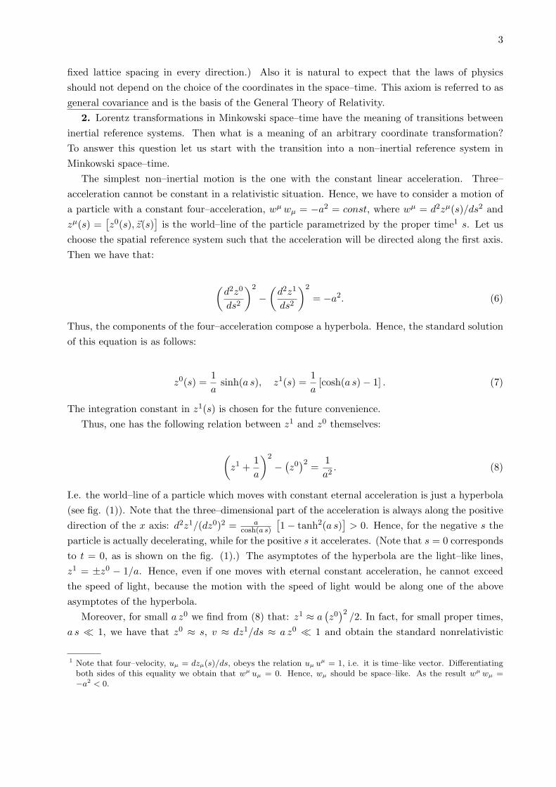
I.e. the world–line of a particle which moves with constant eternal acceleration is just a hyperbola(see fig. (1)). Note that the three–dimensional part of the acceleration is always along the positivedirection of the x axis: d2z1/(dz0)2 = a

cosh(a s)

[1− tanh2(a s)

]> 0. Hence, for the negative s the

particle is actually decelerating, while for the positive s it accelerates. (Note that s = 0 correspondsto t = 0, as is shown on the fig. (1).) The asymptotes of the hyperbola are the light–like lines,z1 = ±z0 − 1/a. Hence, even if one moves with eternal constant acceleration, he cannot exceedthe speed of light, because the motion with the speed of light would be along one of the aboveasymptotes of the hyperbola.

Moreover, for small a z0 we find from (8) that: z1 ≈ a(z0)2/2. In fact, for small proper times,

a s 1, we have that z0 ≈ s, v ≈ dz1/ds ≈ a z0 1 and obtain the standard nonrelativistic

1 Note that four–velocity, uµ = dzµ(s)/ds, obeys the relation uµ uµ = 1, i.e. it is time–like vector. Differentiatingboth sides of this equality we obtain that wµ uµ = 0. Hence, wµ should be space–like. As the result wµ wµ =−a2 < 0.

4

Figure 1: In this picture and also in the other pictures of this lecture we show only slices of fixed y and z.

acceleration, which, however, gets modified according to (8) once the particle reaches high enoughvelocities. It is important to stress at this point that eternal constant acceleration is physically im-possible due to the infinite energy consumption. I.e. here we are just discussing some mathematicalabstraction, which, however, is helpful to clarify some important issues.

These observations will allow us to find the appropriate coordinate system for accelerated ob-servers. The motion with a constant eternal acceleration is homogeneous, i.e. accelerated observercannot distinguish any moment of its proper time from any other. Hence, it is natural to expectthat there should be static (invariant under both time–translations and time–reversal transforma-tions) reference frame seen by accelerated observers. Inspired by (7), we propose the followingcoordinate change:

t = ρ sinh τ, x = ρ cosh τ, ρ ≥ 0,

y′ = y, and z′ = z. (9)

Please note that these coordinates cover only quarter of the entire Minkowski space–time. Namely— the right quadrant. In fact, since cosh τ ≥ | sinh τ |, we have that x ≥ |t|. It is not hard to guessthe coordinates which will cover the left quadrant. For that one has to choose ρ ≤ 0 in (9).

Under such a coordinate change we have:

dt = dρ sinh τ + ρ dτ cosh τ, dx = dρ cosh τ + ρ dτ sinh τ. (10)

Then dt2 − dx2 = ρ2 τ2 − dρ2 and:

5

x

t

x=const

t=const

O

ρ=const

τ=const

Figure 2:

ds2 = dt2 − dx2 − dy2 − dz2 = ρ2 dτ2 − dρ2 − dy2 − dz2 (11)

is the so called Rindler metric. It is not constant, ||gµν || = Diag(ρ2,−1,−1,−1), but is time–independent and diagonal (i.e. static), as we have expected.

In this metric the levels of the constant coordinate time τ are straight lines t/x = tanh τ inthe x− t plane (or three–dimensional flat planes in the entire Minkowski space). The levels of theconstant ρ are the hyperbolas x2− t2 = ρ2 in the x− t plane. The latter ones correspond to world–lines of observers which are moving with constant four–accelerations equal to 1/ρ on a slice of fixedy and z. The hyperbolas degenerate to light-like lines x = ±t as ρ → 0. These are asymptotes ofthe hyperbolas for all ρ. As one takes ρ closer and closer to zero the corresponding hyperbolas arecloser and closer to their asymptotes. Note also that τ = −∞ corresponds to x = −t and τ = +∞— to x = t. As the result we get a change of the coordinate lattice, which is depicted on the fig.(2).

3. The important feature of the Rindler’s metric (11) is that it degenerates at ρ = 0. This is theso called coordinate singularity. It is similar to the singularity of the polar coordinates dr2 +r2dϕ2

at r = 0. The space–time itself is regular at ρ = 0. It is just flat Minkowski space–time at thelight–like lines x = ±t. Another important feature of the Rindler’s metric is that the speed of lightis coordinate dependent:

If ds2 = 0, then∣∣∣∣dρdτ

∣∣∣∣ = ρ, when dy = dz = 0. (12)

At the same time, in the proper coordinates the speed of light is just equal to one dρ/ds = dρ/ρdτ =1. Furthermore, as ρ → 0 the speed of light, dρ/dτ , becomes zero. This phenomenon is relatedto the fact that if an observer starts an eternal acceleration with a = 1/ρ, say at the momentof time t = 0 = τ , then there is a region in Minkowski space–time from which light rays cannotreach him. In fact, as shown on the fig. (2) if a light ray was emitted from a point like O itis parallel to the asymptote x = t of the world–line of the observer in question. As the result,the light ray never intersects with hyperbolas, i.e. never catches up with eternally accelerating

6

Figure 3:

observer. These are the reasons why one cannot extend the Rindler metric beyond the light–likelines x = ±t. The three–dimensional surface x = t of the entire Minkowski space–time is referredto as the future event horizon of the Rindler’s observers (those which are staying at the constantρ positions throughout their entire life time). At the same time x = −t is the past event horizonof the Rindler’s observers.

Note that if an observer accelerates during a finite period of time, then, after the moment whenthe acceleration is switched off his world–line will be a straight line, which is tangential to thecorresponding hyperbola. (I.e. the observer will continue moving with the gained velocity.) Theangle this tangential line has with the Minkowskian time axis is less that 45o. Hence, sooner orlater the light ray emitted from a point like O will actually reach such an observer. I.e. thisobserver does not have an event horizon.

Another interesting phenomenon which is seen by the Rindler’s observers is shown on the fig.(3). A stationary object, x = const, in Minkowski space–time cannot cross the event horizon ofthe Rindler’s observers during any finite period of the coordinate time τ . This object just slowsdown and only asymptotically approaches the horizon. Note that, as ρ → 0 a fixed finite portionof the proper time, ds = ρdτ , corresponds to increasing portions of the coordinate time, dτ . Recallalso that τ = −∞ corresponds to x = −t and τ = +∞ — to x = t.

All these peculiarities of the Rindler metric is the price one has to pay for the considerationof the physically impossible eternal acceleration. However, if one were transferring to a referencesystem of observers which are moving with accelerations only during finite proper times, then hewould obtain a non–stationary metric due to the inhomogeneity of such a motion.

7

The main lesson to draw from these observations is as follows. The physical meaning of a generalcoordinate transformation that mixes spatial and time coordinates is a transition to another, notnecessary inertial, reference system. In this case curves corresponding to fixed spatial coordinates(e.g. dρ = dy = dz = 0) are world–lines of (non–)inertial observers. As the result, the essence ofthe general covariance is that physical laws, in a suitable form/formualtion, should not depend onthe choice of observers.

4. If even in flat space–time one can choose curvilinear coordinates and obtain a non–trivialmetric tensor gµν(x), then how can one distinguish flat space–time from the curved one? Further-more, since we understood the physics behind the curvilinear coordinates in flat space–time, thenit is also natural to ask: What is the physics behind curved space–times? To start answering thesequestions in the following lectures let us solve here a simple problem.

Namely, let us consider a free particle moving in a space–time with a metric gµν(x). Let us findits world–line via the minimal action principle. If one considers a world–line zµ(τ) parametrized bya parameter τ (that, e.g., could be either a coordinate time or the proper one), then the simplestinvariant characteristic that one can associate to the world–line is its length. Hence, the naturalaction for the free particle should be proportional to the length of its world–line. The reason whywe are looking for an invariant action is that we expect the corresponding equations of motionto be covariant (i.e. to have the same form in all coordinate systems), according to the aboveformulated principle of general covariance.

If one approximates the world–line by a broken line consisting of a chain of small intervals, thenits length can be approximated by the expression as follows:

L =N∑i=1

√gµν [zi] [zi+1 − zi]µ [zi+1 − zi]ν , (13)

which follows from the definition of the metric. In the limit N →∞ and |zi+1 − zi| → 0 we obtainan integral instead of the sum. As the result, the action should be as follows:

S = −m∫ 2

1ds = −m

∫ τ2

τ1

dτ√gµν [z(τ)] zµ zν . (14)

Here z = dz/dτ . The coefficient of the proportionality between the action, S, and the length, L,is minus the mass, m, of the particle. This coefficient follows from the complementarity — fromthe fact that when gµν(x) = ηµν we have to obtain the standard action for the relativistic particlein the Special Theory of Relativity.

Note that the action (14) is invariant under the coordinate transformations, zµ → zµ(z), andalso under the reparametrizations, τ → f(τ), if one respects the ordering of points along theworld–line, df/dτ ≥ 0. In fact, then:

dτ

√gµν

dzµ

dτ

dzν

dτ= df

√gµν

dzµ

df

dzν

df.

8

Let us find equations of motion that follow from the minimal action principle applied to (14). Thefirst variation of the action is:

δS = −m∫ τ2

τ1

dτδ [gµν(z) zµ zν ]

2√z2

=

= −m∫ τ2

τ1

dτ√z2

2√z2√z2

[δgµν(z) zµ zν + gµν(z) δzµ zν + gµν(z) zµ δzν

]. (15)

Here we denote z2 ≡ gαβ(z) zαzβ . Using the fact that√z2 dτ =

√gµν dzµ dzν = ds we can change

in (15) the parametrization from τ to the proper time s. After that we integrate by parts in the lasttwo terms in the last line of (15). This way we get reed from the differentiation of δz: δz = d

dsδz.Then, using the Dirichlet boundary conditions, i.e. assuming that δz(s1) = δz(s2) = 0, we arriveat the following expression for the first variation of S:

δS = −m∫ s2

s1

ds

2

∂αgµν(z) δzα zµ zν −

d

ds

[gµν(z) zν

]δzµ − d

ds

[gµν(z) zµ

]δzν

=

= −m∫ s2

s1

ds

2

∂αgµνδz

α zµ zν − ∂αgµν zα zν δzµ − ∂αgµν zα zµ δzν − 2 gµν zµ δzν

=

= −m∫ s2

s1

ds

[12

(∂α gµν − ∂µgαν − ∂νgµα

)zµ zν − gµα zµ

]δzα. (16)

In these expressions z = dz/ds and also we have used that gµν zµ δzν = gµν δzµ zν because gµν =

gνµ. Taking into account that according to the minimal action principle δS should be equal to zerofor any δzα, we arrive at the following relation:

zµ + Γµνα(z) zν zα = 0, (17)

which is referred to as the geodesic equation. Here

Γµνα =12gµβ

(∂ν gαβ + ∂α gβν − ∂βgνα

)(18)

are the so called Christoffel symbols and gµβ is the inverse metric tensor, gµβ gβν = δµν .

Problems:

• Show that the metric ds2 = (1 + a h)2 dτ−dh2−dy2−dz2 (homogeneous gravitational field)also covers the Rindler space–time. Find the coordinate change from this metric to the oneused in the lecture.

• Find the coordinates which cover the lower and upper quadrants (complementary to thosewhich are covered by Rindler’s coordinates) of the Minkowski space–time.

9

• Find the coordinate transformation and the stationary (invariant only under time–translations, but not under time–reversal transformation) metric in the rotating referencesystem with the angular velocity ω. (See the corresponding paragraph in Landau–Lifshitz.)

• (*) Find the coordinate transformation and the stationary metric in the orbiting referencesystem, which moves on the radius R with the angular velocity ω.

• (*) Consider a particle which was stationary in an inertial reference system. Then its accel-eration was adiabatically turned on and kept finite for long period of time. And finally itsacceleration was adiabatically switched off. I.e. this particle for the beginning is stationarythen accelerates for a while, and finally proceeds its motion with a constant gained velocity.Find the world–line for such a motion. Find a metric which is seen by such observers.

• (*) Find the equation for geodesics in the non–Riemanian metric:

dsn = gµ1...µn(x) dxµ1 . . . dxµn .

(**) What kind of geometries (instead of the Minkowskian one) are there, if gµ1...µn hasonly constant (coordinate independent) components? (We know that in the case of constantmetrics with two indexes we can reduce them by coordinate transformations to one of thestandard forms — (1, 1, 1, 1), (−1, 1, 1, 1), (−1,−1, 1, 1) and etc.. What are the standardtypes of constant metrics with more indexes? Furthermore, in the case of Minkowsian signa-ture there is a light–cone, which allows one to specify which events are causally connected.What does one have instead of that in the case of constant metrics with more indexes?)

• (**) What kind of geometry (instead of the Minkowskian one) is there, if gµν =Diag(1, 1,−1,−1) instead of Minkowskian metric? What is there instead of the light–coneand causality?

Subjects for further study:

• Radiation of the homogeneously accelerating charges: What is the intensity seen by a distantinertial observer? What is the intensity seen by a distant co–moving non–inertial observer?What is the invariant energy loss of the homogeneously accelerating charge? Does a freefalling charge in a homogeneous gravitational field create a radiation? Does a charge, whichis fixed in a homogeneous gravitational field, create a radiation? (“Radiation from a Uni-formly Accelerated Charges”, D.G.Bouleware, Annals of Physics 124 (1980) 169.“On radiation due to homogeneously accelerating sources”, D.Kalinov, e-Print:arXiv:1508.04281)

• Action and minimal action principle for strings and membranes in arbitrary dimensions.(Gauge fields and strings, A.Polyakov, Harwood Academic Publishers, 1987.)

10

LECTURE IITensors. Covariant differentiation. Parallel transport. Locally Minkowskian reference system.

Curvature or Riemann tensor and its properties.

1. This lecture is rather formal. Here we answer some of the questions posed in the first lectureand also clarify the geometric meaning of the Christoffel symbols.

For the beginning let us recall what is tensor. Under a transformation xµ = xµ (xν) the space–time coordinates tautologically transform as:

dxµ =∂xµ

∂xνdxν . (19)

A vector Aµ is referred to as contravariant if it transforms, under the coordinate transformation,in the same way as coordinates do:

Aµ(x) =∂xµ

∂xνAν (x) . (20)

At the same time a vector Aµ is referred to as covariant if it transforms as a one–form:

Aµ(x) dxµ = Aν (x) dxν , then Aµ(x) =∂xν

∂xµAν (x) . (21)

With the use of the metric tensor gµν and its inverse, gµν gνα = δµα, one can map covariant indexesonto contravariant ones and back:

Aµ = gµν Aν , and Aµ = gµν Aν . (22)

In particular xµ = gµν xν .

Then, n–tensor with the corresponding number of covariant and contravariant indexes is thequantity, which changes under the coordinate transformations, as follows (l + k = n):

T ν1...νlµ1...µk(x) =

∂xα1

∂xµ1. . .

∂xαk

∂xµk∂xν1

∂xβ1. . .

∂xνl

∂xβlT β1...βlα1...αk

(x) . (23)

In principle the order of the upper and lower indexes is important, but to simplify this formula weignore this detail here. For example, for the metric we have that

ds2 = gµν(x) dxµdxν = gαβ (x) dxαdxβ , then gµν(x) =∂xα

∂xµ∂xβ

∂xνgαβ (x) . (24)

With the use of the metric tensor and its inverse tensor one also can rise and lower indexes ofhigher rank tensors: e.g., Tµνα gνβ = Tµ

βα. In the last equation we show that the order of indexesis important.

11

All these definitions are necessary to make contractions of tensors to transform also as tensors.For example, TµναβMβ

ν should transform as two–tensor and it does, if one uses the above defini-tions. In particular, the scalar product of two vectors AµBµ = AµBµ = gµν A

µBν = gµν AµBν

should be (and is) invariant. That is all essence and convenience of the tensor notations, becausethen every expression has obvious properties under the general coordinate transformations.

2. Now we are ready to define the covariant differential. The ordinary differential is defined as

∂νAµ dxν ≡ Aµ (x+ dx)−Aµ(x). (25)

We will frequently use several different notations for the ordinary differential: ∂Aµ

∂xν ≡ ∂νAµ ≡ Aµ,ν .

The problem with the ordinary differential, ∂νAµ, is that, despite the fact that it has two indexes,it does not transform as two–tensor. In fact,

Aα,β (x) =∂

∂xβ∂xα

∂xµAµ(x) =

∂xα

∂xµ∂xν

∂xβAµ,ν(x) +

∂2xα

∂xµ∂xν∂xν

∂xβAµ(x). (26)

It is the covariant differential of a vector Aµ which transforms as two–tensor. To define it let ussubtract a quantity δAµ from the ordinary differential:

DαAµ dxα = ∂αA

µ dxα − δAµ. (27)

We will frequently use different notations for the covariant differential: DαAµ ≡ Aµ;α. The geometric

interpretation of δAµ is as follows. The above problems with the ordinary differential are due tothe fact that to find it we subtract two vectors Aµ (x+ dx) and Aµ(x), which are defined at twodifferent points — x+ dx and x. To overcome these problems, one has to parallel transport Aµ(x)to the point x+ dx. That is exactly what the addition of δAµ does:

DαAµ dxα ≡ Aµ (x+ dx)− [Aµ(x) + δAµ(x)] . (28)

For small dx the quantity δAµ should be linear in dx and also in Aµ. Hence, we define it to havethe following form:

δAµ(x) ≡ −Γµνα(x)Aν(x) dxα, (29)

where Γµνα(x) is referred to as the connection.As is seen from (26) and (28) for DαA

µ to be a two–tensor the connection Γµνα should transformas:

Γµνα(x) = Γβγσ (x)∂xµ

∂xβ∂xγ

∂xν∂xσ

∂xα+

∂2xγ

∂xν∂xα∂xµ

∂xγ. (30)

12

At the same time scalar product should not change under the parallel transport. Hence, fromδ (AµBµ) = 0 we have that:

Bµ δAµ = −AµδBµ = Aµ ΓµναBν dxα, (31)

where to obtain the last equality we used eq. (29) for δBµ. Because (31) should be valid for anyBµ, we have that:

δAµ = Γνµα(x)Aν(x) dxα, (32)

in addition to (29).As the result we have the following definition of the covariant derivative:

Aµ;α ≡ DαAµ = ∂αA

µ + ΓµναAν = (∂α δµν + Γµνα) Aν ,

Aµ;α ≡ DαAµ = ∂αAµ − ΓνµαAν =(∂α δ

νµ − Γνµα

)Aν . (33)

Similarly, the covariant differential of higher rank tensors is as follows:

Aµν;α = DαAµν = ∂αA

µν + ΓµβαAβν + ΓνβαA

µβ ,

Aµν;α = DαAµν = ∂αA

µν + ΓµβαA

βν − ΓβναA

µβ ,

Aµν;α = DαAµν = ∂αAµν − ΓβµαAβν − ΓβναAµβ, etc.. (34)

Along with Γµνα we will use:

Γβ| να = gβµ Γµνα. (35)

It is instructive to have in mind that for Minkowski metric, ηµν , one has that Γµνα = 0.3. For the future convenience here we define the Locally Minkowskian Reference System

(LMRS). It is such a reference frame in a vicinity of an arbitrary point x0 in which

gµν(x0) = ηµν , and Γαβγ(x0) = 0, (36)

but it does not mean that the derivatives of gµν and Γµνα are vanishing. Below we will see thecondition when it is impossible to put the derivatives to zero.

Let us discuss under what conditions one can fix such a gauge as (36). We put x0 to the originof two reference systems — of an original one, K, and of a new, K, reference system. Then, ifξ = x− x0 and ξ = x− x0, we can expand:

ξα = Aαβ ξβ +

12Bαβγ ξ

β ξγ +O(ξ3). (37)

13

where Aµν and Bµνα are some constant tensor parameters. Note that Bα

βγ = Bαγβ .

Under such a transformation we have that:

gαβ(x0) = AµαAνβ gµν(x0) +O(ξ),

Γαβγ(x0) = Aαµ Aνβ A

σγ Γµνσ(x0)−Bα

µν Aµβ A

νγ +O(ξ). (38)

Using 16 components of Aµα we can always solve 10 equations gµν(x0) = ηµν . The remaining 6parameters of Aµν correspond to the 3 rotations and 3 Lorentz boosts, under which the Minkowskianmetric tensor, ηµν , does not change. Furthermore, one can put Γµνσ(x0) = 0 by choosing Bα

µν =Aαγ Γγµν(x0).

4. Let us define now the so called torsion:

Sµνα ≡ Γµνα − Γµαν . (39)

According to (30) it transforms under the coordinate transformations as a three–tensor. If one canchoose LMRS at any point x, he obtains that Sµνα = 0, because Γµνα = 0. But, Sµνα transforms asa tensor, i.e. multiplicatively. Hence, if its components are smooth functions, then this tensor isalso zero in any other reference system. Due to the arbitrariness of the point x, we conclude thatif the metric is smooth enough and the gauge LMRS is possible, then

Γµνα = Γµαν , (40)

i.e. the connection is symmetric under the exchange of its lower indexes. Manifolds with vanishingtorsion are referred to as Riemanian.

5. Here we express the connection via the metric tensor. For the beginning we show that anymetric tensor should be covariantly constant. In fact,

DαAµ = Dα (gµν Aν) = (Dαgµν) Aν + gµν DαAν . (41)

But DαAµ is two–tensor. Hence, by the definition of the relation between covariant and contravari-ant indexes, we should have that DαAµ = gµν DαA

ν . Hence, from (41) it follows that the metrictensor should be covariantly constant: Dαgµν = 0. Using (34) and (35), we can write this conditionas:

gµν;α ≡ Dαgµν = ∂αgµν − Γµ| να − Γν|µα = 0. (42)

Reshuffling the indexes in this equation we also find that:

∂νgαµ − Γα|µν − Γµ|αν = 0,

∂µgνα − Γα| νµ − Γν|αµ = 0. (43)

14

Then, using the obtained system of three linear algebraic equations on Γµνα and the identity (40),we find the relation between the connection and the metric tensor:

Γα|µν =12

(∂ν gαµ + ∂µ gνα − ∂α gµν

), (44)

or

Γαµν =12gαβ

(∂ν gβµ + ∂µ gνβ − ∂β gµν

). (45)

Thus, for Riemanian manifolds the connection Γµνα coincides with the Christoffel symbols definedin the previous lecture.

As the result, the geodesic equation found in the previous lecture acquires a clear geometricmeaning,

[d

dsδµα + Γµνα [z(s)] uν(s)

]uα(s) = uν(s)Dνu

µ(s) = 0, (46)

as the condition of the covariant constancy of the four velocity uµ = dzµ/ds along the geodesicpath. In fact, uαDαu

µ is just the projection of the covariant derivative Dαuµ on to the tangent

vector uα to the geodesic.6. Now we define the curvature or Riemann tensor. Let us consider parallel transports of a

vector vµ from a point A to a nearby point C along two different infinitesimal paths — ABC andADC, as is shown on the fig. (4).

If one parallel transports vµ from A to B, then he finds:

vµAB ≈ vµ − Γµνα (A) vν ∆1x

α. (47)

Here Γµνα (A) is the value of the Christoffel symbol at the point A. Then,

Γµνα (B) ≈ Γµνα (A) + ∂β Γµνα (A) ∆1xβ . (48)

Now making further parallel transport from the point B to C, we find:

vµABC ≈ vµAB − Γµνα (B) vνAB ∆2x

α ≈

≈ vµ − Γµνα (A) vν ∆1xα −

[Γµνα (A) + ∂βΓµνα (A) ∆1x

β] [vν − Γνβδ (A) vβ ∆1x

δ]

∆2xα ≈

≈ vµ − Γµνα vν ∆1x

α − Γµνα vν ∆2x

α − ∂βΓµνα vν ∆1xβ ∆2x

α + Γµνα Γνβγ vβ ∆1x

γ ∆2xα. (49)

Similarly doing the parallel transport along the ADC path, one finds:

vµADC ≈ vµ − Γµνα v

ν ∆2xα − Γµνα v

ν ∆1xα − ∂βΓµνα vν ∆1x

α ∆2xβ + Γµνα Γνβγ v

β ∆1xα ∆2x

γ . (50)

15

Figure 4:

Then the difference between the two results of the parallel transport vµABC and vµADC is given by:

vµABC − vµADC ≈ −

[∂αΓµνβ − ∂βΓ

µνα + Γµγα Γγνβ − Γµγβ Γγνα

]vν ∆1x

α ∆2xβ ≡

≡ −12Rµναβ v

ν ∆Sαβ , (51)

where we have defined ∆Sαβ = ∆1xα ∆2x

β −∆1xβ ∆2x

α, which is the area of the parallelogramshown on the fig. (4), and

Rµναβ ≡ ∂αΓµνβ − ∂βΓµνα + Γµγα Γγνβ − Γµγβ Γγνα (52)

is the Riemann tensor that we have been looking for. The Riemann tensor is nothing but thecurvature for the connection in question:

Rµναβ =[Dµαγ , D

γβν

]≡ Dµ

αγ Dγβν −D

µβγ D

γαν , where Dµ

αν = ∂α δµν + Γµαν . (53)

One also uses the following form of this tensor: Rµναβ = gµγ Rγναβ .

Obviously in flat space–time vABC = vADC , hence the Riemann tensor is the measure of howthe space–time is curved. Note that the Riemann tensor transforms under the coordinate trans-formations multiplicatively. Hence, if it is zero in one reference system, then it is also zero in anyother system.

16

7. Let us specify the properties of the Riemann tensor. In a vicinity of any point x in LMRS(36) this tensor is equal to:

Rµναβ = ∂αΓµ| νβ − ∂βΓµ| να =12[∂2να gµβ − ∂2

νβ gµα − ∂2µα gνβ + ∂2

µβ gνα], (54)

where ∂2αβ = ∂α∂β and we also will be using the following notations: ∂2

αβ gµν = gµν, αβ . Now one cansee that if a space–time is curved, then even in the LMRS one cannot put to zero first derivativesof the Christoffel symbols and/or second derivatives of the metric tensor.

From (54) one immediately sees the following identities for the Riemann tensor:

Rµναβ = −Rνµαβ , Rµναβ = Rαβµν ,

Rµναβ +Rµαβν +Rµβνα = 0. (55)

Furthermore, differentiating (54), we find:

Rµναβ; γ +Rµνγα;β +Rµνβγ;α = 0, (56)

which is the so called Bianchi identity. Although we have obtained these identities in LMRS,they are valid for any reference system because they relate tensorial quantities, which changemultiplicatively under coordinate transformations.

A contraction of the Riemann tensor over any two of its indexes leads either to zero, Rααµν = 0(due to the anti-symmetry of Rµναβ under the exchange of the corresponding indexes), or to theso called Ricci tensor, Rµν ≡ Rαµαν . The latter one is symmetric Rµν = Rνµ tensor as theconsequence of (55). Contracting further the remaining two indexes, we obtain the Ricci scalar:R ≡ Rµν gµν . Furthermore, contracting two indexes in (56), we obtain the useful identity:

Rνµ; ν =12∂µR. (57)

8. Let us find the number of independent components of the Riemann tensor in aD–dimensionalspace–time. Riemann tensor Rµναβ is anti–symmetric under the exchanges µ←→ ν and α←→ β.Hence, the total number of independent combinations for each pair µν and αβ in D–dimensions isequal to D (D − 1)/2. On the other hand, Rµναβ is symmetric under the exchange of these pairs,µν ←→ αβ. Thus, the total number of independent combinations of the indexes is equal to

12D (D − 1)

2

[D (D − 1)

2+ 1]. (58)

However, we have to take into account the cyclic symmetry (the last equation in (55)):

Bµναβ = Rµναβ +Rµαβν +Rµβνα = 0. (59)

17

To find the number of these relations note that Bµναβ tensor is totaly anti–symmetric. For example,

Bµναβ = Rµναβ +Rµαβν +Rµβνα = −Rνµαβ −Rναβµ −Rνβµα = −Bνµαβ . (60)

Then, it is not hard to see that the total number of independent conditions, Bµναβ = 0, is equalto D (D − 1) (D − 2) (D − 3) /4!. As the result, the total number of independent components ofthe Riemann tensor is given by:

12D (D − 1)

2

[D (D − 1)

2+ 1]− D (D − 1) (D − 2) (D − 3)

4!=D2

(D2 − 1

)12

. (61)

In particular, in four dimensions we have 20 independent components, in D = 3 — 6 components,in D = 2 — only one.

In principle, around any given point we can further reduce the number of independent compo-nents of the Riemann tensor. In fact, LMRS around such a point is defined up to rotations andboosts, as we discuss above. Hence, with the appropriate choice of the parameters of the rotationone can put to zero D (D − 1) /2 more components of the Riemann tensor.

Problems

• Prove (53).

• Prove the Bianchi identity (56).

• Prove (57).

• Express the relative four–acceleration of two particles which move over infinitesimally closegeodesics via the Riemann tensor of the space–time. (See the corresponding problem in theLandau–Lifshitz.)


• Riemann, Ricci and metric tensors in three and two dimensions.

• Extrinsic curvatures of embedded lines and surfaces.

• Yang–Mills curvature and theory.

• Veilbein and spin connection. Riemann tensor via spin connection.

• Weyl tensor.

• Fermions and torsion.

18

LECTURE IIIEinstein–Hilbert action. Einstein equations. Matter energy–momentum tensor.

1. From the first two lectures we have learned about the physical meaning of arbitrary coor-dinate transformations and how to distinguish the flat space–time in cuverlinear coordinates fromcurved space–times. Now we are ready to address the question: What is the physics behind curvedspaces?

Set of experimental observations tells us that space–time is curved by anything that carriesenergy (originally this was a working guess, perhaps out of aesthetic considerations). Rephrasingthis, the metric tensor is a dynamical variable — a generalized coordinate — coupled to energycarried by matter. Our goal here is to see that all we need to formulate the theory of gravity isthis guess, general covariance and the minimal action principle. We would like to find equations ofmotion for the metric tensor, which relate so to say geometry of space–time to energy carried bymatter.

Obviously equations of motion that we are looking for should be covariant under general co-ordinate transformations, i.e. they should have the same form in all coordinate systems. Hence,the corresponding action for the metric should be invariant under these transformations. If wehave a metric tensor, then the simplest invariant that one can write is the volume of space–time,I =

∫ √|g| d4x, where |g| is the modulus of the determinant of the metric tensor, |det (gµν)|,

and d4x = dx0 dx1 dx2 dx3. It is alone is not suitable for the action, because it does not containderivatives of the metric. In fact, after the application of the minimal action principle to the ac-tion proportional to this invariant one will find an algebraic rather than differential (dynamical)equations of motion for the metric.

The simplest invariant that contains derivatives of the metric is the Ricci scalar, R = Rµα gµα =

gµα gνβ Rµναβ (see the previous lecture). Thus, the simplest invariant action for the metric aloneis as follows:

S = a

∫d4x

√|g|R+ b

∫d4x

√|g|, (62)

where a and b are some dimensionful constants, which one can fix only on the basis of experimentaldata. What remains to be added to this action is matter. Let SM be an action describing thecoupling of matter to gravity, i.e. to the metric tensor. We have encountered in the first lecturethe simplest example of such an action. That is the action for the point particle, SM = −m

∫ds =

−m∫dτ√gµν(z) zµ zν . But below we will also encounter other types of actions for matter. The

only thing about SM that we need to know at this point is that it should be invariant under thegeneral coordinate transformations.

All in all, we would like to apply the minimal action principle to the following action:

SEH = − 116πκ

∫d4x

√|g| (R+ Λ) + SM (gµν , matter) , (63)

19

which is referred to as the Einstein–Hilbert action. Here we have fixed the constants a and b in (62),knowing in advance their correct values. The quantity Λ is referred to as cosmological constant2

and κ is the seminal Newton’s constant.2. From the minimal action principle we have that

0 = δgSEH = − 116π κ

δg

∫d4x

√|g| (gµν Rµν + Λ) + δgSM =

= − 116π κ

∫d4x

[(δ√|g|)

(R+ Λ) +√|g| (δgµν) Rµν +

√|g| (δRµν) gµν

]+ δgSM . (64)

First, let us find δ√|g|. For that we derive here the generic identity:

δ log∣∣∣det M

∣∣∣ ≡ log∣∣∣det

(M + δM

)∣∣∣− log∣∣∣det M

∣∣∣ = logdet(M + δM

)det M

=

= log det[M−1

(M + δM

)]= log det

[1 + M−1 δM

]= Tr log

[1 + M−1 δM

]≈ TrM−1 δM.(65)

In this chain of relations M is a generic non–degenerate matrix and we have been keeping trace ofonly terms which are linear in δM .

Applying the obtained equation for gµν and its inverse tensor gµν we obtain:

δ log√|g| ≡ δ log

√|det (gµν)| = −

12δ log |det (gµν)| = −1

2gµν δg

µν .

Hence,

δ√|g| = −1

2

√|g| gµν δgµν . (66)

Second, let us continue with the term∫d4x

√|g| δRµν gµν in (64). In the LMRS, where gµν(x) =

ηµν and Γµνα(x) = 0, we have that:

δRµν = δ(Γαµν ,α − Γαµν ,ν

)= ∂α

(δΓαµν

)− ∂ν

(δΓαµα

)= Dα

(δΓαµν

)−Dν

(δΓαµα

). (67)

The last expression here is two tensor. Hence, we have a tensor relation between δRµν and δΓµνα,which is valid in any reference system, although it was obtained in LMRS. Thus,

gµν δRµν = Dµ

(gαβ δΓµαβ − g

αµ δΓβαβ)≡ DµδU

µ (68)

2 Quantum field theory predicts that Λ should be huge due to so called zero point fluctuations of quantum fields.At the same time, observational data show that Λ is not zero due to so called dark energy, but is very small. Thiscontradiction is the essence of the so called cosmological constant problem. For us, however, in these lectures,which are directed mostly to mathematicians and mathematical physicists, Λ is just an arbitrary parameter in thetheory, whose choice is at our disposal.

20

is a total covariant derivative of a four–vector δUµ. As the result,

∫Md4x

√|g| gµν δRµν =

∫Md4x

√|g|DµδU

µ =∮∂M

dΣµ δUµ, (69)

where M is the space–time manifold under consideration and ∂M is its boundary. To obtain thelast equality, we have used the Stokes’ theorem and dΣµ is the four–vector normal to ∂M, whosemodulus is the infinitesimal volume element of ∂M: dΣµ = nµ

√g(3) d3ξ, where nµ is the normal

vector to the boundary, g(3) = |det gij | is the determinant of the induced three–dimensional metric,gij , i = 1, 2, 3, on the boundary ∂M and ξ are the corresponding coordinates parametrizing theboundary.

Consideration of the boundary contributions is a separate interesting subject, but herewe are varying the action with such conditions that are as follows δUµ|∂M = 0. Hence,∫d4x

√|g| gµν δRµν = 0. Combining in (64) this fact together with (66), we find:

0 = δgSM −1

16π κ

∫d4x

√|g|(Rµν −

12gµν R−

12gµν Λ

)δgµν . (70)

What remains to be found is δgSM .3. Let us assume that the matter action, being invariant under the general coordinate trans-

formations, has the following form SM =∫d4√|g| L, where L is an invariant Lagrangian density.

For example,

∫ds =

∫dτ√gµν(z) zµ zν =

∫d4x

√|g(x)|

∫dτ

δ(4) [x− z(τ)]√|g(z)|

√gµν(z) zµ zν . (71)

The other examples will be given below.Then,

δgSM = δ

∫d4x

√|g| L =

∫d4x

[∂L∂gµν

δgµν√|g|+ L δ

√|g|]

=

=∫d4x

√|g|[∂L∂gµν

− 12L gµν

]δgµν ≡ 1

2

∫d4x

√|g|Tµν δgµν , (72)

where we have introduced a new two–tensor:

Tµν = 2∂L∂gµν

− L gµν , Tµν = Tνµ. (73)

Let us clarify the physical meaning of Tµν . Among the variations of the metric δgµν there are so tosay physical ones, which lead to the curvature variations of space–time, i.e. for them δRµναβ 6= 0.But there are also such variations of the metric tensor which are due to the trivial coordinatechanges, i.e. for them δRµναβ = 0. Let us specify the form of the latter variations. Under generalcoordinate transformations the inverse metric tensor transforms as:

21

gµν (x) = gαβ(x)∂xµ

∂xα∂xν

∂xβ. (74)

We are looking for the infinitesimal form of this transformation. If xµ = xµ + εµ(x), where εµ(x)is a small vector field, then:

gµν (x) ≈ gαβ(x) (δµα + ∂αεµ)(δνβ + ∂βε

ν)

= gµν(x) + ∂µεν + ∂νεµ ≡ gµν(x) + ∂(µεν). (75)

Taking into account that

gµν (x) = gµν (x+ ε) ≈ gµν(x) + ∂αgµν(x) εα, (76)

we find that at the linear order:

δεgµν ≡ gµν(x)− gµν(x) ≈ −∂αgµν εα + ∂(µεν) = D(µεν). (77)

Under such variations of the metric the action SM should not change at all, because it is aninvariant, as we agreed above. Hence, using (72), we obtain

0 ≡ δεSM =12

∫Md4x

√|g|Tµν D(µεν) =

∫Md4x

√|g|Tµν Dµεν =

=∫Md4x

√|g|Dµ (Tµν εν)−

∫Md4x

√|g| εν (Dµ Tµν) =

=∮∂M

dΣµ Tµν εν −

∫Md4x

√|g| εν (Dµ Tµν) , (78)

where we have used the symmetry Tµν = Tνµ, performed the integration by parts and used theStokes’ theorem. We assume vanishing variations at the boundary, εµ|∂M = 0. Then, becauseδεSM should vanish at any εµ insideM, we obtain the identity:

DµTµν = 0, (79)

which is a covariant generalization of a conservation law. In fact, in flat space it reduces to∂µTµν = 0, which is a conservation law following from the Nether’s theorem applied to coordinatetransformations. Thus, Tµν is nothing but the energy momentum tensor.

4. All in all, from (72) and (70) we obtain the Einstein equations:

Rµν −12Rgµν −

12

Λ gµν = 8π κTµν , (80)

which relate the geometry of space–time (left hand side) to the energy (right hand side).

22

In the vacuum Tµν = 0 and Λ = 0. Hence, we obtain the equation

Rµν −12Rgµν = 0. (81)

Multiplying it by gµν and using that gµν gνµ = δµµ = 4, we find that it implies R = 0, i.e. thisequation is equivalent to the Ricci flatness condition:

Rµν = 0. (82)

Note that this equation is not equivalent to the condition of vanishing of the curvature of space–timeRµναβ = 0. In the following lectures we will find vacuum solutions (with Tµν = 0 and Λ = 0) of theEinstein equations which are Ricci flat, but are not Riemann flat, i.e. describe curved space–times.

If we apply covariant differential Dν to both sides of eq. (80) and use the covariant constancyof the metric tensor Dαgµν = 0, we find that

Rνµ ;ν −12∂µR = 8π κDνTµν (83)

Using the consequence of the Bianchi identity Rνµ ;ν = 12 ∂µR, which was derived in the previous

lecture, we find the energy momentum tensor conservation condition, DνTµν = 0. Thus, even ifwe do not assume from the very beginning that Tµν is conserved, this condition follows from theEinstein equations and the Bianchi identity.

This situation is similar to the one we encounter in the case of Maxwell equations. In fact, ifone applies ∂ν derivative to the equation ∂µFµν = 4π jν , where Fµν = ∂µAν −∂νAµ and jν is four-current, he finds the continuity equation ∂µjµ = 0 due to anti–symmetry of the electromagnetictensor Fµν = −Fνµ. The continuity equation is just the condition of the charge conservation.However, from the dynamical point of view the conservation of the energy momentum tensormeans much more than the conservation of the electric current. Let us show that conservation ofTµν implies the equations of motion for matter.

Consider, for example, energy momentum tensor for a dust (cloud of free particles which donot create any pressure). As follows from the solution of the problems at the end of this lecture,in this case Tµν(x) = ρ(x)uµ(x)uν(x), here ρ(x) is the mass density of the dust and uµ(x) is itsfour–velocity vector field. (Note that in the reference frame where uµ = (1, 0, 0, 0) we obtain that||Tµν || = Diag(ρ, 0, 0, 0).) Let us consider the condition of the conservation of such an energymomentum tensor:

0 = Dµ (ρ uµuν) = (Dµρuµ) uν + ρ uµDµuν . (84)

Multiplying this equation by uν and using that uνuν = 1 (hence, Dµuνuν = 2uνDµuν = 0),

we obtain a covariant generalization, Dµ (ρ uµ) = 0, of the ordinary mass continuity equation∂µ (ρ uµ) = 0. Moreover, as the consequence of this equation from (84) we obtain that uµDµuν = 0.

23

Which means that species of the dust should move along geodesic curves, as the consequence of theenergy–momentum tensor conservation. Thus, Einstein equations necessarily imply the dynamicalequations of motion for matter. We will frequently encounter the consequences of these observationsin the following lectures.

5. Let us describe various simple examples of matter coupling to gravity, i.e. various examplesof SM . Consider e.g. a real scalar field φ. Then, the simplest invariants that one can write arepowers of φ. At the same time, the simplest invariant that contains derivatives of φ is gµν ∂µφ∂νφ.As the result the simplest action describing the coupling of the scalar field to the gravity is asfollows:

SM =∫d4x

√|g| [gµν ∂µφ∂νφ− V (φ)] , (85)

where V (φ) is a polynomial in φ.Let us continue now with the curved space–time generalization of the Maxwell theory. The

natural covariant generalization of the electromagnetic tensor is:

Fµν = DµAν −DνAµ = ∂µAν − ∂νAµ. (86)

As one can see this tensor does not change in passing from the flat space–time to a curved one. Asthe result, the curved space–time generalization of the Maxwell’s action

SM =∫d4x√|g|Fµν Fαβ gµα gνβ , (87)

is a trivial extension of the flat space action.

Problems

• Find the Tµν tensor for a collection of N free particles (i.e. for the dust):

SM = −N∑q=1

mq

∫dτq

√gµν(zq) z

µq zνq . (88)

Find the mass density ρ in this case.

• Find equations of motion (δφSM = 0 and δASM = 0) and Tµν for (85) and (87).

• Propose an invariant action for the metric, which is more complicated than the Einstein–Hilbert action. E.g. that which contains higher derivatives of the metric tensor. (*) Derivethe corresponding equations of motion.

24

• Prove the last equality in (77).


• The minimal action principle for space–times with boundaries (with variations of the metricat the boundary). Boundary terms.

• Different types of energy conditions for Tµν , their origin and meaning.

• Raychaudhuri equations.

• Veilbein formalism and spin connection.

• Three–dimensional gravity and the Chern–Simons theory. (See e.g. “Quantum gravity in2+1 dimensions: The Case of a closed universe”, S.Carlip, Living Rev.Rel. 8 (2005) 1; arXiv:gr-qc/0409039.)

• Two–dimensional gravity and Liouville theory. (Gauge fields and strings, A.Polyakov, Har-wood Academic Publishers, 1987.)

25

LECTURE IVSchwarzschild solution. Schwarzschild coordinates. Eddington–Finkelstein coordinates.

1. Starting with this lecture we look for solutions of the Einstein equations. One of the simplestexact solutions of these equations was found by Schwarzschild. It describes spherically symmetricgeometry when the cosmological constant is set to zero, Λ = 0, and in the absence of matter,Tµν = 0.

To find spherically symmetric geometry it is convenient to use spherical spatial coordinates,xµ = (t, r, θ, ϕ), instead of the Cartesian ones, xµ = (t, x, y, z), and to use the most generalspherically symmetric ansatz for the metric:

ds2 = gtt(r, t) dt2 + 2 gtr(r, t) dtdr + grr(r, t) dr2 + k(r, t) dΩ2,

where dΩ2 = dθ2 + sin2 θ dϕ2, and r ∈ [0,+∞) ϕ ∈ [0, 2π), θ ∈ [0, π]. (89)

Of course if one will choose a different coordinate frame (i.e. if one will make a generic coordi-nate change to an arbitrary reference system), then the spherical symmetry will be lost, but it isimportant to stress that there is a reference system in which the metric has the above form. Thisform of the metric is spherically symmetric because at a given moment of time, dt = 0, the spaceitself is sliced as an onion by spheres of radii following from grr(r, t) and whose areas are set up byk(r, t).

The form of the metric (89) is invariant under the following two–dimensional coordinate changes:r = r (r, t) , t = t (r, t). In fact, then:

gab (x) = gcd(x)∂xc

∂xa∂xd

∂xb, and k (x) = k [x (x)] ,

where xa = (r, t), a = 1, 2. (90)

Using this freedom of choice of two functions, r (r, t) and t (r, t), one can fix two out of the four func-tions, gtt(r, t), gtr(r, t), grr(r, t) and k(r, t). Without loss of generality in the case of nondegeneratemetric it is convenient to set grt = 0 and k(r, t) = −r2.

Then, introducing the standard notations gtt = eν(r,t) and grr = −eλ(r,t), we arrive at thefollowing convenient ansatz for the Einstein equations:

ds2 = eν(r,t) dt2 − eλ(r,t) dr2 − r2 dΩ2. (91)

It is important to note that the form of this metric is invariant under the remaining coordinatetransformations t = t (t). In fact, then

λ (r, t) = λ [r, t (t)] and ν (r, t) = ν [r, t (t)] + log(dt

dt

)2

. (92)

26

2. Thus, we have the following non-zero components of the metric and its inverse tensor:

||gµν || = Diag(eν ,−eλ,−r2,−r2 sin2 θ

), ||gµν || = Diag

(e−ν ,−e−λ,− 1

r2,− 1

r2 sin2 θ

). (93)

It is straightforward to find that non–zero components of the Christoffel symbols are given by:

Γ111 =

λ′

2, Γ0

10 =ν ′

2, Γ2

33 = − sin θ cos θ, Γ011 =

λ

2eλ−ν ,

Γ122 = −r e−λ, Γ1

00 =ν ′

2eν−λ, Γ2

12 = Γ313 =

1r,

Γ323 = cot θ, Γ0

00 =ν

2, Γ1

10 =λ

2, Γ1

33 = −r sin2 θ e−λ. (94)

For the metric ansatz under consideration the other components of Γµνα are zero, if they do notfollow from (94) via the application of the symmetry Γµνα = Γµαν . Here the prime on top of ν andλ means just the application of ∂/∂r differential and the dot — ∂/∂t.

As the result, the non–trivial part of the Einstein equations is as follows:

8π κT 11 = −e−λ

(ν ′

r+

1r2

)+

1r2,

8π κT 22 = 8π κT 3

3 = −12e−λ

(ν ′′ +

(ν ′)2

2+ν ′ − λ′

r− ν ′ λ′

2

)+

12e−ν

(λ+

λ2

2− λ ν

2

),

8π κT 00 = −e−λ

(1r2− λ′

r

)+

1r2,

8π κT 10 = −e−λ λ

r. (95)

Here for the future convenience we have written the Einstein equations in the form Rµν− 12 Rgµν =

8π κTµν , as if Tµν is not zero. The other part of the Einstein equations, corresponding to T 31 or

T 21 and etc., is trivially satisfied, if the corresponding components of Tµν are zero.

Now, if Tµν = 0, as we have assumed from the very beginning, then the equations under consid-eration reduce to:

e−λ(ν ′

r+

1r2

)− 1r2

= 0,

e−λ(λ′

r− 1r2

)+

1r2

= 0,

λ = 0. (96)

The equations for T 22 and T 3

3 in (95) follow from (96).From the third equation in (96) we immediately see that λ = λ(r) is time independent. Then,

taking the sum of the first and the second equation in (96), we obtain the relation λ′+ν ′ = 0, which

27

means that λ+ ν = g(t), where g(t) is some function of time only. Using the freedom (92) one canset this function to zero by appropriate change of ν. As the result, we obtain that ν = −λ(r).

Finally, it is not hard to solve the second equation in (96) to find that

e−λ = eν = 1 +C2

r. (97)

As r →∞ we restore the flat space–time metric

ds2 =(

1 +C2

r

)dt2 − dr2

1 + C2r

− r2 dΩ2 −→ dt2 − dr2 − r2 dΩ2. (98)

In fact, on general physical grounds one can conclude that the geometry in question is createdby a spherically symmetric massive body outside itself, i.e. in that part of space–time whereTµν(x) = 0. (We discuss these points in grater detail in the lectures that follow.) Then it isnatural to expect that there should be flat space at the spatial infinity, where the influence ofthe gravitating center is negligible. General metrics obeying such a condition are referred to asasymptotically flat. (Actually, the precise definition of what is asymptotically flat space–time ismore complicated, but for brevity we do not discuss it here.)

Thus, asymptotically flat, spherically symmetric metric in the vacuum (when Tµν = 0 andΛ = 0) is static — time independent and diagonal. This is the essence of the Birkhoff theorem,which is discussed from various perspectives throughout most of the lectures that follow. Thistheorem is just a more complicated analog of the one stating that in Maxwell’s theory sphericallysymmetric solution, which tends to zero at spatial infinity, is also necessarily static. The latter isthe unique seminal solution describing the Coulomb potential created by a point like or sphericallydistributed charge. But Birkhoff theorem has deeper consequences, which will be discussed in thelectures that follow.

3. To find the value of C2 in (98) consider a probe particle which moves in the background inquestion. Let the particle be non–relativistic and traveling far away from the gravitating center.Then, as is we know from the course of classical mechanics, the action for such a particle shouldbe:

S ≈ −m∫ [

1− ~z2

2+ V (|~z|)

]dt, (99)

where V (|~z|) = V (r) is the Newton’s potential, i.e. V (r) = −κMr , M is the mass of the gravitating

center and∣∣∣~z∣∣∣ 1 is the velocity of the particle. At the same time we know that S = −m

∫ds.

Hence, there is the following approximate relation:

ds ≈

[1− ~z2

2+ V (r)

]dt, as r →∞ and

∣∣∣~z∣∣∣ 1. (100)

28

Then, at the linear order in ~z2 and V (r), we have

ds2 ≈ [1 + 2V (r)] dt2 − ~z2 dt2 = [1 + 2V (r)] dt2 − d~z2, as r →∞. (101)

As the result for the weak field, r →∞, we ought to obtain

gtt ≈ 1 + 2V (r) = 1− 2κMr

, (102)

i.e. from (98) we deduce that C2 = −2κM .All in all, we have found the so called Schwarzschild solution of the Einstein equations:

ds2 =(1− rg

r

)dt2 − dr2

1− rgr

− r2 dΩ2, where rg ≡ 2κM. (103)

We will discuss the physical meaning of this metric in greater detail in the next lecture. But letus point out here a few relevant points concerning the geometry under consideration.

4. The metric (103) is invariant under time translations t→ t+ const and time reversal t→ −ttransformation. Time slices, dt = 0, of this metric are themselves sliced by static spheres. As theresult, curves corresponding to dr = dθ = dϕ = 0 are world–lines of non–inertial observers thatare fixed over the gravitating center. (We say that Schwarzschild metric is seen by non–inertialobservers, which are fixed at various radii r and angles θ, ϕ over the gravitating body.) Note thatphysical distance between (r1, θ, ϕ) and (r2, θ, ϕ) is given by

∫ r2r1

dr1− rg

r

6= r2 − r1. There is theapproximate equality in the latter equation only in the limit as r1,2 →∞.

The metric (103) degenerates as r → rg: in fact, then gtt → 0 and grr → ∞. As we will seein a moment, this singularity of the metric is a coordinate (unphysical) one. It is similar to thesingularity of the Rindler’s metric at ρ = 0, which was discussed in the first lecture. Hence, theSchwarzschild coordinates r and t are applicable only for r > rg.

In fact, none of the invariants, which one can build from this metric are singular at r = rg.For example, the simplest invariant — the volume form — is equal to d4x

√|g| = r2 sin θ dr dθ dϕ

and is regular at r = rg. The Ricci scalar is zero, as follows from the Einstein equations. One canbuild up other invariants using the Riemann tensor. The non–zero components of this tensor forthe metric in question are given by:

R0101 =rgr3, R0202 =

R0303

sin2 θ= −rg (r − rg)

2 r2,

R1212 =R1313

sin2 θ=

rg2 (r − rg)

, R2323 = −rg r sin2 θ. (104)

Other nonzero components of Rµναβ are obtained by permutations of the indexes of (104) accordingto the symmetries of this tensor. Then it is straightforward to find one of the invariants:

Rµναβ Rµναβ =

3r2gr6, (105)

29

Figure 5:

which is regular at r = rg.5. Another way to see that the space–time (103) is regular at r = rg is to make a coordinate

transformation to such a metric tensor which is regular at this surface. Let us perform the followingtransformations:

ds2 =(1− rg

r

)dt2 − dr2

1− rgr

− r2 dΩ2 =(1− rg

r

) [dt2 − dr2(

1− rgr

)2]− r2 dΩ2 =

=(1− rg

r

) [dt2 − dr2∗

]− r2 dΩ2. (106)

Here we have introduced the so called tortoise coordinate r∗:

dr∗ =dr

1− rgr

, and r∗ = r + rg log∣∣∣∣ rrg − 1

∣∣∣∣ . (107)

We have fixed an integration constant in the relation between this coordinate, r∗, and the radiusr. So that r∗ ≈ r, as r →∞ and r∗ → −∞ as r → rg.

Now, if one introduces v = t+ r∗ and transforms from (t, r) to (v, r) coordinates in (106), thenhe finds the Schwarzschild space–time in the so called ingoing Eddington–Finkelstein coordinates:

ds2 =(1− rg

r

)dv2 − 2 dv dr − r2 dΩ2. (108)

The obtained form of the metric tensor is not singular at r = rg and can be extended to r ≤ rg.

30

In the Eddington–Finkelstein coordinates the invariant (105) has the same from. Hence, wesee that the Schwarzschild space–time has a physical singularity at r = 0, i.e. the space–timein question is meaningful only beyond the point r = 0. Moreover, it is natural to expect thatEinstein’s theory brakes down as one approaches the point r = 0, where the curvature becomesenormous. The reason for that can be understood after the solution of the problem for the previouslecture, which addresses modifications of the Einstein–Hilbert action.

Let us consider the behavior of radial light–like geodesics in the metric (108). For them ds = 0and dθ = dϕ = 0. Then from (108) we find

[(1− rg

r

)dv − 2 dr

]dv = 0. (109)

From dv = 0 we obtain the ingoing light rays v ≡ t + r∗ = const. They are ingoing because ast→ +∞ we have to take r∗ → −∞ to keep v = const. At the same time, from

(1− rg

r

)dv = 2 dr

we obtain “outgoing” light rays. They are actually outgoing (r → +∞ as time goes by) only whenr > rg. These light rays evolve towards r → 0 when r < rg. The resulting picture is shown on thefig. (5). The thin lines are light–like geodesics. The arrows on these lines show the directions ofthe light propagation as one advances forward in time. The vertical line r = rg, dr = 0, on the fig.(5) is also one of the light–like geodesics.

Problems

• Derive (94) and components of Rµν from (91).

• Derive (105) from (104).

• Show that if in (106) one will introduce u = t − r∗ and transform from(t, r) to (u, r), he would find the Scwarzschild space–time in the so calledoutgoing Eddington–Finkelstein coordinates:

ds2 =(1− rg

r

)du2 + 2 du dr − r2 dΩ2. (110)

Show that this metric is mapped to (108) under the time reversal t→ −t.

• Show that if one will make the charge ρ =√

1− rgr in the Schwarzschild space–time, he

would obtain the metric, which in the vicinity of r = rg looks like:

ds2 ≈ ρ2 dt2 − (2 rg)2 dρ2 − r2g dΩ2, as ρ→ 0. (111)

Which is very similar to the Rindler space–time.

31

• Find the metric for the Schwarzschild space–time as seen by the free falling observers. (Seethe corresponding paragraph in Landau–Lifshitz.)


• Black hole and black brane solutions in higher and lower dimensional Einstein theories. (E.g.in “String Theory”, by J.Polchinski, Cambridge University Press, 2005.)

• Reissner–Nordstrom solution of the Einstein–Maxwell theory.

• Wormhole solutions. (See e.g. “Wormholes in spacetime and their use for interstellar travel:A tool for teaching general relativity”, M.S.Morris and Kip S.Thorne, Am. J. Phys. 56(5),May 1988.)

• Stability of the Schwarzschild solution under linearized perturbations. (See e.g. “The math-ematical theory of black holes”, S. Chandrasekhar, Oxford University Press, 1992)

32

LECTURE VPenrose–Carter diagrams. Kruskal–Szekeres coordinates. Penrose–Carter diagram for the

Schwarzschild black hole.

1. Let us discuss now the properties of the Schwarzschild solution on the so calledPenrose–Carter diagram. The idea of such a diagram is to select a relevant two–dimensional partof a space–time under consideration and to make its stereographic projection on a compact space.For two–dimensional spaces such a projection always possible via a conformal map. In fact, a two–dimensional metric tensor, being symmetric 2× 2 matrix, has 3 independent components. Two ofthem can be fixed using transformations of two coordinates. As the result any two–dimensionalmetric on R1,1 can be transformed to the following form gab = ω2(x) ηab, a = 1, 2. Here ω2(x) isa space–time dependent function, which is referred to as conformal factor. One just has to makesure that the corresponding coordinates, xa, take values in a compact range. The reason for thatwill be clear in a moment.

The main point behind the Penrose–Carter diagrams is that under conformal maps (when onedrops off the conformal factor) light–like world–lines and angles between them do not change.As the result one can clearly see causal properties of the original space–time on a compact dia-gram. The disadvantage of such diagram is that to draw it one has to know the whole space–timethroughout its entire history, which is frequently impossible in generic physical situations. MoreoverPenrose–Carter diagrams are sensitive only to global structure of space–time.

2. To illustrate these points let us draw the Penrose–Carter diagram for Minkowski space–time:ds2 = dt2 − dx2 − dy2 − dz2. Select e.g. (t, x) part of this space–time and make the followingtransformation t ± x = tan

(ψ±ξ

2

). Here if t, x ∈ (−∞,+∞), then ψ, ξ ∈ [−π, π]. Under such a

coordinate transformation the Minkowskian metric changes as follows:

dt2 − dx2 =1[

2 cos(ψ+ξ

2

)cos(ψ−ξ

2

)]2 [dψ2 − dξ2]. (112)

The conformal factor of the new metric,[

1

2 cos(ψ+ξ2 ) cos(ψ−ξ

2 )

]2

, blows up at |ψ ± ξ| = π, which

makes the boundary of the compact (ψ, ξ) space–time infinitely far away from any its internalpoint. This fact allows one to map the compact (ψ, ξ) space–time onto the non–compact (t, x)space–time.

Furthermore, it is not hard to see that equality dt2 − dx2 = 0 implies also that dψ2 − dξ2 = 0,and vise versa. Hence, conformal factor is irrelevant in the study of the properties of the light–likeworld–lines — those which obey, ds2 = 0. The latter in (ψ, ξ) space–time are also straight linesmaking 45o angles with respect to the ψ and ξ axes. Then, let us just drop off the conformal factorand draw the compact (ψ, ξ) space–time. It is shown on the fig. (6).

On this diagram we show light–like rays by thin straight lines. The arrows on them show thedirection of the light propagation, as t → +∞. Furthermore, on this diagram I± represent the

33

Figure 6:

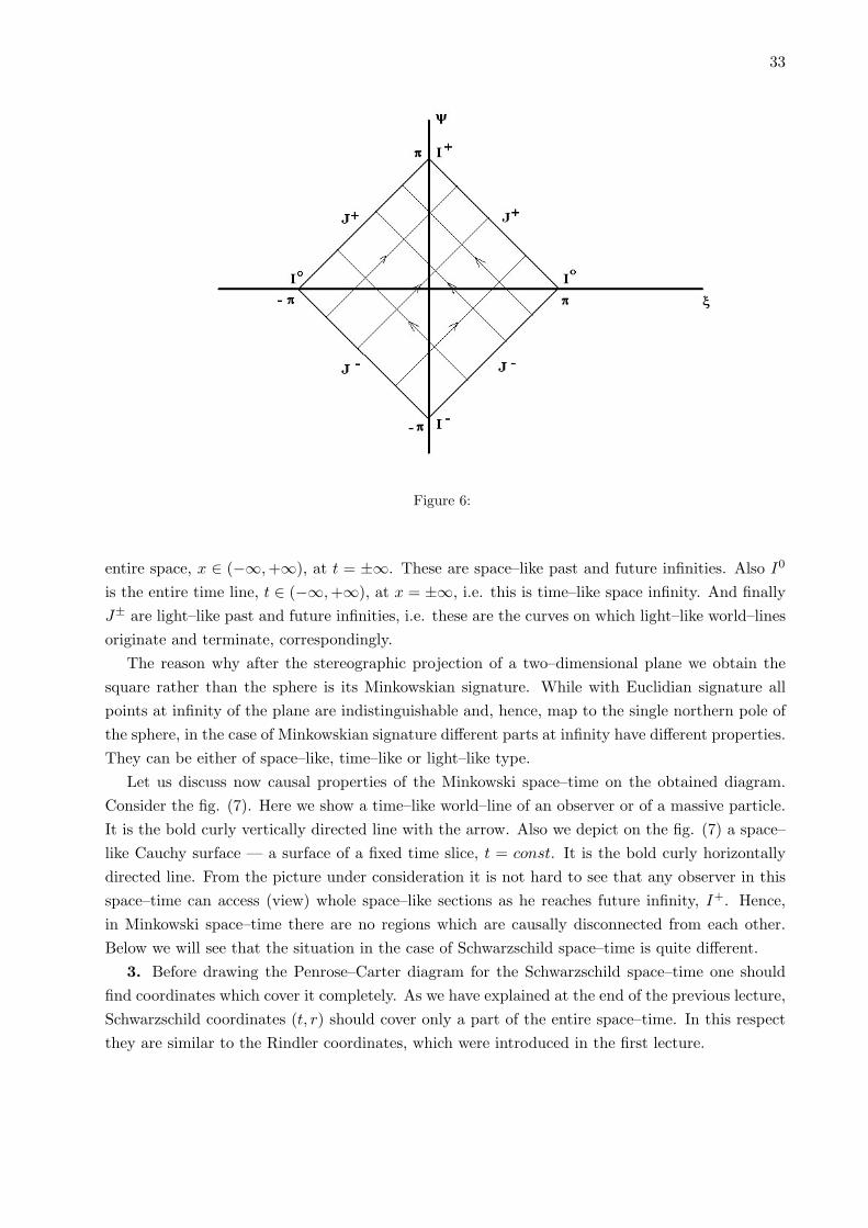
entire space, x ∈ (−∞,+∞), at t = ±∞. These are space–like past and future infinities. Also I0

is the entire time line, t ∈ (−∞,+∞), at x = ±∞, i.e. this is time–like space infinity. And finallyJ± are light–like past and future infinities, i.e. these are the curves on which light–like world–linesoriginate and terminate, correspondingly.

The reason why after the stereographic projection of a two–dimensional plane we obtain thesquare rather than the sphere is its Minkowskian signature. While with Euclidian signature allpoints at infinity of the plane are indistinguishable and, hence, map to the single northern pole ofthe sphere, in the case of Minkowskian signature different parts at infinity have different properties.They can be either of space–like, time–like or light–like type.

Let us discuss now causal properties of the Minkowski space–time on the obtained diagram.Consider the fig. (7). Here we show a time–like world–line of an observer or of a massive particle.It is the bold curly vertically directed line with the arrow. Also we depict on the fig. (7) a space–like Cauchy surface — a surface of a fixed time slice, t = const. It is the bold curly horizontallydirected line. From the picture under consideration it is not hard to see that any observer in thisspace–time can access (view) whole space–like sections as he reaches future infinity, I+. Hence,in Minkowski space–time there are no regions which are causally disconnected from each other.Below we will see that the situation in the case of Schwarzschild space–time is quite different.

3. Before drawing the Penrose–Carter diagram for the Schwarzschild space–time one shouldfind coordinates which cover it completely. As we have explained at the end of the previous lecture,Schwarzschild coordinates (t, r) should cover only a part of the entire space–time. In this respectthey are similar to the Rindler coordinates, which were introduced in the first lecture.

34

Figure 7:

To find coordinates which cover entire space–time one has to embed it as a hyperplane intoa higher–dimensional Minkowski space. Then one, in principle, can find such coordinates whichcover the hyperplane completely and, hence, they cover the entire original curved space–time.

At every point of a four–dimensional space–time its metric, being a symmetric two–tensor, hassix independent components. Hence, an arbitrary four–dimensional space–time can be embeddedlocally as a four–dimensional hyperplane into the ten–dimensional Minkowski space–time.

However, if a curved space–time has extra symmetries, then it can be embedded into a flatspace of a dimensionality less than ten. For example, Schwarzschild space–time, being quite sym-metric, can be embedded into six–dimensional flat space. This embedding is done with the use ofthe so called Kruskal–Szekeres coordinates. The machinery of such an embedding is beyond thescope of our concise lectures. We will present the Kruskal–Szekeres coordinates from a differentperspective. At this point the reader just has to believe us that the coordinates in question coverthe Schwarzschild space–time completely.

So let us start with the metric

ds2 =(1− rg

r

) (dt2 − dr2∗

)− r2 dΩ2, (113)

which is written in terms of the tortoise coordinate,

r∗ = r + rg log∣∣∣∣ rrg − 1

∣∣∣∣ . (114)

35

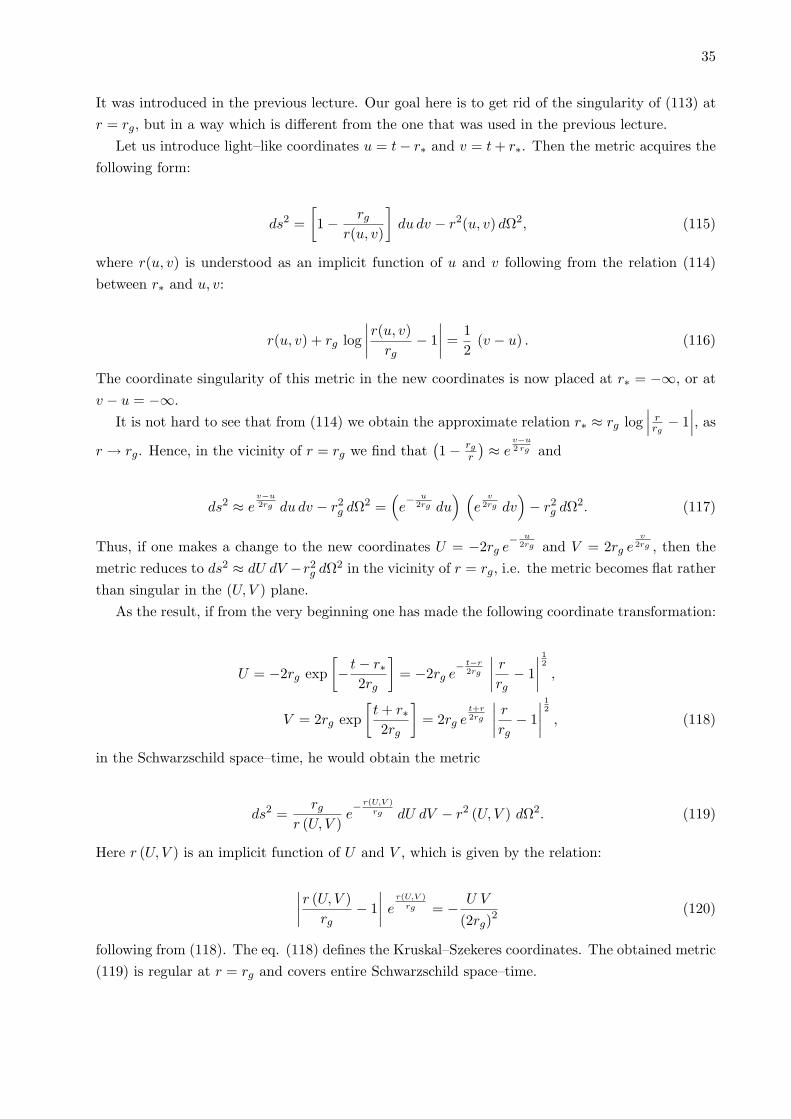
It was introduced in the previous lecture. Our goal here is to get rid of the singularity of (113) atr = rg, but in a way which is different from the one that was used in the previous lecture.

Let us introduce light–like coordinates u = t− r∗ and v = t+ r∗. Then the metric acquires thefollowing form:

ds2 =[1− rg

r(u, v)

]du dv − r2(u, v) dΩ2, (115)

where r(u, v) is understood as an implicit function of u and v following from the relation (114)between r∗ and u, v:

r(u, v) + rg log∣∣∣∣r(u, v)rg

− 1∣∣∣∣ = 1

2(v − u) . (116)

The coordinate singularity of this metric in the new coordinates is now placed at r∗ = −∞, or atv − u = −∞.

It is not hard to see that from (114) we obtain the approximate relation r∗ ≈ rg log∣∣∣ rrg − 1

∣∣∣, as

r → rg. Hence, in the vicinity of r = rg we find that(1− rg

r

)≈ e

v−u2 rg and

ds2 ≈ ev−u2rg du dv − r2g dΩ2 =

(e− u

2rg du) (

ev

2rg dv)− r2g dΩ2. (117)

Thus, if one makes a change to the new coordinates U = −2rg e− u

2rg and V = 2rg ev

2rg , then themetric reduces to ds2 ≈ dU dV −r2g dΩ2 in the vicinity of r = rg, i.e. the metric becomes flat ratherthan singular in the (U, V ) plane.

As the result, if from the very beginning one has made the following coordinate transformation:

U = −2rg exp[− t− r∗

2rg

]= −2rg e

− t−r2rg

∣∣∣∣ rrg − 1∣∣∣∣ 12 ,

V = 2rg exp[t+ r∗2rg

]= 2rg e

t+r2rg

∣∣∣∣ rrg − 1∣∣∣∣ 12 , (118)

in the Schwarzschild space–time, he would obtain the metric

ds2 =rg

r (U, V )e− r(U,V )

rg dU dV − r2 (U, V ) dΩ2. (119)

Here r (U, V ) is an implicit function of U and V , which is given by the relation:

∣∣∣∣r (U, V )rg

− 1∣∣∣∣ e r(U,V )

rg = − U V

(2rg)2 (120)

following from (118). The eq. (118) defines the Kruskal–Szekeres coordinates. The obtained metric(119) is regular at r = rg and covers entire Schwarzschild space–time.

36

Figure 8:

4. Let us describe the coordinate lattice in the new coordinates. Here we will discuss onlythe relevant two–dimensional, (U, V ), part of the space–time under consideration. From (120) onecan see that curves of constant r are hyperbolas in the (U, V ) plane. At r = rg these hyperbolasdegenerate to UV = 0, i.e. into two straight lines U = 0 and V = 0. At the same time from

V

U= e

trg (121)

one can deduce that curves of constant t are just straight lines.As the result the relation between (t, r) and (U, V ) coordinates is similar to the one we have

had in the first lecture between Rindler’s (τ, ρ) and Minkowskian (t− x, t+ x) coordinates. Notethat U and V are light–like coordinates, because equations dV = 0 and dU = 0 describe light rays.Having these relations in mind, one can understand the picture shown on the fig. (8).

As we have explained at the end of the pervious lecture the Schwarzschild space–time has aphysical singularity at r = 0. The two sheets of the corresponding hyperbola in (120) are depictedby the bold lines on the fig. (8). The Kruskal–Szekeres coordinates and space–time itself are notextendable beyond these curves. At the same time the Schwarzschild metric and (t, r) coordinatescover only quarter of the fig. (8), namely — the right quadrant.

5. To draw the Penrose–Carter diagram for the Schwarzschild space–time let us do exactly thesame transformation as at the beginning of this lecture. Let us transfrom from U ≡ T − X andV ≡ T + X to the ψ ± ξ coordinates and drop off the conformal factor. The resulting compact(ψ, ξ) space–time is shown on the fig. (9). This is basically the same picture as is shown on thefig. (6), but with chopped off two triangular pieces from the top and from the bottom.

37

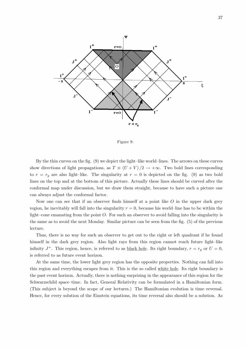
Figure 9:

By the thin curves on the fig. (9) we depict the light–like world–lines. The arrows on these curvesshow directions of light propagations, as T ≡ (U + V ) /2 → +∞. Two bold lines correspondingto r = rg are also light–like. The singularity at r = 0 is depicted on the fig. (9) as two boldlines on the top and at the bottom of this picture. Actually these lines should be curved after theconformal map under discussion, but we draw them straight, because to have such a picture onecan always adjust the conformal factor.

Now one can see that if an observer finds himself at a point like O in the upper dark greyregion, he inevitably will fall into the singularity r = 0, because his world–line has to be within thelight–cone emanating from the point O. For such an observer to avoid falling into the singularity isthe same as to avoid the next Monday. Similar picture can be seen from the fig. (5) of the previouslecture.

Thus, there is no way for such an observer to get out to the right or left quadrant if he foundhimself in the dark grey region. Also light rays from this region cannot reach future light–likeinfinity J+. This region, hence, is referred to as black hole. Its right boundary, r = rg or U = 0,is referred to as future event horizon.

At the same time, the lower light grey region has the opposite properties. Nothing can fall intothis region and everything escapes from it. This is the so called white hole. Its right boundary isthe past event horizon. Actually, there is nothing surprising in the appearance of this region for theSchwarzschild space–time. In fact, General Relativity can be formulated in a Hamiltonian form.(This subject is beyond the scope of our lectures.) The Hamiltonian evolution is time–reversal.Hence, for every solution of the Einstein equations, its time reversal also should be a solution. As

38

the result, in the static situation we simultaneously have the presence of both solutions.6. In the lectures that follow we will quantitatively describe the properties of the black holes in

grater details. But let us discuss some of these properties qualitatively here on the Penrose–Carterdiagram. Consider the fig. (10). On this diagram an observer, depicted as having number 3, isfixed on some radius above the black hole. (Number 3 also can rotate around the black hole on acircular orbit: Penrose–Carter diagram cannot distinguish these two types of behavior, because itis not sensitive to the change of spherical angles θ and ϕ.) Thus, the observer number 3 alwaysstays outside the black hole.

Then at some point another observer, e.g. number 1, starts his fall into the black hole from thesame orbit. As we will show in the lectures that follow he crosses the event horizon, r = rg, or evenreaches the singularity, r = 0, within finite proper time. At the same time from the diagram shownon the fig. (10), one can deduce that the observer number 3 never sees how the number 1 crossesthe event horizon. In fact, the last light ray which is scattered off by the number 1 goes along thehorizon and reaches the number 3 only at I+, i.e. at the future infinity. The situation is completelysimilar to the one which we have encountered in the first lecture for the case of Rindler’s metric.In fact, similarly to that case, the relation between the proper and coordinate time is as follows:

ds =(1− rg

r

) 12dt =

√g00 dt. (122)

Hence, fixed portions of the proper time, ds, correspond to the longer portions of the coordinatetime, dt, if one resides closer to the horizon, r → rg. Recall also that, as follows from (121),t = −∞ corresponds to V = 0 (past event horizon) and t = +∞ corresponds to U = 0 (futureevent horizon).

But the picture which is seen by another falling observer, shown as the number 2 on the fig.(10), which starts his fall after the number 1, is quite different. He never looses the number 1from his sight and sees him crossing the horizon. But the light rays which are scattered off by thenumber 1 before the crossing of the horizon are received by the number 2 also before he himselfcrosses the horizon. At the same time, after crossing the horizon the number 2 starts to receivethose light rays which are scattered off by the number 1 only after he crossed the horizon.

Problems

• Show the world line of an eternally accelerating observer/particle on the Penrose–Carterdiagram of the Minkowskian space–time, i.e. on the fig. (6).

• Which part of the black hole Penrose–Carter diagram is covered by the ingoing Edington–Finkelstein coordinates? Why?

• Which part of the black hole Penrose–Carter diagram is covered by the outgoing Edington–Finkelstein coordinates? Why?

39

Figure 10:

• Draw the Penrose–Carter diagram for (t, r) part of the Minkowskian space–time in thespherical coordinates: ds2 = dt2 − dr2 − r2 dΩ2.


• Kruskal’s embedding of the Schwarzschild solution into the six dimensional Minkowski space–time. (“Maximal extension of Schwarzschild metric”, M.D. Kruskal, Phys. Rev., Vol. 119,No. 5 (1960) 1743.)

• Cauchy problem in General Relativity and Hamiltonian formulation of the Einstein’s theory.Time reversal of the Hamiltonian evolution.

• Apparent horizon and other types of black hole horizons.

• Penrose and Hawking singularity theorems.

• Positive energy theorem, Penrose bound and their proof. (See e.g. “A new proof of thepositive energy theorem”, E. Witten, Commun. Math. Phys. 80, 381-402 (1981);“Theinverse mean curvature flow and the Riemannian Penrose inequality”, G. Huisken and T.Ilmanen, J. Differential Geometry 59 (2001) 353-437; “Proof of the Riemannian Penroseinequality using the positive mass theorem”, H.L. Bray, J. Differential Geometry 59 (2001)177-267)

40

• Asymptotic conformal infinity and asymptotically flat space–times.

• BondiMetznerSachs transformations.

• Newman–Penrose formalism.

41

LECTURE VIKilling vectors and conservation laws. Test particle motion on Schwarzschild black hole back-

ground. Mercury perihelion rotation. Light ray deviation in the vicinity of the Sun.

1. In this lecture we provide a quantitative approval of several qualitative observations thathave been made in the previous lectures. Furthermore, we derive from the General Theory ofRelativity some effects that have been approved by classical experiments.

As we have shown in one of the previous lectures, under an infinitesimal transformation,

xµ = xµ + εµ(x),

the inverse metric tensor transforms as

gµν(x) = gµν(x) +D(µεν)(x).

If for some of the transformations, εµ = kµ, the metric tensor does not change, i.e.

D(µkν) ≡ Dµkν +Dνkµ = 0, (123)

then the corresponding vector field, kµ, is referred to as Killing vector and the transformations arecalled isometries of the metric. For example, the Schwarzschild metric tensor does not depend ontime, t, and angle, ϕ. Hence, it’s isometries include at least the translations in time t → t + a

and rotations ϕ → ϕ + b, for some constants a and b. The corresponding Killing vectors, kµ =(kt, kr, kθ, kϕ

), have the following form: kµ = (1, 0, 0, 0) and kµ = (0, 0, 0, 1).

2. Here we show that if there is a Killing vector, then there also should be a conserved quantityas a revelation of the Noerther theorem. Consider a particle moving along a world–line zµ(s) withthe four–velocity uµ(s) ≡ dzµ/ds. Then, let us calculate the following derivative:

d

dskµuµ = ∂ν (kµuµ)

dzν

ds= kµ uν Dνuµ + uν uµDνkµ = kµ (uν Dνuµ) +

12uν uµ (Dν kµ +Dµ kν) .

If the particle moves along a geodesic, then uν Dνuµ = 0 and, if kµ is the Killing vector, thenDµkν + Dνkµ = 0. As the result, d(kµuµ)

ds = 0, i.e. the corresponding quantity is conserved,kµuµ = const.

3. Consider the Schwarzschild space–time and the Killing vector kµ = (1, 0, 0, 0). Then, theconserved quantity is given by

kµuµ = u0 = g00 u0 =

(1− rg

r

) dt

ds≡ E

m, (124)

where m is the mass of the particle and the physical meaning of E will be specified in a moment.

42

Similarly for the Killing vector kµ = (0, 0, 0, 1) we obtain the following conserved quantity:

r2 sin2 θdϕ

ds≡ L

m. (125)

The physical meaning of L will also be defined in a moment. As can be seen from this conservationlaw and similarly to the Newton’s theory, in radially symmetric space–times a trajectory of aparticle is restricted to a plane. In our case we choose such a plane to be at x3 = 0, i.e. at θ = π

2 .Hence, we can represent the last conserved quantity as r2 dϕ

ds = Lm .

Furthermore, in the background of the Schwarzschild metric the four–velocity should obey:

gµν uµ uν =

(1− rg

r

) ( dtds

)2

−(drds

)21− rg

r

− r2(dϕ

ds

)2

= 1, (126)

under the assumption that θ = π2 and, hence, dθ = 0. Using the two conservation laws that have

been derived above, we find that the world–line of a massive particle in Schwarzschild space–timeobeys the following equation:

(dr

ds

)2

=(E

m

)2

−(1− rg

r

) (1 +

L2

m2 r2

). (127)

To clarify the physical meaning of E and L, let us consider the Newtonian, rg r, and non–relativistic, dr/dt 1, limit of this equation. Then dr/ds ≈ dr/dt and:

E2 −m2

2m≈ m

2

(dr

dt

)2

+L2

2mr2− mrg

2r. (128)

If E2 −m2 = (E −m) (E +m) ≈ 2m E , where E = (E −m) m is the non–relativistic kineticenergy, and L is the angular momentum, then this equation defines the trajectory of a massiveparticle in the Newtonian gravitational field. Thus, as it should be, the conservation of energy, E,follows from the invariance under time translations and the conservation of the angular momentum,L, follows form the invariance under rotations.

4. For the radial infall into the black hole, L = 0, eq. (127) reduces to:

(dr

ds

)2

=(E

m

)2

−(1− rg

r

). (129)

Let us assume that dr/ds → 0, as r → ∞, i.e. the particle starts its free fall at infinity with thezero velocity. Then, as follows from (129), E = m and this equation simplifies to:

(dr

ds

)2

=rgr. (130)

43

From here one can deduce that the proper time of the particle’s free fall from a radius r = R tothe horizon r = rg is equal to:

s (R→ rg) = −∫ rg

R

(r

rg

) 12

dr =2 rg3

[(R

rg

) 32

− 1

]. (131)

The minus sing in front of the integral here is due to the fact that for the falling in trajectory —dr < 0 as ds > 0. Hence, as we have mentioned in the previous lectures, it takes a finite propertime for a particle or an observer to cross the black hole horizon.

At the same time, from (124) it follows that dt/ds = 1/(

1− rgr

), if E = m. Then, the ratio of

dr/ds by dt/ds leads to

dr

dt= −

(rgr

) 12(1− rg

r

). (132)

As the result, the Schwarzschild time, which is necessary for a particle to fall from a radius r =R rg to a radius r = rg + ε in the vicinity of the horizon, ε rg, is given by:

t (R→ rg + ε) = −∫ rg+ε

R

(r

rg

) 12 r dr

r − rg∼ rg log

R

ε. (133)

Hence, t → +∞, as ε → 0, and a particle cannot approach the horizon within finite time, asmeasured by an observer fixed over the black hole. This again coincides with our expectationsfrom the previous lectures.

5. Let us continue with the classical experimental approvals of the General Theory of Relativity.From the seminal Newton’s solution of the Kepler’s problem it is know that planets orbit alongellipsoidal trajectories around stars. How does this behavior change, if relativistic correctionsbecome relevant?

Using the above mentioned conservation laws, we can find that:

dr

ds=dr

dϕ

dϕ

ds=dr

dϕ

L

mr2= − L

m

du

dϕ, (134)

if the notation u = 1/r is introduced. Then, the equation (127) acquires the following form:

(du

dϕ

)2

+ u2 (1− rg u) =E2 −m2

L2+m2

L2rg u. (135)

Differentiating both sides of this equation by d/dϕ and dividing by du/dϕ, we obtain:

d2u

dϕ2+ u =

m2 rg2L2

+3 rg2

u2. (136)

44

In the Newtonian limit, rg/r = rg u 1, the last term in the obtained equation is negligible. Herewe discuss small deviations from the Newtonian gravitation and, hence, consider the term 3 rg

2 u2,on the right hand side of (136), as a perturbation.

Thus, in the Newtonian limit (136) reduces to

d2u0

dϕ2+ u0 =

m2 rg2L2

. (137)

The subscript “0” corresponds to the zero approximation in the perturbation over u rg 1. Thesolution of this oscillator type equation is given by:

u0 ≡1r0

=m2 rg2L2

(1 + e cosϕ) . (138)

If the eccentricity, e, is less than one, then the resulting trajectory is ellipse. As one can find from(136) the first correction, u1, obeys the following equation

d2u1

dϕ2+ u1 =

3 rg2

u20. (139)

Here:

3 rg2

u20 =

3 r3gm4

8L4(1 + e cosϕ)2 =

3 r3gm4

8L4+

3 r3gm4

4L4e cosϕ+

3 r3gm4

8L4e2 cos2 ϕ =

=3 r3gm

4

8L4

(1 +

e2

2

)+

3 r3gm4

4L4e cosϕ+

3 r3gm4

16L4e2 cos(2ϕ). (140)

The contribution 3 r3gm4

8L4

(1 + e2

2

)to u1 leads to a small correction of the m2 rg

2L2 factor in u0, i.e. in(137). This is just a small deviation of the length of the main axis of the ellipse, which is not avery interesting correction, because the main axis of the planetary ellipse in the Sun system cannotbe measured with such an accuracy.

We are looking for the largest correction to u0 coming from u1. This correction is provided by aresonant solution of (139). In this respect the last term, ∼ cos(2ϕ), in (140) leads to a suppressedresonant contribution to u1 in comparison with the term ∼ cosϕ, due to the mismatch of thefrequency of this “external force” with the frequency of the oscillator in (139).

All in all, to find the biggest correction u1 we just have to find the resonant solution of theequation:

d2u1

dϕ2+ u1 =

3 r3gm4

4L4e cosϕ. (141)

We look for the solution of this equation in the following form:

u1 = A(ϕ) sinϕ+B(ϕ) cosϕ, (142)

45

where A(ϕ) and B(ϕ) are slow functions. Such a u1 function solves (141), if:

A′′ = B′′ = 0, and 2A′ cosϕ− 2B′ sinϕ =3 r3gm

4

4L4e cosϕ. (143)

Wherefrom we find that B′ = 0 and A′ = 3 r3gm4

8L4 e. Hence, B = const and the correspondingcorrection is not resonant. As the result, the relevant for our considerations part of u0 + u1 is asfollows

u0 + u1 ≡1

r0+1≈ m2 rg

2L2(1 + e cosϕ) +

3 r3gm4 e

8L4ϕ sinϕ. (144)

The last term here was obtained under the assumption that it is just a small correction, i.e.3 r2gm

2

4L2 ϕ 1. Hence, eq. (144) can be rewritten as:

1r0+1

≈ m2 rg2L2

[1 + e cos

(ϕ−

3 r2gm2

4L2ϕ

)]. (145)

Now one can see that while the unperturbed trajectory is periodic in the standard sense, r0(ϕ) =r0(ϕ + 2π), a particle moving along the corrected trajectory returns back after the rotation overan angle, which is different from 2π

r0+1(ϕ) ≈ r0+1

(ϕ+ 2π +

3π r2gm2

2L2

).

Hence, due to relativistic effects the perihelion of a planet is rotated by the following angle

δϕ =3π r2gm

2

2L2, (146)

in one its period. Let us estimate this quantity for a circular orbit. In the latter case L = mvR

and v2 = rg2R , where R is the radius of the orbit and v is the planet’s velocity. Hence, δϕ ≈ 3π rg

R .At the same time for an elliptic orbit the same quantity is equal to δϕ ≈ 3π rg

R(1−e2).

If we substitute here the parameters of the Mercury orbit, which is the closest planet to theSun and, hence, is the most sensitive to the relativistic corrections, we obtain that δϕ ≈ 0, 1′′.However, this is the secular effect, i.e. grows with the number of times the planet rotates aroundthe Sun. During one hundred years the gained angle is equal to 43′′. This angle perfectly agreeswith the observational data.

6. Let us find now the deviation angle of a light ray passing in the vicinity of a massive body.For the light m = 0 and the equation (136) reduces to:

d2u

dϕ2+ u =

3 rg2

u2. (147)

46

Figure 11:

As before we consider the right hand side of this equation as a perturbation, u rg 1. Then, atzero approximation the equation has the following form:

d2u0

dϕ2+ u0 = 0. (148)

Its solution is:

u0 ≡1r0

=1a

cos(ϕ+ ϕ0), (149)

for constant a and ϕ0. This expression defines a line a = r0 cos(ϕ + ϕ0) in the (r0, ϕ) plane. Seethe fig. (11).

Acting as in the case of the massive particle, to find the first correction, r1, we have to solvethe equation as follows:

d2u1

dϕ2+ u1 =

3 rg2 a2

cos2 ϕ, (150)

where we put ϕ0 = 0 for the simplicity. This equation has the following solution

1r1

=rg

2 a2

(1 + sin2 ϕ

). (151)

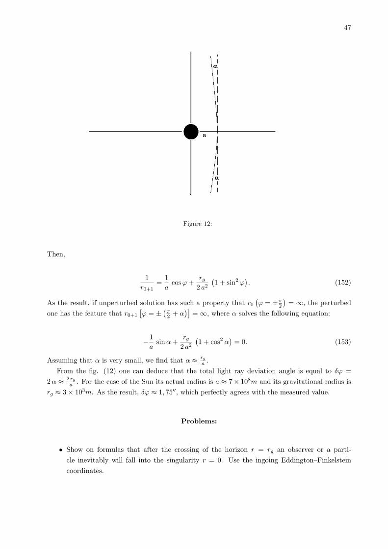
47

Figure 12:

Then,

1r0+1

=1a

cosϕ+rg

2 a2

(1 + sin2 ϕ

). (152)

As the result, if unperturbed solution has such a property that r0(ϕ = ±π

2

)= ∞, the perturbed

one has the feature that r0+1

[ϕ = ±

(π2 + α

)]=∞, where α solves the following equation:

−1a

sinα+rg

2 a2

(1 + cos2 α

)= 0. (153)

Assuming that α is very small, we find that α ≈ rga .

From the fig. (12) one can deduce that the total light ray deviation angle is equal to δϕ =2α ≈ 2 rg

a . For the case of the Sun its actual radius is a ≈ 7× 108m and its gravitational radius isrg ≈ 3× 103m. As the result, δϕ ≈ 1, 75′′, which perfectly agrees with the measured value.

Problems:

• Show on formulas that after the crossing of the horizon r = rg an observer or a parti-cle inevitably will fall into the singularity r = 0. Use the ingoing Eddington–Finkelsteincoordinates.

48

• Show that in the Schwarzschild metric there are circular light like orbits at r = 3rg/2.


• Pound–Rebka experiment and other classic experiments in General Relativity.

• How does Global Positioning System or Glonass system works? (“Relativity in the GlobalPositioning System”, Neil Ashbey, Living Reviews in Relativity, 6 (2003) 1.)

• Particle orbits and absorbtion cross–sections for black holes.

49

LECTURE VIIEnergy–momentum tensor for a perfect relativistic fluid. Interior solution. Kerr’s rotating black

hole. Concise comments on Cosmic Censorship Hypothesis and on the No Hair Theorem.

1. In this lecture we find a solution of Einstein equations which describes a stable star — anideal ball of matter surrounded by vacuum. This is referred to as interior solution. Inside the ballwe assume that the energy–momentum tensor is not zero, Tµν 6= 0, but it is homogeneous andspherically symmetric. At the same time outside the ball there is vacuum, i.e. Tµν = 0 and Λ = 0.

To have a stable star, inside it there should be a matter, which is capable to create a strongenough pressure to prevent its collapse. Hence, Tµν of a dust, which was considered in the previouslectures, is not sufficient. The appropriate energy momentum tensor is given by

Tµν(x) = ρ(x)uµ(x)uν(x) + p(x)[uµ(x) uν(x)− gµν(x)

], (154)

where gµν is the metric tensor and x = (t, ~x) is the coordinate four–vector. We start with providingarguments that this is the energy momentum tensor for a relativistic perfect fluid and ρ is theenergy density, while p is the pressure. In fact, in the reference system, where the fluid is static its

four–velocity is uµ =(g− 1

200 , 0, 0, 0

)and then

||Tµν || = Diag (ρ,−p,−p,−p) , Tµν = gµα Tαν . (155)

Already this form of the tensor can reveal the physical meaning of ρ and p, as follows from thecourse of classical electrodynamics.

Furthermore, the condition of the conservation of this energy momentum tensor is as follows:

0 = Dµ Tµν = (ρ+ p) uµDµuν +Dµ [(ρ+ p)uµ] uν −Dνp. (156)

Multiplying this equality by uν and using that uν uν = 1 (and, hence, uν Dµuν = 0), we arrive atthe following equation:

Dµ [(ρ+ p) uµ]− uµDµp = Dµ [ρ uµ] + pDµ uµ = 0. (157)

The last equality is just a covariant generalization of the continuity equation in the flat space–time:∂µ [ρ uµ] = ρ+ div [ρ~v] = 0. Note that in the non–relativistic limit the pressure is always much lessthan the energy density, p ρ, for the same reason as why non–relativistic kinetic energy is muchsmaller than the rest energy.

Using (156) and (157), we find the following equation:

(ρ+ p) uµDµuν = (δαν − uα uν) Dαp, (158)

50

Here ||δαν − uα uν || = Diag(0, 1, 1, 1) — is the projector on spatial directions. Hence, this is arelativistic, covariant extension of the Euler equation for a liquid without viscosity:

ρ[∂t~v +

(~v, ~∇

)~v]

= −~∇p. (159)

The last equation is just the Newton’s second law, m~a = ~F , both sides of which are attributed perunit volume. In fact,

~a [t, ~x(t)] ≡ d~v [t, ~x(t)]dt

= ∂t~v + (∂i~v) (∂txi) = ∂t~v +(~v, ~∇

)~v,

and recall that the pressure p is just a force attributed per unit area. The Euler equation can berewritten in the following form:

∂t (ρvi) + ∂j Tij = 0 (160)

with the use of the tensor Tij = ρ vi vj + p δij .All in all, the given above arguments should convince the reader that (154) is the energy

momentum tensor for a relativistic perfect fluid. To specify the fluid one just has to choose anequation of state — p = p(ρ), i.e. the relation between the pressure and density of the fluid.

2. Thus, we are looking for a time–independent, spherically symmetric and regular everywheresolution of the Einstein equations with the energy–momentum tensor, which is given by (154) withρ = ρ(r) and p = p(r) for r ≤ R, and ρ = 0 = p for r > R. Then the appropriate ansatz for themetric should be as in the lecture IV:

ds2 = eν(r) dt2 − eλ(r) dr2 − r2 dΩ2, (161)

where ν and λ are functions of r only, because we are looking for static and spherically symmetricsolution. For such a metric we obtain the Einstein equations that are following from those foundin the lecture IV:

8π κ ρ(r) = R00 −

12R =

e−λ

rλ′ +

1r2

(1− e−λ

),

−8π κ p(r) = R11 −

12R = −e

−λ

rν ′ +

1r2

(1− e−λ

),

−8π κ p(r) = R22 −

12R = −e

− ν+λ2

2

[d

dreν−λ

2

]− e−λ

2 rν ′ +

e−λ

2 rλ′. (162)

Here ν ′ ≡ dν/dr and λ′ ≡ dλ/dr. The rest of the components of the Einstein equations eitherfollow from (162) or lead to the trivial relations, stating that 0 = 0.

The first equation in (162) contains only λ and can be rewritten as:

51

1r2

d

dr

[r(1− e−λ

)]= 8π κ ρ(r). (163)

Its solution is as follows:

e−λ(r) = 1− 2κM(r)r

, where

M(r) = 4π∫ r

0dxx2 ρ(x) + c, (164)

and c is an integration constant. To obtain a solution, which is regular at r = 0, we have tochoose c = 0. Also to avoid having a horizon — a surface, beyond which coordinate r ceases tobe space–like and becomes time–like — we have to have that everywhere e−λ(r) > 0. Hence, thereshould be r ≥ 2κM(r), which imposes a restriction on the density ρ(r).

As we have assumed above ρ(r) = 0, if r > R. In this region we expect that the solution(161) acquires the form of the Schwarzschild one. And indeed it does that with the mass equal toM ≡M(R) = 4π

∫ R0 dr r2 ρ(r). But the real mass of the star should be

Mreal =∫Bd3V

√g(3) ρ(r) =

∫ R

0dr

∫ π

0dθ

∫ 2π

0dϕ sin θ r2 eλ/2 ρ(r) = 4π

∫ R

0

dr r2 ρ(r)√1− 2κM(r)

r

,

where B is the body of the star, d3V√g(3) is the volume form of the three–dimensional time–slice,

following from the metric (161). Correspondingly g(3) is the determinant of the three–dimensionalspatial part of the metric (161). Thus, the difference Ebin = Mreal −M > 0 is the gravitationalbinding energy.

Coming back to (162), from the second equation we find that

dν

dr=

2κM(r) + 8π r3 κ pr [r − 2κM(r)]

. (165)

In the Newtonian limit, p ρ and κM(r) r, this equation reduces to dν/dr ≈ 2κM(r)/r2,i.e. to the spherically symmetric version of the Poisson equation for the gravitational potential.Thus, in the case of the static, spherically symmetric gravitational field, ν/2 has the meaning ofthe relativistic analog of the Newtonian potential.

Instead of the last equation in (162) it is convenient to use the condition of the conservation ofthe energy–momentum tensor, Dµ Tµν = 0. In our case it reduces to the following equation:

2dp

dr= − (p+ ρ)

dν

dr. (166)

Hence, using eq. (165) here, we obtain:

dp

dr= − (p+ ρ)

κM(r) + 4π r3 κ pr [r − 2κM(r)]

, (167)

52

which is the so called Tolman–Oppenheimer–Volkoff equation for the hydrodynamic equilibrium ofthe star. In the Newtonian limit, p ρ and κM(r) r, this equation reduces to:

dp

dr≈ −ρ κM(r)

r2. (168)

3. In conclusion, we have found that the metric for a homogeneous, static, spherically symmetricand non–rotating star is as follows:

ds2 = eν(r) dt2 − dr2

1− 2κM(r)r

− r2 dΩ2, (169)

where M(r) is defined in (164), while ν(r) follows from (165). At the same time, the necessaryand sufficient condition of the star equilibrium is given by the equation (167).

Outside the star body p = 0 and ρ = 0, hence, one can solve (165) to find that eν = 1− 2κM(R)r .

As the result outside the star surface, r ≥ R, the solution under consideration reduces to theSchwarzschild one.

To solve the equations (164), (165) and (167) explicitly one has to specify the equation of statep = p(ρ). The simplest model corresponds to the incompressible fluid, when ρ = ρ0 = const. ThenM(r) = 4π

3 r3 ρ0 for r < R and the solution of (167) is as follows:

p(r) = ρ0

√1− 2κM

R −√

1− 2κM r2

R3√1− 2κM r2

R3 − 3√

1− 2κMR

, M =4π3R3 ρ0. (170)

From this equation it is not hard to see that the central pressure p(r = 0) blows up to infinity ifR = 9

4 κM . That simply means that stars with M > Mmax = 49κ R cannot exist, if their matter

consists of the incompressible fluid.4. To draw the corresponding Penrose–Carter diagram it is convenient to choose the relevant

(t, r) part of the space–time and to make the following coordinate change:

eν(r) dt2 − dr2

1− 2κM(r)r

= eν(r)

dt2 − dr2

eν(r)[1− 2κM(r)

r

] = eν(r)

[dt2 − dr2∗

],

where dr2∗ ≡dr2

eν(r)[1− 2κM(r)

r

] . (171)

Here r∗ is ranging from 0 to +∞, unlike tortoise r∗, which is ranging from −∞ to +∞. That isbecause the denominator in the definition of dr∗ does not have a pole for any r, due to the regularityof the solution under consideration. The range of values of r∗ can be adjusted to [0,+∞) by asuitable choice of the integration constant in the relation between r∗ and r.

As the result, if we make the same transformation for t ± r∗ as the one which was done atthe beginning of the lecture V, we arrive at the diagram shown on the fig. (13). The grey region

53

Figure 13:

on this picture shows the star’s body. The resulting picture is just a half of the MinkowskianPenrose–Carter diagram, which was shown at the beginning of the lecture V. It is similar to thediagram of the (t, r) part of the Minkowski space–time in the spherical coordinates.

5. We continue our consideration of collapse and star solutions with the concise discussionof the most general stationary, vacuum solution of the Einstein equations. This is the so calledKerr’s rotating black hole. With the use of the so called Boyer–Lindquist coordinates its metriccan be represented in the following form:

ds2 =∆− a2 sin2 θ

ρ2dt2 +

4κM a

ρ2r sin2 θ dϕ dt− ρ2

∆dr2 − ρ2 dθ2 − A sin2 θ

ρ2dϕ2,

where ∆ = r2 − 2κM r + a2,

ρ2 = r2 + a2 cos2 θ,

A =(r2 + a2

)2 − a2 ∆ sin2 θ. (172)

This metric is stationary but not static. In fact, components of the metric tensor are time inde-pendent. However, the line element (172) is not invariant under time inversion t→ −t, due to thepresence of the non–diagonal term dt dϕ.

While Schwarzschild black hole depends on one parameter M , the Kerr solution depends ontwo parameters M and a. It reduces to the Schwarzschild black hole if a = 0. In the asymptoticspatial infinity, r →∞, Kerr’s metric simplifies to:

54

Figure 14:

ds2 ≈(

1− 2κMr

)dt2 +

4κM a sin2 θ

rdt dϕ−

(1 +

2κMr

)dr2 − r2dΩ2. (173)

This is the week gravitational field, which describes massive rotating body with the angular mo-mentum J = M a, which explains the physical meaning of the parameter a. (See the correspondingparagraph of Landau–Lifshitz for more details.)

It is not hard to notice that g11 component of metric is singular when ∆ = 0. The corresponding

quadratic equation has two solutions r± = κM ±√

(κM)2 − a2. As a → 0 one can find thatr+ → rg, while r− → 0. This is the hint that r+ is the event horizon. Explicitly this fact canbe seen, e.g., from the corresponding Penrose–Carter diagram, drawing of which goes beyond thescope of our lectures. Another option is to see that the normal vector to the surface r = r+ islight–like, which is left as an exercise for the reader.

Furthermore, the condition g00 = 0 has two solutions. The outer one, r0(θ) = κM +√(κM)2 − a2 cos2 θ, defines the boundary of the so called ergoregion. As the result one en-

counters the picture shown on the fig. (14): the event horizon is surrounded by the ergoregion. Ifan observer finds himself inside the ergoregion, he in principle can escape to spatial infinity. Thiscan be seen, e.g., from the corresponding Penrose–Carter diagram or from the fact that the normalvector to the ergosphere r0(θ) is not light–like.

6. Now it is worth pointing out that equations ∆ = 0 and g00 = 0 have real solutions only ifκM > a. Otherwise the singularity of the space–time under consideration is not hidden behind theevent horizon. In the latter case the singularity will be reachable within finite time as measured by

55

any distant observer. Moreover, it can be shown that in this case there are closed time–like curves.Such a peculiar situation seems to be physically unacceptable. As the result scientific communitybelieves in the so called Cosmic censorship hypothesis.

Vague formulation of this hypothesis is as follows. Einstein equations can have many spurious(unphysical) solutions, e.g., having naked singularities (not surrounded by event horizons) or closedtime–like loops. But physicists believe that in real situations black holes are results of collapseprocesses. Hence, it is natural to expect that during these processes any physically measurablequantity remains regular. The question is, however, whether one can achieve this within the theoryof General Relativity or one has to modify it? In any case we expect that singularities cannot becreated and, e.g., the Kerr solution is physically meaningful only if κM ≥ a. The solution withκM = a is referred to as critical.

Another important property of black holes is provided by the so called No Hair Theorem. Theproof of this theorem goes beyond the scope of our lectures, but in simple terms it can be explainedas follows. It states that the final stage of a generic collapse process is given by a stationary Kerrsolution, if the total electric charge of the black hole is zero.

The point is that black hole horizon, as we have explained in the previous lectures, is a surface ofthe infinite redshift — from any frequency to its zero value. Namely, if someone creates a radiationjust behind the horizon, it cannot be seen even just outside the horizon. In fact, whatever happensbehind the horizon, observers outside it, resting at any radius, still see only stationary fields dueto the infinite redshift.

This observation, probably, will help to acquire an intuitive understanding of the followingpicture. Obviously during a collapse process, if there is no any spherical symmetry, there are plentyof radiation processes. However, as the matter of the collapsing star, the source of the radiationunder discussion, approaches the corresponding Schwarzschild radius, this radiation experiencehigher and higher redshift. As the result independently of the frequency of the initial radiation,which was created in the vicinity of the horizon surface, distant observers see fields which are closerand closer to the stationary ones, as the collapse process is approaching its termination. Such asituation reveals itself via the following effect: All intensities for multi–pole radiations are fallingas inverse powers of time.

All in all, during the collapse process, everything which can be radiated is indeed radiated awayand the outside observes eventually detect only stationary fields. As we will see in the lecturesIX and X, to have a gravitational radiation there should be at least quadruple moment changingin time (or higher momenta). Also it is known that to have an electromagnetic radiation thereshould be at least dipole moment changing in time. Thus, monopole electric moment (i.e. electriccharge), monopole gravitational moment (i.e. mass) and dipole gravitational moment (i.e. angularmomentum) are capable to provide only stationary fields. It is this content that can remain for thegravitational and electromagnetic fields at the end of the collapse process. As the result, the mostgeneric black hole, in the presence of the electromagnetic fields, can carry only three parameters— mass, angular momentum and electric charge. Note that to create a radiation of scalar fieldsit is sufficient to have a monopole moment (i.e. the corresponding charge) changing in time. Asthe result black holes cannot carry “scalar hairs”. This completes the intuitive explanation of the

56

essence of the No Hair theorem.

Problems:

• Show that for the Kerr solution the normal vector to the surface r = r+ is light–like. (Seethe corresponding paragraph in Landau–Lifshitz.)

• Show that one can escape from the ergoregion.


• Criteria for the star stability. Chandrasekhar limit. (Stars and relativity, Y.B. Zel’dovichand I.D. Novikov, University of Chicago Press, 1971)

• Penrose–Carter diagram for Kerr solution.

• No Hair Theorem.

• Cosmic censorship hypothesis.

• Membrane paradigm. Black hole horizon as a viscous liquid having electric conductivity.Black hole thermodynamics

• Zeldovich–Penrose effect. Energy extraction from the ergoregion.

• Multi–pole radiation during the collapse process. (“Nonspherical perturbations of relativisticgravitational collapse. I. Scalar and gravitational perturbations”, R.H. Price, Phys. Rev. D5 (1972) 2419)

57

LECTURE VIIIOppenheimer–Snyder collapse. Concise comments on the origin of the thermal nature of the

Hawking’s radiation and on black hole creation.

1. In this lecture we continue the discussion of the physics underlying the Schwarzschild geome-try. Namely we find here the so called Oppenheimer–Snyder solution, which describes the collapseprocess of a spherically symmetric, non–rotating body into the black hole.

Consider a static star (a ball filled with a matter) surrounded by empty space. The star is staticdue to an internal pressure until some moment of time t = 0 and then the pressure is switched off.Say before t = 0 there were some thermonuclear processes inside this star, which were producingthe internal pressure. But by the moment t = 0 the entire thermonuclear fuel was used out.

To model the collapse process after t = 0 we assume that inside the star there is a homogeneouspressureless dust. Also we assume that the original star was ideal ball with ideal spherical surfaceand that the collapse process goes in such a way that homogeneity of the matter inside the starand the spherical symmetry is never violated. This is a highly unstable situation because any itsperturbation violating these symmetries will grow in time due to the tidal forces. We neglect suchperturbations.

Thus, inside the ball the energy momentum tensor is Tµν = ρ(τ)uµuν , where the density ρ(τ)is just a function of time τ because of the spatial homogeneity. Outside the ball we have vacuum,Tµν = 0.

Such a massive ball of matter should create a spherically symmetric and asymptotically flatgravitational field in vacuum. Thus, due to Birkhoff theorem outside the ball the metric has tobe the Schwarzschild one. Any violation of the spherical symmetry will lead to time–dependentgravitational fields in vacuum, i.e. to a creation of gravitational waves, which are discussed in thelectures IX and X. Neglecting such processes is exactly the approximation that we use here.

To give an intuitive explanation why spherically symmetric collapse does not create gravitationalradiation, let us discuss the following situation. Consider a ball which is electrically charged andthe charge is homogeneously distributed over its volume. Suppose now that for some reason thisball rapidly shrinks in such a way that the homogeneity and spherical symmetry are respected. Itis not hard to see that independently of the radius of the ball it creates the same Coulomb fieldoutside itself. This is related to the uniqueness of the Coulomb solution of the Maxwell equations,which was mentioned in the lecture IV.

Thus, the magnetic field outside the ball is vanishing and such an accelerated motion of thecharge does not create an electromagnetic radiation. The point is that to have a radiation thereshould be at least dipole moment, which is changing in time, while in the case of the ball allmomenta are zero with respect to its center. It happens that to have a gravitational radiation,as we will see in the lectures IX and X, there should be even quadruple moment, which changesin time. Dipole moment changing in time is not enough for the generation of the gravitationalradiation. Also from the Newton’s gravitation we know that an ideal spherical massive ball createsthe same potential outside itself independently of its radius. The form of the potential just depends

58

on the mass of the ball. In general relativity the situation is similar due to the Birkhoff’s theorem.2. All in all, the metric outside the ball is

ds2+ =(1− rg

r

)dt2 − dr2

1− rgr

− r2 dΩ2. (174)

Here rg = 2κM , where M is the mass of the ball, which remains constant during the collapseprocess, because of the absence of the radiation. Intuitively it should be clear that then there is noenergy which fluxes away to infinity with the radiation and the energy of the ball remains constant.

This metric is valid outside of the surface of the ball Σ, which radially shrinks down duringthe collapse process. Then the world–hypersurface of Σ is zµ(τ) = [T (τ), R(τ)] and at every giventime slice it is an ideal sphere. (Note that in this lecture we denote by the same Σ both thethree–dimensional world–hypersurface and its two–dimensional time–slices.) Hence, Σ occupies allthe values of the spherical angles θ and ϕ. Here R(τ) decreases as the proper time τ goes by. Theinitial value of the R(τ0) = R0 is grater than rg. Otherwise at the initial stage we would have hada black hole rather than a star.

Inside the ball we have a spatially homogeneous metric whose time–slices are compact and aredecreasing in size as time goes by. The suitable metric is:

ds2− = dτ2 − a2(τ)[dχ2 + sin2 χdΩ2

], dΩ2 = dθ2 + sin2 θ dϕ2. (175)

We discuss the physics and the origin of such metrics in the lecture XI in grater details. Its spatialsection dτ = 0 is the three–sphere, whose metric is a2(τ)

[dχ2 + sin2 χdΩ2

], χ ∈ [0, π]. The radius

of the three–sphere a(τ) is decreasing as the time τ goes by.Thus, we have

gττ = 1, gχχ = −a2, gθθ = −a2 sin2 χ, and gϕϕ = −a2 sin2 χ sin2 θ. (176)

The resulting non–zero components of the Christoffel symbols are Γ0ij = a agij and Γi0j = a

a δij .

Here a ≡ da/dτ , i = 1, 2, 3 and gij is the metric of the three–sphere of unit radius. As the resultΓijk components of the Christophel symbols also are not zero and are proportional to those of thethree–sphere, but we do not need their explicit form in this lecture.

One can find from these Christoffel symbols that the “00” part of the Einstein tensor, Gµν ≡Rµν − 1

2 gµν R, has the following form:

G00 =3a2

(a2 + 1

). (177)

At the same time the energy–momentum tensor inside the ball is Tµν = ρ(τ)uµ uν . In the referenceframe of (175) the dust remains stationary, i.e. dχ = dθ = dϕ = 0. Hence, uµ = (1, 0, 0, 0) and theonly non–zero component of Tµν is T00 = ρ(τ). As the result from (177) we find that one of theEinstein equations is as follows:

59

a2 + 1 =8πκ3

ρ a2. (178)

Equations for T0j do not lead to non–trivial relations: they just give relations stating that 0 = 0.As we have explained at the end of the lecture III, instead of some of the remaining equations onecan use the energy–momentum tensor conservation condition,

0 = DµTµν = ∂µ (ρ uµ uν) + Γµβµ ρ u

β uν − Γβνµ ρ uµ uβ . (179)

Here we have four equations — one for each value of ν. If ν = 1, 2, 3 then again we get trivialrelations 0 = 0. However, if ν = 0 there is the following equation:

ρ+ 3a

aρ = 0, where ρ =

dρ

dτ. (180)

Hence, ∂τ(ρ a3

)= 0 and we obtain the obvious result that if the volume of spatial sections decreases

as a3(τ) the density of the dust is increasing as ρ(τ) = consta3(τ)

. Let us choose here such a constantthat ρ a3 = 3

8πκ a0. Then the solution of (178) has the following parameterized form:

a(η) =a0

2(1 + cos η) , and τ(η) =

a0

2(η + sin η) . (181)

We discuss the physical meaning of the parameter η and of such solutions in the lecture XI in graterdetails. Here we just check that (181) indeed solves (178). In fact, dτ

dη = a02 (1 + cos η) = a(η).

Then, dadτ = da

dηdηdτ = da

dη1a . As the result from (178) we derive the simple oscillator equation

(da

dη

)2

+ a2 = a0 a. (182)

Obviously a(η) from (181) solves this equation. The integration constants in (181) are chosen tofulfill the initial conditions.

From (181) we see that the collapse starts at η = 0, which corresponds to τ = 0. In Schwarzschildcoordinates this corresponds to t = 0, when the thermonuclear fuel inside the ball was completelyspent. At this moment a = a0. The collapse ends as a → 0. That happens as η → π, i.e. whenthe proper time reaches τ = πa0

2 . Thus, the collapse process takes the finite proper time: the shellcrosses the horizon r = rg and even reaches the singularity within the finite proper time.

3. What remains to be done is to glue the metrics ds2+ and ds2− and their first derivatives acrossthe surface Σ of the ball. Their second derivatives, which are related to the Ricci tensor, are fixedby Einstein equations.

In terms of the metric ds2− the surface Σ is just a two sphere at some value χ0 of the angle χ.Then the induced metric on the surface is

ds2−∣∣Σ

= dτ2 − a2(τ) sin2 χ0 dΩ2. (183)

60

This metric has to be related to the one on the world–hypersurface zµ(τ) = [T (τ), R(τ)] in theSchwarzschild background:

ds2+∣∣Σ

=

[(1− rg

R

) (dTdτ

)2

− 11− rg

R

(dR

dτ

)2]dτ2 −R2(τ) dΩ2. (184)

To have that ds2−∣∣Σ

= ds2+∣∣Σ, there should be relations as follows:

R(τ) = a(τ) sinχ0,(1− rg

R

) (dTdτ

)2

− 11− rg

R

(dR

dτ

)2

= 1. (185)

These relations allow us to find R(τ) from (181) and, then, T (τ) from the equation:

T =

√R2 + 1− rg

R

1− rgR

, where T =dT

dτ, and R =

dR

dτ. (186)

This is the world–hypersurface of the boundary of the ball as it is seen by outside observers.From the last equation one can see that as R→ rg in the collapse process, we can neglect 1− rg

R

in comparison with R2 under the square root. Then,

dT ≈ − dR

1− rgR

, (187)

and the minus sign appears here because during the collapse process we have that dR < 0, whiledT > 0. Thus, one obtains that

R(T ) ≈ rg(

1 + e− Trg

), (188)

i.e. from the point of view of an observer, which is fixed at some r > R(τ), the fall of the star’smatter through the surface r = rg never happens. The matter of the star just asymptoticallyapproaches its gravitational radius as t → +∞. That is true although the star falls behind itsgravitational radius within the above mentioned finite proper time.

The next step is to glue the first derivatives of ds2− and ds2+ across Σ. This demands somestraightforward calculations with the use of differential geometry for surfaces in curved space–times. This goes beyond the scope of our lectures. But the result of the calculation is very simpleand can be predicted on general physical grounds. In fact, from the gluing conditions in questionone finds that

rg = 2κ4π3ρ(τ)R3(τ) = const. (189)

61

Figure 15:

Which just means that the mass of the star/black hole remains constant during the ideal spher-ical collapse. Moreover, the mass is appropriately related to the gravitational radius, rg, of theSchwarzschild geometry.

4. Let us draw the Penrose–Carter diagram for the Oppenheimer–Snyder collapsing solution.To do that we have to draw separately the diagrams for ds2+ and ds2− and to glue them across Σ.For the Schwarzschild part, ds2+, the diagram follows from the fig. (15). This is just the samediagram as in the last lecture, but it is valid only beyond Σ whose world–surface is [T (τ), R(τ)]after t = 0. Before t = 0 the surface Σ remains stationary at some radius r = R0 > rg.

To draw the Penrose–Carter diagram for ds2− let us represent this metric as follows:

ds2− = dτ2 − a2(τ)[dχ2 + sin2 χdΩ2

]= a2(η)

[dη2 − dχ2 − sin2 χdΩ2

], (190)

where η ∈ [0, π] is defined in (181). Now we should drop off the conformal factor a2(η) andchoose the relevant two–dimensional part i.e. (η, χ). Then we obtain just a part of the square for0 ≤ χ ≤ χ0 and 0 ≤ η ≤ π. This has to be glued to the diagram for the fig. (15) after t = 0.Before this moment of time the Penrose–Carter diagram of the space–time behind Σ is the sameas was found in the previous lecture.

All in all, this way one finds the total Penrose–Carter diagram for the Oppenheimer–Snydercollapsing solution which is shown on the fig. (16). It can be adjusted to the shown here form bya suitable conformal transformation. It is worth stressing at this point that in doing this gluing ofdiagrams we drop off different conformal factors for different parts of the diagram.

62

r = 0

r = rg

t = 0

Σ

Figure 16:

As one can see, the obtained diagram does not contain the white hole part. But it is not hardto find the time reversal of the collapsing solution. It is given by the same equation as (181) forη ∈ [π, 2π] or by

a(η) =a0

2(1− cos η) , and τ(η) =

a0

2(η − sin η) , (191)

if one chooses η ∈ [0, π]. This solution describes explosion starting from η = 0, when τ = 0and a = 0. Then as η reaches π the conformal factor inflates to a = a0. If something stops theexplosion at a = a0, then the corresponding Penrose–Carter diagram is just the time reversal ofthe one shown on the fig. (16), i.e. it is the flip of this picture over a horizontal line.

5. We continue this lecture with the discussion of two complicated, but very important ques-tions. Let us see now what happens with waves which are created in the vicinity of a black holehorizon. The arguments, which are presented here, are borrowed from the book “General Relativ-ity” by I. Khriplovich. Consider say an electromagnetic excitation, which is created at a radiusr0 = rg + ε, ε rg in the vicinity of the horizon. Radial propagation time of this excitation fromr0 to r rg follows from the equation:

0 = ds2 =(1− rg

r

)dt2 − dr2

1− rgr

, (192)

and is equal to

t =∫ r

r0

dr

1− rgr

= r − r0 + rg logr − rgr0 − rg

≈ r + rg logr

ε. (193)

63

If the frequency of the excitation at r0 is equal to ω0, then, as follows from the fact that ω√g00(r)

is a conserved quantity according to the time–like killing vector, at r r0 the frequency is reducedto

ω = ω0

√g00(r0)g00(r)

≈ ω0

√ε

rg. (194)

This effect can be understood on general physical grounds. In fact, a photon performs a work toclimb out from the gravitational attraction of the massive center. Then its energy and, hence,frequency should reduce.

As follows from (193),

ε

r≈ e−

t−rrg . (195)

Hence, the frequency of the excitation, as it crawls out from the vicinity of the horizon, dependson time as follows:

ω(t) ≈ ω0

√r

rge− t−r

2rg . (196)

Furthermore, the phase of the electromagnetic excitation is changing as

Ψ(t) =∫ t

0dt′ω(t′) ≈ −2ω0

√r rg e

− t−r2 rg + const. (197)

This way we have found eikonal Ψ, i.e. eiΨ is the solution of the Maxwell equations in the geometricoptic approximation and with the given above initial conditions. Then the spectrum of frequenciescontributing to this wave–packet is as follows:

f(ω) ∼∫ ∞

0dt ei ω t exp

[−2 i ω0

√r rg e

− t−r2 rg

]∼(2ω0√r rg)2 i ω rg e−π ω rg Γ (−2 i ω rg) , (198)

where Γ(x) is the Γ–function. Here we have dropped off the factors that do not depend on ω. Asthe result, the spectral density of any wave–like excitation that was created in the vicinity of thehorizon is given by:

|f(ω)|2 ∼ e−2π ω rg |Γ (−2 i ω rg)|2 =π

ω rg

1e4π ω rg − 1

≈ π

ω rge−4π ω rg . (199)

The last approximation is used because our estimates are valid in the geometric optic approxima-tion, when ωrg 1.

This calculation is absolutely classical. However, if in the last expression we multiply ω by ~,to obtain the energy, E = ~ω, then the exponent will acquire the form of the Boltzman’s thermalfactor:

64

w(E) ∼ e−ET , (200)

where T = ~4π rg

is the so called Hawking’s temperature. Hawking effect is that black holes aredecaying via creation of particles with the thermal spectrum. Formally, Hawking radiation of blackholes follows from similar equations. However, conceptually the effect in question is much morecomplicated and its discussion goes beyond the scope of our lectures. To stress the difference let usjust point out here that Hawking effect follows from a change of the ground state of quantum fieldsdue to a collapse process and does not have a source so to say. At the same time, in this sectionwe just have made an observation that if there is a radiation, which is sourced in the vicinity ofthe horizon, it will thermalize as it climbs out to infinity.

6. Another seemingly unrelated question is as follows. Does actually the creation of the blackhole ever happens from the point of view of those who always stay outside it? Or do they just seesuch an eternal asymptotically slowing down process which was described above? Although thisis just an academic question, because there seems to be no device which will be always sensitiveto the exponentially suppressed factor e−t/rg in (188) or in (196), as t → +∞, we still would liketo address it here. We think that the answer to this question may be relevant for the deeperunderstanding of the Hawking radiation and backreaction on it. Note that, as pointed out above,formally this effect appears due to the same exponential factor.

Now we present some intuitive speculations, which still need to get some solid mathematicalapproval. Let us see what happens with the light rays which are scattered off the surface of thestar or radiated by it. If one has absolutely sensitive device and takes the above picture seriously,he is expecting to see that the signal will be eternally coming out from the star.

However, this picture is valid only if we assume that light rays are going along light–like geodesicson the Schwarzschild background. That is true, if one neglects that an electromagnetic wave itselfcarries energy and, hence, also curves space–time. The latter effect is very small, but the questionis if one can neglect it, once he addresses the issues of the exponentially suppressed contributions.

To understand what we are actually up to here, consider the fig. (5) of the lecture IV. Fromthe corresponding picture one can see that the horizon is just one of the light–like geodesics. It isa boundary between two families of “outgoing” geodesics. Moreover if a light ray was going alongthe horizon it will remain there eternally.

However, if one takes into account that electromagnetic field also does curve space–time, hehas to draw real light–like world–lines rather than geodesics. The picture of the fig. (5) fromthe lecture IV is not applicable anymore. Apart from all the new picture will not be static. Butcertain its relevant features will remain unchanged. Namely, we still expect to have two familiesof “outgoing” light–like world–lines — those which escape to infinity and those which are directedtowards the singularity. To see this one can just study short parts of the world–lines in question,i.e. seeds of light–like lines during small periods of time. But the boundary separating these twofamilies of curves will not belong to the class of the light–like world–lines. The light ray cannotanymore eternally stay on the fixed radius r = rg.

Rephrasing this, we expect that among the photons, which are emitted by a collapsing star,

65

there will be a last one that will reach outside observers. The next photon after that will justparticipate into the creation of the black hole as a part of its matter content. As the result, theoutside observer sooner or latter will stop receiving signals sourced by the matter of the collapsingstar. And that will happen objectively rather than due to a lack of the sensitivity of his device.

One of the disadvantages of the picture that we have described here is that, if it is true, thenthe moment of black hole formation depends on the energy of the last escaping photon. But atthis point for us it is important to see that the black hole is actually created during a finite timeas measured by outside observers. In any case we just qualitatively described some phenomenonwhich remains to be described quantitatively somehow.

Problems

• Calculate the Christoffel symbols and the Ricci tensor for the metric ds2−.


• Thin–shell collapse and Vaidya space–time.

• Gluing conditions for metric tensors, extrinsic curvature and differential geometry of embed-ded hypersurfaces.

• Derivation of the Hawking radiation (see e.g. “Hawking radiation and secularly growingloop corrections”, Emil T. Akhmedov, Hadi Godazgar and Fedor K. Popov; Published inPhys.Rev. D93 (2016) 2, 024029; e-Print: arXiv:1508.07500)

• Black hole thermodynamics.

• Eikonal, geometric optic or quasiclassical approximation for wave equations. Hamiltonian–Jacoby equations in various situations.

66

LECTURE IXEnergy–momentum pseudo–tensor for gravity. Weak field approximation. Energy–momentum

pseudo–tensor in the weak field limit on the Minkowskian background. Free gravitational waves.

1. To define what means gravitational radiation one has to specify the meaning of energy fluxin the presence of gravity. That is the problem we are going to address in this lecture.

In Minkowski space–time the energy–momentum conservation has the following form ∂µTµν = 0.After the integration over a time–slice Σ and application of the Stokes theorem, this equationexpresses the actual conservation of a quantity referred to as four momentum:

dP 0

dt+∮∂Σd2σi Ti0 = 0, where Pµ(t) ≡

∫ΣTµ0 (t, ~x) d3Σ(~x) . (201)

Here d3Σ(~x) is the volume element of a Cauchy surface, Σ, or of a time–slice t = const; t is timeand d2σi is the area element of the boundary ∂Σ of the Cauchy surface in question. Having sucha quantity, one can define what means energy inflow or outflow,

∮∂Σ d

2σi Ti0, in a system. In thepresence of gravity, however, the equation, that we have been referring to as energy–momentumconservation law in the previous lectures, has the form as follows — DµTµν = 0. It can betransformed into:

0 = DµTµν = ∂µT

µν + Γµβµ T

βν − Γβνµ T

µβ =

1√|g|

∂µ

(Tµν√|g|)− 1

2(∂νgµα) Tµα, (202)

where we have used that Tµν = T νµ and the expression Γµνµ = 1√|g|∂ν√|g|, which follows from the

definition of the Christoffel symbols.Unlike the equation ∂µTµν = 0 the obtained relation (202) does not express any actual conser-

vation of some quantity. This is natural to expect in the presence of gravity, because the energyand momentum carried only by matter, Tµν , should not be conserved alone. In fact, there can beenergy–momentum transfer between matter and gravity. But then what is a quantity that describesenergy–momentum for gravity itself? What is the total energy–momentum tensor for gravity andmatter together, which we expect to be conserving?

Let us choose such a reference system at a point x0 that ∂αgµν(x0) = 0. (Note that this choiceof the frame does not mean that gµν(x0) = ηµν .) From (202) we obtain that ∂µT

µν (x0) = 0, because

in such a reference frame also ∂µ√|g(x0)| = 0. How does this equation change in an arbitrary

gauge, i.e. in an arbitrary reference system?From the Einstein equations of motion it follows that Tµν = 1

8π κ

(Rµν − 1

2 gµν R

). At the same

time in the above defined gauge we have that Γµνα(x0) = 0, but ∂βΓµνα(x0) 6= 0 and, hence, from

the definition of the Ricci tensor we have that

Rµν(x0) =12gµα gνγ gσδ [∂α∂δgσγ + ∂σ∂γgαδ − ∂α∂γgσδ − ∂σ∂δgαγ ] . (203)

67

Plaguing this expression into the Einstein equations and performing straightforward transforma-tions, we obtain that:

Tµν(x0) = ∂α

1

16π κ1|g|

∂β

[|g|(gµν gαβ − gµα gνβ

)]≡ 1|g|

∂αηµνα, (204)

in the reference frame under consideration. Here

ηµνα =1

16π κ∂β


)]. (205)

In eq.(204) we have used that ∂α |g(x0)| = 0 and took |g| out from the derivative ∂α. This quantityhas obvious properties, which follow from its definition:

ηνµα = ηµνα = −ηµαν . (206)

Thus, in the gauge ∂αgµν(x0) = 0 we have the following relation: ∂αηµνα(x0) = |g|Tµν(x0). In anarbitrary gauge this relation is not true. Hence, let us define

∂αηµνα − |g|Tµν ≡ |g| tµν . (207)

The newly defined quantity tµν is symmetric, tµν = tνµ, as follows from the properties of Tµν andηµνα. Expressing Tµν through Rµν via Einstein equations and using (205), we obtain that

|g| tµν =1

16π κ∂α ∂β


)]− |g|

8π κ

(Rµν − 1

2gµν R

). (208)

From here, after a rather tedious calculation, one can find that:

|g| tµν =1

16πκ

[Gµν,αG

αβ,β −Gµα,αGνβ,β +

12gµν gαβ G

αγ,σ G

σβ,γ−

−(gµγ gαβ G

νβ,σ G

ασ,γ + gνα gβγ G

µγ,σ G

βσ,α

)+ gαβ g

γσ Gµα,γ Gνβ,σ +

+18

(2 gµα gνβ − gµν gαβ

)(2 gγσ gδξ − gσδ gγξ) Gγξ,αGσδ,β

], (209)

where Gµν ≡√|g| gµν and as usual Gµν,α ≡ ∂αG

µν . One can straightforwardly check that thisquantity is vanishing in the gauge ∂αgµν(x0) = 0.

It is important to note that tµν is not a tensor, as follows already from its definition (207). Infact, ∂αηµνα contains the ordinary rather than the covariant derivative. The reason why follow-ing Landau and Lifshitz we have introduced the gravity energy–momentum pseudo–tensor tµν isbecause then we have the following conservation law:

∂µ

[|g|(Tµν + tµν

)]= 0, (210)

68

for the total energy–momentum of gravity and matter together. This equation follows from (207)because ∂ν∂αηµνα = 0, as the consequence of (206). Thus, there is the conserved momentum:

Pµ ≡∫

Σd3Σν |g| (Tµν + tµν) , (211)

where d3Σν is a four–vector, which is perpendicular to the Cauchy surface Σ and whose modulusis equal to the elementary three–volume form on Σ. In the absence of the gravitational field thisPµ reduces to the above defined four–momentum in Minkowski space–time.

2. To understand the essential idea behind the introduction of tµν let us consider the weakgravitational field approximation. Namely, consider the metric tensor of the form:

gµν ≈ ηµν + hµν , where |hµν | 1, (212)

which describes small perturbations on top of the flat background. Here ηµν is the backgroundMinkowskian metric tensor, while hµν is a small perturbation on top of it. In principle all theformulas below in this lecture can be extended to more general (non–flat) background metrics, butfor the illustrative reasons we consider here only the Minkowskian background space–time.

Let us restrict ourselves to the linear order in hµν . Then, the inverse metric tensor gµν is definedfrom the equation: (ηµα + hµα) gαν = δνµ, and at the linear order is equal to:

gµν ≈ ηµν − hµν , (213)

where from now on in this lecture we higher and lower indexes with the use of the backgroundmetric: e.g., hµν ≡ ηµα hαν . With the same precision:

|g| ≈ 1 + h, where h ≡ hµµ. (214)

As follows from the generic infinitesimal transformation law gµν(x) = gµν(x) + D(µεν)(x) at thelinearized order:

hµν(x) = hµν(x) + ∂(µεν). (215)

Furthermore:

Γµνα ≈12ηµβ (∂νhαβ + ∂αhβν − ∂βhνα) . (216)

Then, the terms that are ∼ Γ2 should be of the order of h2. Hence, only terms ∼ ∂Γ do contributeto the Riemann tensor at the linear order, which then has the following form:

69

R(1)µναβ = ηµγ

[∂αΓγνβ − ∂βΓ

γνα

]≈ 1

2[∂ν∂αhµβ + ∂µ∂βhνα − ∂µ∂αhνβ − ∂ν∂βhµα] . (217)

As the result the Ricci tensor is equal to:

R(1)µν ≈ gαβ Rαµβν ≈ ηαβ Rαµβν ≈

12[−hµν + ∂ν∂αh

αµ + ∂µ∂αh

αν − ∂µ∂νh

], (218)

where ≡ ηαβ∂α∂β and as before h ≡ hαα.Using the transformations (215) one can fix the gauge:

∂µψµν = 0, where ψµν = hµν −

12δµν h. (219)

In fact, ∂µψµν ≡ ∂µhµν − 12 ∂ν h = ∂µψµν + εν . Hence, if we choose εν = −∂µψµν , then

∂µψµν = 0. It is important to note, however, that this gauge is fixed only up to the remnanttransformations of the same form as (215), but with such a εν(x) that εν(x) = 0. In fact, theequation εν = −∂µψµν can be solved only up to the ambiguity of the addition of the harmonicvector–function εν = 0.

In the gauge (219) the Ricci tensor (218) reduces to

R(1)µν = −1

2hµν . (220)

Thus, in the linearized approximation Einstein equations have the following form:

−ψµν = 16π κTµν +O(h2). (221)

Let us consider now the terms that are of higher orders in hµν , which are denoted here as O(h2).

To find them we have to expand the relevant quantities at least to the second order in hµν , e.g.:

gµν ≈ ηµν − hµν + hµα hαν ,

|g| ≈ 1 + h+12h2 − 1

2hµν h

νµ. (222)

Also the second order contribution to the Ricci tensor is equal to:

R(2)µν =

12hρσ∂µ∂νhρσ − hρσ∂ρ∂(µhν)σ +

14

(∂µhρσ) (∂νhρσ) + (∂σhρν)(∂[σhρ]µ

)+

+12∂σ (hρσ∂ρhµν)−

14

(∂ρhµν) (∂ρh)−(∂σh

ρσ − 12∂ρh

)∂(µhν)ρ. (223)

Using this expression and fixing the gauge (219) one can find the term O(h2)≈ R(2)

µν − 12 ηµν R

(2)−12hµν R

(1) up to the second order in eq. (221). It is straightforward to check that, as follows from

70

(209), this term coincides with |g|tµν up to the same order. In particular, (209) is vanishing at thelinear order in hµν . That means that eq.(221) actually has the form:

−ψµν ≈ 16π κ [Tµν + tµν ] , (224)

where tµν follows from (209) in the weak field approximation. Thus, in this approximation theenergy–momentum pseudo–tensor is responsible for the non–linear part of the perturbations.

Now one can understand the reason for the pseudo–tensorial properties of tµν . In fact, tospecify what one means by the energy–momentum in the presence of gravity one has to fix abackground and consider energy–momentum carried by perturbations. But what is meant bybackground and what can be attributed to fluctuations in the total metric tensor does dependon the choice of coordinates, i.e. this separation of the total metric can change after a generallycovariant transformation. At the same time it is not hard to see that all the quantities in (224) dotransform as tensors under the linearized transformations (215).

3. To make further clarifications on the meaning of the pseudo–tensor tµν let us considerfree gravitational wave solutions of the equation (224). We consider weak fields in the linearizedapproximation and, hence, for the moment neglect tµν on the right hand side of this equation.

Let us look for the monochromatic plane–wave solution of this equation with Tµν = tµν = 0:

hµν(x) = Re[εµν e

−i kαxα], (225)

where kα is a constant real wave–vector and εµν is a constant complex polarization tensor. Such ahµν solves homogeneous version of (224) if kα and εµν obey the following relations:

kα kα = 0, and kµεµν −12kν ε

µµ = 0. (226)

Let us choose such a reference frame where the null vector kµ has the form as follows: kµ =(k, 0, 0, k). This corresponds to a wave traveling along the third direction with the speed of light.Second (vector) relation in (226) composes a system of four equations for each value of ν = 0, 1, 2, 3.The ν = 1 and ν = 2 components of this equation imply the relations as follows:

ε01 = ε31, and ε02 = ε32. (227)

At the same time the sum of the ν = 0 and ν = 3 components of this equation leads to such arelation as

ε11 + ε22 = 0. (228)

After this the ν = 0 component implies

71

ε03 =12

(ε00 + ε33) . (229)

Now let us perform the remaining harmonic gauge transformation hµν(x) = hµν(x) + ∂(µεν)(x)with εν(x) = −i εν e−i kαx

α, where kα is the above null four–vector and εν is a constant four–vector

(hence, εν(x) = 0). Under such a transformation the polarization tensor changes as follows:

εµν = εµν − kµεν − kνεµ. (230)

Choosing in this equation ε1 = ε13/k, ε2 = ε23/k, ε0 = ε00/2k and ε3 = ε33/2k, we achieve thatε13, ε23, ε00 and ε33 are vanishing. As the result the polarization tensor has only two independentnon–zero components as follows: ε11 = −ε22 and ε12 = ε21. In the following we drop off the bar ontop of the polarization tensor components.

Thus, the gravitational wave in question propagates in the third direction and is transversallypolarized along the first and the second directions. The corresponding metric tensor is:

ds2 = dt2 − (1 + h11) dx2 − 2h12 dxdy − (1− h11) dy2 − dz2, (231)

solves linearized approximation to the Einstein equations. Here

h11 = |ε11| cos [k(z − t) + φ0] and h12 = |ε12| cos [k(z − t) + ψ0] . (232)

Here φ0 and ψ0 are initial phases hidden in the complex components ε11 and ε12 of the polarizationtensor. The corresponding picture of the space–time curving is shown on the fig. (17). Thispicture shows for the case of, when φ0 = 0 and ψ0 = π/2, how transversal directions are affinelytransformed during the propagation of the wave.

4. To complete our study of the gravitational energy–momentum pseudo–tensor let us calculatethe energy–momentum carried by the above free gravitational wave. As we have seen above, forthe gravitational wave hµµ = 0. Hence, |g| ≈ |η| = 1. Furthermore, at the linear order

Gµν,α ≈ gµν,α ≈ −hµν,α . (233)

As the result, for the free plane–wave the non–zero contributions to tµν in (209) are contained inthe term as follows:

12gµα gνβ gγδ gσξ g

γξ,α g

δσ,β ≈

12hα,µβ hβ,να . (234)

Thus, in this case we obtain that

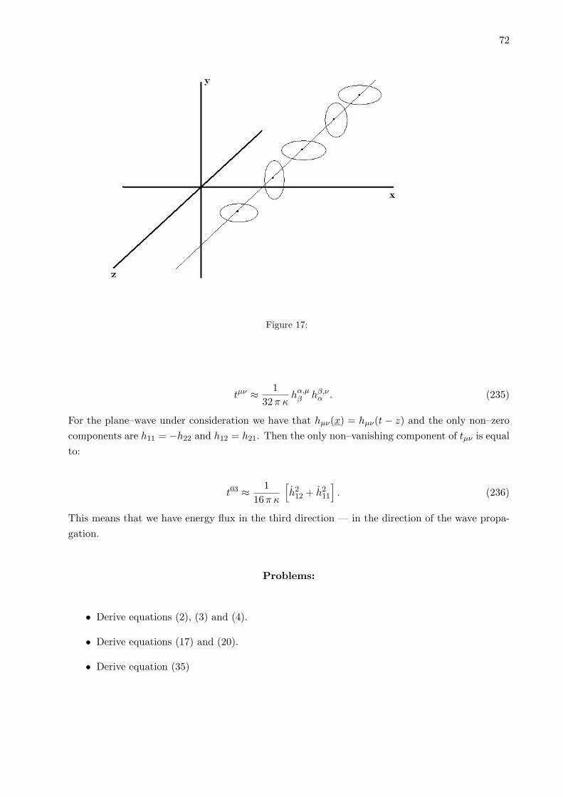
72

Figure 17:

tµν ≈ 132π κ

hα,µβ hβ,να . (235)

For the plane–wave under consideration we have that hµν(x) = hµν(t − z) and the only non–zerocomponents are h11 = −h22 and h12 = h21. Then the only non–vanishing component of tµν is equalto:

t03 ≈ 116π κ

[h2

12 + h211

]. (236)

This means that we have energy flux in the third direction — in the direction of the wave propa-gation.

Problems:

• Derive equations (2), (3) and (4).

• Derive equations (17) and (20).

• Derive equation (35)

73


• Linearized perturbations over the Schwarzschild background. (See e.g. “The mathematicaltheory of black holes”, S. Chandrasekhar, Oxford University Press, 1992)

74

LECTURE XGravitational radiation by moving massive bodies. Shock gravitational wave or Penrose parallel

plane wave.

1. In the previous lecture we have considered free gravitational waves. Here we continue withthe creation of such waves by massive bodies. Then, we have to solve the following equation:

−ψµν ≈ 16π κTµν , (237)

in the gauge ∂µψµν = 0, where

ψµν ≡ hµν −12ηµν h, and h ≡ hαα. (238)

Here Tµν is the matter stress–energy tensor, which contains terms that are ∼ O(h) and the gaugeunder consideration is in the agreement with the stress–energy conservation ∂µTµν = 0 in the linearapproximation.

Here we consider the creation of the radiation in the non–relativistic approximation. To solvethe eq. (237) one has to use the retarded Green function of the d’Alembert operator. From thecourse of classical electrodynamics it is known that this function is as follows:

GR(x− y

)= 4π δ(4)

(x− y

),

GR(x− y

)= Θ (tx − ty)

δ (tx − ty − |~x− ~y|)|~x− ~y|

, (239)

where Θ(t) is the Heaviside’s step function. Hence, the solution of (237) has the form:

ψµν (t, ~x) ≈ −4κ∫d3~y

Tµν (~y, t− |~x− ~y|)|~x− ~y|

. (240)

Suppose now that massive bodies, which create the radiation, perform their motion in a finiteregion V of the space, i.e. Tµν (ty, ~y) 6= 0 only if ~y ∈ V . We want to consider the gravitationalfield in the so called wave zone, i.e. very far away from the region where the radiation was created.Hence, in the above expressions we assume that |~x| |~y|, for ~y ∈ V . Then one can neglect y incomparison with x in the denominator of (240). Moreover, if we consider non–relativistic motionof the radiating bodies, then we also can neglect y in comparison with x in the argument of Tµνunder the integral in (240).

Thus, for |~x| |~y| the field in (240) actually solves the homogeneous form of the equation (237),i.e. with Tµν = 0, because we consider it outside the region V . As the result, the gravitationalfield, ψµν or hµν , in eq. (240) has the same properties as free waves of the previous lecture, i.e.hαα = 0 and ψµν = hµν . Moreover, the latter hµν has only spatially directed non–zero components.All in all the solution that we are looking for is as follows:

75

hij (t, ~x) ≈ −4κ|~x|

∫Vd3~y Tij (t, ~y) , i, j = 1, 2, 3. (241)

In this expression Tij depends on details of motion of radiating massive bodies rather than just ontheir mass distribution. To simplify this expression we will transform it into such a form that it willdepend only on the mass distribution. For this reason consider the spatial part of the stress–energyconservation: ∂µTµi(y) = 0. Multiply it by yj and integrate over a spatial section:

0 =∫d3~y yj ∂

µTµi =∫d3~y yj (∂tT0i − ∂kTki) . (242)

After the integration by parts in the second term in the last expression and dropping off theboundary term (as usual), we arrive at the following relation:

0 = ∂t

∫d3~y yj T0i +

∫d3~y Tji. (243)

Taking into account that Tij = Tji, we obtain the equation:

∫d3~y Tij = −1

2∂t

∫d3~y (yj T0i + yi T0j) . (244)

Similarly multiplying the equation ∂µTµ0 = 0 by yk yl and integrating over a spatial section wefind that:

0 =∫d3~y yk yl ∂

µTµ0 =∫d3~y yk yl (∂tT00 − ∂mTm0) = ∂t

∫d3~y yk yl T00 +

∫d3~y (yk T0l + yl T0k) .(245)

Thus, from these relations and from (241) we obtain that:

hij ≈ −2κ|~x|

∂2t

∫d3~y yi yj T00. (246)

Now take into account that for the non–relativistic system under consideration the T00 componentof the energy–momentum tensor coincides with the mass density: T00 ≈ ρ. Also in the wave zonehii = 0 and, hence, we can subtract from hij in eq. (246) its trace. As the result, we obtain that

hij ≈ −2κ

3 |~x|Qij , where

Qij ≡∫d3~y ρ (t, ~y)

(3 yi yj − δij ~y2

)(247)

is the quadruple moment of the mass distribution.This answer is quite natural and can be understood on general physical grounds. In fact,

in the case of electromagnetic radiation the corresponding vector field is proportional to the first

76

derivative of the dipole moment, Ai ∼ di. Hence, in the gravitational case it is natural to expect thatthe corresponding radiation tensor field is proportional to the second derivative of the quadruplemoment: hij ∼ Qij . Furthermore, in the electromagnetic case the electric and magnetic dipoleradiation vanish for such a system in which the gyromagnetic ratios e/m of all charges composingthe system are the same. The radiation type that is not zero in such a case is the quadruple one.But for the gravitational radiation the role of the charge is played by the mass. Hence, in such acase “e/m” is always the same. Then it is natural to expect that the quadruple radiation is thefirst non–zero contribution in the multiple expansion.

2. Let us find now the intensity of the radiation under consideration. As we have seen in theprevious lecture, if the radiated wave is traveling along the third direction, then:

t30 ≈1

32π κhij hij , (248)

and the indexes here run only over i, j = 1, 2. However, in generic situation waves are created byrandomly moving bodies and, then, radiation is going in all directions. Hence, we have to averagethe energy flux over all spatial directions. For that reason we need to find hij corresponding to awave which is traveling in an arbitrary direction specified by a unit vector ~n, ~n2 = 1. Such a hijtensor should be symmetric, hij = hji, traceless, hii = 0, and transversal to ~n, i.e. hij nj = 0. Thetransversal tensor has the following form:

h⊥ij = hij − ni nk hkj − nj nk hik + ni nj nk nl hkl. (249)

where hij is defined above. The transverse traceless tensor is then equal to:

hij = h⊥ij −12

(δij − ni nj) h⊥ll . (250)

From this equation and the condition that n2i = 1 we find:

hij hij = hij hij − 2ni nj hki hjk +12

(ni nj hij)2 . (251)

Taking into account the following expressions for the averages over all spatial directions:

〈ni nj〉 =13δij ,

〈ni nj nk nl〉 =115

(δij δkl + δik δjl + δil δjk) , (252)

we obtain that:

⟨hij hij

⟩=

25hij hij . (253)

77

Here:

〈ni1 . . . niN 〉 ≡1

4π

∫ 2π

0dϕ

∫ π

0dθ ni1 . . . niN and

~n = (sin(θ) cos(ϕ), sin(θ) sin(ϕ), cos(θ)) . (254)

Combining all these formulas together and using (247), we obtain the following expression for theradiation intensity:

I ≡∫dσi t

i0 ≈ 4π |~x|2 1

32π κ

⟨˙hij

˙hij

⟩≈ κ

45

...Qij

...Qij , (255)

where dσi = dΩ |~x|2 ni. This is the total intensity of the gravitational radiation in the quadrupleapproximation.

3. So far we have considered approximate solutions of the Einstein equations, which describeweak gravitational waves in the linearized approximation. In the remaining part of this lecture wepresent an exact solution describing so to say gravitational shock wave.

Consider the Schwarzschild metric and make the following change of the radial coordinate

r =(

1 +rg4ρ

)2

ρ.

Then the metric is transformed into the following form:

ds2 =

(1− rg

4ρ

1 + rg4ρ

)2

dt2 −(

1 +rg4ρ

)4 (dρ2 + ρ2 dΩ2

). (256)

In this metric the spatial part is conformaly flat. Hence, we can make a change from the sphericalcoordinates, (ρ, θ, ϕ), to the Cartesian ones (x, y, z): e.g., ρ2 = x2 + y2 + z2. Then, dρ2 + ρ2 dΩ2 =dx2 + dy2 + dz2.

Now we make a coordinate transformation, which describes the Lorentz boost along the z

direction:

t = γ t+ γ v z, and z = γ v t+ γ z, where γ =1√

1− v2. (257)

Because our metric is not Minkowskain such a transformation does change it. The new metricdescribes the motion of the black hole with the constant velocity v along the third direction. Thederivation of the explicit form of this metric is left as an exercise for the reader.

Now let us take the limit γ → ∞ (v → 1) and rg → 0 in such a way that rg γ2 ≡ κ p remains

finite. In this limit the Schwarzschild black hole is transformed to a solution describing a shockwave, which is moving with momentum p and with the speed of light along the z direction. Namely,in the limit under discussion the metric in (256) is reduced to

78

Figure 18:

ds2 = 2 du dv + 2H (u, ~x⊥) du2 − d~x2⊥, (258)

where

u =t− z√

2, v =

t+ z√2, ~x⊥ = (x, y), and H (u, ~x⊥) = κ p δ(u) log |~x⊥| . (259)

It is not hard to check that the only non–zero component of the Ricci tensor for (258) has thefollowing form — Ruu = ∆x⊥H (u, ~x⊥), where ∆x⊥ = ∂2

x + ∂2y .

The metric tensor (258) is the exact solution of the Einstein equations with the matter energy–momentum tensor equal to Tuu = p δ(u) δ(2) (~x⊥), because ∆x⊥ log |~x⊥| = 2π δ(2) (~x⊥). This solu-tion is referred to as Penrose parallel plane wave. The proof of all the above statements is left asan exercise for the reader. As it should be, such an energy–momentum tensor, Tuu, corresponds toa shock wave traveling with momentum p along the world line u = 0 and ~x⊥ = 0. The metric inquestion is defined beyond the world–line of the gravitational source, where there is the singularity.Note that the metric under consideration is not asymptotically flat and has a naked singularity.

4. Let us describe the behavior of light rays in the background of (258). Light rays which aremoving some distance, ~x⊥ = ~a (hence, d~x⊥ = 0), away from the source of the gravity are describedby the following equation:

0 = du [dv +H (u,~a) du] . (260)

79

Figure 19:

Hence, those light rays which are propagating parallel to the world–line of the shock wave, u = 0,(i.e. their world–line is u = const) never feel its influence and always travel according to the lawdu = 0. However, those light rays which collide with the shock wave, with the impact parameter~a, are moving along the world–line described by the equation:

dv = −κ p δ(u) log |~a| du. (261)

Before the collision with the wave (i.e. before u = 0) they move as if they are in flat space, dv = 0.(See the fig. (18).) During the collision the light is carried over by the shock wave for the distance

∫ 0+0

0−0duκ p δ(u) log |~a| = κ p log |~a| (262)

along the z direction. And then such a light ray is released to continue its free propagation accordingto the law dv = 0.

The reason for such a behavior of light rays in the background of the shock wave can beunderstood on general grounds. Field lines of a static massive body are spherically symmetric.However, after a boost, due to the Lorentz contraction, the density of these lines is increased in thedirections that are transversal to the boost axis. For a faster boost the density increase is stronger.See the fig. (19). In the case of the infinite boost one obtains so to say a pancake spanned in thedirections perpendicular to the propagation axis.

A light ray experiences a time delay while passing nearby a gravitating body: The main portionof the delay happens in the dense part of its field lines. As we boost the gravitating body the

80

region where the time delay is happening is shrinking. In the above defined limit the entire timedelay is happening when the light ray is crossing the shock wave (pancake), as is shown on the fig.(19).

Problems:

• Derive eq. (20).

• Derive eq. (22) from the eq. (20) in the limit γ →∞, rg → 0 and γ rg/2 ≡ κ p = const.

• Find the change in time of the radius of a double–star system due to the gravitationalradiation. (See the corresponding paragraph in Landau and Lifshitz)

• Find the resonance transformation of the high–energy electromagnetic wave into the gravi-tational one. (See the corresponding paragraph in Khriplovich book.)


• ADM gravitational mass and other definitions of the mass in the General theory of Relativity.

• Petrov’s classification of Einstein space–times.

• Gravitational memory and Bondi–Metzner–Sachs transformations at asymptotic infinity.

81

LECTURE XIHomogeneous three–dimensional spaces. Friedmann–Robertson–Walker metric. Homogeneous

isotropic cosmological solutions. Anisotropic Kasner cosmological solution.

1. At the scales of the Sun system our Universe is highly inhomogeneous. In fact, we seecompact gravitating bodies surrounded by large empty spaces. However, on scales of the orderof several hundreds of millions of parsecs (bigger than a characteristic size of galactic clusters)the distribution of matter in the Universe is isotropic and homogeneous. Moreover, observationaldata show that distant galaxies in all directions are running away from our own galaxy. In thislecture we would like to find solutions of Einstein equations which describe such a behavior of thehomogeneously distributed matter.

The most general four–dimensional metric tensor, which describes isotropic and homogeneousspatial sections as seen by inertial (free floating) observers, is as follows:

ds2 = dt2 − a2(t) γij(x) dxi dxj , i, j = 1, 2, 3. (263)

Here dl2 = γij(x) dxi dxj describes spatial sections and their size is changing according to the timedependence of a(t). Because of the homogeneity all points of spatial sections and all directionsfrom these points are equivalent to each other. Hence, the three–dimensional metric, dl2, underconsideration should correspond to a space of constant curvature.

2. Metric tensor in a space of constant curvature can be written as follows:

dl2 = γij(x) dxi dxj =dr2

1− k r2+ r2 dΩ2, dΩ2 = dθ2 + sin2 θ dϕ2. (264)

Here, k can be either −1, 0 or 1. In fact,

• When, k = 0 we have that dl2 = dr2 + r2 dΩ2, which is just the flat three–dimensionalEuclidian space represented in the spherical coordinates — the space of the constant zerocurvature.

• If k = 1, one deals with the metric:

dl2 =dr2

1− r2+ r2 dΩ2. (265)

After the coordinate change r = sinχ this metric is transformed into:

dl2 = dχ2 + sin2 χdΩ2, (266)

which is just the three–dimensional sphere — the space of constant positive unit curvature.We have encountered this metric in the lecture on the Oppenheimer–Snyder collapse.

82

For the future convenience let us point out here that the last metric is induced on the unitsphere

W 2 +X2 + Y 2 + Z2 = 1 (267)

embedded into the four–dimensional Euclidian space

dl24 = dW 2 + dX2 + dY 2 + dZ2. (268)

In fact, if one solves eq. (267) as (W,X, Y, Z) =(cosχ, sinχ sin θ cosϕ, sinχ sin θ sinϕ, sinχ cos θ) and, then, substitutes this into (268), heobtains the induced metric (266).

• Finally, for the case k = −1, we have to work with the metric as follows:

dl2 =dr2

1 + r2+ r2 dΩ2. (269)

If one will perform a coordinate change r = sinhχ, he will find that the metric is questionis transformed into:

dl2 = dχ2 + sinh2 χdΩ2. (270)

This metric can be obtained as follows. Consider the two–sheeted hyperboloid,

W 2 −X2 − Y 2 − Z2 = 1, (271)

embedded into the four–dimensional Minkowski space–time:

ds2 = dW 2 − dX2 − dY 2 − dZ2. (272)

One sheet of the hyperboloid corresponds to W ≥ 1, while the other — to W ≤ −1.The equation defining the hyperboloid under consideration is invariant under the Lorentzrotations, SO(3, 1), of the ambient Minkowski space. Hence, the whole hyperboloid can begenerated from a single point if one will act by the SO(3, 1) group. Moreover, an arbitrarypoint of this hyperboloid, say (W,X, Y, Z) = (1, 0, 0, 0), does not move under the actionof the SO(3) rotational subgroup of SO(3, 1) in the spatial, (X,Y, Z), part. As the resultthe hyperboloid is a homogeneous SO(3, 1)/SO(3) space. Hence, its every point and everydirection are equivalent to each other. Then the space has constant curvature. In fact,

83

the hyperboloid is just the three–dimensional Lobachevsky space — the space of constantnegative unit curvature.

One can solve the condition (271) as (W,X, Y, Z) =(coshχ, sinhχ sin θ cosϕ, sinhχ sin θ sinϕ, sinhχ cos θ). Then, after the substitutionof this solution into eq.(272), we obtain the metric tensor (270).

3. Thus, in this lecture we will work with the Friedmann–Robertson–Walker metric:

ds2 = dt2 − a2(t)[

dr2

1− k r2+ r2 dΩ2

]. (273)

The components of this metric tensor are:

g00 = 1, g11 = − a2

1− k r2, g22 = −a2 r2, g33 = −a2 r2 sin2 θ. (274)

At the same time, the inverse metric tensor is as follows:

g00 = 1, g11 = −1− k r2

a2, g22 = − 1

a2 r2, g33 = − 1

a2 r2 sin2 θ. (275)

Then the corresponding non–zero components of the Christoffel’s symbols (up to their symmetries)are:

Γ011 =

a a

1− k r2, Γ0

22 = r2 a a, Γ033 = r2 sin2 θ a a,

Γ101 =

a

a, Γ1

11 =k r

1− k r2, Γ1

22 = −r(1− k r2

), Γ1

33 = −r(1− k r2

)sin2 θ,

Γ202 =

a

a, Γ2

12 =1r, Γ2

33 = − sin θ cos θ,

Γ303 =

a

a, Γ3

13 =1r, Γ3

23 = cot θ. (276)

As the result the Ricci tensor has the form as follows:

R00 = −3 aa, R11 =

a a+ 2 a2 + 2 k1− k r2

,

R22 = r2(a a+ 2 a2 + 2 k

), R33 = r2 sin2 θ

(a a+ 2 a2 + 2 k

), (277)

and the Ricci scalar is equal to

R = −6a a+ a2 + k

a2. (278)

Here a ≡ da/dt and a ≡ d2a/dt2.

84

4. To find the dependence of the scale factor a on time we have to solve the Einstein equations.To do that one has to specify the matter energy–momentum tensor, which respects the symmetriesof the problem. The appropriate tensor was defined in one of the previous lectures and has thefollowing form:

Tµν = ρ(t)uµ uν + p(t) [uµ uν − gµν ] . (279)

The only peculiarity here, which is relevant for cosmology, is that ρ and p are functions of time only.For the free falling matter in the metric (273) its four–velocity is equal to uµ = (1, 0, 0, 0). Thenthe energy–momentum tensor has the form T νµ = Diag [ρ(t),−p(t),−p(t),−p(t)], which obviouslyrespects the homogeneity of spatial sections in the problem under consideration. In this lecture weset the cosmological constant Λ to zero.

Thus, we have that

T00 = ρ, T11 =p a2

1− k r2, T22 = p r2 a2, T33 = p r2 a2 sin2 θ, and

T 00 = ρ, T 11 =p(1− k r2

)a2

, T 22 =p

a2 r2, T 33 =

p

a2 r2 sin2 θ. (280)

Correspondingly the “00” and “11” components of the Einstein equations are as follows:

3(a2 + k

)= 8π κ ρ a2,

2 a a+ a2 + k = −8π κ p a2. (281)

These are referred to as Friedmann equations. The “22” and “33” components lead to the equationsthat are equivalent to the second relation in (281). That should be the case due to the symmetriesof the problem. Off diagonal components of the Einstein equations lead in this case to the trivialrelations of the form 0 = 0.

The temporal component of the energy–momentum conservation condition, DµTµ0 = 0, acquires

the form:

ρ+ 3 (p+ ρ)a

a= 0. (282)

Spatial components, DµTµj = 0, j = 1, 2, 3, of the conservation law lead to trivial relations. The

obtained equation (282) is not independent, but follows from (281). This should be the case,because, as was explained in the previous lectures, the energy–momentum conservation followsfrom the Einstein equations.

5. Let us consider various solutions of the above Friedmann’s equations for different choices ofequations of state p = p(ρ). The standard cosmological equation of state is as follows:

p = w ρ, where w = const. (283)

85

The two peculiar cases are represented by the choices w = 0 and w = 1/3. The first case w = 0 isthe familiar dust matter. In cosmology it describes galactic matter spread over the universe. Thesecond case, w = 1/3 corresponds, to the traceless, Tµµ = 0, stress–energy tensor. This situationone encounters, e.g., in the case of the Maxwell theory. Hence, this is said to correspond to theradiation.

For w = 0 the eq. (282) is reduced to ρ(t) · a3(t) = const, which just means that if the size ofspatial directions is scaling as a(t), i.e. if the spatial volume behaves as a3(t), then the density ofdust should change as ρ(t) ∼ 1/a3(t).

At the same time, when p = ρ/3 from (282) we obtain that ρ(t) ·a4(t) = const. The explanationof this relation is as follows. The density of photons is scaling in the same way as that of thedust ∼ 1/a3(t). But on top of that the wave length of photons is scaling as a(t). Hence, theirfrequency (or energy) is changing as 1/a(t). As the result, the photon’s energy density behaves asρ(t) ∼ 1/a4(t).

To solve the Friedmann’s equations it is convenient to change in (273) the time coordinateaccording to dt = a(η) dη. Then we obtain the metric as follows:

ds2 = a2(η)[dη2 − dr2

1− k r2− r2 dΩ2

], (284)

where η is the so called conformal time.From the first equation in (281) we find that:

dt = ± da√8π κ

3 a2 ρ− k. (285)

Here the “+” and “−” signs correspond to the solutions that are related to each other by thetime–reversal transformation. From this equation we find the conformal time:

η = ±∫

da

a√

8π κ3 a2 ρ− k

. (286)

Let us calculate this integral to obtain a(η) and then find t(η) from dt = a(η) dη for all six casesk = −1, 0, 1 and w = 0, 1/3. We restrict ourselves to the “+” sign in (286).

• If k = 1, w = 0, it is convenient to introduce the notations:

ρa3 ≡ M

2π2= const. (287)

Here we have introduced M , which is so to say the total mass of the compact Universe. Inthis case from (286) we obtain that

86

a(η) =2κM3π

(1− cos η) . (288)

Furthermore, from dt = a dη we find:

t(η) =2κM3π

(η − sin η) . (289)

This is the solution that we have encountered in the lecture on the Oppenheimer–Snydercollapse, but written in a bit different terms. The function a(t) starts its growth at t = 0(η = 0) as a(t) ∼ t2/3 for small t. Then, it approaches its maximal value, a = 4κM

3π , att = 2κM

3 (η = π). After that a(t) shrinks back to zero at t = 4κM3 (η = 2π). At the initial

expanding stage the energy–density behaves as ρ ∼ 1/t2.

• If k = 1, w = 1/3, we define:

ρ a4 ≡ 3 a21

8π κ= const. (290)

In this case from (286) we obtain:

a(η) = a1 sin η, t(η) = a1 (1− cos η) . (291)

Then, at the beginning of the expanding stage a(t) ∼√t and ρ ∼ 1/t2. Again in this case

the Universe starts its expansion from a = 0, reaches its maximal size and then shrinks back.

• If k = −1, w = 0, we introduce notations:

ρ a3 ≡ 3 a0

4π κ= const. (292)

Then,

a(η) = a0 (cosh η − 1) , t(η) = a0 (sinh η − η) , (293)

and in this case a(t) starts its homogeneous eternal growth at a = 0. At the initial stagea ∼ t2/3.

• If k = −1, w = 1/3, we define:

ρ a4 ≡ 3 a21

8π κ= const. (294)

87

Then,

a(η) = a1 sinh η, t(η) = a1 (cosh η − 1) . (295)

Again at the initial stage the spatial conformal factor starts as a(t) ∼√t and then a(t)

continues its eternal homogeneous growth.

• If k = 0, w = 0, then ρ a3 = const and directly from (285) it follows that for all times wehave that a(t) = const · t2/3.

• If k = 0, w = 1/3, as usual we have that ρ a4 = const and from (285) it follows that a(t) =const ·

√t.

With a good precision at this stage of its evolution our Universe corresponds to the case ofk = 0 and w = 0. At the same time at an early stage of its expansion there was a situation whenit was described by the case of k = 0 and w = 1/3. Recent observations show, however, that thecosmological constant is not zero, but is very small. This is so called dark energy. Its presence willchange the cosmological picture in the future of our Universe. We discuss these issues in the nextlecture.

In all the above cases the metric tensor degenerates at t = 0. This is the physical (curvaturerather than metric) singularity because it corresponds to the infinite energy density, ρ. Usuallythe problem of this initial singularity is solved via the assumption that the Universe had an ini-tial exponentially expanding stage, which is described by a space–time of constant curvature, i.e.again with non–zero cosmological constant. There are several observational signs approving thisassumption. We will discuss this type of space–times in the next lecture.

6. Let us consider here the simplest vacuum anisotropic (but spatially homogeneous) cosmo-logical solution. This is the so called Kasner solution.

Consider the metric of the form:

ds2 = dt2 −X2(t) dx2 − Y 2(t) dy2 − Z2(t) dz2. (296)

Note that if X = Y = Z = a we encounter the Friedmann–Robertson–Walker solution with k = 0.For such a metric the non–zero components of the Ricci tensor are as follows:

R00 = Θ +A2 +B2 + C2 and

R11 = −A−ΘA, R22 = −B −ΘB, R33 = −C −ΘC, (297)

where

A =X

X, B =

Y

Y, C =

Z

Z, and Θ ≡ A+B + C. (298)

88

The energy–momentum conservation condition is of the following form:

ρ+ Θ (p+ ρ) = 0. (299)

Because we consider the vacuum solution, Tµν = 0, the “00” component of the Einstein equationsleads to

0 = R00 −12R = −AB −BC − CA. (300)

As the result, from the definition of Θ we find that:

Θ2 = A2 +B2 + C2. (301)

Hence, using (297) from the equation

0 = R00 = Θ + Θ2 (302)

we deduce that

Θ =1

t− t0. (303)

By a choice of the origin we can set t0 = 0. Then,

0 = R11 = −A−AΘ, and A =p

t, (304)

for some constant p. Similarly we obtain

B =q

t, and C =

r

t, (305)

for some constants q and r. Next (301) and (303) with (298) imply that

p+ q + r = 1, and p2 + q2 + r2 = 1. (306)

And finally from A = X/X = p/t we obtain that X = X0 tp and similarly for Y and Z. Thus, the

Kasner’s metric can therefore be written as:

ds2 = dt2 − t2p dx2 − t2q dy2 − t2r dz2, (307)

after the appropriate rescalings of x, y and z. Here p, q and r are subject to (306).

89

7. Let us consider again the Schwarzschild black hole behind the event horizon. There onecan also use the same Schwarzschild metric, but with other t and r, which do not have an obviousrelation to the standard Schwarzschild coordinates:

ds2 =dr2

rgr − 1

−(rgr− 1)dt2 − r2 dΩ2, where r < rg. (308)

Here r plays the role of time, while t is space–like. The metric is time–dependent, it is notspherically symmetric and it is not asymptotically flat.

Consider the limit as r → 0. Then this metric simplifies to

ds2 ≈ r

rgdr2 − rg

rdt2 − r2 dΩ2. (309)

Making the change of variables:

√r

rgdr = dT,

(2 rg3

) 13

dt = dX,

(32√rg

) 23

dθ = dY,

(32√rg

) 23

dϕ = dZ, (310)

we arrive at the following form of this metric:

ds2 ≈ dT 2 − T− 23 dX2 − T

43 dY 2 − T

43 dZ2, (311)

for the case of small ϕ and θ. The reason why we can take ϕ, θ → 0 is because as T → 0, inthe approach towards the singularity, points that have large spatial separations (e.g., in ϕ and θ

directions) are causally disconnected.Thus, the obtained metric is nothing but the Kasner solution with T → 0. Hence, in the vicinity

of the physical singularity of the Schwarzschild black hole we have a Kasner type of the behaviorof the metric. This is actually a particular case of a more general situation: in the vicinity of anytime–like singularity one encounters Kasner type solution, which, however, does not necessarilyhave to be of the vacuum type.

Problems:

• Derive eq. (281) and eq. (282)

• Draw Penrose–Carter diagrams for all the homogeneous cosmological solutions.


90

• Linearized perturbations in cosmology. (See e.g. S.Weinberg, ”Cosmology”, Oxford Univer-sity Press, 2008.)

• Anisotropic cosmological solutions and cosmological billiards. (See e.g. “Cosmological bil-liards”, by T. Damour, M. Henneaux and H. Nicolai; Published in Class.Quant.Grav. 20(2003) R145-R200; e-Print: hep-th/0212256)

91

LECTURE XIIGeometry of the de Sitter space–time. Geometry of the anti–de Sitter space–time.

1. So far we always have been setting the cosmological constant, Λ, to zero. In this lecture wefind the most symmetric and simplest (so to say ground state) solutions of the Einstein equationsin the case when Λ 6= 0, but Tµν = 0. Note, however, that the standard energy–momentum tensor,

Tµν = ρ uµ uν + p (uµ uν − gµν) , (312)

with p = −ρ, i.e. w = −1, describes the same situation, Tµν = ρ gµν , as non–zero cosmologicalconstant, if ρ = const. Hence, one can find the metrics that are defined below using the methods ofthe previous lecture, but for many reasons we prefer the pure geometric picture/language adoptedhere.

D-dimensional space–time of constant curvature solves the following equation:

Gαβ = ±(D − 1)(D − 2)2

H2 gαβ, α, β = 0, . . . , D − 1. (313)

Here Gαβ is the Einstein tensor and H is the Hubble constant:

Λ =(D − 1) (D − 2)

2H2. (314)

In this equation “+” sign corresponds to the space–time of constant positive curvature. At thesame time “−” sign corresponds to the space–time of constant negative curvature. The reason forthat is explained below.

2. D-dimensional de Sitter space–time, that of the constant positive curvature, can be realizedas the following hyperboloid,

−(X0)2 +

(X1)2 + · · ·+

(XD

)2 ≡ −ηAB XAXB = H−2, A,B = 0, . . . , D, (315)

placed into the ambient (D + 1)-dimensional Minkowski space–time, with the metric ds2 =ηAB dX

A dXB. One way to see that a metric on such a hyperboloid solves equation (313) isto observe that it can be obtained from the sphere via the analytical continuation XD+1 → iX0.This is referred to as Wick rotation. In fact, after such a change of coordinates the ambientMinkowski space–time is transformed into the Euclidian one. At the same time, the equation (315)is transformed into the one defining D–dimensional sphere. Note that the Wick rotation does notchange the sign of the curvature.

For illustrative reasons we depict two-dimensional de Sitter space–time on the fig. (20). Hereeach constant X0 slice of this two-dimensional de Sitter space–time is the circle of the radius(H−2 +X2

0 ).

92

Another way to see that the hyperboloid in question has a constant curvature is to observethat eq. (315) is invariant under SO(D, 1) Lorentz transformations of the ambient space–time.The stabilizer of arbitrary point, say

(X0, X1, X2, . . . XD

)= (0, 1/H, 0, . . . , 0), obeying (315) is

SO(D − 1, 1) group. Hence, the de Sitter space–time is homogeneous, SO(D, 1)/SO(D − 1, 1),manifold and any its point is equivalent to another one. Furthermore, all directions at every pointare equivalent to each other up to the difference between space and time. (Compare this with thesphere, which is SO(D + 1)/SO(D).) Thus, SO(D, 1) Lorentz group of the ambient Minkowskispace is the de Sitter isometry group.

The geodesic distance, L12, between two points, XA1 and XA

2 , on the hyperboloid can be con-veniently expressed via the so-called hyperbolic distance, Z12, as follows:

cos (H L12)H2

≡ Z12

H2≡ −ηAB XA

1 XB2 , where − ηAB XA

1,2XB1,2 = H−2. (316)

To better understand the meaning of this expression, it is instructive to compare it to the geodesicdistance, l12, on a sphere of radius R:

R2 cos(l12

R

)≡ R2 z12 ≡

(~X1

~X2

), where ~X2

1,2 = R2.

While the spherical distance, z12, is always less than unity, the hyperbolic one, Z12, can acquireany value because of the Minkowskian signature of the metric.

All geodesics on the hyperboloid of fig. (20) are curves that are cut out on it by planes goingthrough the origin of the ambient Minkowski space–time. (The situation here is absolutely sim-ilar to the case of the sphere, as can be understood after the Wick rotation.) Hence, space-likegeodesics are ellipses, time-like ones are hyperbolas and light-like are straight generatrix lines ofthe hyperboloid, which are also light–like in the ambient Minkowski space–time.

2. To define a metric on the de Sitter space–time, which is induced from the ambient space,one has to find a solution of eq. (315). One possibility is as follows

X0 =sinh(Ht)

H, Xi =

ni cosh(Ht)H

, i = 1, . . . , D (317)

where ni is a unit, n2i = 1, D-dimensional vector. One can choose:

n1 = cos θ1, −π2≤ θ1 ≤

π

2n2 = sin θ1 cos θ2, −π

2≤ θ2 ≤

π

2. . . (318)

nD−2 = sin θ1 sin θ2 . . . sin θD−3 cos θD−2, −π2≤ θD−2 ≤

π

2nD−1 = sin θ1 sin θ2 . . . sin θD−2 cos θD−1, −π ≤ θD−1 ≤ π

nD = sin θ1 sin θ2 . . . sin θD−2 sin θD−1.

93

Figure 20:

Then, the induced metric is:

ds2 = dt2 − cosh2(Ht)H2

dΩ2D−1, (319)

where

dΩ2D−1 =

D−1∑j=1

(j−1∏i=1

sin2 θi

)dθ2j (320)

is the line element on the unit (D − 1)-dimensional sphere. The metric (319) covers the de Sitterspace–time totaly and is referred to as global. Its constant t slices are compact (D−1)-dimensionalspheres. Note that one can obtain from (319) the metric of the D-dimensional sphere after theanalytical continuation, H t→ i

(θD − π

2

), which is the same as above Wick rotation.

The hyperbolic distance in these coordinates is given by:

Z12 = − sinh(Ht1) sinh(Ht2) + cosh(Ht1) cosh(Ht2) cos(ω), (321)

where cos(ω) = (~n1, ~n2).3. To understand the causal structure of the de Sitter space–time it is convenient to transform

the global coordinates as follows:

94

Figure 21:

cosh2(Ht) =1

cos2 θ, −π

2≤ θ ≤ π

2,

and to obtain the metric:

ds2 =1

H2 cos2 θ[dθ2 − dΩ2

D−1

]. (322)

If D > 2, then to draw the diagram on the two-dimensional sheet we should choose, in additionto θ, one of the angles θj , j = 1, . . . , D − 1. The usual choice is θ1 because the metric in questionhas the form dθ2 − dθ2

1 − sin2(θ1)dΩ2D−2, i.e., it is flat in the (θ − θ1)-plain. The Penrose–Carter

diagram for the de Sitter space–time, whose dimension is grater than 2, is depicted on the fig. (21).The straight thin line here is the constant t and/or θ slice.

Note that when D > 2 angle θ1 is taking values in the range[−π

2 ,π2

]. At the same time,

when D = 2 we have that θ1 ∈ [−π, π]. When D > 2, the problem with the choice of θ1 in thePenrose–Carter diagram is that then cylindrical topology, SD−1 × R, of the de Sitter space–timeis not transparent. At the same time, the complication with the choice of θD−1 ∈ [−π, π], insteadof θ1, appears form the fact that the metric in the (θ − θD−1)–plain is not flat, if D > 2. For thisreason we prefer to consider just the stereographic projection in the two-dimensional case becauseit is sufficient to describe the causal structure and also clearly shows the topology of the de Sitterspace–time.

The Penrose–Carter diagram of the two-dimensional de Sitter space–time is shown on the fig.(22). This is the stereographic projection of the hyperboloid from the fig. (20). What is depicted

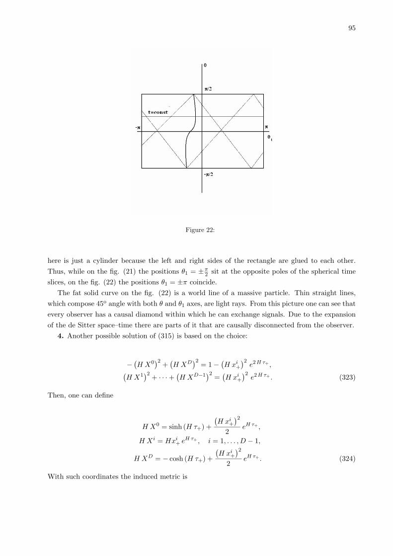
95

Figure 22:

here is just a cylinder because the left and right sides of the rectangle are glued to each other.Thus, while on the fig. (21) the positions θ1 = ±π

2 sit at the opposite poles of the spherical timeslices, on the fig. (22) the positions θ1 = ±π coincide.

The fat solid curve on the fig. (22) is a world line of a massive particle. Thin straight lines,which compose 45o angle with both θ and θ1 axes, are light rays. From this picture one can see thatevery observer has a causal diamond within which he can exchange signals. Due to the expansionof the de Sitter space–time there are parts of it that are causally disconnected from the observer.

4. Another possible solution of (315) is based on the choice:

−(HX0

)2 +(HXD

)2= 1−

(H xi+

)2e2H τ+ ,(

HX1)2 + · · ·+

(HXD−1

)2=(H xi+

)2e2H τ+ . (323)

Then, one can define

HX0 = sinh (H τ+) +

(H xi+

)22

eH τ+ ,

H X i = Hxi+ eH τ+ , i = 1, . . . , D − 1,

H XD = − cosh (H τ+) +

(H xi+

)22

eH τ+ . (324)

With such coordinates the induced metric is

96

Figure 23:

ds2+ = dτ2+ − e2H τ+ d~x2

+. (325)

Note, however, that in (324) we have the following restriction: −X0 +XD = − 1H eH τ+ ≤ 0, i.e.,

metric (325) covers only half, X0 ≥ XD, of the entire de Sitter space–time. It is referred toas the expanding Poincare patch (EPP). Another half of the de Sitter space–time, X0 ≤ XD, isreferred to as the contracting Poincare patch (CPP) and is covered by the metric

ds2− = dτ2− − e−2H τ− d~x2

−. (326)

In both patches it is convenient to change the proper time τ± into the conformal one. Then, theEPP and CPP both possess the same metric:

ds2± =1

(H η±)2[dη2

± − d~x2±], H η± = e∓H τ± . (327)

However, while in the EPP the conformal time is changing form η+ = +∞ at past infinity (τ+ =−∞) to 0 at future infinity (τ+ = +∞), in the CPP the conformal time is changing from η− = 0at past infinity (τ− = −∞) to +∞ at future infinity (τ− = +∞). Both the EPP and CPP areshown on the fig. (23). The boundary between the EPP and CPP is light-like and is situated atη± = +∞. We also show on this picture the constant conformal time slices.

97

The hyperbolic distance in the EPP and CPP has the form:

Z12 = 1 +(η1 − η2)

2 − |~x1 − ~x2|2

2 η1 η2. (328)

It is worth mentioning here that it is possible to cover simultaneously the EPP and CPP with theuse of the metric (327), if one makes the changes ~x± → ~x and η± → η ∈ (−∞,+∞). Then, whileat the negative values of the conformal time, η = −η+ < 0, it covers the EPP, at its positive values,η = η− > 0, this metric covers the CPP. The inconvenience of such a choice of global metric is dueto that the boundary between the EPP and CPP simultaneously corresponds to η = ±∞.

5. We define here the physical and comoving spatial volumes in global de Sitter space–timeand in its Poincare patches. The spatial sections in all aforementioned metrics contain conformalfactors, cosh2(H t)

H2 or 1(H η±)2

. Then, there is the volume form, dD−1V , with respect to the spatialmetric, which is multiplying the corresponding conformal factor. This form remains constantduring the time evolution of the spatial sections and is referred to as comoving volume.

It is important to observe that if one considers a dust in the de Sitter space–time, then its densityper comoving volume remains constant independently of whether spatial sections are expanding orcontracting.

At the same time if one takes into account the conformal factor, i.e., the expansion (contraction)of the EPP (CPP), then he has to deal with the physical volume, dD−1V±

(H η±)D−1 . In the global de Sitter

space–time the physical volume is coshD−1(H t) dD−1Vsphere

HD−1 . Of course the density of the dust withrespect to such a volume is changing in time.

6. The case of anti–de Sitter space–time is very similar to the de Sitter one. However, thereare certain differences. D–dimensional anti–de Sitter is the hyperboloid,

−X20 +

D−1∑j=1

X2j −X2

D = − 1H2

, (329)

embedded into the (D + 1)–dimensional space–time of (+,−, . . . ,−,+) signature:

ds2 = dX20 −

D−1∑j=1

dX2j + dX2

D. (330)

Hence, the isometry of the hyperboloid (329) is SO(D−1, 2), while the stabilizer of a generic pointis SO(D−1, 1). Hence, the anti–de Sitter space–time is homogeneous, SO(D−1, 2)/SO(D−1, 1),manifold.

Under the Wick rotation XD → iXD we obtain the two–sheeted hyperboloid,

−X20 +

D∑j=1

X2j = − 1

H2or

D∑j=1

X2j = X2

0 −1H2

,

98

Figure 24:

embedded into the (D + 1)–dimensional Minkowski space–time:

ds2 = dX20 −

D∑j=1

dX2j .

This two–sheeted hyperboloid is the constant negative curvature D–dimensional Lobachevski spaceof Euclidian signature. The three–dimensional version of this space we have encountered in theprevious lecture.

Note that after the redefinitions X ↔ iX and H ↔ iH we can map all the above definedD–dimensional space–times, D–dimensional sphere and D–dimensional Lobachevski space to eachother. The redefinition H → iH changes the sign of the curvature. Hence, similarly to the sphereand to the de Sitter space–time one can define here the hyperbolic distance both in the Lobachevskispace and in the anti–de Sitter space–time. Moreover, this way one also can define the geodesicsin Lobachevski space and anti–de Sitter space–time.

7. Solving eq. (329) as

X0 =1H

cosh ρ cos τ XD =1H

cosh ρ sin τ,

Xj =1H

sinh ρnj , n2j = 1, j = 1, . . . , D − 1, (331)

and plaguing this solution into (330), we obtain the following induced metric on the anti–de Sitterspace–time:

99

Figure 25:

ds2 =1H2

[cosh2 ρ dτ2 − dρ2 − sinh2 ρ dΩ2

D−2

]. (332)

Here τ ∈ [0, 2π) and dΩ2D−2 is the metric on the (D−2)–dimensional sphere, which is parameterized

by nj . In the case when D = 2 the coordinate ρ is ranging from −∞ to +∞. Then constant timeτ slices are just hyperbolas. The two–dimensional anti–de Sitter space–time looks just as the deSitter one, but rotated by the angle π/2 around the X2 axis. See the fig. (24).

When D > 2 the range of values of ρ is [0,+∞). Only in such a case we cover entire anti–deSitter space and avoid double–counting. Then constant time τ slices are Lobachevski hyperboloidswith the metric

dl2 =1H2

[dρ2 + sinh2 ρ dΩ2

D−2

]. (333)

The three–dimensional variant of this metric (with H = 1 and ρ→ χ) we have encountered in theprevious lecture. Here ρ = 0 is just the center of the hyperboloid in question.

Note that above defined time τ is compact, τ ∈ [0, 2π). Which can be seen on the fig. (24).This is physically unfavorable situation. Hence, in physics literature one usually considers universalcover of the space–time under consideration, i.e. the metric (332) with τ ∈ (−∞,+∞). The spatialboundary, ρ→ +∞, of such a space–time is conformaly equivalent to the cylinder R×SD−2. HereR is for the axis of time τ and SD−2 is for the sphere described by the metric dΩ2

D−2.8. To draw the Penrose–Carter diagram of the anti–de Sitter space–time, one can make the

following change of variables:

tan θ = sinh ρ, and ds2 =1

H2 cos2 θ[dτ2 − dθ2 − sin2 θ dΩ2

D−2

].

100

Figure 26:

Here if D = 2, then θ ∈ [−π/2, π/2], while for the case of D > 2 one has to deal with θ ∈ [0, π/2]because of the above mentioned difference of the range of values of ρ. Then the Penrose–Carterdiagram for the case of D = 2 is the same as for the two–dimensional de Sitter space–time, whichis, however, rotated by the π/2 angle around the axis perpendicular to the plane of the picture.That is the stereographic projection of the hyperboloid from the fig. (24). Thus, two–dimensionalanti–de Sitter space–time has two boundaries — at θ = −π/2 and θ = π/2.

At the same time the Penrose–Carter diagram for the case of D > 2 is shown on the fig.(25). On this picture θ = π/2 is the spatial boundary of the anti–de Sitter space, but θ = 0 isnot a boundary, rather it corresponds to ρ = 0, which is the center of the (D − 1)–dimensionalLobachevski space, which is represented by the metric (333). The Lobachevski space topologicallyis just a ball.

Also on the fig. (25) we show light rays and a world–line of a massive particle by the straightand curly thin curves, correspondingly. As can be seen from this picture, starting at any internalpoint, light rays can reach the spatial boundary of the space–time within finite coordinate andproper times.

As the result to solve a Cauchy problem in the anti–de Sitter space–time one has to specifyboundary conditions on top of the initial ones. Consider the fig. (26). Indeed, to solve a physicalproblems one deals with causal differential equations. Then to find a value of the solution at apoint O one needs to know its behavior in the grey causal triangle, which is bounded by the pastlight–cone. In the absence of a boundary this behavior is totaly defined by initial values given atthe Cauchy surface Σ. In the case under study, however, we encounter such a situation that a partof the boundary B can lay in the causal past of an internal point. That is the reason one has theabove mentioned complication of the Cauchy problem in anti–de Sitter space–time. This propertyis referred to as the absence of global hyperbolicity. Rephrasing this, anti–de Sitter space–timeacts as a box: its gravity is such that it attracts back massive particles when they try to escape to

101

the spatial infinity. But for light rays we have to specify boundary conditions at spatial infinity:e.g. that could be of mirror type or say absorbing boundaries.

9. Let us describe the Poincare patch and Poincare coordinates of the anti–de Sitter space–time.Let us solve the eq. (329) as follows:

X0 =z

2

[1 +

1z2

(1H2− xµ xµ

)], z ≥ 0,

X1 =z

2

[1− 1

z2

(1H2

+ xµ xµ

)]Xµ =

xµH z

, µ = 2, . . . , D. (334)

Here xµxµ = ηµνxµxν and ||ηµν || = Diag(−,−, . . . ,−,+).

This is very similar to the choice of coordinates that we have made in the Poincare patch ofthe de Sitter space–time. To see that one just has to make the change z → η = e−Hτ . Note thathere X0 − X1 = 1

(Hz)2≥ 0. Hence, these coordinates cover only half of the entire anti–de Sitter

space–time.As the result from (330) we obtain the induced metric as follows:

ds2 =1

(H z)2[dz2 + dxµ dx

µ]. (335)

It is very similar to the metric on the Poincare patch of the de Sitter space–time, but with onecrucial difference that while η is time and, hence, the de Sitter metric is time dependent, z is spatialcoordinate. The time coordinate of the anti–de Sitter space–time is hidden in dxµ dxµ ≡ d~x2−dt2.Thus, both the anti–de Sitter space–time and its Poincare patch are static.

Problems:

• Derive the metric (14) from eq. (13).

• Derive the metric (24) from eq. (23).


• Harmonics and Green’s functions in homogeneous spaces of constant curvature. (For the caseof de Sitter space–time see e.g. “Lecture notes on interacting quantum fields in de Sitterspace”, by E.T. Akhmedov; Published in Int.J.Mod.Phys. D23 (2014) 1430001; e-Print:arXiv:1309.2557 )

• Anti–de Sitter isometry group and the conformal group action on its boundary.

102

• Conformal embeddings (C. Fefferman, C.R. Graham, Conformal invariants, in: Elie Cartanet les Mathmatiques d’ajourd’hui, Astrisque (hors srie) Socit Mathmatique de France, Paris,1985, pp. 95116.)

Documents

Lectures on General Theory of Relativity1 To my mother Lectures on General Theory of Relativity Emil T. Akhmedov These lectures are based on the following books: •Textbook On Theoretical