Embed Size (px)
Citation preview
Lectures on Algebraic Groups
Alexander Kleshchev

Contents
Part one: Algebraic Geometry page 11 General Algebra 32 Commutative Algebra 52.1 Some random facts 52.2 Ring extensions 83 Affine and Projective Algebraic Sets 183.1 Zariski topology 183.2 Nullstellensatz 203.3 Regular functions 223.4 Irreducible components 233.5 Category of algebraic sets 253.6 Products 283.7 Rational functions 293.8 Projective n-space 323.9 Functions 343.10 Product of projective algebraic sets 353.11 Example: Grassmann varieties and flag varieties 363.12 Example: Veronese variety 393.13 Problems 414 Varieties 464.1 Affine varieties 464.2 Prevarieties 494.3 Products 514.4 Varieties 534.5 Dimension 544.6 Problems 605 Morphisms 635.1 Fibers 63
iii

iv Contents
5.2 Finite morphisms 645.3 Image of a morphism 665.4 Open and birational morphisms 695.5 Problems 706 Tangent spaces 726.1 Definition of tangent space 726.2 Simple points 746.3 Local ring of a simple point 766.4 Differential of a morphism 776.5 Module of differentials 786.6 Simple points revisited 836.7 Separable morphisms 856.8 Problems 877 Complete Varieties 887.1 Main Properties 887.2 Completeness of projective varieties 89
Part two: Algebraic Groups 918 Basic Concepts 938.1 Definition and first examples 938.2 First properties 958.3 Actions of Algebraic Groups 988.4 Linear Algebraic Groups 1008.5 Problems 1029 Lie algebra of an algebraic group 1059.1 Definitions 1059.2 Examples 1079.3 Ad and ad 1089.4 Properties of subgroups and subalgebras 1109.5 Automorphisms and derivations 1119.6 Problems 11210 Quotients 11410.1 Construction 11410.2 Quotients 11510.3 Normal subgroups 11810.4 Problems 12011 Semisimple and unipotent elements 12111.1 Jordan-Chevalley decomposition 12111.2 Unipotent algebraic groups 12411.3 Problems 125

Contents v
12 Characteristic 0 theory 12712.1 Correspondence between groups and Lie algebras 12712.2 Semisimple groups and Lie algebras 12912.3 Problems 13013 Semisimple Lie algebras 13113.1 Root systems 13113.2 Semisimple Lie algebras 13413.3 Construction of simple Lie algebras 13713.4 Kostant Z-form 13913.5 Weights and representations 14013.6 Problems 14214 The Chevalley construction 14514.1 Definition and first properties 14615 Borel subgroups and flag varieties 14815.1 Complete varieties and Borel’s fixed point theorem 14815.2 Borel subgroups 14915.3 The Bruhat order 15116 The classification of reductive algebraic groups 15416.1 Maximal tori and the root system 15416.2 Sketch of the classification 156Bibliography 160


Part one
Algebraic Geometry


1
General Algebra
Definition 1.0.1 A functor F : A → B is called faithful if the map
HomA(A1, A2)→ HomB(F (A1), F (A2)), θ 7→ F (θ) (1.1)
is injective, and F is called full if the map (1.1) is surjective.
Theorem 1.0.2 A functor F : A → B is an equivalence of categories ifand only if the following two conditions hold:
(i) F is full and faithful;(ii) every object of B is isomorphic to an object of the form F (A) for
some A ∈ ObA.
Proof ( ⇒ ) Let F be an equivalence of categories and G : B → Abe the quasi-inverse functor. Let α : GF → idA and β : FG → idBbe isomorphisms of functors. First of all, for any object B of B βB :F (G(B)) → B is an isomorphism, which gives (ii). Next, for each ϕ ∈HomA(A1, A2) we have the commutative diagram
GF (A1) A1
GF (A2) A2
?
GF (ϕ)
-αA1
?
ϕ
-αA2
Hence ϕ can be recovered from F (ϕ) by the formula
ϕ = αA2 GF (ϕ) (αA1)−1. (1.2)
This shows that F is faithful. Similarly, G is faithful. To prove that F
3

4 General Algebra
is full, consider an arbitrary morphism ψ ∈ HomB(F (A1), F (A2)), andset
ϕ := αA2 G(ψ) (αA1)−1 ∈ HomA(A1, A2).
Comparing this with (1.2) and taking into account that αA1 and αA2
are isomorphisms, we deduce that G(ψ) = GF (ϕ). As G is faithful,this implies that ψ = F (ϕ), which completes the proof that F is a fullfunctor.
( ⇐ ) Assume that (i) and (ii) hold. In view of (i), we can (and will)identify the set HomB(F (A1), F (A2)) with the set HomA(A1, A2) forany A1, A2 ∈ ObA. Using (ii), for each object B in B we can pick anobject AB in A and an isomorphism βB : F (AB) → B. We define afunctor G : B → A which will turn out to be a quasi-inverse functor toF . on the objects we set G(B) = AB for any B ∈ ObB. To define G onthe morphisms, let ψ ∈ HomB(B1, B2).
G(ψ) := β−1B2 ψ βB1 ∈HomB(FG(B1), FG(B2))
= HomA(G(B1), G(B2)).
It is easy to see that G is a functor, and β = βB : FG → idB isan isomorphism of functors. Further, βF (A) = F (αA) for the uniquemorphism αA : GF (A) → A. Finally, it is not hard to see that α =αA : GF → idA is an isomorphism of functors.

2
Commutative Algebra
Here we collect some theorems from commutative algebra which are notalways covered in 600 algebra. All rings and algebras are assumed to becommutative.
2.1 Some random facts
Lemma 2.1.1 Let k be a field, f, g ∈ k[x, y], and assume that f isirreducible. If g is not divisible by f , then the system f(x, y) = g(x, y) =0 has only finitely many solutions.
Proof See [Sh, 1.1].
Proposition 2.1.2 Let A,B be k-algebras, I / A, J / B be ideals. Then
A/I ⊗k B/J → (A⊗k B)/(A⊗ J + I ⊗B), a⊗ b 7→ a⊗ b
is an isomorphism of algebras.
Definition 2.1.3 A subset S of a commutative ring R is called multi-plicative if 1 ∈ S and s1s2 ∈ S whenever s1, s2 ∈ S. A multiplicativesubset is called proper if 0 6∈ S.
Lemma 2.1.4 Let S ⊂ R be a proper multiplicative set. Let I be anideal of R satisfying I ∩ S = ∅. The set T of ideals J ⊇ I such thatJ ∩ S = ∅ has maximal elements, and each maximal element in T is aprime ideal.
5

6 Commutative Algebra
Proof That the set T has maximal elements follows from Zorn Lemma.Let M be such an element. Assume that x, y ∈ R \M . By the choice ofM , M + Rx contains some s1 ∈ S and M + Ry contains some s2 ∈ S,i.e. s1 = m1 + r1x and s2 = m2 + r2y. Hence
s1s2 = (m1 + r1x)(m2 + r2y) ∈M +Rxy.
It follws that M +Rxy 6= M , i.e. xy 6∈M .
Theorem 2.1.5 (Prime Avoidance Theorem) Let P1, . . . , Pn beprime ideals of the ring R. If some ideal I is contained in the unionP1 ∪ · · · ∪ PN , then I is already contained in some Pi.
Proof We can assume that none of the prime ideals is contained inanother, because then we could omit it. Fix an i0 ∈ 1, . . . , N and foreach i 6= i0 choose an fi ∈ Pi, fi 6∈ Pi0 , and choose an fi0 ∈ I, fi0 6∈ Pi0 .Then hi0 :=
∏fi lies in each Pi with i 6= i0 and I but not in Pi0 . Now,∑
hi lies in I but not in any Pi.
Lemma 2.1.6 (Nakayama’s Lemma) Let M be a finitely generatedmodule over the ring A. Let I be an ideal in A such that for any a ∈ 1+I,aM = 0 implies M = 0. Then IM = M implies M = 0.
Proof Let m1, . . . ,ml be generators of M . The condition IM = M
means that
mi =l∑
j=1
xijmj (1 ≤ i ≤ l).
for some xij ∈ I. Hence
l∑j=1
(xij − δij)mj = 0 (1 ≤ i ≤ l).
So by Cramer’s rule, dmj = 0, where d = det(xij − δij). Hence dM = 0.But d ∈ 1 + I, so M = 0.
Corollary 2.1.7 If B ⊃ A is a ring extension, and B is finitely gener-ated as an A-module, then IB 6= B for any proper ideal I of A.
Proof Since B contains 1, we have aB = 0 only if a = 0. Now allelements of 1 + I are non-zero for a proper ideal I, so we can applyNakayama’s Lemma.

2.1 Some random facts 7
Corollary 2.1.8 (Nakayama’s Lemma) Let M be a finitely generatedmodule over the ring A, M ′ ⊆ M be a submodule, and let I be an idealin A such that all elements of 1 + I are invertible. Then IM +M ′ = M
implies M ′ = M .
Proof Apply Lemma 2.1.6 to M/M ′.
Another version:
Corollary 2.1.9 (Nakayama’s Lemma) Let M be a finitely generatedmodule over a ring A, and I be a maximal ideal of A. If IM = M , thenthere exists x 6∈M such that xM = 0.
Proof Localize at I and apply Corollary 2.1.8.
Corollary 2.1.10 Let M be a finitely generated module over the ring Aand let I be an ideal in A such that all elements of 1 + I are invertible.Then elements m1, . . . ,mn ∈M generate M if and only if their imagesgenerate M/IM .
Proof Apply Corollary 2.1.8 to M ′ = (m1, . . . ,mn).
Lemma 2.1.11 Let M be a maximal ideal of R, then the map R →RM induces the isomorphism of the fields R/M and RM/MRM . If weidentify the fields via this isomorphism, then the the map R→ RM alsoinduces the isomorphism of vector spaces M/M2 →MRM/(MRM )2.
A field extension K/k is called separable, if either char k = 0 orchar k = p > 0 and for any k-linearly independent elements x1, . . . , xn ∈K, we have xp1, . . . , x
pn are linearly independent. A filedK = k(x1, . . . , xn)
is called separably generated over k if K is a finite separable extensionof a purely transcendental extension of k.
Theorem 2.1.12
(i) The extension K = k(x1, . . . , xn)/k is separably generated if andonly if K/k is separable.
(ii) If k is perfect (in particular algebraically closed), then any fieldextension K/k is separable.
(iii) Let F/K/k be field extensions. If F/k is separable, then K/k isseparable. If F/K and K/k are separable, then F/k is separable.
8 Commutative Algebra
Theorem 2.1.13 (Primitive Element Theorem) If K/k is a finiteseparable extension, then there is an element x ∈ K such that K = k(x).
Let L/E be a field extension. A derivation is a map δ : E → L suchthat
δ(x+ y) = δ(x) + δ(y) and δ(xy) = xδ(y) + δ(x)y (x, y ∈ E).
If F is a subfield of E, then the derivation δ is F -derivation if it is F -linear. The space DerF (E,L) of all F -derivations is a vector space overL. With this notation, we have:
Theorem 2.1.14
(i) If E/F is separably generated then
dim DerF (E,L) = tr.degF E.
(ii) E/F is separable if and only all derivations F → L extend toderivations E → L.
(iii) If charE = p > 0, then all derivations are zero on the subfieldEp. In particular, if E is perfect, all derivations of E are zero.
Theorem 2.1.15 [Ma, Theorem 20.3] A regular local ring is a UFD. Inparticular it is an integrally closed domain.
2.2 Ring extensions
Definition 2.2.1 A ring extension of a ring R is a ring A of which R isa subring.
If A is a ring extension of R, A is a fathful R-module in a natural way.Let A be a ring extension of R and S be a subset of A. The subringof A generated by R and S is denoted R[S]. It is quite clear that R[S]consists of all R-linear combinations of products of elements of S.
Definition 2.2.2 A ring extension A of R is called finitely generated ifA = R[s1, . . . , sn] for some finitely many elements s1, . . . , sn ∈ A.
The following notion resembles that of an algebraic element for fieldextensions.

2.2 Ring extensions 9
Definition 2.2.3 Let A be a ring extension of R. An element α ∈ A iscalled integral over R if f(α) = 0 for some monic polynomial f(x) ∈ R[x].A ring extension R ⊆ A is called integral if every element of A is integralover R.
In Proposition 2.2.5 we give two equivalent reformulations of the in-tegrality condition. For the proof we will need the following technical
Lemma 2.2.4 Let V be an R-module. Assume that v1, . . . , vn ∈ V andaij ∈ R, 1 ≤ i, j ≤ n satisfy
∑nj=1 akjvj = 0 for all 1 ≤ k ≤ n. Then
D := det(aij) satisfies Dvi = 0 for all 1 ≤ i ≤ n.
Proof We expand D by the ith column to get D =∑nk=1 akiCki, where
Cki is the (k, i) cofactor. We then also have∑nk=1 akjCki = 0 for i 6= j.
So
Dvi =n∑k=1
akiCkivi =n∑k=1
akiCkivi +∑j 6=i
(n∑k=1
akjCki)vj
=n∑j=1
n∑k=1
akjCkivj =n∑k=1
Cki
n∑j=1
akjvj = 0.
Proposition 2.2.5 Let A be a ring extension of R and α ∈ A. Thefollowing conditions are equivalent:
(i) α is integral over R.(ii) R[α] is a finitely generated R-module.(iii) There exists a faithful R[α]-module which is finitely generated as
an R-module.
Proof (i) ⇒ (ii) Assume f(α) = 0 , where f(x) ∈ R[x] is monic ofdegree n. Let β ∈ R[α]. Then β = g(α) for some g ∈ R[x]. As f ismonic, we can write g = fq+r, where deg r < n. Then β = g(α) = r(α).Thus R[α] is generated by 1, α, . . . , αn−1 as an R-module.
(ii) ⇒ (iii) is clear.(iii) ⇒ (i) Let V be a faithful R[α]-module which is generated as an
R-module by finitely many elements v1, . . . , vn. Write
αvi = ai1v1 + · · ·+ ainvn (1 ≤ i ≤ n).

10 Commutative Algebra
Then
−ai1v1 − · · · − ai,i−1vi−1 + (α− aii)vi − ai,i+1vi+1 − · · · − ainvn = 0
for all 1 ≤ i ≤ n. By Lemma 2.2.4, we have Dvi = 0 for all i, where
D =
∣∣∣∣∣∣∣∣∣α− a11 −a12 · · · −a1n
−a21 α− a22 · · · −a2n
......
......
−an1 an2 · · · α− ann
∣∣∣∣∣∣∣∣∣ .As v1, . . . , vn generate V , this implies that D annihilates V . As V isfaithful, D = 0. Expanding D shows that D = f(α) for some monicpolynomial f(x) ∈ R[x].
Lemma 2.2.6 Let R ⊆ A ⊆ B be ring extensions. If A is finitelygenerated as an R-module and B is finitely generated as an A-module,then B is finitely generated as an R-module.
Proof If a1, . . . , am are generators of the R-module A and b1, . . . , bnare generators of the A-module B, then it is easy to see that aibj aregenerators of the R-module B.
Proposition 2.2.7 Let A be a ring extension of R.
(i) If A is finitely generated as an R-module, then A is integral overR.
(ii) If A = R[α1, . . . , αn] and α1, . . . , αn are integral over R, then A
is finitely generated as an R-module and hence integral over R.(iii) If A = R[S] and every s ∈ S is integral over R, then A is integral
over R.
Proof (i) Let α ∈ A. Then A is a faithful R[α]-module, and we canapply Proposition 2.2.5.
(ii) Note that R[α1, . . . , αi] = R[α1, . . . , αi−1][αi]. Now apply induc-tion, Proposition 2.2.5 and Lemma 2.2.6.
(iii) Follows from (ii).
Corollary 2.2.8 Let A be a ring extension of R. The elements of Awhich are integral over R form a subring of A.
Proof If α1, α2 ∈ A are integral, then α1 − α2 and α1α2 belong toR[α1, α2]. So we can apply Proposition 2.2.7(ii).

2.2 Ring extensions 11
This result allows us to give the following definition
Definition 2.2.9 The integral closure of R in A ⊇ R is the ring R of allelements of A that are integral over R. The ring R is integrally closedin A ⊇ R in case R = R. A domain R is called integrally closed if it isintegrally closed in its field of fractions.
Example 2.2.10 The elements of the integral closure of Z in C arecalled algebraic integers. They form a subring of C. In fact the field ofalgebraic numbers A is the quotient field of this ring.
We record some further nice properties of integral extensions.
Proposition 2.2.11 Let R,A,B be rings.
(i) If R ⊆ A ⊆ B then B is integral over R if and only if B isintegral over A and A is integral over R.
(ii) If B is integral over A and R[B] makes sense then R[B] is integralover R[A].
(iii) If A is integral over R and ϕ : A → B is a ring homomorphismthen ϕ(A) is integral over ϕ(R).
(iv) If A is integral over R, then S−1A is integral over S−1R for everyproper multiplicative subset S of R.
Proof (i)-(iii) is an exercise.(iv) First of all, it follows from definitions that S−1R is indeed a
subring of S−1A. Now, let [as ] ∈ S−1A. As [as ] = [a1 ][ 1s ], it suffices to
show that both [a1 ] and [ 1s ] are integral over S−1R. But 1s ∈ S
−1R andfor [a1 ] we can use the monic polynomial which annihilates a.
It follows from Proposition 2.2.11(i) that the closure of R in A ⊇ R isagain R. In particular, if D is any domain and F is its field of fractions,then the closure D in F is an integrally closed domain (since the quotientfield of D is also F ).
We recall that a domain R is called a unique factorization domain orUFD if every non-zero non-unit element of R can be written as a productof irreducible elements, which is unique up to a permutation and units.
Proposition 2.2.12 Every UFD is integrally closed.
Proof Let R be a UFD and F be its field of fractions. Let ab ∈ F be
integral over R. We may assume that no irreducible element of R divides

12 Commutative Algebra
both a and b. There is a monic polynomial f(x) = xn+rn−1xn−1+ · · ·+
r0 ∈ R[x] with f(ab ) = 0, which implies an+ rn−1an−1b+ · · ·+ r0b
n = 0.So, if p ∈ R is an irreducible element dividing b then p divides an, andhence p divides a, a contradiction. Therefore b is a unit and a
b ∈ R.
Proposition 2.2.13 If a domain R is integrally closed, then so is S−1R
for any proper multiplicative subset S of R.
Proof Exercise.
Example 2.2.14 The ring Z[i] of Gaussian integers is Euclidean (thedegree function is ∂(a + bi) = a2 + b2, hence it is a UFD, and so it isintegrally closed by Proposition 2.2.13. On the other hand consider thering Z[2i]. The quotient field of both Z[i] and Z[2i] is Q(i), and we haveZ[2i] ⊂ Z[i] ⊂ Q[i]. Clearly Z[2i] is not integrally closed, as i 6∈ Z[2i] isintegral over it. It is easy to see that Z[2i] = Z[i].
Theorem 2.2.15 If R is integrally closed, then so is R[x1, . . . , xr].
Next we are going to address the question of how prime ideals of Rand A are related if A ⊇ R is an integral extension.
Definition 2.2.16 Let R ⊆ A be a ring extension. We say that a primeideal P of A lies over a prime ideal p of R if P ∩R = p.
The following lemma is a key technical trick.
Lemma 2.2.17 Let A ⊇ R be an integral ring extension, p be a primeideal of R, and S := R \ p.
(i) Let I be an ideal of A avoiding S, and P be an ideal of A maximalamong the ideals of A which contain I and avoid S. Then P isa prime ideal of A lying over p.
(ii) If P is a prime ideal of A which lies over p, then P is maximalin the set T of all ideals in A which avoid S.
Proof (i) Clearly, S is a proper multiplicative subset of A. So P is primein view of Lemma 2.1.4. We claim that P ∩ R = p. That P ∩ R ⊆ p isclear as P ∩ S = ∅.
Assume that P ∩ R ( p. Let c ∈ p \ P . By the maximality of P ,p+ αc = s ∈ S for some p ∈ P and α ∈ A. As A is integral over R, we

2.2 Ring extensions 13
have
0 = αn + rn−1αn−1 + · · ·+ r0
for some r0, . . . , rn−1 ∈ R. Multiplying by cn yields
0 = cnαn + crn−1cn−1αn−1 + · · ·+ cnr0
= (s− p)n + crn−1(s− p)n−1 + · · ·+ cnr0.
If we decompose the last expression as the sum of monomials, then thepart which does not involve any positive powers of p looks like
x := sn + crn−1sn−1 + · · ·+ cnr0.
It follows that x ∈ P . On the other hand, x ∈ R, so x ∈ R ∩ P ⊆ p.Now c ∈ p implies sn ∈ p. As p is prime, s ∈ p, a contradiction.
(ii) If P is not maximal in T , then there exists an ideal I in T whichproperly contains P . As I still avoids S, it also lies over p. Take u ∈ I\P .Then u 6∈ R and u is integral over R. So the set of all polynomialsf ∈ R[x] such that deg f ≥ 1 and f(u) ∈ P is non-empty. Take suchf(x) =
∑ni=0 rix
i of minimal possible degree. We have
un + rn−1un−1 + · · ·+ r0 ∈ P ⊆ I,
whence r0 ∈ R ∩ I = p = R ∩ P ⊆ P . Therefore
un + rn−1un−1 + · · ·+ r1u = u(un−1 + rn−1u
n−2 + · · ·+ r1) ∈ P.
By the choice of u and minimality of deg f , u 6∈ P and un−1+rn−1un−2+
· · ·+ r1 6∈ P . We have contradiction because P is prime.
Corollary 2.2.18 (Lying Over Theorem) If A is integral over P thenfor every prime ideal p of R there exists a prime ideal P of A which liesover p. More generally, for every ideal I of A such that I ∩R ⊆ p thereexists a prime ideal P of A which contains I and lies over p.
Corollary 2.2.19 (Going Up Theorem) Let A ⊇ R be an integralring extension, and p1 ⊆ p2 be prime ideals in R. If P1 is a prime idealof A lying over p1, then there exists a prime ideal P2 of A such thatP1 ⊆ P2 and P2 lies over p2.
Proof Take p = p2 and I = P1 in Lemma 2.2.17(i).

14 Commutative Algebra
Corollary 2.2.20 (Incomparability) Let A ⊇ R be an integral ringextension, and P1, P2 be prime ideals of A lying over a prime ideal p ofR. Then P1 ⊆ P2 implies P1 = P2.
Proof Use Lemma 2.2.17(ii).
The relation between prime ideals established above has further niceproperties.
Theorem 2.2.21 (Maximality) Let A ⊇ R be an integral ring exten-sion, and P be a prime ideal of A lying over a prime ideal p of R. ThenP is maximal if and only if p is maximal.
Proof If p is not maximal, we can find a maximal ideal m ) p. Bythe Going Up Theorem, there is an ideal M of A lying over m andcontaining P . It is clear that M actually containg P properly, and so Pis not maximal.
Conversely, let p be maximal in R. Let M be a maximal ideal con-taining P . Then M ∩ R ⊇ P ∩ R = p and we cannot have M ∩ R = R,as 1R = 1S 6∈M . It follows that M ∩R = p. Now M = P by Incompa-rability Theorem.
The previous results can be used to prove some useful properties con-cerning extensions of homomorphisms.
Lemma 2.2.22 Let A ⊇ R be an integral ring extension. If R is a fieldthen A ⊇ R is an algebraic field extension.
Proof Let α ∈ A be a non-zero element. Then α is algebraic over R,hence R[α] ⊆ A is a field, and α is invertible. Hence A is a field.
Proposition 2.2.23 Let A be integral over R. Every homomorphism ϕ
of R to an algebraically closed field F can be extended to A.
Proof If R is a field, then A is an algebraic field extension of R byLemma 2.2.22. Now the result follows from Proposition ??.
If R is local, then kerϕ is the maximal ideal m of R. By Lying Overand Maximality Theorems, there is an ideal M of A lying over m. Theinclusion R → A then induces an embedding of fields R/m → A/M ,which we use to identify R/m with a subfield of A/M . Note that thefield extension A/M ⊇ R/m is algebraic. Since kerϕ = m, ϕ factors

2.2 Ring extensions 15
through the projection R → R/m. The resulting homomorphism ϕ :R/m → F can be extended to ψ : A/M → F by Proposition ??. Nowif π : A → A/M is the natural projection, then ψ π is the desiredextension of ϕ.
Now we consider the general case. Let p := kerϕ, a prime idealin R, and S = R \ p. Then S−1A is integral over S−1R by Proposi-tion 2.2.11(iv). Now S−1R = Rp is local. By the universal property oflocalizations, ϕ extends to a ring homomorphism ϕ : S−1R → F . Bythe local case, ϕ extends to ψ : S−1A → F , and the desired extensionψ : A→ F is obtained by composing ψ with the natural homomorphismA→ S−1A.
Proposition 2.2.24 Every homomorphism of a field k into an alge-braically closed field can be extended to every finitely generated ring ex-tension of k.
Proof Let ϕ : k → F be a homomorphism to an algebraically closedfield F and R be a finitely generated ring extension of k, so that R =k[α1, . . . , αn] for some α1, . . . , αn ∈ R.
First assume that R is a field. By Proposition 2.2.23, we may as-sume that R is not algebraic over k. Let β1, . . . , βt be a (necessarilyfinite) transcendence base of R over k. Each α ∈ R is algebraic overk(β1, . . . , βt), i.e. satisfies a polynomial akαk + · · ·+ a1α+ a0 = 0 withcoefficients ak, . . . , a0 ∈ k(β1, . . . , βt), ak 6= 0. Multiplying by a commondenominator yields a polynomial equation
bkαk + · · ·+ b1α+ b0 = 0
with coefficients bk, . . . , b0 ∈ k[β1, . . . , βt], bk 6= 0. Hence α is in-tegral over k[β1, . . . , βt,
1bk
]. Applying this to α1, . . . , αn yields non-zero c1, . . . , cn ∈ k[β1, . . . , βt] such that α1, . . . , αn are integral overk[β1, . . . , βt,
1c1, . . . , 1
cn]. Set c = c1 . . . cn. Then α1, . . . , αn are inte-
gral over k[β1, . . . , βt,1c ], and hence R is integral over k[β1, . . . , βt,
1c ],
see Proposition 2.2.7(ii). Let cϕ be the image of c under the homomor-phism
k[β1, . . . , βt] ∼= k[x1, . . . , xt]→ F [x1, . . . , xt]
induced by ϕ. As F is infinite there exist γ1, . . . , γt ∈ F such thatcϕ(γ1, . . . , γt) 6= 0. By the universal property of polynomial rings, thereexists a homomorphism ψ : k[β1, . . . , βt]→ F which extends ϕ and sends

16 Commutative Algebra
β1, . . . , βt to γ1, . . . , γt, respectively. The universal property of localiza-tions yields an extension of ψ to ring k[β1, . . . , βt,
1c ] = k[β1, . . . , βt]c.
Now Proposition 2.2.23 extends ϕ to R, which completes the case whereR is a field.
Now, let R = k[α1, . . . , αn] be any finitely generated ring extensionof k. Let m be a maximal ideal of R and π : R → R/m be the naturalprojection. Then R/m is a field extension of π(k) ∼= k generated byπ(α1), . . . , π(αn). By the first part of the proof, every homomorphismof π(k) into F extends to R/m. Therefore every homomorphism ofk ∼= π(k) extends to R.
Let K/k be a finite field extension. Consider K as a k-vector space.Then the map x 7→ ax is a k-linear map of this vector space. Define thenorm NK/k(a) to be the determinant of this map. Note that NK/k|K× :K× → k× is a group homomorphism.
Lemma 2.2.25 If a = a1, . . . , as be the roots with multiplicity of theminimal polynomial irr (a, k) (in some extension of the field K), thenNK/k(a) = (
∏si=1 ai)
[K:k(a)].
Proof If 1 = v1, v2, . . . , vr is a basis of K over k(u), then aivj | 0 ≤i < s, 1 ≤ j ≤ r is a basis of K over k in which the matrix of the mapx 7→ ax is block diagonal with blocks all equal to the companion matrixof irr (a, k).
Lemma 2.2.26 Let S ⊆ R be integral domains with fields of fractionsk ⊆ K, S be integrally closed, and r ∈ R be integral over S. Thenirr (r, k) ∈ S[x].
Proof Let F be an extension of K which contains all roots r = r1, . . . , rsof irr (r, k). Then each ri is integral over S. So the coefficients of irr (r, k),being polynomials in the ri are also integral over S. As S is integrallyclosed, the coefficients belong to S.
Corollary 2.2.27 Let S ⊆ R be domains with fields of fractions k ⊆ Ksuch that the field extension K/k is finite. Assume that the ring exten-sion S ⊆ R is integral and that S is integrally closed. Then NK/k(r) ∈ Sfor any r ∈ R.
Proof Apply Lemmas 2.2.25 and 2.2.26.

2.2 Ring extensions 17
Lemma 2.2.28 (Noether’s Normalization Lemma) Let k be a field,and R = k[x1, . . . , xn] be a domain, finitely generated over k with thefield of fractions F . If tr.degk F = d, then there exist algebraicallyindependent over k elements S1, . . . , Sd ∈ R such that R is integral overk[S1, . . . , Sd].
Theorem 2.2.29 (Going Down Theorem) Let S ⊆ R be an integralring extension and S be integrally closed. Let P1 ⊇ P2 be prime idealsof S, and Q1 be a prime ideal of R lying over P1. Then there exists aprime ideal Q2 ⊆ Q1 lying over P2.
3
Affine and Projective Algebraic Sets
3.1 Zariski topology
Algebraic geometry is the subject which studies (algebraic) varieties.Naively, varieties are just algebraic sets.
Throughout we fix an algebraically closed ground field k. (It is muchharder to develop algebraic geometry over non-algebraically closed fieldsand we will not try to do this). Denote by An the affine space kn—thisis just the set of all n-tuples of elements of k.
Definition 3.1.1 Let S ⊂ k[T1, . . . , Tn]. A zero of the set S is anelement (x1, . . . , xn) of An such that f(x1, . . . , xn) = 0 for all f ∈ S.The zero set of S is the set Z(S) of all zeros of S. An algebraic set inAn (or affine algebraic set) is the zero set of some set S ⊂ k[T1, . . . , Tn],in which case S is called a set of equations of the algebraic set.
Example 3.1.2 The straight line x+y−1 = 0 and the ‘circle’ x2 +y2−1 = 0 are examples of algebraic sets in C2. More generally, algebraicsets in C2 with a single equation are called complex algebraic curves.Note that the curve given by the equation (x+ y − 1)(x2 + y2 − 1) = 0is the union of the line and the ‘circle’ above. On the other hand, thezero set of x+y−4, x2 +y2−1 consists of two points (1, 0) and (0, 1).Finally, two more examples: ∅ = Z(1), and C2 = Z(0).
Note that Z(S) = Z((S)), where (S) is the ideal of k[T1, . . . , Tn] gen-erated by S. Therefore every algebraic set is the zero set of some ideal.Since k[T1, . . . , Tn] is noetherian by Hilbert’s Basis Theorem, every al-gebraic set is the sero set of a finite set of polynomials.
Example 3.1.3 Let us try to ‘classify’ algebraic sets in A1 and A2.
18

3.1 Zariski topology 19
(i) Algebraic sets in A1 are A1 itself and all finite subsets (including∅).
(ii) Let X be an algebraic set in A2. It is given by a system ofpolynomial equations: f1(T1, T2) = · · · = fm(T1, T2) = 0. If allpolynomials are zero, we get X = A2. If f1, . . . , fm do not have acommon divisor, then our system has only finitely many solutions,see Lemma 2.1.1. Finally, let all fi have greatest common divisord(T1, T2). Then fi = dgi, where the polynomials gi(T1, T2) do nothave a common divisor. Now, X = X1 ∪X2, where X1 is givenby the system g1 = · · · = gm = 0, and X2 is given by d = 0. Asabove X1 is a finite (possibly empty) set of points, while X2 isgiven by one non-trivial equation d = 0 (and can be thought ofas a ‘curve’ in A2).
Proposition 3.1.4
(i) Every intersection of algebraic sets is an algebraic set; the unionof finitely many algebraic sets is an algebraic set.
(ii) An and ∅ are algebraic sets in An.
Proof (i) Let (Xj = Z(Ij))j∈J be a family of algebraic sets, given aszero sets of certain ideals Ij . To see that their intersection is again analgebraic set, it is enough to note that ∩j∈JZ(Ij) = Z(
∑j∈J Ij). For
the union, let Z(I) and Z(J) be algebraic sets corresponding to ideals Iand J , and note that Z(I) ∪ Z(J) = Z(I ∩ J) (why?).
(ii) An = Z(0) and ∅ = Z(1).
The proposition above shows that algebraic sets in An are closed setsof some topology. This topology is called the Zariski topology. Zariskitoplology on An also induces Zariski topology on any subset of An, inparticular algebraic set. This topology is very weird and it takes timeto get used to it. The main unintuitive thing here is that the topologyis ‘highly non-Hausdorf’—its open sets are huge. For example, we sawabove that proper closed sets in k are exactly the finite sets, and so anytwo non-empty open sets intersect non-trivially.
Let f ∈ k[T1, . . . , Tn]. The corresponding principal open set is An \Z(f) = x ∈ An | f(x) 6= 0. It is easy to see that each open set inAn is a finite union of principal open sets, so principal open sets form abase of Zariski topology.

20 Affine and Projective Algebraic Sets
3.2 Nullstellensatz
The most important theorem of algebraic geometry is called Hilbert’sNullstellensatz (or theorem on zeros). It has many equivalent reformula-tions and many corollaries. The idea of the theorem is to relate algebraicsets in An (geometry) and ideals in k[T1, . . . , Tn] (commutative algebra).We have two obvious maps
Z : ideals in k[T1, . . . , Tn] → algebraic sets in An
and
I : algebraic sets in An → ideals in k[T1, . . . , Tn].
We have already defined Z(J) for an ideal J in k[T1, . . . , Tn]. As for I,let X be any subset of An. Then the ideal I(X) is defined to be
I(X) := f ∈ k[T1, . . . , Tn] | f(x1, . . . , xn) = 0 for all (x1, . . . , xn) ∈ X.
Lemma 3.2.1 Let X be any subset of An. Then Z(I(X)) = X, theclosure of X in Zariski topology. In particular, if X is an algebraic set,then Z(I(X)) = X.
Proof We have to show that for any algebraic set Z(J) containing X weactually have Z(I(X)) ⊆ Z(J). Well, as X ⊆ Z(J), we have I(X) ⊇ J ,which in turn implies Z(I(X)) ⊆ Z(J).
Note, however, that Z and I do not give us a one-to one correspon-dence. For example, in A1 we have Z((T )) = Z((T 2)) = 0, that isthe different ideals (T ) and (T 2) give the same algebraic set. Also, notethat I(0) = (T ) 6= (T 2). Nullstellensatz sorts out problems like thisin a very satisfactory way.
The first formulation of the Nulltellensatz is as follows (don’t forgetthat k is algebraically closed, otherwise the theorem is wrong):
Theorem 3.2.2 (Hilbert’s Nullstellensatz) Let J be an ideal ofk[T1, . . . , Tn]. Then I(Z(J)) =
√J .
Proof First of all, it is easy to see that√J ⊆ I(Z(J)). Indeed, let
f ∈√J . Then fn ∈ J . Then fn is zero at every point of Z(J). But
this implies that f is zero at every point of Z(J), i.e. f ∈ I(Z(J)).The converse is much deeper. Let f ∈ I(Z(J)) and assume that no
power of f belongs to J . Applying Lemma 2.1.4 to the multiplicativeset 1, f, f2, . . . yields a prime ideal P containing J but not f . Let

3.2 Nullstellensatz 21
R = k[T1, . . . , Tn]/P and π : k[T1, . . . , Tn] → R be the natural pro-jection. Then R is a domain which is generated over π(k) ∼= k byα1 := π(T1), . . . , αn := π(Tn). We identify k and π(k), and so π canbe considered as a homomorphism of k-algebras. Under this agreement,y := f(α1, . . . , αn) = π(f) 6= 0, non-zero element of R, as f 6∈ P .
By Proposition 2.2.24, the identity isomorphism k → k can be ex-tended to a homomorphism ψ from the subring k[α1, . . . , αn,
1y ] of the
fraction field of R to k. Then ψ(y) 6= 0. So
f(ψ(α1), . . . , ψ(αn)) = ψ(f(α1, . . . , αn)) = ψ(y) 6= 0.
On the other hand, for any g ∈ J ⊆ P we have
g(ψ(α1), . . . , ψ(αn)) = ψ(g(α1, . . . , αn)) = ψ(g(π(T1), . . . , π(Tn)))
= ψ(π(g(T1, . . . , Tn))) = ψ(π(g)) = ψ(0) = 0.
Thus (ψ(α1), . . . , ψ(αn)) is a zero of J but not of f , i.e. f 6∈ I(Z(J)), acontradiction.
Definition 3.2.3 We say that an ideal I of a commutative ring R isradical if
√I = I.
The following corollary is also often called Nullstellensatz.
Corollary 3.2.4 The maps I and Z induce an order-reversing bijectionbetween algebraic sets in An and radical ideals in k[T1, . . . , Tn].
Proof Note that I(X) is always a radical ideal for any subset X ⊆ An.Now the result follows from Theorem 3.2.2 and Lemma 3.2.1.
Corollary 3.2.5 Let J1 and J2 be two ideals of k[T1, . . . , Tn]. ThenZ(J1) = Z(J2) if and only if
√J1 =
√J2.
Proof It is clear that Z(J) = Z(√J) for any ideal J , which gives the
‘if’-part. The converse follows from Theorem 3.2.2.
Corollary 3.2.6 Every proper ideal of k[T1, . . . , Tn] has at least onezero in An.
Proof If√I = k[T1, . . . , Tn], then I = k[T1, . . . , Tn]. Now the result
follows from above.

22 Affine and Projective Algebraic Sets
Let x = (x1, . . . , xn) ∈ An. Denote I(x) by Mx, i.e.
Mx = f ∈ k[T1, . . . , Tn] | f(x1, . . . , xn) = 0.
Corollary 3.2.7 The mapping x 7→Mx is a one-to-one correspondencebetween An and the maximal ideals of k[T1, . . . , Tn].
Proof Note that the maximal ideals are radical and apply Nullstellen-satz.
3.3 Regular functions
Let X ⊆ An be an algebraic set. Every polynomial f ∈ k[T1, . . . , Tn]defines a k-valued function on An and hence on X via restriction. Suchfunctions are called regular functions on X. The regular functions forma k-algebra with respect to the obvious ‘point-wise operations’. Thealgebra is called the coordinate algebra (or coordinate ring) of X (orsimply the algebra/ring of regular functions on X) and denoted k[X].Clearly,
k[X] ∼= k[T1, . . . , Tn]/I(X).
If I is an ideal of k[X] then we write Z(I) for the set of all points x ∈ Xsuch that f(x) = 0 for every f ∈ I, and if Z is a subset of X we denoteby I(Z) the ideal of k[X] which consists of all functions f ∈ k[X] suchthat f(z) = 0 for every z ∈ Z. Note that closed subsets of X all looklike Z(I).
Now the Nullstellensatz and the correspondence theorem for idealsimply:
Theorem 3.3.1 (Hilbert’s Nullstellensatz) Let X be an algebraicset.
(i) If J is an ideal of k[X], then I(Z(J)) =√J .
(ii) The maps I and Z induce an order-reversing bijection betweenclosed sets in X and radical ideals in k[X].
(iii) Every proper ideal of k[X] has at least one zero in X.(iv) The mapping x 7→ Mx = f ∈ k[X] | f(x) = 0 is a one-to-one
correspondence between X and the maximal ideals of k[X].
Definition 3.3.2 A commutative finitely generated k-algebra withoutnilpotent elements is called an affine k-algebra.

3.4 Irreducible components 23
Proposition 3.3.3
(i) Let X be an algebraic set. Then k[X] is an affine k-algebra.(ii) Every affine k-algebra A is isomorphic to k[X] for some affine
algebraic set X.
Proof (i) clear. For (ii), if A = k[α1, . . . , αn] is an k-algebra generatedby α1, . . . , αn, then by the universal property of polynomial rings, A ∼=k[T1, . . . , Tn]/I for some radical ideal I. So I = I(X) for some algebraicset X by the Nulltellensatz.
Let f ∈ k[X]. The corresponding principal open set is
Xf := X \ Z(f) = x ∈ X | f(x) 6= 0. (3.1)
Each open set in X is a finite union of principal open sets, so principalopen sets form a base of Zariski topology.
Example 3.3.4
(i) If X is a point, then k[X] = k.(ii) If X = An, then k[X] = k[T1, . . . , Tn].(iii) Let X ⊂ A2 be given by the equation T1T2 = 1. Then k[X] is
isomorphic to the localization k[t]t ∼= k[t, t−1].
3.4 Irreducible components
Definition 3.4.1 A topological space is noetherian if its open sets satisfythe ascending chain condition.
A topological space is irreducible if it cannot be written as a union ofits two proper closed subsets.
Note that a non-empty open subset of an irreducible topological spaceX is dense inX, and that any two non-empty open subsets ofX intersectnon-trivially. Problem 3.13.18 contains some further important proper-ties of irreducible spaces.
Lemma 3.4.2 An with Zariski topology is noetherian. Hence the sameis true for any subspace of An.
Proof An ascending chain of open sets corresponds to a descendingchain of closed sets, which, by the Nullstellensatz, corresponds to an

24 Affine and Projective Algebraic Sets
ascending chain of radical ideals of k[T1, . . . , Tn], which stabilizes sincek[T1, . . . , Tn] is noetherian.
Lemma 3.4.3 Algebraic set X ⊆ An is irreducible if and only if theideal I(X) is prime.
Proof If X is irreducible and f1, f2 ∈ k[T1, . . . , Tn] with f1f2 ∈ I(X),then X ⊆ Z((f1)) ∪ Z((f2)), and we deduce that X ⊆ Z((f1)) or X ⊆Z((f2)), i.e. f1 ∈ I(X) or f2 ∈ I(X).
Conversely, if I(X) is prime and X = X1 ∪ X2 for proper closedsubsets X1, X2, then there are polynomials fi ∈ I(Xi) with fi 6∈ I(X).But f1f2 ∈ I(X), contradiction.
Since prime ideals are radical, Lemma 3.4.3 allows us to further re-fine the one-to-one correspondence between radical ideals and algebraicsets: under this correspondence prime ideals correspond to irreduciblealgebraic sets. Also note that X is irreducible if and only if k[X] is adomain. So for irreducible algebraic sets X we can form the quotientfield of k[X] is called the field of rational functions on X and denotedk(X). In a natural way, k(X) is a field extension of k.
We now establish a general fact on noetherian topological spaces,which in some sense reduces the study of algebraic sets to that of ir-reducible algebraic sets.
Proposition 3.4.4 Let X be a noetherian topological space. Then X
is a finite union X = X1 ∪ · · · ∪ Xr of irreducible closed subsets. Ifone assumes that Xi 6⊆ Xj for all i 6= j then the Xi are unique up topermutation. They are called the irreducible components of X and canbe characterized as the maximal irreducible closed subsets of X.
Proof Let X be a topological noetherian space for which the first state-ment is false. Then X is reducible, hence X = X1 ∪ X ′
1 for properclosed subsets X1, X
′1. Moreover, the first statement is false for at
least one of X1, X′1. Continuing this way, we get an infinite chain
X ) X1 ) · · · ) X2 ) . . . of closed subsets, which is a contradiction, asX is noetherian.
To show uniqueness, assume that we have two irredundant decom-positions X = X1 ∪ · · · ∪ Xr and X = X ′
1 ∪ · · · ∪ X ′s. For each i,
Xi ⊆ (X ′1 ∩Xi) ∪ · · · ∪ (X ′
s ∩Xi), so by irreducibility of Xi we may as-sume thatXi ⊆ X ′
σ(i) for some σ(i). For the same reason, X ′j ⊆ Xτ(j) for

3.5 Category of algebraic sets 25
some τ(j). Now the irredundancy of the decompositions implies that σand τ are mutually inverse bijections between 1, . . . , r and 1, . . . , s,and Xi = X ′
σ(i) for all i.
3.5 Category of algebraic sets
We now define morphisms between algebraic sets. Let X ⊆ An, Y ⊆ Ambe two algebraic sets and consider a map ϕ : X → Y . Let T1, . . . , Tnand S1, . . . , Sm be the coordinate functions on An and Am, respectively.Denote Si ϕ by ϕi for all 1 ≤ i ≤ m. So that we can think of ϕas the m-tuple of functions ϕ = (ϕ1, . . . , ϕm), where ϕi : X → k, andϕ(x) = (ϕ1(x), . . . , ϕm(x)) ∈ Am. The map ϕ : X → Y is calleda morphism of algebraic sets or a regular map from X to Y if eachfunction ϕi : X → k, 1 ≤ i ≤ n is a regular function on X. It is easy tosee that algebraic sets and regular maps form a category, in particulara composition of regular maps is a regular map again.
Now, let ϕ : X → Y be a morphism of algebraic sets as above. Thismorphism defines the ‘dual’ morphism ϕ∗ : k[Y ] → k[X] of coordinatealgebras, as follows:
ϕ∗ : k[Y ]→ k[X] : f 7→ f ϕ.
It is clear that ϕ∗ is a homomorphism of k-algebras. Moreover, (ϕψ)∗ =ψ∗ ϕ∗ and id∗ = id, i.e. we have a contravariant functor F fromthe category of algebraic sets to the category of affine k-algebras. Toreiterate: F(X) = k[X] and F(ϕ) = ϕ∗.
Theorem 3.5.1 The functor F from the category of algebraic sets (overk) to the category of affine k-algebras is a (contravariant) equivalence ofcategories.
Proof In view of Theorem 1.0.2 (for contravariant functors) and Propo-sition 3.3.3(ii) we just need to show that ϕ 7→ ϕ∗ establishes a one-toone correspondence between regular maps ϕ : X → Y and algebra ho-momorphisms k[Y ] → k[X], for arbitrary fixed algebraic sets X ⊆ Anand Y ⊆ Am. Let T1, . . . , Tn and S1, . . . , Sm be the coordinate functionson An and Am, respectively.
Let α : k[Y ] → k[X] be an k-algebra homomorphism. Set sj :=Sj |Y ∈ k[Y ], 1 ≤ j ≤ m. Then α(sj) are regular functions on X. Define

26 Affine and Projective Algebraic Sets
the regular map α∗ : X → Am as follows:
α∗ := (α(s1), . . . , α(sm)).
We claim that in fact α∗(X) ⊆ Y . Indeed, let x ∈ X and f =∑k ckS
k11 . . . Skm
m ∈ I(Y ), where k stands for the m-tuple (k1, . . . , km).It suffices to prove that f(α∗(x)) = 0. Using f(s1, . . . , sm) = 0 and thefact that α is an algebra homomorphism, we have
f(α∗(x)) = f(α(s1)(x), . . . , α(sm)(x))
=∑k
ck(α(s1)(x))k1 . . . (α(sm)(x))km
= α(∑k
cksk11 . . . skm
m )(x)
= α(f(s1, . . . , sm))(x) = 0.
Now, to complete the proof of the theorem, it suffices to check that(ϕ∗)∗ = ϕ and (α∗)∗ = α for any regular map ϕ : X → Y and anyk-algebra homomorphism α : k[Y ]→ k[X]. Well,
(ϕ∗)∗ = (ϕ∗(s1), . . . , ϕ∗(sm)) = (ϕ1, . . . , ϕm) = ϕ.
On the other hand,
((α∗)∗)(si) = si α∗ = α(si)
for any 1 ≤ i ≤ m. Since the si generate k[Y ], this implies that (α∗)∗ =α.
Corollary 3.5.2 Two (affine) algebraic sets are isomorphic if and onlyif their coordinate algebras are isomorphic.
Lemma 3.5.3 Regular maps are continuous in the Zariski topology.
Proof Let ϕ : X → Y ⊆ Am be a regular map. As the topology onY is induced by that on Am, it suffices to prove that any regular mapϕ : X → Am is continuous. Let Z = Z(I) be a closed subset of Am. Weclaim that ϕ−1(Z) = Z(J) where J is the ideal of k[X] generated byϕ∗(I). Well, if x ∈ Z(J), then f(ϕ(x)) = ϕ∗(f)(x) = 0 for any f ∈ I,so ϕ(x) ∈ Z(I), i.e. x ∈ ϕ−1(Z). The argument is easily reversed.
Remark 3.5.4 Note that regular maps from X to Y usually do notexhaust all continuous maps from X to Y , so the category of algebraic

3.5 Category of algebraic sets 27
sets is not a full subcategory of the category of topological spaces. Forexample, if X = Y = C, the closed subsets in X and Y are exactly thefinite subsets, and there are lots of non-polynomial maps from C to Csuch that inverse image of a finite subset is finite (describe one!).
Remark 3.5.5 The proof of Proposition 3.3.3 allows us to ‘find’ X fromk[X]. More careful look at the proof however shows that we do not havea functor from affine algebras to algebraic sets, as ‘recovering’ X fromk[X] is not canonical—it depends on the choice of generators in k[X],so only ‘recover X up to isomorphism’. The problem here is that ourdefinition of algebraic sets is not a ‘right one’—it relies on embeddinginto some An, and this is something which we want to eventually avoid.
At this stage, we can at least canonically recover X from k[X] asa topological space. Indeed, we know that as a set, X is in bijectionwith the set Specm k[X] of maximal ideals of the algebra k[X]. So if wewant to construct a reasonable quasi-inverse functor G to the functor F ,we could associate Specm k[X] to k[X]. Now make Specm k[X] into atopological space by considering the topology whose basis consists of allXf := M ∈ Specm | f 6∈M. Then x 7→Mx is a homeomorphism fromX to SpecmX. Finally, if α : k[Y ]→ k[X] is an algebra homomorphismdefine G(α) : Specm k[X] → Specm k[Y ] as follows: if M ∈ Specm k[X]then G(M) is the maximal ideal N in k[Y ] containing α−1(M). Notethat if we identify X with Specm k[X] as above, and ϕ : X → Y is amorphism, then ϕ = G(ϕ∗)—in other words, Mϕ(x) is the maximal idealof k[Y ] containing (ϕ∗)−1(Mx).
Example 3.5.6
(i) The notion of a regular function on X and a regular map fromX to k coincide.
(ii) Projection f(T1, T2) = T1 is a regular map of the curve T1T2 = 1to k.
(iii) The map f(t) = (t, tk) is an isomorphism from k to the curvey = xk.
(iv) The map α(t) = (t2, t3) is a regular map from k to the curve X ⊂A2 given by x3 = y2. This map is clearly one-to-one, but it is notan isomorphism (even though it is a homeomorphism!) Indeed,any regular function on X has a representative p(x) + q(x)y ink[x, y] for some p, q ∈ k[x]. Now α∗(p(x)+q(x)y) = p(t2)+q(t2)t3,which is never equal to t, for example. So α∗ is not surjective.

28 Affine and Projective Algebraic Sets
Moreover, one can see that X is not isomorphic to A1, sincek[X] 6∼= k[T ].
Example 3.5.7 Let X be an algebraic set, and G be its finite group ofautomorphisms. Then G is also a group of automorphisms of the algebraA = k[X]. Suppose that char k 6 | |G|. Then the invariant algebra AG isan affine algebra (the only non-trivial thing here is that it is finitelygenerated, which can be looked up in [Sh, Appendix].) So there is analgebraic set Y with k[Y ] = AG, and the regular map π : X → Y withπ∗ being the embedding of AG into A. This algebraic set Y is calledthe quotient of X by G and is denoted X/G. The map π leads to anatural one-to-one correspondence between the elements of X/G andthe G-orbits on X.
Indeed, we claim that for x1, x2 ∈ X, one has π(v1) = π(v2) if andonly if x1 and x2 are in the same G-orbit. Well, if x2 = gx1, thenf(x1) = f(x2) for all f ∈ AG = k[Y ], and so π(x1) = π(x2). Conversely,if x1 and x2 are not in the same orbit, then let f ∈ k[X] be a functionwith f(gT2) = 1 and f(gT1) = 0 for all g ∈ G (why does it exist?).Then the average function S(f) := 1
|G|∑g∈G g
∗f belongs to AG and‘separates’ x1 from x2. So π(x1) 6= π(x2).
Finally, in view of Remark 3.5.5, the surjectivity of π follows fromthe Lying Over Theorem and the Maximality Theorem 2.2.21, if we canestablish that A is integral over AG. Well, for any element f ∈ A, thecoefficients of the polynomial
tN + a1tN−1 + · · ·+ aN =
∏g∈G
(t− g · f) =: Pf (t)
belong to AG, as they are elementary symmetric functions in g · f . Onthe other hand Pf (f) = 0.
3.6 Products
Let X ⊆ An and Y ⊆ Am be algebraic sets. Then the cartesian productX×Y is an algebraic set in An+m. Indeed, if we identify k[T1, . . . , Tm+n]with k[T1, . . . , Tn]⊗k[T1, . . . , Tm], then it is easy to see that I(X×Y ) =I(X)⊗ k[T1, . . . , Tm] + k[T1, . . . , Tn]⊗ I(Y ) (check it!).
From Proposition 2.1.2 we get
k[X × Y ] ∼= k[X]⊗ k[Y ]. (3.2)
3.7 Rational functions 29
Lemma 3.6.1 Tensor product A ⊗ B of affine k algebras is an affinek-algebra. Moreover, if A and B are domains, then so is A⊗B.
Proof The first statement follows from (3.2) and Proposition 3.3.3. As-sume A and B are domains and α, α′ ∈ A ⊗ B be such that αα′ = 0.Write α =
∑ai ⊗ bi and α′ =
∑a′i ⊗ b′i with the sets bi and b′i
each linearly independent. Let M be a maximal ideal in A, and a de-note a + M ∈ A/M = k. As (
∑ai ⊗ bi)(
∑a′i ⊗ b′i) = 0 in A ⊗ B, in
A/M ⊗ B = k ⊗ B = B we have (∑ai ⊗ bi)(
∑a′i ⊗ b′i) = 0. As B is
domain and the sets bi and b′i are linearly independent, it followsthat either all ai ∈M or all a′i ∈M . Now, recall from Proposition 3.3.3that A ∼= k[X] for some irreducible variety X. Consider the subvari-eties Y and Y ′ of X which are zero sets of the functions ai and a′i,respectively.
Corollary 3.6.2 If X and Y are irreducible then so is X × Y .
Remark 3.6.3 Zariski topology on X × Y is not the product topologyof those on X and Y .
Example 3.6.4 This is a generalization of Example 3.5.6(ii). Let X bea closed set in An and f ∈ k[X]. Consider the set X ′ ⊆ X ×A1 ⊂ An+1
given by the equation Tn+1f(T1, . . . , Tn) = 1. Note that k[X ′] ∼= k[X]f .Then the projection π(T1, . . . , Tn, Tn+1) = (T1, . . . , Tn) defined a regularmap π : X ′ → X. This map defines a homeomorphism between X ′
and the principal open set Xf . This idea will be used to consider aprincipal open set as an algebraic variety. In fact, it will turn out thatk[Xf ] = k[X]f .
3.7 Rational functions
In algebraic geometry we need more functions than just globally definedregular functions on a variety X. In fact, if we were planning to dealonly with affine algebraic sets such globally defined functions would be‘enough’ in view of Theorem 3.5.1. However, we will see that constantfunctions are the only globally defined regular functions on a projectivevariety. So, as in complex analysis we are going to allow some ‘poles’and consider functions which are not defined everywhere on X.

30 Affine and Projective Algebraic Sets
Definition 3.7.1 Let X be an irreducible algebraic set. The field offractions of the ring k[X] is denoted k(X) and is called the field ofrational functions on X, its elements being rational functions on X. Arational function ϕ ∈ k(X) is regular at the point x ∈ X if it can bewritten in the form ϕ = f
g for f, g ∈ k[X] with g(x) 6= 0. In this case (the
well-defined number) f(x)g(x) is called the value of ϕ at x and is denoted
ϕ(x).
Note that the set of points on which a rational function ϕ on X isregular is non-empty and open, and hence dense in X. This set is calledthe domain of ϕ. As the intersection of two non-empty open sets inan irreducible space is non-empty and open again, we can compare afinite set of rational functions on a non-empty open set. Another usefulremark is that a rational function is uniquely determined by its valueson a non-empty open set. Indeed, if ϕ = 0 on such a set U , then takingsome presentation ϕ = f
g for ϕ, we see that f is zero on a non-emptyopen set U ∩ (X \ Z(g)), which is dense in X, so f = 0.
Theorem 3.7.2 Rational function ϕ regular at all points of an irre-ducible affine algebraic set X is a regular function on X.
Proof By assumption, for every x ∈ X we can write ϕ(x) = fx(x)gx(x) for
fx, gx ∈ k[X] with gx(x) 6= 0. Then the zero set in X of the idealgenerated by all functions gx is empty, so by the Nullstellensatz theideal equals k[X]. So there exist functions h1, . . . hn ∈ k[X] and pointsx1, . . . , xn ∈ X such that
∑ni=1 higxi = 1. Multiplying both sides of
this equality by ϕ (in k(X)) and using the fact that ϕ = fxi
gxi, we get
ϕ =∑ni=1 hifxi
, so ϕ ∈ k[X].
The subring of K(X) consisting of all functions regular at the pointx ∈ X is denoted Ox and called the local ring of x. Note that Ox ∼=k[X]Mx
, the localization of k[X] at the maximal ideal Mx. So Ox is alocal ring in the sense of commutative algebra with the maximal idealmx consisting of all rational functions representable in the form f
g withf(x) = 0 6= g(x). Now Theorem 3.7.2 can be interpreted as
k[X] = ∩x∈XOx. (3.3)
Informally speaking the local ring Ox describes what happens ‘near thepoint x’. This becomes a little more clear if we note that Ox is thesame as the stalk of rational functions at x: the elements of the stalk are

3.7 Rational functions 31
germs of rational functions at x. One can think of germs as equivalenceclasses of pairs (U, f), where U is an open set containing x, f is a rationalfunction regular at all points of U , and (U, f) ∼ (V, g) if there is an openset W ⊂ U ∩ V and f |W = g|W .
Now, let X ⊆ An be an arbitrary (not necessarily irreducible) alge-braic set and U ⊆ X be an open subset. A function f : U → k is regularif for each x ∈ U there exist g, h ∈ k[T1, . . . , Tn] such that h(x) 6= 0and f = g
h in some open neighborhood of x. The algebra of all regularfunctions on U is denoted OX(U). Now Ox is defined as the stalk offunctions regular in neighborhoods of x.
Now, let X ⊆ An be an affine algebraic set and 0 6= f ∈ k[X]. Thenthe elements of the localization k[X]f can be considered as regular func-tions on the principal open set Xf (we do imply here that differentelements of k[X]f give different functions—check!) We claim that theseare precisely all regular functions on Xf :
Theorem 3.7.3 k[X]f is the algebra of regular functions on Xf .
Proof Let g be a regular function on Xf . So we can find an opencovering of Xf such that on each element U of this covering g equalsab for a, b ∈ k[T1, . . . , Tn] (with b(x) 6= 0 for all x ∈ U). But principalopen sets form a basis of Zariski topology on An, and the topology isnoetherian. So we may assume that Xf = Xg1 ∪ · · · ∪ Xgl
and g = ai
bi
on Xgifor i = 1, . . . , l. Then Xgi
⊆ Xbi. From now on we consider all
functions as functions on X via restriction. By the Nullstellensatz, foreach i, we have gni
i = bihi for some ni ∈ Z≥0 and hi ∈ k[X]. Note thathi(x) 6= 0 for any x ∈ Xgi
, so
aibi
=aihibihi
=aihignii
.
on Xgi. As Xgi
= Xgnii
, renaming aihi as ai and gnii as gi we have that
g = ai
gion Xgi
.Now, on Xgi
∩Xgj= Xgigj
we have ai
gi= aj
gj, whence aigj − ajgi = 0,
therefore (aigj − ajgi)gigj = 0 everywhere on X. So aigig2j = ajg
2i gj .
Moreover, on Xgiwe have ai
gi= aigi
g2i. Renaming aigi as ai and g2
i asgi, we are reduced to the case g = ai
gion Xgi and aigj = ajgi on X.
Now the condition Xf = Xg1 ∪ · · · ∪ Xgland the Nulstellensatz imply
fn =∑i cigi for some ci ∈ k[X] for some n. So
gfn|Xgj =ajgjfn =
ajgj
∑i
cigi =∑i
ajgicigj
=∑i
aigjcigj
=∑i
aici.

32 Affine and Projective Algebraic Sets
Since Xgi’s cover Xf , it follows that gfn =
∑i ciai on Xf . So g =∑
i ciai
fn ∈ k[X]f , as required.
3.8 Projective n-space
The objects that algebraic geometry can study are much more diversethan just affine algebraic set. To extend our horizons we now demon-strate how projective algebraic sets can be studied. Algebraically, thisjust means considering homogeneous polynomials instead of all polyno-mials.
Define the projective n-space Pn as the set of equivalence classes onkn+1 \ (0, . . . , 0) with respect to the following equivalence relation:(x0, x1, . . . , xn) ∼ (y0, y1, . . . , yn) if and only if there exists an elementc ∈ k× such that yi = cxi for all i = 0, 1, . . . , n.
Thus every point of Pn has n + 1 coordinates x0, . . . , xn, which areonly defined up to a non-zero scalar multiple. To emphasize this fact wewill refer to the coordinates of this point as the homogeneous coordinatesand denote them by
(x0 : x1 : · · · : xn).
If we want to consider subsets of Pn which are zero sets of polynomi-als in the homogeneous coordinate functions S0, S1, . . . , Sn we have torequire that these polynomials are homogeneous.
Definition 3.8.1 Let S be a set of homogeneous polynomials in k[S0, S1, . . . , Sn].A zero of the set S is an element (x0 : x1 : · · · : xn) of Pn such thatf(x0, x1, . . . , xn) = 0 for all f ∈ S. The zero set of S is the set Z(S) ofall zeros of S. An algebraic set in Pn (or projective algebraic set) is thezero set of some set of homogeneous polynomials S ⊆ k[S0, S1, . . . , Sn],in which case S is called a set of equations of the algebraic set.
Note that Z(S) = Z((S)), where (S) is the ideal of k[S0, S1, . . . , Sn]generated by S. Therefore every algebraic set is the zero set of somehomogeneous ideal. Now, by Hilbert’s Basis Theorem, every algebraicset is the sero set of a finite set of homogeneous polynomials.
As in the affine case, one proves that the algebraic sets are closed setsof a topology on Pn, which again is called the Zariski topology. Principalopen sets form a base of this topology.
The map
I : algebraic sets in Pn → homogeneous ideals in k[S0, . . . , Sn]

3.8 Projective n-space 33
is defined in the obvious way (you need to check that I(X) is homoge-neous!).
Definition 3.8.2 The ideal M0 of k[S0, . . . , Sn] generated by S0, . . . , Snis called the superfluous ideal.
The following projective version of the Nullsellensatz follows easilyfrom the classical one.
Theorem 3.8.3 (Projective Nullstellensatz) The maps I and Z
induce an order-reversing bijection between algebraic sets in Pn andnon-superfluous homogeneous radical ideals in k[S0, . . . , Sn]. Under thiscorrespondence, irreducible algebraic sets correspond to the prime ideals.
Let Ui ⊂ Pn be the subset consisting of all points with non-zero ithhomogeneous coordinate. This is the principal open set correspondingto the function Si. We call the Ui (the ith) affine open set in Pn. Theterminology is justified by the following. The map
αi : (x0, . . . , xn) 7→ (x0/xi, . . . , xi−1/xi, xi+1/xi, . . . , xn/xi)
is a bijection between Ui and An. We will refer to the functions
Tj : (x0, . . . , xn) 7→ xj/xi, (j = 0, . . . , i− 1, i+ 1, . . . , n)
as the affine coordinates on Ui.We claim that αi is not just a bijection but a homeomorphism between
Ui and An. Indeed, to each polynomial f(T0, . . . , Ti−1, Ti+1, . . . , Tn) weassociate its homogenization
f(S0, . . . , Sn) := Sdeg fi f(S0/Si, . . . , Si−1/Si, Si+1/Si, . . . , Sn/Si),
which is clearly a homogeneous polynomial in S0, . . . , Sn. Now, if X inAn is the zero set of polynomials f1, . . . , fm ∈ k[T0, . . . , Ti−1, Ti+1, . . . , Tn],then
α−1(X) = Ui ∩ Z(f1, . . . , fm).
We note in passing, that Z(f1, . . . , fm) is the closure in Pn of α−1(X)(why?). Conversely, to each homogeneous polynomial g(S0, . . . , Sn) weassociate the polynomial
g(T0, . . . , Ti−1, Ti+1, . . . , Tn) := g(T0, . . . , Ti−1, 1, Ti+1, . . . , Tn).
Now
α(Z(g1, . . . , gl) ∩ Ui) = Z(g1, . . . , gl).
34 Affine and Projective Algebraic Sets
Lemma 3.8.4 (Affine Criterion) Let X be a topological space withan open cover X = ∪i∈IUi, and Y ⊆ X. Then Y is closed if and onlyY ∩Ui is closed in Ui for all i. In particular, a subset Y of Pn is closedif and only if its intersection Y ∩Ui with the ith affine open set is closedin Ui for all i.
Proof The ‘only-if’ part is obvious. For the ‘if’ part, by assumptioneach Y ∩ Ui = Zi ∩ Ui for some closed set Zi in Pn. It suffices to checkthat
Y = ∩i∈I(Zi ∪ (Pn \ Ui)).
Well, let y ∈ Y and i ∈ I. Either y ∈ Ui and then y ∈ Y ∩ Ui ⊂ Zi, ory ∈ Pn \Ui. Conversely, if y ∈ Zi∪(Pn \Ui) for all i. As Pn = ∪Ui, thereis an i with y ∈ Ui. Then y 6∈ Pn\Ui, hence y ∈ Zi, and x ∈ Zi∩Ui ⊂ Y .
3.9 Functions
A rational expression f = p(S0,...,Sn)q(S0,...,Sn) can be considered as a function on
Pn (defined at the points where q(S0, . . . , Sn) 6= 0) only if p and q arehomogeneous of the same degree, in which case we will refer to f as arational function of degree 0. Let X ⊂ Pn be a projective algebraic set,x = (x0, . . . , xn) ∈ X, and f = p
q be of degree 0. If q(x0, . . . , xn) 6= 0,then we say that f is regular at x. If a degree 0 rational function isregular at x, then it is also regular on some neighborhood of x. For anyset Y ⊆ Pn, a function f on Y is called regular if for any x ∈ Y thereexists a rational function g regular at x and such that f = g on someopen neighborhood of x in Y . If U is an open subset of X we writeOX(U) for the set of all regular functions on U .
We will prove later that the only functions regular on projective alge-braic sets are constants. This underscores the importance of consideringrational functions regular only on some open subsets.
Let U be an open subset of Pn contained in some affine open setUi. Then U is also open in Ui, which is canonically identified with An.We claim that OPn(U) = OAn(U). Indeed, assume for example thati = 0, and let f ∈ OPn(U). This means that there is an open cover U =W1∪· · ·∪Wl in Pn and rational functions pj(S0,...,Sn)
qj(S0,...,Sn) defined on Wj such
that f = pj
qjon Wj , j = 1, . . . , l. Then we also have f = pj(1,T1,...,Tn)
qj(1,T1,...,Tn) onWj , where T1, . . . , Tn are the affine coordinates on U0. Conversely, letf ∈ OAn(U). This means that there is an open cover U = V1 ∪ · · · ∪ Vm

3.10 Product of projective algebraic sets 35
of U and rational functions gj(T1,...,Tn)hj(T1,...,Tn) defined on Vj such that f = gj
hj
on Vj , j = 1, . . . ,m. Now, on Vj we can also write f = Sdeg hj0 gj
Sdeg gj0 hj
, where
gj and hj are homogenizations.Let X ⊆ Pn be a projective algebraic set, and U0, . . . , Un be the affine
open sets in Pn. Put Vi := X∩Ui. ThenX = V0∪· · ·∪Vl is an open coverof X. Moreover, Vi an affine algebraic set in Ui, and Ui is canonicallyidentified with An. Let U be an open subset of X which is containedin some Vi. Then U is an open subset of Vi. The argument as in theprevious paragraph can be modified to prove the following more generalresult: a function on U is regular in the sense of the projective algebraicset X if and only if it is regular in the sense of the affine algebraic setVi, i.e. OX(U) = OVi
(U).
3.10 Product of projective algebraic sets
Let X ⊂ Pn and Y ⊂ Pm be projective algebraic sets. We would liketo consider X × Y as a projective algebraic set in a natural way. Forexample, we could have X = Pn and Y = Pm. It is quite clear that thereis no natural identification of Pn×Pm with Pn+m (play with that!). Butthere is a natural Segre embedding of Pn × Pm into P(n+1)(m+1)−1:
ϕ : Pn × Pm → P(n+1)(m+1)−1,
((T0, . . . , Tn), (S0, . . . , Sm)) 7→ (T0S0, . . . , T0Sm, . . . , TnS0, . . . , TnSm)
It is easy to see that ϕ is injective. We next show that imϕ is closedin P(n+1)(m+1)−1. Let wij , 0 ≤ i ≤ n, 0 ≤ j ≤ m be the homogeneouscoordinates in P(n+1)(m+1)−1. We claim that imϕ is the zero set of thefollowing equations:
wijwkl = wkjwil (0 ≤ i, k ≤ n, 0 ≤ j, l ≤ m). (3.4)
That all points of imϕ satisfy these equations is clear. Conversely, if thenumbers wij satisfy these equations, and wkl 6= 0, then
(· · · : wij : . . . ) = ϕ(x, y)
where x = (w0l : · · · : wnl) and y = (wk0 : · · · : wkm).So, we have proved that the image of Pn×Pm under the Segre embed-
ding is a projective algebraic set, and this is what we will understand bythe product of Pn and Pm. More generally, let X be an algebraic set inPn and Y be an algebraic set in Pm. By the product of X and Y we un-derstand ϕ(X × Y ), which we show to be algebraic. Well, if X is given

36 Affine and Projective Algebraic Sets
by the equations Fα(T0, . . . , Tn) = 0 and Y is given by the equationsGβ(S0, . . . , Sm) = 0, then X × Y is the zero set of the equations (3.5)together with Fα(w0j , . . . , wnj) for 1 ≤ j ≤ m and Gβ(wi0, . . . , wim) for1 ≤ i ≤ n.
3.11 Example: Grassmann varieties and flag varieties
Let V be an n-dimensional vector space. As a set, the Grassmann varietyGr(V ) (or Gr(n)) is just the set of all r-dimensional (linear) subspacesin V . However, we need to explain how is Gr(V ) a projective algebraicset. Of course, we already know that for r = 1 when Gr(V ) is nothingbut the projective space P(V ) = Pn−1. In general we are going to realizeGr(V ) as an algebraic set in the projective space P(Λr(V )).
Define the map
ψ : Gr(V )→ P(Λr(V ))
as follows. Let l1, . . . , lr be a basis of a subspace L ⊂ V . Then ψ(L) isdefined to be the span of the vector l1 ∧ · · · ∧ lr ∈ Λr(V ). It is easy tocheck that ψ is a well defined embedding. We claim that the image ofψ is an algebraic set. In order to see that, let us fix a basis v1, . . . , vnof V . Then the basis of Λr(V ) is
vi1 ∧ · · · ∧ vir | 1 ≤ i1 < · · · < ir ≤ n.
Denote the vi1 ∧ · · · ∧ vir -coefficient of l1 ∧ · · · ∧ lr by µi1...ir . Thenthe homogeneous coordinates of ψ(L) are (· · · : µi1...ir : . . . ). Thesehomogeneous coordinates are called the Plukker coordinates of L. Weaccept the following convention: given a collection of numbers µi1...ir |1 ≤ i1 < · · · < ir ≤ n we assume that µi1...ir are also defined for anyi1, . . . , ir with 1 ≤ i1, . . . , ir ≤ n in such a way that after two indices areinterchanged, µi1...ir gets multiplied by −1; in particular, if two indicesare the same, it is zero.
With these assumptions the Plukker coordinates can be described asfollows. Write li =
∑nj=1 aijvj . Then µi1...ir is the determinant of the
matrix formed by the columns of A := (aij) with indices i1, . . . , ir.
Theorem 3.11.1 Numbers µi1...ir are Plukker coordinates of some r-dimensional subspace L ⊂ V if and only if they are not simultaneouslyzero and if for all i1, . . . , ir+1, j1, . . . , jr−1 the following relation (called

3.11 Example: Grassmann varieties and flag varieties 37
Plukker relation) holds:
r+1∑k=1
(−1)kµi1...ik...ir+1µikj1...jr−1 = 0.
Proof Expanding the determinant µikj1...jr−1 along the first column, weobtain
µikj1...jr−1 =r∑s=1
asikNs,
where Ns does not depend on k. Thus, it suffices to prove that
r+1∑k=1
(−1)kµi1...ik...ir+1asik = 0 (3.5)
for all s. Add the sth row to A to obtain an (r + 1) × n matrix As.Then the left hand side of (3.5) is, up to a sign, the expansion of thedeterminant of the matrix formed by the columns of As with indicesi1, . . . , ir+1 along the last row. But this determinant is zero.
Conversely, assume that µi1...ir are not simultaneously zero and thePlukker relations hold. It suffices to prove that there exists an r × nmatrix A such that
µi1...ir = Mi1...ir (1 ≤ i1, . . . , ir ≤ n), (3.6)
where Mi1...ir is the minor formed by the columns of A with indicesi1, . . . , ir. We may assume that µ1...r = 1. We will look for A in theform
1 0 . . . 0 a1,r+1 . . . a1n
0 1 . . . 0 a2,r+1 . . . a2n
......
......
......
...0 0 . . . 1 ar,r+1 . . . arn
.
Note that for j > r we have M1...i...rj = (−1)r−iaij . Thus , we mustset aij = (−1)r−iµ1...i...rj , in which case the equality (3.6) holds at leastfor the sets i1, . . . , ir which differ from 1, . . . , r in no more than oneelement.
Now it remains to prove that (3.6) holds if the set i1, . . . , ir differsfrom 1, . . . , r in m elements for any m. We use induction on m. Wemay assume that i1 6∈ 1, . . . , r. Then, using the Plukker relations, we

38 Affine and Projective Algebraic Sets
get
µi1...ir = µ1...rµi1...ir =r∑
k=1
(−1)k+1µi11...k...rµki2...ir . (3.7)
On the other hand, it follows from the first part of the theorem that thesame condition holds for the minors of A:
Mi1...ir =r∑
k=1
(−1)k+1Mi11...k...rMki2...ir . (3.8)
By the induction hypothesis, the right hand sides of (3.7) and (3.8)coincide. Therefore Mi1...ir = µi1...ir .
A flag in the n-dimensional vector space V is a chain
0 ⊂ V1 ⊂ V2 ⊂ · · · ⊂ Vn = V
of subspaces with dimVi = i for all i = 1, . . . , n. Let F(V ) be theset of all flags in V . This set can be given a natural structure of aprojective algebraic set called flag variety. Note that Vi ∈ Gi(V ), so wecan consider F(V ) as a subset of G1(V ) × · · · × Gn(V ), and we claimthat this is a closed subset.
Indeed, it suffices to prove that the condition for Vd to be containedin Vd+1 is a closed condition for each d. In checking that we may forgetabout other spaces and work in P(Λd(V )) × P(Λd+1(V )). Let us applyAffine Criterion. The open covering we are going to use is the directproducts of the affine open sets in P(Λd(V )) and P(Λd+1(V )). Theaffine open sets in P(Λd(V )) are given by conditions µi1...id 6= 0. Asthey are all the same we may work with the set U given by µ1...r 6= 0.Then Vd ∈ U if and only if Vd is spanned by the vectors of the formvi +
∑nj=d+1 aijvj , i = 1, . . . , d. In fact, U ∩ Gd(V ) ∼= Ad(n−d) and the
aij can be considered as the affine coordinates on U ∩ Gd(V ). Now,let U ′ be the affine open set in P(Λd+1(V )) containing Vd+1 given byµi1...id+1 6= 0. As Vd ⊂ Vd+1, we must have that i1 = 1, . . . , id = d, forotherwise the intersection with U × U ′ is empty. We may also assumewithout loss of generality that id+1 = d + 1. Now, Vd+1 is spanned bythe vectors of the form vi+
∑nj=d+2 bijvj , i = 1, . . . , d+1. In fact, the bij
can be considered as the affine coordinates on U ′ ∩ Gd+1(V ). Now thecondition that Vd is contained in Vd+1 can be written by the polynomialequations aij = bij + ai,d+1bd+1,i for all 1 ≤ i ≤ d and d+ 2 ≤ j ≤ n.

3.12 Example: Veronese variety 39
3.12 Example: Veronese variety
Consider all homogeneous polynomials of degree m in S0, S1, . . . , Sn.They form a vector space of dimension
(n+mm
). The corresponding pro-
jective space is Pνn,m where νn,m :=(n+mm
)− 1. To each point of Pνn,m
there corresponds a hypersurface of degree m in Pn (since proportionalpolynomials define the same hypersurface).
Denote the homogeneous coordinates in Pνn,m by vi0...in for all tuples(i0, . . . , in) of non-negative integers with i0 + · · ·+ in = m. Consider themap αm : Pn → Pνn,m , defined by
vi0...in(αm((a0 : · · · : an))) = ai00 . . . ainn . (3.9)
The map is well-defined, as among the monomials in the right hand sideof (3.9) there are ami which all turn into 0 only if all ai = 0. The mapαm is clearly injective. It is called Veronese map, and αm(Pn) is calledVeronese variety.
Formulas (3.9) imply that all points of the Veronese variety satisfyequations
vi0...invj0...jn = vk0...knvl0...ln
if i0 + j0 = k0 + l0, . . . , in + jn = kn + ln.(3.10)
Conversely, it follows from the relations (3.10) that at least one of thecoordinates of the form v0...m...0 is non-zero. Indeed, assume otherwise,and prove by induction on the amount k of non-zeros among i0, . . . , inthat all vi0...in = 0. The induction base k = 1 follows from our assump-tion. On the other hand, let k ≥ 2 and assume that the statement istrue for k − 1. Let ir be the minimal non-zero element in i0, . . . , inand is be the minimal non-zero element of i0, . . . , in \ ir. Now, therelation
v2i0...ir...is...in = vi0...0...is+ir...invi0...ir...is−ir...in
is among the relations (3.9). By the inductive assumption, the righthand side of it is zero, so vi0...in is also zero, completing the inductionstep.
Now, let, for example, vm0...0 6= 0. Then our point with homogeneouscoordinates (vi0...in) is the image under the Veronese map of the pointwith coordinates
u0 = vm0...0, u1 = vm−1,1,0...0, . . . , un = vm−1,0...0,1.

40 Affine and Projective Algebraic Sets
Indeed, it suffices to check that
(vm0...0)i0(vm−1,1,0...0)i1 . . . (vm−1,0...0,1)in
vm−1m0...0
= vi0...in .
or, equivalently,
(vm0...0)i0−m+1(vm−1,1,0...0)i1 . . . (vm−1,0...0,1)in = vi0...in . (3.11)
We prove this by induction on the lexicographical order on the tuples(i0 . . . in). For the highest tuple (m0 . . . 0) the result is obvious. Everyother (i0 . . . in) has some ir 6= 0. Now,
vi0...ir...invm0...0 = vi0+1...ir−1...invm−1...1...0. (3.12)
If vm−1...1...0 = 0, it follows that vi0...in = 0, in which case (3.11) is clear.Otherwise, substituting (3.12) into (3.11), we reduce (3.11) for (i0, . . . in)to (3.11) for (i0 + 1, . . . , ir − 1, . . . , in), which is true by induction.
Let F =∑ai0...inu
i00 . . . uinn be a form of degree m and H be a hy-
persurface in Pn defined by the equation F = 0. Then αm(H) is theintersection of αm(Pn) with the hyperplane given by the equation∑
ai0...invi0...in = 0.
Let us now concentrate on the special case
α3 : P1 → P3 : (a0 : a1) 7→ (a30 : a2
0a1 : a0a21 : a3
1).
The corresponding Veronese variety C is called the twisted cubic. It isdescribed by the equations
F0 = F1 = F2 = 0, (3.13)
where
F0 = v30v12 − v221, F1 = v21v12 − v30v03, F2 = v21v03 − v2
12.
The twisted cubic consists of all points of the form (1 : c : c2 : c3) forc ∈ k together with the point (0 : 0 : 0 : 1). Let Qi be the hypersurfacesdescribed by Fi = 0. Then C = Q0 ∩Q1 ∩Q2, but C 6= Qi ∩Qj for anytwo hypersurfaces Qi and Qj . In fact the following beautiful geometricfact is true: the intersection Qi∩Qj equals C∪Lij for some (projective)line Lij (it is easy to see that no line is contained in C).
In order to prove this we consider a more general problem. For λ =(λ0 : λ1 : λ2) ∈ P2 define the hypersurface Qλ by Fλ, where
Fλ := λ0F0 + λ1F1 + λ2F2.

3.13 Problems 41
We claim that for λ 6= µ, one has Qλ∩Qµ = C∪Lλ,µ for some line Lλ,µ.Note that the equations (3.13) are equivalent to the requirement that
the matrix (v30 v21 v12v21 v12 v03
)has rank less than 2. Now note that Fλ is the determinant of the matrixv30 v21 v12
v21 v12 v03λ2 λ1 λ0
.
So the locus outside of C of Fλ = Fµ = 0 is the rank ≤ 2 locus of thematrix
v30 v21 v12v21 v12 v03λ2 λ1 λ0
µ2 µ1 µ0
,
which as λ and µ are linearly independent is the same as the locus of∣∣∣∣∣∣v30 v21 v12λ2 λ1 λ0
µ2 µ1 µ0
∣∣∣∣∣∣ =
∣∣∣∣∣∣v21 v12 v03λ2 λ1 λ0
µ2 µ1 µ0
∣∣∣∣∣∣ = 0,
which is a line.
3.13 Problems
Problem 3.13.1 True or false? Let I, J be ideals in k[T1, . . . , Tn]. ThenZ(I) ∪ Z(J) = Z(IJ).
Solution. True. By the Nullstellensatz, it suffices to prove that√I ∩ J =√
IJ . Well, IJ ⊂ I ∩ J implies√IJ ⊂
√I ∩ J . Conversely, let x ∈√
I ∩ J . Then xn ∈ I ∩ J , whence x2n ∈ IJ .
Problem 3.13.2 True or false? Let I, J be ideals in k[T1, . . . , Tn]. Then√I ∩ J =
√IJ .
Solution. True. See the previous problem.
Problem 3.13.3 Let I and J be ideals of A = C[x, y] and Z(I)∩Z(J) =∅. Show that A/(I ∩ J) ∼= A/I ×A/J .

42 Affine and Projective Algebraic Sets
Solution. In view of the Chinese Remainder Theorem, we need only toshow that I + J = A. Otherwise, let M be a maximal ideal containingI + J . By the Nullstellensatz, M = Ma for some a ∈ C2. Then a ∈Z(I) ∩ Z(J).
Problem 3.13.4 True or false? Any decreasing sequence of algebraicsets in An stabilizes.
Solution. True by the Nullstellensatz and Hilbert Basis Theorem.
Problem 3.13.5 True or false? Any increasing sequence of algebraicsets in An stabilizes.
Solution. False. Take ”increasing sets of points”.
Problem 3.13.6 If X = ∪Uα is an open covering of an algebraic set,then X = Uα1 ∪ · · · ∪ Uαl
for some α1, . . . , αl.
Solution. Otherwise we would have an infinite strictly decreasing se-quence of closed subsets, which contradicts Problem 3.13.4.
Problem 3.13.7 True or False?
(i) (x, y) ∈ A2 | x2 + y2 = 1 is homeomorphic to k (in Zariskitopology).
(ii) The set k \(0) with induced Zariski topology is not homeomor-phic to any variety.
Solution. (i) True. Our variety has the same cardinality as k and cofinitetopology, see Lemma 2.1.1 (even characteristic 2 is O.K., because thenZ(x2 + y2 − 1) = Z(x+ y − 1)).
(ii) False. This set and k have the same cardinality and cofinite topol-ogy.
Problem 3.13.8 True or false? A system of polynomial equations
f1(T1, . . . , Tn) = 0...
fm(T1, . . . , Tn) = 0
over k has no solutions in An if and only if 1 can be expressed as a linearcombination 1 =
∑i pifi with polynomial coefficients pi.

3.13 Problems 43
Solution. True. The first condition is equivalent to (f1, . . . , fm) = k[T ],in view of the Nullstellensatz.
Problem 3.13.9 Let char k 6= 2. Decompose
Z(x2 + y2 + z2, x2 − y2 − z2 + 1)
into irreducible components.
Solution. An easy calculation shows that Z(x2+y2+z2, x2−y2−z2+1)equals
Z(x = i/√
2, y2 + z2 = 1/2) ∪ Z(x = −i/√
2, y2 + z2 = 1/2),
union of two irreducible sets, since y2 + z2 = 1/2 is an irreducible poly-nomial.
Problem 3.13.10 True or false? The Zariski topology on Am+n is theproduct topology of the Zariski topologies on Am and An.
Solution. False. Consider the case m = n = 1.
Problem 3.13.11 Let k have characteristic p > 0, and Fr : k → k, a 7→ap be the Frobenius homomorphism. True or false:
(i) Fr is a homeomorphism in the Zariski topology.(ii) Fr is an isomorphism of algebraic sets.
Solution. (i) is true, as Fr is a bijection. (ii) is false as Fr∗ is not anisomorphism.
Problem 3.13.12 Prove that the hyperbola xy = 1 and k are notisomorphic.
Solution. If ψ : k[x, y]/(xy − 1) → k[T ] is an isomorphism, then ψ(x)and ψ(y) must be invertible, which leads to a contradiction.
Problem 3.13.13 For the regular map f : A2 → A2, (x, y) 7→ (x, xy)describe im f . Is the image dense in A2? Open? Closed?
Solution. The image is A2 \ (0, b) | b 6= 0. It is dense because itcontains a non-empty open set x 6= 0. So it is not closed. It is also notopen, as the origin belongs to the closure of the complement C (in fact,I(C) = (x)).
Problem 3.13.14 Let X consist of two points. Prove that k[X] ∼= k⊕k.

44 Affine and Projective Algebraic Sets
Solution. Use the Nullstellensatz and the Chinese Remainder Theorem(cf. Problem 3.13.3).
Problem 3.13.15 Describe all automorphisms of the algebraic set k.
Solution. All automorphisms are linear of the form x 7→ ax + b witha 6= 0. This follows by considering automorphisms of k[T ]. By the way,the automorphism group is isomorphic to the semidirect product of k×
and k.
Problem 3.13.16 The graph of a morphism ϕ : X → Y of affinealgebraic sets is a closed set in X × Y isomorphic to X.
Solution. Let s1, . . . , sn be coordinate functions on Y . Then the graphis the zero locus of the functions ϕ∗(si) ⊗ 1 − 1 ⊗ si ∈ k[X] ⊗ k[Y ] =k[X × Y ]. Next, check that the maps x 7→ (x, f(x)) and (x, f(x)) 7→ x
are morphisms between X and the graph which are inverse to each other.
Problem 3.13.17 Let ϕ : X → Y be a morphism of affine algebraicsets. Show that inverse image of a principal open set in Y is a principalopen set in X.
Solution. ϕ−1(Yf ) = Xϕ∗(f).
Problem 3.13.18 Let X,X ′ be topological spaces.
(i) A subspace Y ⊆ X is irreducible if and only if Y is irreducible.(ii) If ϕ : X → X ′ is a continuous map and X is irreducible, then
ϕ(X) is irreducible.
Solution. See Humphreys.
Problem 3.13.19 Let ϕ : X → Y be a regular map. Then ϕ(X) isdense in Y if and only if ϕ∗ is injective. Give an example when ϕ(X) isdense in Y but ϕ(X) 6= Y .
Solution. I(imϕ) = g ∈ k[Y ] | g(ϕ(x)) = 0 for any x ∈ X = g ∈k[Y ] | ϕ∗(g) = 0 = kerϕ∗. Now the result follows from Z(I(imϕ)) =imϕ. For the example see Problem 3.13.13.
Problem 3.13.20 Let X,Y ⊂ Ar be closed subsets, and ∆ ⊂ A2r bethe diagonal, i.e. a subset given by equations T1 = S1, . . . , Tr = Sr. Ifz ∈ X ∩ Y define ϕ(z) = (z, z). Prove that ϕ defines an isomorphismfrom X ∩ Y onto (X × Y ) ∩∆.
3.13 Problems 45
Solution. (x, y) 7→ x defines the inverse morphism.
Problem 3.13.21 True or false? Let X be an affine algebraic set withirreducible components X1, . . . , Xl. Then a function f on X is in k[X]if and only if f |Xi ∈ k[Xi] for all i.
Solution. This is actually false! Let X = X1 ∪X2, where X1 is the linein A2 given by x = 0, and X2 ⊂ A2 is the parabola x = y2. Considerthe function f which is 0 on X1, and which maps the point (y2, y) ofX2 to y. Then clearly f |X1 and f |X2 are regular. Now assume thatthere is a polynomial F (x, y) with F |X = f . Since F |X1=0, it followsthat F (x, y) = xg1(x, y) + x2g2(x, y) + . . . . Now, F |X2 = f |X2 givesy = F (y2, y) = y2g1(y2, y) + y4g2(y2, y) + . . . , which is impossible bydegrees.
4
Varieties
4.1 Affine varieties
In this section we will define affine varieties which can be thought of asa ‘coordinate-free version’ of affine algebraic sets and functions on them.
Definition 4.1.1 A sheaf of functions on a topological space X is afunction F which assigns to every non-empty open subset U ⊂ X ak-algebra F(U) of k-valued functions on U (with respect to the usualpoint-wise operations) such that the following two conditions hold:
(i) If U ⊂ V are two non-empty open sets and f ∈ F(V ), then therestriction f |U ∈ F(U).
(ii) Given a family of open sets Ui, i ∈ I, covering U and functionsfi ∈ F(Ui) for each i ∈ I, such that fi and fj agree on Ui ∩ Uj ,there must exist a function f ∈ F(U) whose restriction to Uiequals fi.
Definition 4.1.2 A topological space X together with a sheaf of func-tions OX is called a geometric space. We refer to OX as the structuresheaf of the geometric space.
Definition 4.1.3 Let (X,OX) and (Y,OY ) be geometric spaces. Amorphism
f : (X,OX)→ (Y,OY )
is a continuous map f : X → Y such that for every open subset U of Yand every ϕ ∈ OY (U) the function
f∗(ϕ) := ϕ f
belongs to OX(f−1(U)).
46

4.1 Affine varieties 47
Remark 4.1.4 We will often use a shorthand f : X → Y for themorphism f : (X,OX)→ (Y,OY ).
Example 4.1.5 Let X be an affine or a projective algebraic set. Toeach non-empty open subset U ⊂ X we assign the ring OX(U) whichconsists of all regular functions on U . Then (X,OX) is a geometricspace. Moreover the notion of a morphism agrees with the one we hadbefore (think about it!).
Let (X,OX) be a geometric space and Z be a subset ofX with inducedtopology. We can make Z into a geometric space by defining OZ(V ) foran open V ⊂ Z as follows: f : V → k is in OZ(V ) if and only if thereexists an open covering V = ∪iVi in Z such that for each i we havef |Vi = gi|Vi for some gi ∈ OX(Ui) where Ui is an open subset of Xcontaining Vi. It is not difficult to see that OZ is a sheaf of functions onZ (see it!). We will refer to it as the induced structure sheaf and denoteit by OX |Z. Note that if Z is open in X then a subset V ⊂ Z is openin Z if and only if it is open in X, and OX(V ) = OZ(V ).
Let X be a topological space and X = ∪iUi be its open cover. Givensheaves of functions OUi
on Ui for each i, which agree on each Ui ∩ Uj ,we can define a natural sheaf of functions OX on X by ‘gluing’ the OUi .Let U be an open subset in X. Then OX(U) consists of all functions onU , whose restriction to each U ∩ Ui belongs to OUi
(U ∩ Ui).If x ∈ X we denote by evx the map from functions on X to k obtained
by evaluation at x:
evx(f) = f(x).
Definition 4.1.6 A geometric space (X,OX) is called an affine (alge-braic) variety if the following three conditions hold:
(i) k[X] := OX(X) is a finitely generated k-algebra, and the map
X → Homk−alg(k[X], k), x 7→ evx
is a bijection.(ii) For each 0 6= f ∈ k[X] the set
Xf := x ∈ X | f(x) 6= 0
is open, and every non-empty open set in X is a union of someXf .
(iii) OX(Xf ) = k[X]f .

48 Varieties
Example 4.1.7 It follows from the results of chapter 3 (in particular,Theorem 3.7.3) that affine algebraic sets with sheaves of regular func-tions are affine varieties. We claim that, conversely, every affine varietyis isomorphic (as a geometric space) to an affine algebraic set with thesheaf of regular functions. Indeed, let (X,OX) be an affine variety. Sincek[X] is a finitely generated algebra of functions, we can write
k[X] = k[T1, . . . , Tn]/I
for some radical ideal I. By the property (i) of affine varieties andthe Nulstellensatz, we can identify X with Z(I) as a set, and k[X]with the regular functions on Z(I). The Zariski topology on Z(I) hasthe principal open sets as its base, so it now follows from (ii) that theidentification of X and Z(I) is a homeomorphism. Finally, by (iii),OX(Xf ) and the regular functions on the principal open set Xf are alsoidentified. This is enough to identify OX(U) with regular functions onU for any open set U , as regularity is a local condition.
Remark 4.1.8 The argument of Example 4.1.7 shows that the affinevariety can be recovered completely from its algebra A := k[X] of reg-ular functions, and conversely. We make it precise as follows. Define afunctor F from the category of affine varieties to the category of affinealgebras via F(X) = k[X] := OX(X), F(f) = f∗. We now describea quasi-inverse functor G from the affine algebras to the affine varieties(this means that F G ∼= Id and G F ∼= Id, i.e. F and G estab-lish an equivalence of categories, see Problem 4.6.1. In particular, if(X,OX), (Y,OY ) are affine varieties and f : X → Y is a map, then f isa morphism if and only if f∗ maps k[Y ] to k[X], and f : X → Y is anisomorphism if and only if f∗ is an isomorphism from k[Y ] to k[X].
So let A be an affine k-algebra. We define G(A) to be the affine varietySpecmA = (X,OX), where
X := Homk-alg(A, k)
(which in view of Hilbert’s Nulstellensatz, can be identified with the setof the maximal ideals of A, whence the name). Note that the elementsof a can be considered as k-valued functions on X via
f(x) := x(f) (f ∈ A, x ∈ X = Homk-alg(A, k)).
Now consider the topology on X whose basis consists of all Xf := x ∈X | f(x) 6= 0 for f ∈ A. In order to define a structure sheaf on the

4.2 Prevarieties 49
topological space X, set
OX(Xf ) := Af (f ∈ A \ 0)
(again elements of Af can be considered as functions on Xf in a naturalway). Now for any U = ∪fXf a function on U is in OX(U) if and onlyif its restriction to each Xf is in OX(Xf ).
Example 4.1.9 In view of Example 4.1.7, a closed subset of an affinevariety is an affine variety (as usual, with the induced sheaf), cf. Prob-lem 4.6.6.
Example 4.1.10 If (X,OX) is an affine variety, then it is easy to checkthat the principal open set Xf is also an affine variety (think why thisdoes not contradict what was claimed in Example 4.1.7.) On the otherhand, not every open subset of X is an affine variety, see Problem 4.6.4.
4.2 Prevarieties
Definition 4.2.1 An (algebraic) prevariety is a geometric space (X,OX)such that X has an open covering X = U1∪· · ·∪Ul, and each geometricspace (Ui,OUi
) with the induced structure sheaf OUiis an affine variety.
Example 4.2.2 In view of §3.9, each projective algebraic set with thesheaf of regular functions is a prevariety. We will refer to varieties iso-morphic to projective algebraic sets with sheaves of regular functions asprojective varieties.
Lemma 4.2.3 Let (X,OX) be a prevariety with affine open coveringX = U1 ∪ · · · ∪ Ul.
(i) X is a noetherian topological space.(ii) Any open subset U of X is again a prevariety.(iii) Any closed subset Z of X is again a prevariety.
Proof (i) follows from the fact that each Ui is noetherian.(ii) As U = ∪i(U ∩ Ui), it suffices to prove that each U ∩ Ui has
an affine open covering. But U ∩ Ui is an open subset of an affine Ui,so it is a union of the principal open sets in Ui, which are affine byExample 4.1.10.
50 Varieties
(iii) Z = ∪i(Z ∩ Ui), and closed subsets Z ∩ Ui of affine varieties areaffine.
A subset of a topological space is called locally closed if it is an in-tersection of an open set and a closed set. It follows from above that alocally closed subset of a prevariety is again a prevariety. We will referto the locally closed subsets as subprevarieties.
Theorem 4.2.4 (Affine Criterion) Let X,Y be prevarieties, and ϕ :X → Y be a map. Assume that there is an affine open covering Y =∪i∈IVi and an open covering X = ∪i∈IUi such that
(i) ϕ(Ui) ⊂ Vi for each i ∈ I;(ii) f ϕ ∈ OX(Ui) whenever f ∈ OY (Vi).
Then ϕ is a morphism.
Proof An affine open covering of X induces that of each Ui. So, byextending the index set if necessary we reduce to the case where Ui arealso affine. Now by assumption, ϕi := ϕ|Ui : Ui → Vi is a morphism ofaffine varieties. In particular, ϕi is continuous, whence ϕ is continuous.
Let V ⊂ Y be an open subset, f ∈ OY (V ), and U := ϕ−1(V ). By (ii),fϕ ∈ OX(ϕ−1(V ∩Vi)). But ϕ−1(V ∩Vi) ⊇ U∩Ui, so fϕ ∈ OX(U∩Ui)for all i. Now, since U is the union of the U ∩Ui and since OX is a sheaf,f ϕ ∈ OX(U).
Let X be an irreducible prevariety. Consider pairs (U, f) where U isan open subset of X and f ∈ OX(U). We call two such pairs (U, f) and(U ′, f ′) equivalent if there is a non-empty open subset V ⊂ U ∩U ′ suchthat f |V = f ′|V (in which case we will also have f |(U ∩ U ′) = f ′|(U ∩U ′)). It is easy to check using the irreducibility of X that this definesan equivalence relation. Moreover, the set of equivalence classes is afield with respect to the obvious operations. (For example, (U, f)−1 =(U ∩ Uf , 1/f)). This field is called the field of rational functions on X
and denoted k(X). It is easy to see that if X is affine then this definitionagrees with the one we had before. Moreover, if U ⊂ X is a non-emptyopen subset, then k(X) = k(U).
Let F be a sheaf of functions on a topological space X and x ∈ X.The open sets in X containing x form inverse system with respect toinclusion. The stalk Fx of F at x is defined to be the correspondinglimit of algebras
Fx = limUF(U).

4.3 Products 51
The elements of the stalk Fx are called germs of functions at x. Onecan think of germs as equivalence classes of pairs (U, f), where U is anopen set containing x, f ∈ F(U), and (U, f) ∼ (V, g) if there is an openset W ⊂ U ∩ V containing x such that f |W = g|W . If (X,OX) is aprevariety, we write simply Ox for (OX)x and call it the local ring of x.It is easy to see that the ring Ox is local in the sense of commutativealgebra. Its unique maximal ideal is denoted mx—it consists of the germsof functions equal to zero at x.
If X is an irreducible affine variety, this definition agrees with the onegiven in §3.7. Note also that Ox is a ‘local notion’, which means that ifx ∈ U for an open subset U ⊂ X, and OU is the induced sheaf on U ,then Ox defined using U is the same as the one defined using X.
4.3 Products
Theorem 4.3.1 Finite products exist in the category of prevarieties.
Proof It suffices to deal with two prevarieties (X,OX) and (Y,OY ).We need to prove that there exists a prevariety (Z,OZ) together withmorphisms π1 : Z → X and π2 : Z → Y such that the following universalproperty holds: if (W,OW ) is another prevariety with morphisms ϕ1 :W → X and ϕ2 : W → Y , then there exists a unique morphism ψ :W → Z such that πiψ = ϕi for i = 1, 2.
For any set S denote by Map(S, k) the algebra of all functions fromS to k. Observe that for any open U ⊂ X and V ⊂ Y the natural mapof algebras
OX(U)⊗OY (V )→ Map(U × V, k).
is injective. So we will identify elements of OX(U)⊗OY (V ) as functionson U × V .
Now define a topology on the set X × Y by saying that the open setswill be the unions of the sets of the form
(U × V )h := x ∈ U × V | h(x) 6= 0,
where U ⊂ X, V ⊂ Y are arbitrary open subsets and h ∈ OX(U) ⊗OY (V ). We will refer to such (U ×V )h as principal open sets. Checkingthat this is a topology boils down to
(U × V )h ∩ (U ′ × V ′)h′ = ((U ∩ U ′)× (V ∩ V ′))hh′ .

52 Varieties
Next we define a structure sheaf on X × Y . Let W be an open set inX × Y and f ∈ Map(W,k). Then we say that f is regular if and only ifthere is an open cover of W by the principal open sets (U ×V )h so thaton each of them we have
f |(U × V )h =a
hm
for some a ∈ OX(U)⊗OY (V ) and some non-negative integer m.
This defines a sheaf OX×Y . Indeed, let W ′ ⊂ W be an open subset.We have W = ∪(U × V )h and W ′ = ∪(U ′ × V ′)h′ . So
W ′ = ∪((U × V )h ∩ (U ′ × V ′)h′) = ∪((U ∩ U ′)× (V ∩ V ′))hh′ .
Moreover,
a
hm|((U ∩ U ′)× (V ∩ V ′))hh′ =
(a↓)h′m
(hh′)m,
where a↓ denotes the restriction of a from U ×V to (U ∩U ′)× (V ∩V ′),which belongs to OX(U ∩ U ′) ⊗ OY (V ∩ V ′). So f |W ′ is regular. Thesecond axiom of sheaf is obvious.
Now we want to show that (X × Y,OX×Y ) is a prevariety.
First, it is easy to see that for the case where X,Y are affine, ourdefinition agrees with the one from §3.6. So if X = ∪iUi, Y = ∪jVj areopen affine covers, then X × Y = ∪i,jUi × Vj is an open affine cover.
Let π1 : X × Y → X and π2 : X × Y → Y be the natural projections,and let us check the universal property. First of all, we need to checkthat the projections are morphisms. They are continuous: for example,for an open U ⊂ X, we have π−1(U) = U ×V , which is open. Moreover,let f ∈ OX(U). Then (π∗1(f))(x, y) = f(x). So π∗1(f) = f ⊗ 1 ∈OX(U)⊗OY (Y ) is regular.
Finally, let ϕ1 : W → X and ϕ2 : W → Y be morphisms. It is clearthat if ψ required in the universal property exists, then it must sendw ∈ W to (ϕ1(w), ϕ2(w)). To show that ψ is a morphism, we use theaffine criterion. We know that the products U × V of the affine opensubsets cover X × Y . Open subsets of the form W ′ = ϕ−1
1 (U)∩ϕ−12 (V )
cover W , and ψ∗ maps a function∑ai ⊗ a′i from OX×Y (U × W ) to
the function∑ϕ∗1(ai)ϕ
∗2(a
′i) ∈ OW (W ′). By the affine criterion, ψ is a
morphism.

4.4 Varieties 53
4.4 Varieties
Definition 4.4.1 A prevariety X is called an (algebraic) variety if thediagonal ∆(X) = (x, x) | x ∈ X is closed in X ×X.
An equivalent condition is as follows: for any prevariety Y and anytwo morphisms ϕ,ψ : Y → X the set y ∈ Y | ϕ(y) = ψ(y) is closed inY . Indeed, applying this condition to π1, π2 : X ×X → X we concludethat ∆ is closed; conversely, the preimage of ∆ under ϕ×ψ : Y → X×Xis y ∈ Y | ϕ(y) = ψ(y).
It follows from the previous paragraph that a subprevariety of a varietyis variety. We will refer to it a subvariety from now on.
In the category of topological spaces with usual product topology onX × X the Definition 4.4.1 is equivalent to the Hausdorff axiom. Sowe can think of varieties as prevarieties with some sort of an unusualHausdorff axiom.
Example 4.4.2 An example of a prevariety which is not a variety isgiven by the affine line with a doubled point, see Problem 4.6.7.
Lemma 4.4.3 Let Y be a variety and X be a prevariety.
(i) If ϕ : X → Y is a morphism, then the graph
Γϕ := (x, ϕ(x)) | x ∈ X
is closed in X × Y .(ii) If ϕ,ψ : X → Y are morphisms which agree on a dense subset of
X then ϕ = ψ.
Proof (i) Γϕ is the inverse image of ∆(Y ) with respect to the morphismX × Y → Y × Y, (x, y)→ (ϕ(x), y).
(ii) The set of all points where ϕ and ψ agree is closed.
Lemma 4.4.4 Affine varieties are varieties.
Proof Note that
∆(X) = (x, y) ∈ X ×X | evx = evy= (x, y) ∈ X ×X | f(x) = f(y) for all f ∈ k[X]= Z(f ⊗ 1− 1⊗ f | f ∈ k[X].

54 Varieties
Lemma 4.4.5 The product of two varieties is a variety.
Proof Under the isomorphism (X×Y )× (X×Y ) → (X×X)× (Y ×Y ),∆(X × Y ) maps to ∆(X)×∆(Y ), which is closed.
Lemma 4.4.6 Let X be a prevariety. If every pair of points x, y ∈ Xlie in an open affine subset, then X is a variety.
Proof Let Y be a prevariety and ϕ,ψ : Y → X be morphisms. SetZ := y ∈ Y | ϕ(y) = ψ(y). In oprder to show that Z is closed,let z ∈ Z, and x1 = ϕ(z), x2 = ψ(z). By assumption, x1 and x2 liein an open affine subset V of X. Then U := ϕ−1(V ) ∩ ψ−1(V ) is anopen neighborhood of z, which must have a non-trivial intersection withZ. But Z ∩ U = y ∈ U | ϕ′(y) = ψ′(y) where ϕ′, ψ′ : U → V arerestrictions of ϕ,ψ to U . As V is a variety, Z ∩ U is closed in U . SoU \ (Z ∩ U) is open subset whose intersection with Z is empty. Hencez ∈ Z.
It follows easily from Lemma 4.4.6 that projective varieties are vari-eties, see Problem 4.6.16.
4.5 Dimension
Recall that we have assigned to every irreducible variety its field ofrational functions k(X). As k(X) is a finitely generated field extensionof k, it has a finite transcendence degree tr.degk k(X) over k. Thisdegree is called the dimension of X and denoted dimX. In generaldimension of X is defined as the maximum of the dimensions of itsirreducible components.
Example 4.5.1
(i) dim An = dim Pn = n.(ii) Dimension of a finite set is 0. Conversely, if dimX = 0, then X
is finite. Indeed, let X be an irreducible affine variety X ⊂ Anof dimension 0. Let t1, . . . , tn be coordinates on An consideredas functions on X. Then ti are algebraic over k, so can take onlyfinitely many values. So X is finite.
Example 4.5.2 Grassmann varietyGr(n) is covered by the open subsetsµi1...ir 6= 0, isomorphic to Ar(n−r), so dimGr(n) = r(n− r).

4.5 Dimension 55
Proposition 4.5.3 Let X and Y be irreducible varieties of dimensionsm and n, respectively. Then dimX × Y = m+ n.
Proof We may assume that X and Y are affine. Let s1, . . . , sp andt1, . . . , tq be generators of the algebras k[X] and k[Y ], respectively. Thens1, . . . , sp and t1, . . . , tq generate the fields k(X) and k(Y ) over k, respec-tively. So we can choose transcendence bases out of them. After renum-bering, if necessary, transcendence bases are s1, . . . , sm and t1, . . . , tn.
Recall that k[X×Y ] = k[X]⊗k[Y ]. Let us write si for si⊗1 and tj for1⊗ tj . As s1, . . . , sp, t1, . . . , tq generate k[X ×Y ], they also generate thefield k(X × Y ) over k. Moreover, these generators depend algebraicallyon s1, . . . , sm, t1, . . . , tn. So it suffices to prove that s1, . . . , sm, t1, . . . , tnare algebraically independent.
Assume there is an algebraic dependence f(s1, . . . , sm, t1, . . . , tn) = 0.Then for each fixed x ∈ X the function f(s1(x), . . . , sm(x), t1, . . . , tn) iszero on Y . As t1, . . . , tn are algebraically independent, all coefficientsg(s1(x), . . . , sm(x)) of the polynomial f(s1(x), . . . , sm(x), T1, . . . , Tn) ∈k[T1, . . . , Tn] are zero. As x was arbitrary and s1, . . . , sm are alge-braically independent, it follows that the polynomial g(S1, . . . , Sm) ∈k[S1, . . . , Sm] is zero. Hence f(S1, . . . , Sm, T1, . . . , Tn) = 0.
Proposition 4.5.4 Let X be an irreducible variety and Y be a properclosed subvariety. Then dimY < dimX.
Proof We may assume that Y is irreducible and that X is affine, say ofdimension d. Let A = k[X], A = k[Y ]. Then A = A/P for some non-zero prime ideal P of A. The transcendence bases of k(X) and k(Y )can be found in A and A. Assume that dimY ≥ d. Then we can choosed algebraically independent elements a1, . . . , ad ∈ A. These elementsare cosets of some a1, . . . , ad ∈ A which are of course also algebraicallyindependent. Let b ∈ P be a non-zero element. As dimX = d, theremust exist a non-trivial algebraic dependence f(b, a1, . . . , ad) = 0, wheref(T0, T1, . . . , Td) ∈ k[T0, T1, . . . , Td]. Since b 6= 0 we may assume that T0
does not appear in all monomials of the polynomial f , i.e. the polynomialg(T1, . . . , Tn) = f(0, T1, . . . , Tn) is non-zero. But then g(a1, . . . , ad) = 0,giving a contradiction.
Corollary 4.5.5 Let X be an irreducible affine variety and Y is anirreducible closed subvariety of codimension 1. Then Y is a componentof the variety Z(f) for some f ∈ k[X].

56 Varieties
Proof By assumption Y 6= X, so there exists a non-zero function f ∈k[X] with f |Y = 0. Then Y ⊆ Z(f) ( X. Let Z be an irreduciblecomponent of Z(f) containing Y . By Proposition 4.5.4, dimZ < dimX.So dimZ = dimY , and by Proposition 4.5.4 again, Y = Z.
Lemma 4.5.6 If X is an irreducible affine variety for which k[X] is au.f.d., then every closed subvariety of codimension 1 has form Z(f) forsome f ∈ k[X].
Proof Let Y be the subvariety, and Y1, . . . , Yl be the components of Y .Then I(Y ) = ∩I(Yi). So, if we can prove that I(Yi) = (fi), then I(Y ) =(f1 . . . fl) (as the fi must be powers of different irreducible elements).Thus we may suppose that Y is irreducible. Let P = I(Y ), a non-zeroprime ideal in k[X]. It therefore contains an irreducible element f . So(f) is a prime ideal contained in P . If (f) ( P , then Y = Z(P ) (Z
((f)
)( X, which contradicts the assumption that codimension of Y
is 1, thanks to Proposition 4.5.4.
Remark 4.5.7 The statement of Lemma 4.5.6 fails if k[X] is not au.f.d. For example, let X = Z(T1T4 − T2T3) ⊂ A4. It contains theplanes L and L′ given by the equations T2 = T4 = 0 and T1 = T3 = 0,respectively. Clearly, L ∩ L′ = (0, 0, 0, 0). We claim that L is notZ(f) for any f ∈ k[X]. Otherwise, Z(f |L′) = (0, 0, 0, 0), which isimpossible, because it has codimension 2 in Z ′.
If X is an affine variety and f ∈ k[X] is a non-invertible element, thenthe zero set Z(f) is called a hypersurface in X. If k[X] is a u.f.d., theirreducible components of this hypersurface are precisely hypersurfacesdefined by the irreducible components of f .
Proposition 4.5.8 All irreducible components of a hypersurface in Anhave codimension 1.
Proof It suffices to consider the zero set X of an irreducible polyno-mial p(T1, . . . , Tn). We may assume that (say) Tn appears in p, as pis non-scalar. Let ti := Ti|X. So k(X) = k(t1, . . . , tn). In view ofProposition 4.5.4 it suffices to prove that t1, . . . , tn−1 are algebraicallyindependent.
Assume that there is a non-trivial polynomial relation g(t1, . . . , tn−1) =

4.5 Dimension 57
0, so the polynomial g(T1, . . . , Tn−1) is zero on X. It follows that g isdivisible by p, which is impossible since Tn appears in p.
The proof of the following more general fact requires more powerfulcommutative algebra:
Theorem 4.5.9 Let X be an irreducible affine variety, 0 6= f ∈ k[X]be a non-invertible elemet, and Y be an irreducible component of Z(f).Then Y has codimension 1 in X.
Proof Let Y1, . . . , Yl be the components of Z(f) different from Y , andP := I(Y ), Pi := I(Yi) be the corresponding (prime) ideals in k[X]. Asthe intersection of prime ideals is radical, it follows from the Nullstel-lensatz that √
(f) = P ∩ P1 ∩ · · · ∩ Pl.
Note by the Nullstellensatz that P 6⊃ P1∩· · ·∩Pl. Take g ∈ P1∩· · ·∩Plwith g 6∈ P . Note that Xg is an irreducible affine variety of the samedimension as X, and, by the choice of g, Y ∩ Xg is the zero set of fin Xg. On the other hand, Y ∩ Xg is a principal open sunset of Y , soit suffices to prove that its codimension in Xg is 1. So from the verybeginning we may assume that Y = Z(f) and P =
√(f).
Now, apply Noether’s Normalization Lemma 2.2.28 to the domainR := k[X]: R is integral over some subring S isomorphic to k[T1, . . . , Td],where d = dimX. Let E = k(X) and F be the field of fractions of S.Then E/F is finite (generated by fnitely many algebraic elements). ByCorollary 2.2.27, the norm map NE/F takes values in S on elements ofR.
Denote NE/F (f) =: f0 ∈ S. We claim that f0 ∈ P . Let irr (f, F ) =xk + a1x
k−1 + · · ·+ ak ∈ S[x], see Lemma 2.2.26. By Lemma 2.2.25, f0is ±amk for some m. Now f0 ∈ (f) ⊆ P , in view of
0 = (fk + a1fk−1 + · · ·+ ak)am−1
k
= f(fk−1am−1k + a1f
k−2am−1k + · · ·+ ak−1a
m−1k )± f0.
Let Q be the radical of the ideal (f0) in S. Then Q ⊆ S ∩ P . Weclaim that Q = S ∩ P . Indeed, let g ∈ S ∩ P . Since g ∈ P , we havegl = fh for some l ∈ N and h ∈ R. Computing the norms, we get
gl[E:F ] = NE/F (f)NE/F (h) = f0NE/F (h).
As NE/F (h) ∈ S, we deduce that g ∈ Q.

58 Varieties
We conclude that Q is a prime ideal in S. Since S is a UFD, it followsthat f0 is a power of an irreducible polynomial p in S, whence Q = (p).Clearly p is not a scalar. Considering S as the algebra of regular func-tions on Ad, we now conclude that Z(Q) is an irreducible hypersurfaceof codimension 1, thanks to Proposition 4.5.8. So the transcendencedegree of the quotient field of S/Q over k is d − 1. On the other hand,R is integral over S implies that R/P is integral over S/(P ∩S) = S/Q.So the quotient field of R/P also has transcendence degree d− 1 over k.But the last quotient field is k(Y ), so dimY = d− 1.
Corollary 4.5.10 Let X be an irreducible variety, U be an open subset ofX, and f ∈ OX(U) be a non-invertible element. Then every irreduciblecomponent of the zero set of f in U has codimension 1 in X.
Proof Let Y be an irreducible component of the zero set of f in U , and Vbe an affine open subset inX contained in U with Y ∩V 6= ∅. Then usingTheorem 4.5.9, we have dimY = dim(Y ∩ V ) = dimV − 1 = dimX − 1.
Corollary 4.5.11 Let X be an irreducible variety, and Y ⊆ X be anirreducible closed subset of codimension r. Then there exist irreducibleclosed subsets Yi of codimension 1 ≤ i ≤ r, such that Y = Yr ⊂ Yr−1 ⊂· · · ⊂ Y1.
Proof By passing to the affine open subset which intersects Y , we mayassume that X is affine. Apply induction on r. If r = 1, there isnothing to prove. Since Y 6= X, there exists a function f 6= 0 in I(Y ),and Y lies in an irreducible component Y1 of Z(f). By Theorem 4.5.9,codim Y1 = 1, and we can apply induction.
Corollary 4.5.12 (Topological Characterization of Dimension)The dimension of an irreducible variety X is the largest integer d forwhich there exist a chain of non-empty irreducible closed subsets
X0 ( X1 ( · · · ( Xd = X.
Proof This follows from Corollary 4.5.11 and the fact that the dimen-sion of a proper closed subset of a variety is strictly smaller than thedimension of the variety.

4.5 Dimension 59
Remark 4.5.13 The topological characterization shows that, when X
is irreducible affine, dimX is the Krull dimension dim k[X] of k[X], i.e.the maximal length d of the chain of prime ideals 0 ( P0 ( P1 ( · · · (Pd ( k[X]. Now Theorem 4.5.9 can be restated as follows: let A bean affine k-algebra which is a domain, and f ∈ A be neither zero nor aunit, and let P be a prime ideal minimal among those containing (f);then dimA/P = dimA−1. This statement is a version Krull’s principalideal theorem.
Corollary 4.5.14 Let X be an irreducible variety, f1, . . . , fr ∈ OX(X).Then each irreducible component of the set Z(f1, . . . , fr) has codimen-sion at most r.
Proof Apply Theorem 4.5.9.
Remark 4.5.15 LetX = An, f1 = T1, f2 = T1+1. Then Z(f1, f2) = ∅,which is of codimension ∞, because by agreement dim ∅ = −∞. Thinkwhy this does not contradict Corollary 4.5.14.
Corollary 4.5.16 Let X be an irreducible affine variety, and Y ⊂ X bea closed irreducible subset of codimension r ≥ 1. Then Y is a componentof Z(f1, . . . , fr) for some f1, . . . , fr ∈ k[X].
Proof We prove more generally that for closed irreducible subsets Y1 ⊃Y2 ⊃ · · · ⊃ Yr with codim Yi = i there exist functions fi ∈ k[X] suchthat all components of Z(f1, . . . , fi) have codimension i, and Yi is one ofthose components (1 ≤ i ≤ r). This is indeed a more general statementin view of Corollary 4.5.11.
Apply induction on i. For i = 1 we use Corollary 4.5.5 to find a func-tion f1 such that Y1 is a component of Z(f1), and then Theorem 4.5.9to deduce that all components of Z(f1) have codimension 1.
Assume that the functions f1, . . . fi−1 have been found, and let Yi−1 =Z1, Z2, . . . , Zm be the irreducible components of Z(f1, . . . , fi−1). Each ofthem has codimension i−1, so none of them lies in Yi. So I(Zj) 6⊃ I(Yi)for all j = 1, . . . ,m. The ideals I(Zj) are prime, so it follows fromTheorem 2.1.5 that their union also does not contain in I(Yi). Let fi bea function which is zero on Yi but which is not identically zero on all Zj .
If Z is a component of Z(f1, . . . , fi), then Z lies in one of the com-ponents Zj of the set Z(f1, . . . , fi−1), and also in Z(fi). So Z is acomponent of Z(fi)∩Zj , which by Theorem 4.5.9, has codimension 1 in

60 Varieties
Zj , and hence codimension i in X. Finally, the function fi is zero on Yi,and Yi has codimension i, so Yi is one of the components of Z(f1, . . . , fi).
Remark 4.5.17 The statement shows that for a prime ideal P in anaffine k-algebra which is a domain, if P has height r , then there ex-ist elements f1, . . . , fr such that P is minimal among the prime idealscontaining (f1, . . . , fr).
Remark 4.5.18 A closed subvariety X of An (resp. Pn) of codi-mension r is called a set theoretic complete intersection if there existr polynomials fi ∈ k[T1, . . . , Tn] (resp. r homogeneous polynomialsfi ∈ k[S0, S1, . . . , Sn]) such that X = Z(f1, . . . , fr). Moreover, X iscalled an ideal theoretic complete intersection if the fi can be chosen sothat I(X) = (f1, . . . , fr).
4.6 Problems
Problem 4.6.1 Prove that the functors F : (X,OX) 7→ k[X] and G :A 7→ SpecmA are quasi-inverse equivalences of categories between affinevarieties over k and affine k-algebras (this means FG ∼= Id and GF ∼= Id).
Solution. To prove that FG ∼= Id, let A be an affine k-algebra. Bydefinition, k[SpecmA] ∼= A, where A is considered as an algebra offunctions on SpecmA via a(x) = x(a), see Remark 4.1.8. It is easy tosee that the isomorphism k[SpecmA] ∼= A is natural.
Now, let (X,OX) be an affine variety. It follows from the axioms ofthe affine variety and the definition of Specm k[X] that
X → Specm k[X], x 7→ evx
is an isomorphism of varieties, which is clearly natural. So GF ∼= Id.
Problem 4.6.2 True or false? Let X be a prevariety and U ⊂ X is anon-empty open subset. If f ∈ OX(U) then f is a morphism from theprevariety U to k = A1.
Problem 4.6.3 Principal open sets in affine varieties are affine varieties.
Problem 4.6.4 Prove that A2 \ (0, 0) is not an affine variety.

4.6 Problems 61
Problem 4.6.5 Intersection of affine open subsets is affine.
Problem 4.6.6 Prove that a closed subset of an affine variety is againan affine variety without using affine algebraic sets.
Problem 4.6.7 Make sense out of Example 4.4.2.
Problem 4.6.8 The product of irreducible prevarieties varieties is irre-ducible.
Problem 4.6.9 Let ϕ1 : X1 → Y1 and ϕ2 : X2 → Y2 be morphismsof prevarieties. Then ϕ1 × ϕ2 : X1 × X2 → Y1 × Y2, (x1, x2) 7→(ϕ1(x1), ϕ2(x2)) is also a morphism of prevarieties.
Problem 4.6.10 Let X,Y be prevarieties. Prove that the projectionsX × Y → X and X × Y → Y are open maps, i.e. map open maps toopen maps. Do they have to map closed sets to closed sets?
Problem 4.6.11 Let ϕ : X → Y be prevarieties. Prove that the pro-jection π1 induces an isomorphism from Γϕ ⊂ X × Y onto X.
Problem 4.6.12 Let X,Y be prevarieties, and X ′ ⊂ X,Y ′ ⊂ Y be sub-prevarieties. Explain how X ′ × Y ′ can be considered as a subprevarietyof X × Y .
Problem 4.6.13 Prove that any morphism P1 → A1 must be constant.
Problem 4.6.14 Let f : A1 → A1 be a morphism. Then there is aunique extension morphism f : P1 → P1 such that f |A1 = f .
Problem 4.6.15 Show that every isomorphism f : P1 → P1 is of theform f(x) = ax+b
cx+d for some a, b, c, d ∈ k, where x is the coordinate onA1.
Problem 4.6.16 Prove that Pn is a variety.
Problem 4.6.17 Prove that the Veronese embedding is an isomorphismof Pn onto its image.
Problem 4.6.18 Let X ⊂ Pn be a projective algebraic set consideredas a variety and f ∈ k[S0, . . . , Sn] be a non-constant homogeneous poly-

62 Varieties
nomial. Then X \ Z(f) is an affine variety. (Hint: Reduce to the casewhere f is linear using the Veronese embedding).
Problem 4.6.19 Prove that the product of projective varieties definedin §3.10 using Segre embedding is the categorical product.
Problem 4.6.20 Irreducible closed subvarieties of a variety X satisfyA.C.C.
Problem 4.6.21 The dimension of a linear subvariety of An (that is asubvariety defined by linear equations) has the value predicted by linearalgebra.
Problem 4.6.22 LetX and Y be closed subvarieties of An. For any non-empty irreducible component Z ofX∩Y , we have codim Z ≤ codim X+codim Y .
Problem 4.6.23 Fill in the details for Example 4.5.2
Problem 4.6.24 Prove that X × point ∼= X.

5
Morphisms
5.1 Fibers
A fiber of a morphism ϕ : X → Y is a subset of the form ϕ−1(y) fory ∈ Y . As ϕ is continuous, fibers of ϕ are closed subvarieties in Y . Ofcourse ϕ−1(y) is empty if y 6∈ imϕ.
If X is irreducible and ϕ(X) is dense in Y we say that the morphism ϕ
is dominant. In this case Y will also have to be irreducible, as the imageof an irreducible topological space under a continuous map is irreducibleand the closure of an irreducible subspace is irreducible. More generally,if X is not necessarily irreducible, then a morphism ϕ : X → Y isdominant, if ϕ maps every component of X onto a dense subset of somecomponent of Y , and imϕ is dense in Y .
If ϕ is a dominant morphism of irreducible varieties then the co-morphism ϕ∗ induces an embedding of k(Y ) into k(X). In particular,dimX ≥ dimY .
Let ϕ : X → Y be a morphism, and W ⊆ Y be an irreducible closedsubset. If the restriction of ϕ to an irreducible component Z of ϕ−1(W )is dominant as a morphism from Z to W , then we say that Z dominatesW . If imϕ ∩W is dense in W then at least one of the components ofϕ−1(W ) dominates W .
Theorem 5.1.1 Let ϕ : X → Y be a dominant morphism of irreduciblevarieties, and let r = dimX − dimY . Let W be a closed irreduciblesubset of Y , and Z be a component of ϕ−1(W ) which dominates W .Then dimZ ≥ dimW +r. In particular, if y ∈ imϕ, then the dimensionof each component of the fiber ϕ−1(y) is at least r.
Proof Let U be an affine open subset of Y which intersects W . Then
63

64 Morphisms
U ∩W is dense in W , and hence irreducible. Also, ϕ(Z) ∩ U is densein W . So for the purpose of comparing dimensions we can consider Uinstead of Y , W ∩U instead of W , ϕ−1(U)∩Z instead of Z, and ϕ−1(U)instead of X. Thus we may assume that Y is affine.
Let s = codim YW . By Corollary 4.5.16, W is an irreducible compo-nent of Z(f1, . . . , fs) for some f1, . . . , fs ∈ k[Y ]. Setting gi = ϕ∗(fi) ∈OX(X), we have Z ⊆ Z(g1, . . . , gs). As Z is irreducible, it actually lies insome component Z0 of Z(g1, . . . , gs). But by assumptionW = ϕ(Z), andϕ(Z) ⊆ ϕ(Z0) ⊆ Z(f1, . . . , fs). As W is a component of Z(f1, . . . , fs), itfollows that ϕ(Z) = ϕ(Z0) = W , whence Z0 ⊆ ϕ−1(W ). But Z is a com-ponent of ϕ−1(W ), so Z = Z0, i.e. Z is a component of Z(g1, . . . , gs).In view of Corollary 4.5.14, codim XZ ≤ s. The theorem follows.
The theorem says that the non-empty fibers of a morphism are not‘too small’. The following example shows that they can be ‘too large’.
Example 5.1.2 Let ϕ : A2 → A2 be the morphism given by ϕ(x, y) =(x, xy). Then ϕ is dominant. The fiber ϕ−1((0, 0)) is the y-axis, so it is1-dimensional. On the other hand, all other non-empty fibers have the‘right’ dimension 0.
5.2 Finite morphisms
Let ϕ : X → Y be a morphism of affine varieties. If the ring k[X]is integral over the subring ϕ∗(k[Y ]), then we say that the morphismϕ is finite. The main case is when X and Y are irreducible and ϕ isdominant and finite. Then we can consider k[Y ] as a subring of k[X]and then k(Y ) as a subfield of k(X). Moreover, since k[X] is integraland finitely generated over k[Y ], k(X) is a finite algebraic extension ofk(Y ), so dimX = dimY .
Fibers of finite maps are finite sets (which explains the terminology).Indeed, let ϕ : X → Y be finite, X ⊂ An, and t1, . . . , tn be the coor-dinates on An as functions on X. By definition, each ti satisfies someequation of the form tki + ϕ∗(a1)tk−1
i + · · ·+ ϕ∗(ak) = 0 with ai ∈ k[Y ].Let y ∈ Y and x ∈ ϕ−1(y). Then
ti(x)k + a1(y)ti(x)k−1 + · · ·+ ak(y) = 0,
which has only finitely many roots.Note that the morphism ϕ from Example 5.1.2 is dominant but not
finite. Indeed, T2 is not integral over ϕ∗(k[Y ]) = k[T1, T1T2].

5.2 Finite morphisms 65
Remark 5.2.1 If ϕ : X → Y is a surjective morphism of irreducibleaffine varieties, and all fibers are finite, then it can be proved that ϕ isfinite, see [Sp, §5.2]. We will not pursue this now.
Example 5.2.2 Let X be an affine variety and G be a finite group ofautomorphisms of X, whose order N is prime to char k. We claim thatthe projection map π : X → X/G is finite, cf. Example 3.5.7.
Theorem 5.2.3 Let ϕ : X → Y be a finite morphism of affine varietieswith f(X) dense in Y . Then ϕ(X) = Y .
Proof Let y ∈ Y , and letMy be the corresponding maximal ideal of k[Y ].If t1, . . . , tn are the coordinate functions on Y and y = (a1, . . . , an), thenMy = (t1 − a1, . . . , tn − an). Defining equations of the variety ϕ−1(y)are ϕ∗(t1) = a1, . . . , ϕ
∗(tn) = an, and ϕ−1(y) is empty if and only if(ϕ∗(t1) − a1, . . . , ϕ
∗(tn) − an) = k[X]. If we identify k[Y ] with thesubring of k[X] via ϕ∗, the last condition is equivalent to the conditionMyk[X] = k[X].
Note that k[X] is a finitely generated k[Y ]-module in view of Propo-sition 2.2.7(ii). So by Corollary 2.1.7, Myk[X] 6= k[X].
Corollary 5.2.4 Finite maps are closed, i.e. they map closed sets ontoclosed sets. To be more precise, let ϕ : X → Y be a finite map, and letZ ⊂ X be a closed subset. Then ϕ|Z : Z → ϕ(Z) is finite. In particular,ϕ(Z) = ϕ(Z).
Proof We may assume that ϕ(X) = Y . Denote R = k[X], S = k[Y ].As ϕ∗ is injective, we can identify S with a subring of R, and then R isintegral over S, since ϕ is finite. If I is an ideal of R then R/I ⊃ S/(I∩S)is another integral ring extension.
Let I = I(Z). Then ϕ(Z) = Z ′, where Z ′ = Z(I ∩ S). Moreover,I ′ := I ∩ S is radical, so I ′ = I(Z ′). The affine algebras of Z andZ ′ are R/I and R/I ′, so the remarks in the previous paragraph showthat ϕ|Z : Z → Z ′ is again finite and dominant. It remains to applyTheorem 5.2.3 to this map.
Corollary 5.2.5 Let ϕ : X → Y be a finite dominant morphism ofirreducible affine varieties. Suppose that k[Y ] is integrally closed. If Wis a closed irreducible subset of Y and Z is any component of ϕ−1(W ),then ϕ(Z) = W .

66 Morphisms
Proof Keep the notation of the proof of Corollary 5.2.4, and let J =I(W ). Then I ∩ S = I(ϕ(Z)) = I(ϕ(Z)) and I is a minimal prime idealof R for which I∩S ⊇ J . It follows from the Going Down Theorem 2.2.29that I ∩ S = J . So ϕ(Z) = W .
5.3 Image of a morphism
Let S ⊂ R be two finitely generated domains over k with quotient fieldsE ⊂ F . Set r := tr.degE F . Let R′ be the localization of R with respectto the multiplicative system S∗ of non-zero elements of S. Note that Fis also field of fractions of R′. On the other hand R′ contains E, so it canbe considered as an E-algebra. By Noether’s normalization lemma, R′
is integral over a ring E[T1, . . . , Tr] for some algebraically independentelements T1, . . . , Tr over E. Note that T1, . . . , Tr can be chosen in R, asall possible denominators are in E.
Now compare the integral extension E[T1, . . . , Tr] ⊂ R′ with the ex-tension S[T1, . . . , Tr] ⊂ R. The latter extension is not necessarily inte-gral, but R is finitely generated over S as a ring. Moreover, each gener-ator of R satisfies a monic polynomial equation over E[T1, . . . , Tr]. If fis a common denominator of all coefficients appearing in such equationsfor all generators, then it is clear that Rf is integral over Sf [T1, . . . , Tr](and T1, . . . , Tr are algebraically independent over Sf , because they arealgebraically independent even over E). These remarks will be used inthe proof of the following theorem.
Theorem 5.3.1 Let ϕ : X → Y be a dominant morphism of irreduciblevarieties, and r = dimX − dimY . Then
(i) imϕ contains an open subset U of Y .(ii) if all local rings of points of Y are integrally closed, then we
can choose U in part (i) so that it has the following property:if W ⊂ Y is an irreducible closed subset which meets U , and Z
is a component of ϕ−1(W ), which meets ϕ−1(U), then dimZ =dimW + r.
Proof By passing to an open affine subset of Y , we may assume thatY is affine (cf. the proof of Theorem 5.1.1). We may also reduce to thecase where X is affine. Indeed, let X = ∪Vi be an open affine covering.As Vi is dense in X, we have ϕ(Vi) is dense in X, so the restrictionϕ|Vi : Vi → Y is a dominant morphism of irreducible affine varieties.

5.3 Image of a morphism 67
Now, if Ui is an open subset of Y as in (i) or (ii) for ϕ|Vi, then U = ∩iVisatisfies (i) and (ii), respectively.
Let R = k[X], S = k[Y ]. Consider S as a subring of R in a usualway, and find elements T1, . . . , Tr ∈ R, f ∈ S, such that Rf is integralover Sf [T1, . . . , Tr]. Recall that Rf = k[Xf ] and Sf = k[Yf ]. So theaffine algebra Sf [T1, . . . , Tr] ∼= Sf ⊗ k[T1, . . . , Tr] can be considered ask[Yf × Ar]. Then the restriction ϕ|Xf : Xf → Yf can be decomposed
as a composition Xfψ−→ Yf × Ar π1−→ Yf where ψ is a finite dominant
morphism. Set U = Yf and note that ϕ−1(U) = Xf . Moreover, ψ issurjective by Theorem 5.2.3, and π1 is obviously surjective, so U ⊆ ϕ(X),which proves (i).
To prove (ii), we also set X = Xf , U = Y = Yf . Then as aboveϕ = π1 ψ, where ψ is a finite morphism. It follows from the as-sumption and (3.3) that the ring k[Y ] = Sf is integrally closed. Nowby Theorem 2.2.15, Sf [T1, . . . , Tr] is also integrally closed. If W is aclosed irreducible subset of Y and Z is any component of ϕ−1(W ),then Z is a component of ψ−1(W × Ar). Hence ψ(Z) = W × Ar, anddimZ = dimψ(Z) = dimW + r, see Corollary 5.2.5.
In (ii) above it would be enough to assume that local rings are inte-grally closed only for some non-empty open subset of Y (we could passfrom Y to this open subset in the very beginning of the proof). It willlater turn out that this condition is always satisfied, see Theorem 6.3.1.So the assumption can actually be dropped.
Proposition 5.3.2 Let ϕ : X → Y be a bijective morphism of irreduciblevarieties. Then dimX = dimY , and there are open subsets U ⊂ X andV ⊂ Y such that ϕ(U) = V and ϕ|U : U → V is a finite morphism.
Proof We may assume that Y is affine. Let W ⊂ X be an open affinesubset. As W is dense in X, we have ϕ(W ) is dense in Y , so therestriction ϕ|W : W → Y is a dominant morphism of irreducible affinevarieties. Let R = k[W ], S = k[Y ]. Consider S as a subring of Rvia (ϕ|W )∗, and find elements x1, . . . , xr ∈ R, f ∈ S, such that Rf isintegral over Sf [x1, . . . , xr]. Recall that Rf = k[Wf ] and Sf = k[Yf ]. Sothe affine algebra Sf [x1, . . . , xr] ∼= Sf ⊗ k[x1, . . . , xr] can be consideredas k[Yf ×Ar]. Then the restriction ϕ|Wf : Wf → Yf can be decomposed
as a composition Wfψ−→ Yf × Ar π1−→ Yf where ψ is a finite dominant
morphism. Now, ψ is surjective by Theorem 5.2.3. Hence ϕ|Wf : Wf →

68 Morphisms
Yf is surjective, and hence bijective by our assumption. This is onlypossible if r = 0, so ϕ|Wf : Wf → Yf is finite, and dimX = dimY .
Recall that a subset of a topological space is called locally closed ifit is an intersection of an open set and a closed set. A finite union oflocally closed sets is called a constructible set.
Theorem 5.3.3 Let ϕ : X → Y be a morphism of varieties. Then ϕ
maps constructible sets onto constructible sets. In particular, imϕ isconstructible.
Proof Locally closed subset of a variety is itself a variety, so it suffices toprove that imϕ is constructible. We can also assume that X and Y areirreducible. Apply induction on dimY . If dimY = 0, there is nothingto prove. By inductive assumption, we may assume that ϕ is dominant.
Let U be an open subset contained in imϕ, see Theorem 5.3.1(i).Then the irreducible components Wi of Y \U have dimensions less thandimY . By induction, the restriction of ϕ to Zi := ϕ−1(Wi) has imageconstructible in Wi, so also constructible in Y . Now, ϕ(X) is a union ofU and the constructible sets ϕ(Zi), so ϕ(X) is also constructible.
Proposition 5.3.4 Let ϕ : X → Y be a dominant morphism of irre-ducible varieties.
(i) The set y ∈ Y | dimϕ−1(y) ≥ n is closed for any n.
(ii) For x ∈ X let εϕ(x) denote the maximal dimension of any com-ponent of the set ϕ−1(ϕ(x)) containing x. Then for all n ≥ 0,the set En(ϕ) := x ∈ X | εϕ(x) ≥ n is closed in X.
Proof We prove (ii), the proof of (i) is very similar (and easier). Ap-ply induction on dimY , the case dimY = 0 being clear. Let r =dimX − dimY , and let U be an open subset contained in imϕ, seeTheorem 5.3.1(i). By Theorem 5.1.1, εϕ(x) ≥ r for all x, so En(ϕ) = X
for n ≤ r, in particular En(ϕ) is closed in this case. Let n > r. ByTheorem 5.3.1, En(ϕ) ⊂ X \ϕ−1(U). Let Wi be the irreducible compo-nents of the set Y \ U , Wij be the irreducible components of ϕ−1(Wi)and ϕij : Zij → Wi be the restriction of ϕ. Since dimWi < dimY , theset En(ϕij) is closed in Zij , and hence in X. But for n > r we haveEn(ϕ) = ∪i,jEn(ϕij).

5.4 Open and birational morphisms 69
5.4 Open and birational morphisms
Example 5.1.2 shows that the image of an open set under a morphismdoes not have to be open.
Theorem 5.4.1 Let ϕ : X → Y be a dominant morphism of irre-ducible varieties, and r = dimX − dimY . Assume that for each closedirreducible subset W ⊂ Y all irreducible components of ϕ−1(W ) havedimension r + dimW . Then ϕ is open.
Proof Let y ∈ Y . By assumption, all irreducible components of ϕ−1(y)have dimension r. In particular, ϕ−1(y) 6= ∅, whence ϕ is surjective.Moreover, let W ⊂ Y be a closed irreducible subset and Z be an irre-ducible component of ϕ−1(W ). By assumption, dimZ = r + dimW .Note that ϕ(Z) = W , as otherwise dimϕ(Z) < dimW , and Z is anirreducible component of ϕ−1(ϕ(Z)), so we get a contradiction with ourassumptions.
Now, let U be an open subset of X, V = ϕ(U), and y ∈ V . Theny = ϕ(x) for some x ∈ U . It suffices to prove that y is in the interiorof V . Otherwise y ∈ Y \ V . By Theorem 5.3.3, V is constructible, soY \ V is also constructible. It follows that y lies in the closure of somelocally closed subset O ∩ C contained in Y \ V , where O is open and Cis closed. We may assume that C = O ∩ C. Moreover, we may assumethat C is irreducible, so O ∩ C is dense in C.
Now, each of the irreducible components of the set C ′ := ϕ−1(C)dominates C. So the set O′ := ϕ−1(O) intersects each of the componentsnon-trivially. So O′∩C ′ is dense in C ′. But the set O′∩C ′ = ϕ−1(O∩C)lies in a closed subset X \ U , whence C ′ ⊂ X \ U . This contradicts thefact that x ∈ C ′.
Irreducible varieties X and Y are called birationally isomorphic, ifk(X) is k-isomorphic to k(Y ). A birationally isomorphic varieties donot have to be isomorphic, for example A1 is birationally isomorphic toP1. On the other hand:
Proposition 5.4.2 Let X and Y be irreducible varieties. Then X andY are birationally isomorphic if and only if there exist non-empty opensubsets U ⊂ Y and V ⊂ X which are isomorphic.
Proof The ‘if-part’ is clear. In the other direction, let ϕ : k(Y )→ k(X)be a k-isomorphism. We may assume that X and Y are affine. Let

70 Morphisms
f1, . . . , fn generate the ring k[X] over k. Then for each i we can writefi = ϕ(gi)
ϕ(h) (gi, h ∈ k[Y ]). So ϕ induces an isomorphism k[Y ]h → k[X]ϕ(h).So we may take U = Yh and V = Xϕ(h).
A bijective morphism does not have to be an isomorphism. In fact itstopological behavior and the effect of its comorphism on functions canbe quite subtle. A typical example is the Frobenius map Fr : A1 → A1.But even in characteristic 0 one cannot assert that a bijective map isan isomorphism, see Problem 5.5.4. However, Zariski’s Main Theoremclaims that a bijective birational morphism ϕ : X → Y of irreduciblevarieties has to be an isomorphism if Y is smooth. (The smoothness willbe defined in the next chapter. We will not prove Zariski’s theorem).
Theorem 5.4.3 Let ϕ : X → Y be a dominant, injective morphism ofirreducible varieties. Then k(X) is a finite purely inseparable extensionof ϕ∗k(Y ).
Proof See Humhreys, Theorem 4.6.
5.5 Problems
Problem 5.5.1 Give an example of a constructible set which is notlocally closed.
Problem 5.5.2 Prove that the following are equivalent descriptions ofthe constructible sets in a topological space X:
(i) Constructible sets are finite disjoint union of locally closed sets.(ii) Constructible sets are the sets expressible as
X \ (X2 \ (X3 \ · · · \Xn)) . . . )
for a nested sequence X1 ⊃ X2 ⊃ X3 ⊃ · · · ⊃ Xn of closedsubsets.
(ii) The class of constructible sets of X is the smallest class includingopen subsets and closed under the operations of finite intersec-tions and complementation.
Problem 5.5.3 Prove that a constructible subset of a variety containsa dense open subset of its closure.

5.5 Problems 71
Problem 5.5.4 Define a morphism ϕ : A1 → A2 by ϕ(x) = (x2, x3).Then X := imϕ is closed in A2 and the morphism ϕ : A1 → X isbijective, birational and homeomorphism, but it is not an isomorphism.

6
Tangent spaces
In this chapter, unless otherwise stated all varieties are assumed to beirreducible.
6.1 Definition of tangent space
If X is the curve f(T1, T2) = 0 in A2 then our ‘multivariable calculusintuition’ tells us the tangent space to X at x = (x1, x2) ∈ X is the setof solutions of the linear equation
∂f
∂T1(x)(T1 − x1) +
∂f
∂T2(x)(T2 − x2) = 0.
This ‘tangent space’ is a line unless both partial derivatives are zero atx. More generally, if f ∈ k[T1, . . . , Tn] set
dxf =n∑i=1
∂f
∂Ti(x)(Ti − xi).
Now, if X ⊂ An is a closed subset and I = I(X) we define the geometrictangent space Tan(X)x to X at x to be the linear variety Z(J) ⊂ Anwhere the ideal J is generated by all dxf for f ∈ I. We consider Tan(X)xas a verctor space with the origin at x. Problem 6.8.1 is handy for explicitcalculations of geometric tangent spaces.
For any f(T ) ∈ k[T ], dxf can be considered as a linear function onAn with the origin at x, so on restriction to Tan(X)x, dxf is a linearfunction on Tan(X)x. By definition, dxf = 0 on Tan(X)x for f ∈ I(X),so we can define the linear function dxf on Tan(X)x for f ∈ k[X]. Thusdx becomes a linear map from k[X] to Tan(X)∗x. It is surjective, asany g ∈ Tan(X)∗x is the restriction of a linear polynomial f on An (asusual, origin at x), and dxf = f . Let M be the maximal ideal of k[X]
72

6.1 Definition of tangent space 73
corresponding to x. As k[X] = k⊕M , and dx maps constants to zero, dxinduces a surjective map from M to Tan(X)∗x. We claim that the kernelof this map is M2. By the product rule, M2 ⊆ ker dx. Conversely, letf ∈ M and dxf = 0 on Tan(X)x. Assume that f is the image of somepolynomial function f(T ) on An. By Problem 6.8.1 and linear algebra,we have dxf =
∑i aidxfi for some ai ∈ k and fi ∈ I(X). Then for
g := f −∑i aifi we have dxg = 0 on An, which means that g does not
contain linear terms (Ti − xi), i.e. g belongs to the square of the idealgenerated by all Ti − xi. The image of this ideal in k[X] is M , and theimage of g is f , so f ∈M2.
Thus, we have identified the vector space Tan(X)∗x with M/M2 orTan(X)x with (M/M2)∗. Now, in view of Lemma 2.1.11, the vectorspace M/M2 can be identified with mx/m
2x, where mx is the maximal
ideal of the local ring Ox. So, we have motivated the following ‘invariant’definition.
Definition 6.1.1 The tangent space to the variety X at x ∈ X, denotedTxX is the k-vector space (mx/m
2x)∗.
We now give another description of TxX. A derivation at x is a k-linear map δ : Ox → k such that δ(fg) = δ(f)g(x)+f(x)δ(g). We claimthat the vector space of derivations at x is naturally isomorphic to TxX.Indeed, if δ : Ox → k is a derivation, it follows easily that δ(f) = 0 if fis a constant or if f ∈ m2
x. So δ defines an element of (mx/m2x)∗. This
defines a map from the space of derivations at x to TxX, which is easilyshown to be an isomorphism.
Let X be an irreducible affine variety. We claim that in this case wecan also identify TxX with the derivations of k[X] at x, i.e. the linearmaps δ : k[X] → k such that δ(fg) = δ(f)g(x) + f(x)δ(g). Indeed,recall that under our assumptions Ox can be identified with the subringof k(X) consisting of all rational functions which are regular at x. Now,if δ : Ox → k is a derivation, we get a derivation δ : k[X] → k onrestriction. Conversely, if δ : k[X] → k is a derivation and h = f
g ∈ Oxdefine δ(h) = δ(f)g(x)−f(x)δ(g)
g(x)2 (the ‘quotient rule’). It is easy to check
that the maps δ 7→ δ and δ 7→ δ are inverse to each other.
Example 6.1.2 Let X = An. The map ∂∂Ti|x : k[X] → k, f 7→ ∂f(x)
∂Ti
is a derivation of k[X] = k[T1, . . . , Tn] at x. It is easy to check thatthe derivations ∂
∂T1|x, . . . , ∂
∂Tn|x form a basis of TxX, so TxX ∼= kn. It
follows that TxPn ∼= kn for any x ∈ Pn.

74 Tangent spaces
Example 6.1.3 Let X ⊂ An be an affine irreducible variety. Then anyderivation δ of k[X] = k[T1, . . . , Tn]/I(X) can be lifted to a deriva-tion δ of k[X] at x. So by Example 6.1.2 any derivation of X atx looks like
∑ni=1 ai
∂∂Ti|x for some constants ai ∈ k. Moreover, if
I(X) = (f1, . . . , fl), then∑ni=1 ai
∂∂Ti|x is zero on I(X) if and only if
n∑i=1
ai∂fj(x)∂Ti
(j = 1, . . . , l). (6.1)
So TxX is a linear space of all tuples (a1, . . . , an) ∈ kn satisfying theequations (6.1).
Example 6.1.4 Let X be given by the equation y2 = x3. ThenI(X) = (y2 − x3), and X is one-dimensional. On the other hand, usingExample 6.1.3, one sees that the tangent space TxX is one-dimensionalfor all x, except for x = (0, 0) when TxX is two-dimensional. Soon wewill see that in general dimTxX ≥ dimX, and that the equality holdsfor ‘almost all’ points x ∈ X.
Proposition 6.1.5 Let X,Y be irreducible varieties, x ∈ X, y ∈ Y .Then T(x,y)(X × Y ) ∼= TxX ⊕ TyY .
Proof We may assume that X and Y are affine. If δ1 : k[X] → k is aderivation at x and δ2 : k[Y ]→ k is a derivation of k[Y ] at y, define thederivation
(δ1, δ2) : k[X × Y ] = k[X]⊗ k[Y ]→ k, f ⊗ g 7→ δ1(f)g(y) + f(x)δ2(y)
of k[X × Y ] at (x, y). This defines an isomorphism from TxX ⊕ TyY toT(x,y)(X × Y ) (check!).
6.2 Simple points
Definition 6.2.1 Let X be an irreducible variety and x ∈ X. Thenx is called a simple point if dimTxX = dimX. Otherwise x is calledsingular. If all points of X are simple, then X is called smooth (ornon-singular).
So An and Pn are smooth and the product of smooth varieties issmooth.

6.2 Simple points 75
Lemma 6.2.2 Let X = Z(f) be an irreducible hypersurface in An. ThendimTxX = dimX for all points x from some open dense subset of X.
Proof We may assume that f is an irreducible polynomial. The tangentspace TxX is the set of all n-tuples (a1, . . . , an) ∈ kn satisfying the linearequation
∑ni=1 ai
∂f(x)∂Ti
= 0. Since dimX = n − 1, a point x is singular
if and only if all ∂f(x)∂Ti= 0. If the polynomial ∂f
∂Tiis non-zero, then it is
not identically zero on X, as otherwise it would be divisible by f , whichis impossible by degrees. So we may assume that char k = p and alldegrees of all variables Ti in f are divisible by p, but then f = gp by‘Freshman’s Dream’, which contradicts the irreducibility of f .
Theorem 6.2.3 Let X be an irreducible variety. Then dimTxX ≥dimX for any x ∈ X, and the equality holds for all points x from someopen dense subset of X.
Proof By Theorem 2.1.12, k(X) is separably generated over k, i.e. k(X)is a finite separable extension of L = k(t1, . . . , td), which in turn isa purely transcendental extension of k. Note that d = dimX. Bythe Primitive Element Theorem 2.1.13, K = L(t0) for some elementt0 ∈ K. Let f(T0) := irr (t0;L) ∈ L[T0] be the minimal polynomial.Since the coefficients of f are rational functions in k(t1, . . . , td), thispolynomial can be considered as a rational function f(T0, T1, . . . , Td) ∈k(T0, T1, . . . , Td). This rational function is defined on a principal opensubset of Ad+1, and the zero locus Y of f is an irreducible hypersurfacein this principal open subset.
We claim that k(Y ) ∼= k(X). Indeed, let si be the restriction of thecoordinate function Ti to Y for 0 ≤ i ≤ n. Then k(Y ) = k(s0, s1, . . . , sd).As dimY = d and s0 is algebraic over k(s1, . . . , sd), we conclude thats1, . . . , sd are algebraically independent over k. Now, it is clear that theminimal polynomial of s0 over k(s1, . . . , sd) is f , whence the claim.
By Proposition 5.4.2, there exist non-empty open subsets in X andY which are isomorphic. By Lemma 6.2.2, the set of points y ∈ Y forwhich dimTyY = dimY form an open subset in Y , so the same followsfor X.
Let x be an arbitrary point ofX. In order to find the dimension of TxXwe may pass to an affine open neighborhood of x. So we may assume thatX is a closed subset of some An. Then TxX can be considered as a vectorsubspace of kn. By shifting the origin to x we have TxX as an affine

76 Tangent spaces
subspace of An through x. Let T be the subset of all (x, y) ∈ X×An forwhich y ∈ TxX. Note that T is a closed subset. Indeed, it is given bythe equations for X together with the polynomial equations of the form∑ni=1
∂fj(x)∂Ti
(Si − xi), where Si are the coordinates in An. Projectionpr1 defines a morphism ϕ : T → X whose fiber ϕ−1(x) has dimensiondimTxX. For each m the subset Xm = x ∈ X | dimϕ−1(x) ≥ m isclosed in X, see Proposition 5.3.4(i). But we saw that Xd is dense in X,so Xd = X.
6.3 Local ring of a simple point
Let X be an irreducible variety and x ∈ X. By Corollary 2.1.10, theminimal number n of generators of the ideal mx equals the dimension ofmx/m
2x or dimTxX. So the point x is simple if and only if n = dimX.
Recall that the Krull dimension of a Noetherian ring R is defined to bethe largest length k of a chain
0 ( P1 ( P2 ( · · · ( Pk ( R
of prime ideals.We claim that the Krull dimension of Ox equals dimX. Indeed, we
may assume that X is affine, in which case Ox = k[X]Mx. But the prime
ideals of k[X]Mx are in one-to-one correspondence with prime ideals ofk[X] contained in Mx, and it follows from Corollaries 4.5.11 and 4.5.12that dimX is the largest length k of a chain
0 ( P1 ( P2 ( · · · ( Pk = Mx
of prime ideals in k[X].A local ring (R,M) is called regular if its Krull dimension equals the
number of generators of the maximal ideal M . We have established thata point x ∈ X is simple if and only if its local ring Ox is regular. So, inview of Theorem 2.1.15, we have:
Theorem 6.3.1 Let x be a simple point of an irreducible variety X.Then Ox is a regular local ring. In particular, it is a UFD and is inte-grally closed.
Theorem 6.3.2 Let X be an irreducible variety and x ∈ X be a pointsuch that Ox is integrally closed. Let f ∈ K(X) \Ox. Then there existsa subvariety Y ⊂ X containing x and such that f ′ := 1
f ∈ Oy for somey ∈ Y , and f ′ is equal to zero on Y everywhere where it is defined.

6.4 Differential of a morphism 77
Proof Let R = Ox. Then I := g ∈ R | gf ∈ R is a proper idealof R, as 1 6∈ I, and so I ⊂ mx. Let P = P1, P2, . . . , Pt be the distinctminimal prime ideals containing I. Then P1∩· · ·∩Pt/I is nilpotent, i.e.PnPn2 . . . P
nt ⊂ I. For i > 1, Pi generates in the local ring RP ⊂ k(X)
the ideal coinciding with the whole RP . So PnRP ⊂ IRP . In particular,since If ⊂ R, we have Pnf ⊂ (If)Rp ⊂ RP . Choose k ≥ 0 the minimalpossible so that P kf ⊂ RP , and let g ∈ P k−1f \RP . Then Pg ⊂ RP .
By assumption R is integrally closed, so RP is integrally closed, seeProposition 2.2.13. As g 6∈ RP , the element g is not integral overRP . Now, if PRP g ⊆ PRP , then the ring RP [g] acts faithfully on thefinitely generated RP -module PRP , giving a contradiction, see Proposi-tion 2.2.5(iii). So Pg ⊂ RP generates the ideal RP in RP , hence containsan invertible element from RP . So 1
g ∈ PRP , and PRP = 1gRP .
Now, h := fgk ∈ fP kRP ⊂ RP . We claim that h is a unit in RP .
Otherwise h ∈ PRP = 1gRP or f
gk−1 ∈ RP , which contradicts the choiceof k. So 1
f = h−1 1gk ∈ PRP .
Let P be generated by the elements f1, . . . , fl ∈ Ox. Then fi arerational functions regular in some neighborhood of x, so also in someaffine neighborhood of x. Now let Y be the zero locus of the functionsf1, . . . , fl in this affine neighborhood. Then all functions of P are zeroeverywhere on Y where they are defined. So this is also true for thefunction 1
f ∈ PRP . Also x ∈ Y , as P ⊂ mx.
6.4 Differential of a morphism
Let ϕ : X → Y be a morphism of (irreducible) varieties, x ∈ X, y =ϕ(x). Then ϕ∗(Oy) ⊂ Ox, and ϕ∗(my) ⊂ mx. So ϕ∗ induces a mapmy/m
2y → mx/m
2x, which in turn induces a map (mx/m
2x)∗ → (my/m
2y)∗.
This map is denoted dϕx and is called the differential of ϕ at x. Thus:
dϕx : TxX → Tϕ(x)Y.
In terms of derivations, dϕx can be described similarly: if δ : Ox → k isa derivation, then dϕx(δ) is defined to be δ ϕ∗ : Oy → k. The followingnatural properties are easy to check:
dx id = id and d(ψ ϕ)x = dψϕ(x) dϕx.
Example 6.4.1 Let X ⊂ An and Y ⊂ Am be affine algebraic setsand ϕ : X → Y be the restriction of ϕ = (ϕ1, . . . , ϕm) with ϕi ∈k[T1, . . . , Tn]. Take x ∈ X and let y = ϕ(x). We identify TxX and TyY

78 Tangent spaces
with subspaces of kn and km, respectively, following Example 6.1.3. Ifa = (a1, . . . , an) ∈ TxX, then dϕx(a) = (b1, . . . , bm), where
bj =∑i
∂ϕj∂Ti
(x)ai,
i.e. dϕx is the linear map whose matrix is the Jacobian of ϕ at x.
Example 6.4.2 Let X = GLn(k), Y = GL1(k) = k×, and ϕ = det.Note that X is the principal open set in An2
which we identify withMn(k), all n×nmatrices. It is easy to see that at every point x ∈ GLn(k)the tangent space TxGLn(k) can be identified with Mn(k). Let e be theidentity matrix. Under our identification, d dete : Mn(k) → M1(k) = k
is tr, the trace map.
Let ϕ : X → Y be a dominant morphism of irreducible varieties. Thenk(Y ) can be considered as a subfield of k(X) via ϕ∗. If the extensionk(X)/k(Y ) is separable, we say that the morphism ϕ is separable.
In characteristic 0 all morphisms are separable. An example of a non-separable morphism is given by the Frobenius morphism.
We are going to develop some machinery which will help us to establisha differential criterion for separability and to consider tangent spacesfrom a new point of view.
6.5 Module of differentials
For a k-algebra A and an A-module M , we write
Derk(A,M)
for the space of all k-linear derivations from A to M , i.e. k-linear mapsf : A→M such that f(ab) = af(b) + bf(a) for all a, b ∈ A.
Let m : A ⊗k A → A be the multiplication, and let I := kerm, theideal generated by all a ⊗ 1 − 1 ⊗ a (a ∈ A). Define the module ofdifferentials ΩA/k to be
ΩA/k := I/I2.
This is an A⊗k A-module annihilated by I, so it can be considered as amodule over A ∼= (A ⊗ A)/I. Let da denote the image of a⊗ 1 − 1 ⊗ ain ΩA/k. Note that the map d : a 7→ da is a derivation from A to the
6.5 Module of differentials 79
A-module ΩA/k:
ad(b) + d(a)b = a(b⊗ 1− 1⊗ b) + (a⊗ 1− 1⊗ a)b+ I2
= ab⊗ 1− 1⊗ ab+ I2 = d(ab).
The elements da for a ∈ A generate ΩA/k as an A-module. One shouldthink of ΩA/k as the universal module for derivations of A:
Theorem 6.5.1 Suppose that M is an A-module and D : A → M isa k-derivation. Then there exists a unique A-module homomorphismϕ : ΩA/k →M such that D = ϕ d, i.e. the map
HomA(ΩA/k,M)→ Derk(A,M), ϕ 7→ ϕ d
is an isomorphism.
Proof Define the linear map
ψ : A⊗A→M,a⊗ b 7→ bD(a).
One checks that for arbitrary elements x, y ∈ A⊗A,
ψ(xy) = m(x)ψ(y) +m(y)ψ(x),
hence ψ vanishes on I2. Therefore it induces a map ϕ : ΩA/k →M whichis actually an A-module map, such that ϕ(da) = ψ(a⊗1−1⊗a) = D(a)(here we have used that D(1) = 0). For uniqueness use the fact that theda generate ΩA/k as an A-module.
The theorem gives a universal property for the pair (ΩA/k, d) whichas usual characterizes it up to a unique A-module isomorphism.
Example 6.5.2 (i) Let F be any field, A = F [T1, . . . , Tn]/(f1, . . . , fm),and ti = Ti + (f1, . . . , fm) ∈ A. Then the dti generate ΩA/F as an A-module, since the ti generate A as an algebra. Moreover, the kernel ofthe A-module homomorphism
An =n⊕i=1
Aei → ΩA/F , ei 7→ dti
is the submodule K of An generated by the elementsn∑i=1
∂fj∂Ti
(t1, . . . , tn)ei (1 ≤ j ≤ m).

80 Tangent spaces
Indeed, consider the map
d′ : A→ An/K, f 7→n∑i=1
∂f
∂Ti(t1, . . . , tn)ei
( ∂f∂Ti(t1, . . . , tn) means: take any representative f(T1, . . . , Tn) in F [T ],
take the partial derivative of f , and pass to the quotient again.) Theresult follows from the fact that (An/K, d′) satisfy the universal propertyof the theorem.
(ii) Consider two special cases of (i): when A = k[T1, . . . , Tn], thenΩA/k is a free module on the basis dT1, . . . , dTn; whenA = k[T1, T2]/(T 2
1−T 3
2 ), then ΩA/k = (Ae1 ⊕ Ae2)/(2t1e1 − 3t22e2), which is not a free A-module.
(iii) Let A be an integral domain with quotient field E. Then ΩE/k =E ⊗A ΩA/k. Indeed, the derivation d : A → ΩA/k induces a derivationd : E → E ⊗A ΩA/k. We claim that E ⊗A ΩA/k together with d hasthe correct universal property. Take an E-module M and a derivationD : E → M . Its restriction D to A is a derivation A → M . Hencethere exists a unique A-module homomorphism ϕ : ΩA/k → M withD = ϕ d. Hence since M is an E-module, there is a unique E-modulehomomorphism ϕ : E ⊗A ΩA/k →M with D = ϕ d.
(iv) Suppose that E = k(x1, . . . , xn) is a finitely generated field ex-tension of k. By (iii) and (i), ΩE/k is the E-vector space spanned bydx1, . . . , dxn. In particular, it is finite dimensional.
Example 6.5.3 Let X be an affine variety, x ∈ X, and kx = k be the1-dimensional k[X]-module with action f · c = f(x)c for f ∈ k[X], c ∈ k.Denote ΩX := Ωk[X]/k. By the theorem,
Homk[X](ΩX , kx) ∼= Derk(k[X], kx) ∼= TxX
Now, if X ⊂ An is closed and I(X) = (f1, . . . , fm), it follows fromExample 6.5.2(i) that ΩX is generated by dt1, . . . , dtm and the relations
n∑i=1
∂fj∂Ti
(t1, . . . , tn)dti = 0 (1 ≤ j ≤ m).
Now, it is clear that Homk[X](ΩX , kx) is the vector space of all n-tuples(a1, . . . , an) satisfying equations
n∑i=1
∂fj∂Ti
(x)ai = 0 (1 ≤ j ≤ m).

6.5 Module of differentials 81
So we recover the description of the tangent space from Example 6.1.3.
Now for the remainder of the section we will be concerned with the fol-lowing situation: we are given finitely generated field extensions F/E/k.Then there exists an exact sequence
0→ DerE(F, F )→ Derk(F, F )→ Derk(E,F ).
The first map is the obvious inclusion and the second map is induced byrestriction of functions from F to E. To check the exactness in the secondterm, note that any D ∈ DerE(F, F ) maps E to zero, and conversely,any f ∈ Derk(F, F ) that maps elements of E to zero is E-linear.
Applying the universal property we have an exact sequence
0→ HomF (ΩF/E , F )→ HomF (ΩF/k, F )→ HomE(ΩE/k, F ).
Also note that HomE(ΩE/k, F ) ∼= HomF (F ⊗ ΩE/k, F ). So we have anexact sequence of finite dimensional F -vector spaces
0→ HomF (ΩF/E , F )→ HomF (ΩF/k, F )→ HomF (F ⊗ ΩE/k, F ).
Dualizing we get
F ⊗ ΩE/kα−→ ΩF/k
β−→ ΩF/E −→ 0,
where α sends 1 ⊗ dE/ka to dF/ka, viewing a ∈ E as an element of F ,and β is induced by the derivation dF/E : F → ΩF/E according to theuniversal property of ΩF/k.
Lemma 6.5.4 If F is a finite dimensional separable extension of E thenα is injective.
Proof By the above discussion, this is equivalent to the restrictionmap Derk(F, F ) → Derk(E,F ) being surjective. Equivalently, every k-derivation from E to F can be extended to a derivation from F to F . Bythe Primitive Element Theorem, we may assume that F = E[T ]/(f(T )),where
f(T ) = Tn + an−1Tn−1 + · · ·+ a0
is an irreducible polynomial and (this is what separability means) f ′(x) 6=0, where x is the image under the quotient map of T in F .
Let D : E → F be a derivation. To extend D to a derivation D fromF to F , we just need to decide what D(x) should be: then the derivationformula means that there is no choice for defining D applied to any other
82 Tangent spaces
element of F = E[x]. To decide on D(x) we need for well-definednessthat D(f(x)) = 0, i.e.
f ′(x)D(x) +∑
D(ai)xi = 0.
Since f ′(x) 6= 0, we can solve this equation for D(x) in the field F .
Lemma 6.5.5 Let F = E(x). Then dimF ΩF/E ≤ 1. Moreover, ΩF/E =0 if and only if F/E is a finite separable extension.
Proof By Example 6.5.2(iii), ΩF/E = F ⊗E[x] ΩE[x]/E . If x is transcen-dental over E, we have ΩE[x]/E is free of rank 1, cf. Example 6.5.2(i). If xis algebraic, by Example 6.5.2(i) again we have ΩE[x]/E = E[x]/(f ′(x)),where f(x) = irr (x;E). If F/E is not separable, then f ′(x) = 0, andwe again get that ΩF/E is one-dimensional. Finally, if F/E is separable,then f ′(x) 6= 0, and ΩF/E = F ⊗E[x] ΩE[x]/E = 0, since it is generatedby 1⊗ 1 = f ′(x)−1f ′(x)⊗ 1 = 0.
Theorem 6.5.6 (Differential Criterion for Separability) Let F =E(x1, . . . , xm) be a finitely generated field extension. Then:
(i) dimF ΩF/E ≥ tr.degE F .(ii) Equality in (i) holds if and only if F/E is a separable extension.
Proof Proceed by induction on d = dimF ΩF/E . If d = 0, i.e. ΩF/E = 0to get (i) and (ii), we just need to show that F/E is a finite separa-ble extension. For this we use induction on m, the case m = 1 be-ing Lemma 6.5.5. Now suppose m > 1. Set E′ = E(xm), so F =E′(x1, . . . , xm−1). Using the exact sequence
F ⊗ ΩE′/Eα−→ ΩF/E
β−→ ΩF/E′ −→ 0,
we see that ΩF/E′ = 0. Hence by induction F/E′ is a finite separableextension. So by Lemma 6.5.4, α is injective, whence ΩE′/E = 0, andE′/E is a finite separable extension. By transitivity, F/E is a finiteseparable extension.
Now suppose d > 0. Pick x ∈ F with dF/Ex 6= 0, and let E′ := E(x).We have the exact sequence
F ⊗ ΩE′/Eα−→ ΩF/E
β−→ ΩF/E′ −→ 0.
Since α(1⊗dE′/Ex) = dF/Ex 6= 0, we have ΩE′/E 6= 0. So by Lemma 6.5.5,

6.6 Simple points revisited 83
dimE′ ΩE′/E = 1, which means that α is injective. So dimF ΩF/E =dimF ΩF/E′ + 1. By induction, dimF ΩF/E ≥ tr.degE′ F + 1. Since
tr.degE F = tr.degE′ F + tr.degE E′ ≤ tr.degE′ F + 1,
we get dimF ΩF/E ≥ tr.degE F , which is (i). With a little furtherargument along the same lines, one gets (ii).
Corollary 6.5.7 Assume that E ⊂ F are finitely generated field ex-tensions of k. Then F/E is separable if and only if the natural mapDerk(F, F )→ Derk(E,F ) is surjective.
Proof As above, Derk(F, F ) → Derk(E,F ) is surjective if and only ifthe map
α : F ⊗E ΩE/k → ΩF/k
is injective. Consider the exact sequence
F ⊗ ΩE/kα−→ ΩF/k
β−→ ΩF/E −→ 0.
As k is algebraically closed, every extension of k is separable, so by thetheorem, dimF F ⊗E ΩE/k = dimE ΩE/k = tr.degk E and dimF ΩF/k =tr.degk F . Hence α is injective if and only if
dimF ΩF/E = tr.degk F − tr.degk E = tr.degE F.
By the theorem, this is if and only if F/E is separable.
6.6 Simple points revisited
Suppose that A is an integral domain with field of fractions F . LetR = (ri,j) be an m×n matrix with entries in A. Consider the A-module
MA(R) :=n⊕j=1
Aei/〈n∑j=1
ri,jej | i = 1, . . . ,m〉
given by generators and relations. If Y is an invertible m ×m matrixwith entries in A, then the change of basis argument gives MA(Y R) ∼=MA(R). Similarly, if Z is an invertible n × n matrix with entries in A,then MA(RZ) ∼= MA(R). Now by linear algebra we can find invertiblematrices Y and Z with entries in F such that
R = Y
(Ir 00 0
)Z,

84 Tangent spaces
where r is the rank of R. Putting all entries of Y and Z over a commondenominator, we may assume that Y and Z have entries in Af for somenon-zero f ∈ A. Note that
MA(R)f ∼= MAf(R).
So MA(R)f is a free Af -module of rank n− r.Recall that if X is an affine variety, we write ΩX for Ωk[X]/k. If x ∈ X,
let us also write ΩX(x) for the vector space kx ⊗k[X] ΩX . This is calledcotangent space for ΩX(x) ∼= (TxX)∗. Indeed, using Example 6.5.3, wehave
TxX = Homk[X](ΩX , kx) ∼= Homk(kx ⊗k[X] ΩX , k) = ΩX(x)∗.
If k[X] = k[T1, . . . , Tn]/(f1, . . . , fm), letR be them×nmatrix ( ∂fj
∂Ti(t))
and R(x) = ( ∂fj
∂Ti(x)). Then ΩX = Mk[X](R) and ΩX(x) = Mk(R(x)).
Lemma 6.6.1 Assume that X is an irreducible affine variety.
(i) dimk(X)Mk(X)(R) = dimX.(ii) If x ∈ X is a simple point, then there is f ∈ k[X] with f(x) 6= 0
such that Mk[X](R)f is a free k[X]f -module of rank dimX withbasis given by dimX out of the images of the ei.
Proof (i) Since k is algebraically closed, k(X) is a separable extensionof k. So Theorem 6.5.6 tells us that dimX = dimk(X) Ωk(X)/k. ButΩk(X)/k = k(X)⊗k[X] ΩX ∼= Mk(X)(R).
(ii) In view of (i), the rank of the matrix R is r := n− dimX. Somer×r-minor of R(x) has non-zero determinant. Reordering if necessary wemay assume that this is the principal minor in the top left hand corner.Let f be the determinant of this minor, so f(x) 6= 0. On localizing atf , the matrix R becomes equivalent to(
Ir 00 0
).
The lemma implies
Theorem 6.6.2 Let X be an irreducible variety. If x ∈ X is a simplepoint, there is an affine neighborhood U of x such that ΩU is a freek[U ]-module on basis dg1, . . . , dgdimX for suitable gi ∈ k[U ].
6.7 Separable morphisms 85
6.7 Separable morphisms
Recall that if X is an affine variety, we write ΩX for Ωk[X]/k and ΩX(x)for the cotangent space kx ⊗k[X] ΩX at X.
Let ϕ : X → Y be a separable dominant morphism of irreducible affinevarieties. The composition of ϕ∗ : k[Y ]→ k[X] and dX : k[X]→ ΩX isa derivation
dX ϕ∗ : k[Y ]→ ΩX .
So by the universal property of the differentials we get induced a k[Y ]-module map
ϕ∗ : ΩY → ΩX
such that dX ϕ∗ = ϕ∗ dY .Let x ∈ X and y = ϕ(x). The k[X]-module kx viewed as a k[Y ]-
module via ϕ∗ is ky. After identifying TxX with Homk[X](ΩX , kx) andTyY with Homk[Y ](ΩY , ky), the map dϕx becomes:
dϕx : Homk[X](ΩX , kx)→ Homk[Y ](ΩY , ky), θ 7→ θ ϕ∗.
Theorem 6.7.1 Let ϕ : X → Y be a morphism of irreducible varieties.
(i) Assume that x ∈ X and y = ϕ(x) ∈ Y are simple points and thatdϕx is surjective. Then ϕ is a dominant separable morphism.
(ii) Assume that ϕ is a dominant separable morphism. Then thesimple points x ∈ X with ϕ(x) simple and dϕx surjective form anon-empty open subset of X.
Proof (i) We may assume that X and Y are affine and ΩX , ΩY arefree K[X]-, resp. k[Y ]-modules of rank d = dimX resp. e = dimY .In particular X and Y are smooth. The map ϕ∗ : ΩY → ΩX of k[Y ]-modules induces a homomorphism of free k[X]-modules
ψ : k[X]⊗k[Y ] ΩY → ΩX .
We can represent ψ as a d×e-matrix A with entries in k[X], fixing basesfor ΩX and ΩY . Suppose that dϕx is surjective. Then A(x), whichrepresents the dual map dϕ∗x : ΩY (y) → ΩX(x), is injective, hence amatrix of rank e. Hence the rank of A itself is at least e, hence equal toe since rank cannot be more than the number of columns. This showsthat ψ is injective. Hence ϕ∗ is injective too. Since ΩX and ΩY are freemodules, this implies that ϕ∗ : k[Y ] → k[X] must be injective. So ϕ
must be dominant.

86 Tangent spaces
Moreover, injectivity of ψ implies the injectivity of
k(X)⊗k[Y ] ΩY → k(X)⊗k[X] ΩX .
This is the map α in the exact sequence
k(X)⊗k(Y ) Ωk(Y )/kα−→ Ωk(X)/k
β−→ Ωk(X)/k(Y ) −→ 0.
Hence k(X) is a separable extension of k(Y ) by the differential criterionfor separability.
Example 6.7.2 I will illustarte the usefulness of the theorem by anexample from my research. Recently Jon Brundan and I needed toestablish the following.
Consider the polynomial algebra
C[x[r]ij | 1 ≤ i, j ≤ n, r = 1, . . . , l],
and let
y(r)i,j =
∑1≤s1<···<sr≤l
∑1≤i0,··· ,ir≤ni0=i,ir=j
x[s1]i0,i1
x[s2]i1,i2· · ·x[sr]
ir−1,ir
In order to complete the proof of a theorem, we needed to show that theelements y(r)
i,j 1≤i,j≤n,r=1,...,l are algebraically independent.
Let us identify C[x[r]ij ] with the coordinate algebra C[M×l
n ] of the affine
variety M×ln of l-tuples (A1, . . . , Al) of n×n matrices, so that x[r]
i,j is thefunction picking out the ij-entry of the rth matrix Ar. Let θ : M×l
n →M×ln be the morphism defined by (A1, . . . , Al) 7→ (B1, . . . , Bl), where
Br is the rth elementary symmetric function
er(A1, . . . , Al) :=∑
1≤s1<···<sr≤l
As1 · · ·Asr
in the matrices A1, . . . , Al. The comorphism θ∗ maps x[r]i,j to y(r)
i,j . So to
show that the y(r)i,j are algebraically independent, we need to show that
θ∗ is injective, i.e. that θ is a dominant morphism of affine varieties.For this it suffices to show that the differential of θ is surjective at somepoint x ∈M×l
n .Pick pairwise distinct scalars c1, . . . , cl ∈ C and consider
x := (c1In, . . . , clIn).
6.8 Problems 87
Identifying the tangent space Tx(M×ln ) with the vector space M⊕l
n , a cal-culation shows that the differential dθx maps (A1, . . . , Al) to (B1, . . . , Bl)where
Br =l∑
s=1
er−1(c1, . . . , cs, . . . , cl)As.
Here er−1(c1, . . . , cs, . . . , cl) denotes the (r−1)th elementary symmetricfunction in the scalars c1, . . . , cl excluding cs. We just need to show thislinear map is surjective, for which it clearly suffices to consider the casen = 1. But in that case its determinant is the Vandermonde determinant∏
1≤r<s≤l(cs−cr), so it is non-zero by the choice of the scalars c1, . . . , cl.
6.8 Problems
Problem 6.8.1 Let X ⊂ An be a closed subset, I = I(X), and J bethe ideal of k[T1, . . . , Tn] generated by all dxf for f ∈ I. If f1, . . . , flgenerate I, then dxf1, . . . , dxfl generate J .

7
Complete Varieties
7.1 Main Properties
A variety X is called complete if for any variety Y the projection π2 :X × Y → Y is a closed map.
Remark 7.1.1 Completeness is an algebraic analogue of compactness.To be more precise, let X be a locally compact Hausdorff topologicalspace. One can prove that X is compact if and only if for any locallycompact space Y the projection π2 : X × Y → Y is closed.
Example 7.1.2
(i) A point is complete, as if X is a point, π2 : X × Y → Y is anisomorphism.
(ii) A1 is not complete. Indeed, take Z = Z(T1T2 − 1) ⊂ A1 × A1 =A2. Then π2 maps Z onto A1 \ 0.
Remark 7.1.3
(i) X is complete if and only if all its irreducible components arecomplete.
(ii) X is complete if for any irreducible affine variety Y the projectionπ2 : X × Y → Y is closed.
Proposition 7.1.4 Let X,Y be varieties.
(i) If X is complete and Y ⊂ X is closed then Y is complete.(ii) If X and Y are complete, then so is X × Y .(iii) If ϕ : X → Y is a morphism and X is complete, then ϕ(X) is
closed and complete.(iv) If Y is a complete subvariety of X, then Y is closed.
88

7.2 Completeness of projective varieties 89
(v) If X is complete and irreducible, then OX(X) = k. In particular,if X is complete and affine, then X is a finite number of points.
Proof (i) A closed subset of Y × Z is also closed in X × Z.(ii) Projection X×Y ×Z is a composition of πY × idZ : X×Y ×Z →
Y × Z and πZ : Y × Z → Z.(iii) Since Y is a variety, the graph of ϕ is closed in X × Y . Its image
is ϕ(X), which is closed by completeness of X. To show completenessof ϕ(X), take a closed subset K ⊂ ϕ(X) × Z for some Z. Considerprojections π2 : X × Z → Z, π′2 : ϕ(X) × Z → Z, and note thatπ′2(K) = π2((ϕ× idZ)−1(K)).
(iv) Apply (iii) to the embedding of Y into X.(v) Let f ∈ OX(X). Then f is a morphism from X to A1, cf. Prob-
lem 4.6.2. By (iii), f(X) is closed complete irreducible subvariety of A1,and it could not be A1 itself, since A1 is not complete, so f(X) is apoint, i.e. f is a constant.
7.2 Completeness of projective varieties
Theorem 7.2.1 Any projective variety is complete.
Proof In view of Proposition 7.1.4(i) and Remark 7.1.3(ii), it suffices toprove that π2 : Pn × Y → Y is closed for any irreducible affine varietyY . Set R := k[Y ].
For 0 ≤ i ≤ n, let Pni be the affine open set of Pn given by Xi 6= 0,where X0, X1, . . . , Xn are the coordinate ‘functions’ on Pn. Then theaffine open sets Ui := Pni × Y cover Pn × Y . Moreover, we can identifyk[Ui] with Ri := k[X0/Xi, . . . , Xn/Xi]⊗R = R[X0/Xi, . . . , Xn/Xi].
Let Z be any cosed set in Pn×Y , and y ∈ Y \π2(Z). We want to finda neighborhood of y in Y of the form Yf which is disjoint from π2(Z).This amounts to finding f ∈ R with f 6∈ M := My and such that fvanishes on π2(Z). Let πi2 := π2|Ui and Zi := Z ∩ Ui, 0 ≤ i ≤ n. Nowf |π2(Z) ≡ 0 is equivalent to the statement that the pullback of (πi2)
∗(f)is zero on Zi ⇔ (πi2)
∗(f) ∈ I(Zi) / Ri. The existence of such f willfollow from Nakayama’s Lemma applied to a suitable R-module, whichwe now construct.
First consider the polynomial ring S := R[X0, . . . , Xn] with naturalgrading S = ⊕mSm. We construct the homogeneous ideal I/S by letting

90 Complete Varieties
Im consist of all f(X0, . . . , Xn) ∈ Sm such that f(X0/Xi, . . . , Xn/Xi) ∈I(Zi) for each i.
Next, fix i and let f ∈ I(Zi). We claim that the multiplication of fby a sufficiently high power of Xi will take f into I. Indeed, for largem, Xm
i f becomes a homogeneous polynomial of degree m. Moreover,(Xm
i /Xmj )f ∈ Rj vanishes on Zi ∩Uj = Zj ∩Ui, while (Xm+1
i /Xm+1j )f
vanishes at all points of Zj not in Ui. So (Xm+1i /Xm+1
j )f vanishes onZj . Since j is arbitrary, we conclude that Xm+1
i f lies in Im+1.Now, Zi and Pni × y are disjoint closed subsets of the affine variety
Ui, so their ideals I(Zi) and MRi generate Ri, i.e. we can write 1 =fi +
∑jmijgij , where fi ∈ I(Zi), mij ∈ M , and gij ∈ Ri. By the
preceding paragraph, multiplication by a sufficiently high power of Xi
takes fi into I. We can choose this power large enough to work inthese equations for all fi and to take gij into S as well. So we obtainXmi ∈ Im + MSm for all i. Enlarging m even more, we can get all
monomials of degree m in X0, . . . , Xn to lie in Im +MSm. This impliesSm = Im +MSm.
Now apply Corollary 2.1.9 to the finitely generated R-module Sm/Im,which satisfies M(Sm/Im) = Sm/Im. The conclusion is that there existsf ∈ R\M such that f annihilates Sm/Im, i.e. fSm ⊂ Im. In particular,fXm
i ∈ Im, so by definition of Im we have (fXmi )(X0/Xi, . . . , Xn/Xi) ∈
I(Zi), but (fXmi )(X0/Xi, . . . , Xn/Xi) ∈ I(Zi) = f .

Part two
Algebraic Groups


8
Basic Concepts
8.1 Definition and first examples
Definition 8.1.1 An algebraic group is an affine variety G equippedwith morphisms of varieties µ : G×G→ G, ι : G→ G that give G thestructure of a group. A morphism f : G → H of algebraic groups is amorphism of varieties that is a group homomorphism too.
It is possible to consider algebraic groups which are not necessarilyaffine varieties, so strictly speaking one we should have used the termaffine algebraic group above. As we will only meet affine algebraic groupswe will drop the word ‘affine’.
The kernel of a morphism f : G → H of algebraic groups is a closedsubgroup of G, so it is an algebraic group in its own right. The samewill turn out to be true about the images.
Translation by an element g ∈ G is an isomorphism of varieties, so allgeometric properties at one point can be transferred to any other point.For example, as G has simple points, G is smooth.
Example 8.1.2 (i) The additive group Ga is the group (k,+), i.e. theaffine variety A1 under addition.
(ii) The multiplicative group Gm is the group (k×,×), i.e. the principalopen subset A1 \ 0 under multiplication.
(iii) The group GLn = GLn(k) is the group of all invertible n×n ma-trices over k. As a variety, this is a principal open set in Mn(k) = An2
corresponding to the determinant. Since the formulas for matrix mul-tiplication and inversion involve only polynomials in the matrix entriesand 1/det, the group structure maps are morphisms of varieties.
Let V be an n-dimensional vector space over k. Then by fixing a
93

94 Basic Concepts
basis we can define a structure of an algebraic group on GL(V ) whichis independent of the choice of basis. Of course, GL(V ) ∼= GLn.
(iv) The group SLn = SLn(k) is the closed subgroup of GLn definedby the zeros of det−1.
(v) The group Dn of invertible diagonal matrices is a closed subgroupof GLn (given be the zeros of which functions?) It is isomorphic to thedirect product Gm × · · · ×Gm (m copies).
(vi) The group Un of upper unitriangular matrices is another closedsubgroup of GLn.
(vii) The orthogonal group On = x ∈ GLn | xxt = 1. We excludethe characteristic 2 when considering this example...
(viii) The special orthogonal group SOn = On ∩ SLn is a normalsubgroup of On of index 2.
(ix) The symplectic group Sp2n = x ∈ GLn | xtJx = J where(0 In−In 0
)is another closed subgroup.
Let G be an (affine) algebraic group with the identity element e, andput A = k[G]. The map
ε : A→ k, f 7→ f(e)
is an algebra homomorphism (called augmentation). Consider also thedual morphisms
∆ := µ∗ : A→ A⊗A
(called comultiplication) and
σ := ι∗ : A→ A
(called antipode). In follows using group axioms that these define thestructure of a Hopf algebra on k[G]. Conversely, a structure of the Hopfalgebra on k[G] defines a structure of an algebraic group on G. An easycorollary of Theorem 3.5.1 now is that the categories of (affine) algebraicgroups and affine Hopf algebras are contravariantly equivalent.
Example 8.1.3 (i) k[Ga] = k[T ] with ε(T ) = 0, σ(T ) = −T , and∆(T ) = T ⊗ 1 + 1⊗ T .
(ii) k[Gm] = k[T, T−1] with ε(T ) = 1, σ(T ) = T−1, and ∆(T ) = T⊗T .

8.2 First properties 95
(iii) k[GLn] = k[Ti,j | 1 ≤ i, j ≤ n]det with ε(Tij) = δij , σ(Tij) =(−1)i+jMj,i/det (where Mj,i is the determinant of the (j, i)minor), and∆(Ti,j) =
∑nk=1 Tik ⊗ Tkj .
A rational representation of G in a finite dimensional k-vector spaceV is a homomorphism of algebraic groups ρ : G → GL(V ). The notionof a rational representation is equivalent to that of a rational G-module:V is called a rational G-module if it is a G-module in the usual sense andthe corresponding representation is rational. From the point of view ofHopf algebras the notion of a G-module is equivalent to the notion of acomodule over the Hopf algebra k[G] (read about this notion somewhereor better yet invent it yourself!)
8.2 First properties
Let G be an algebraic group. We note that only one irreducible compo-nent of G can pass through the identity element e. Indeed, if X1, . . . , Xm
are the distinct irreducible components of G containing e. The imageof the irreducible variety X1 × · · · × Xm under the product morphismis an irreducible subset X1 . . . Xm of G, which again contains e. SoX1 . . . Xm lies in some Xi. On the other hand each of the componentsX1, . . . , Xm clearly lies in X1 . . . Xm. This forces m = 1. Denote byG this unique irreducible component of G containing e, and call it theidentity component of G.
Proposition 8.2.1 Let G be an algebraic group.
(i) G is a normal subgroup of finite index in G, whose cosets arethe connected as well as irreducible components of G.
(ii) Each closed subgroup of finite index in G contain G.
Proof (i) We have ι(G) is an irreducible component of G containing e,so ι(G) = G. It also follows from the argument preceding the theoremthat GG = G, so G is a (closed) subgroup of G.
For any x ∈ G, xGx−1 is also an irreducible component of G con-taining e, so xGx−1 = G, i.e. G is normal. Its cosets are translatesof G, hence must also be irreducible components of G. As there areonly finitely many irreducible components, it follows that [G : G] <∞.Since the cosets are disjoint, they are also connected components of G.
(ii) If H is a closed subgroup of a finite index in G, then H is aclosed subgroup of finite index in G, and each of its finitely many left

96 Basic Concepts
cosets in G is also closed, and so the union of the cosets distinct fromH is closed. Hence H is also open in G. Since G is irreducible it isconnected, whence H = G.
The algebraic group is called connected if G = G.
Lemma 8.2.2 Let U and V be dense open subsets of G. Then G = UV .
Proof Let x ∈ G. Then xV −1 and U are dense open subsets. So theyhave to meet, forcing x ∈ UV .
Lemma 8.2.3 Let H < G be a subgroup of an algebraic group G. Then:
(i) H is a subgroup of G.(ii) If H is constructible, then H = H.(iii) If H contains a dense open subset of H, then H = H.
Proof (i) As ι is a homeomorphism, we have ι(H) = ι(H) = H. Simi-larly, translation by x is a homeomorphism, so xH = xH, i.e. HH ⊂ H.Therefore, if x ∈ H, we have Hx ⊂ H, so Hx = Hx ⊂ H.
(ii),(iii) If H is constructible, it contains a dense open subset U ofH, see Problem 5.5.3. Then H is also open in H, as H is a union oftranslates of U . By Lemma 8.2.2, H = HH = H.
Corollary 8.2.4 Let A,B be closed subgroups of G. If B normalizes A,then AB is a closed subgroup of G.
Proof It is clear that AB is a subgroup. Moreover, it the image of A×Bunder the product morphism, hence constructible by Theorem 5.3.3,hence closed by the lemma.
Lemma 8.2.5 Let ϕ : G→ H be a morphism of algebraic groups. Then:
(i) kerϕ is a closed subgroup of G.(ii) imϕ is a closed subgroup of H.(iii) ϕ(G) = ϕ(G).(iv) dimG = dim kerϕ+ dim imϕ.
Proof (i) follows from the continuity of ϕ and (ii) follows from The-orem 5.3.3 and Lemma 8.2.3(ii). Now, ϕ(G) is closed by (ii) and ir-reducible, hence lies in ϕ(G). Being of finite index in ϕ(G), it mustequal ϕ(G), thanks to Proposition 8.2.1(ii). Finally, Theorem 5.3.1(ii)

8.2 First properties 97
implies that dimG−dimϕ(G) = dimϕ−1(x) for ‘most’ points x ∈ ϕ(G).But all fibers ϕ−1(x) are isomorphic to kerϕ, so we have (iv).
Proposition 8.2.6 Let (Xi, ϕi)i∈I be a family of irreducible varietiesand morphisms ϕi : Xi → G such that e ∈ Yi := ϕi(Xi) for all i. Let Hbe the smallest subgroup of G containing all Yi. Then:
(i) H is closed and connected.(ii) H = Y ε1a1
. . . Y εnan
for some a1, . . . , an ∈ I and ε1, . . . , εn ∈ ±1.
Proof We may assume that the sets Y −1i occur among the Yj . Note that
for each a := (a1, . . . , an) ∈ In, Ya := Ya1 . . . Yanis irreducible, hence Ya
is irreducible, too. Obviously YaYb = Y(a,b).Moreover, YaYb ⊂ Y(a,b). Indeed, for x ∈ Yb, the homeomorphism (of
G) y 7→ yx sends Yb to Y(a,b), hence Yb into Y(a,b), i.e YaYb ⊂ Y(a,b). Nowx ∈ Ya sends Yb into Y(a,b), hence Yb as well.
Now choose the tuple a such that dimYa is maximal. As e ∈ Ya, wehave for any b that Ya ⊂ YaYb ⊂ Y(a,b). Equality holds by dimensions,so Yb ⊂ Ya for every b, and Ya is closed under multiplication. Choosingb such that Yb = Y −1
a , we also have Ya stable under inversion. So Ya is agroup. Since Ya is constructible, it contains a dense open subset of Ya,whence Ya = YaYa in view of Lemma 8.2.2.
Finally, we claim that H = Ya. It is clear that H is contained in Ya,as we know that each Yb ⊂ Ya. Since H ⊃ Ya, we have H = Ya. Finally,H ⊃ Ya also implies that H contains a dense open subset of H, so H isclosed by Lemma 8.2.3(iii).
Corollary 8.2.7 Assume that (Gi)i∈I is a family of closed connectedsubgroups of G. Then the group H generated by them is closed andconnected. Furthermore, H = Ga1 . . . Gan
for some a1, . . . , an ∈ I.
Example 8.2.8 It is easy to see that the groups Gm,Ga, GLn are con-nected. It is less obvious that SLn, Sp2n, and SOn are connected. Thiscan be deduced using Corollary 8.2.7 and some group theory. For ex-ample the group SLn is known to be generated by transvections. Itfollows that the subgroups Gij = E + tEij | t ∈ k generate SLn.This transvection subgroups are closed and isomorphic to Ga, henceconnected. For Sp2n, let V be the 2n-dimensional vector space onwhich Sp2n acts, and (·, ·) be the non-degenerate symplectic bilinearform preserved by the group. For v ∈ V \ 0 define the symplectictransvection group Gv to consist of all linear transformations of the form

98 Basic Concepts
w 7→ w+ t(w, v)v (t ∈ k). It remains to use the known fact that the Gvgenerate Sp2n. A similar proof is available for SOn.
As SOn is of index 2 in On, it follows that it is the identity componentof On.
Corollary 8.2.9 Let H and K be closed subgroups of G with H conncted.Then the commutator group (H,K) generated by all commutators [h, k]with h ∈ H, k ∈ K , is closed and connected.
Proof Take the index set I in the proposition to be K and the mapsϕk : H → G to be the maps h 7→ hkh−1k−1 (k ∈ K).
Example 8.2.10 Recall the definition of the derived series
G = G(0) ≥ G(1) ≥ . . .
of a group G: G(0) = G,G(i+1) = (G(i), G(i)). The group G is the calledsolvable if G(i) = e for some i. In case G is a connected algebraicgroup, each of the derived subgroups are closed connected subgroup ofG. So either G(i+1) = G(i) or dimG(i+1) < dimG(i). Thus we see thatfor algebraic groups the derived series stabilizes after finitely many steps.Similar remarks apply to nilpotent algebraic groups.
8.3 Actions of Algebraic Groups
Let G be an algebraic group and X be a variety (not necessarily affine).We say that G acts on X, or that X is a G-variety, if we are given amorphism
G×X → X, (g, x) 7→ gx
of varieties that makes X into a G-set in the usual sense. If the G-actionon X is transitive, X is called a homogeneous space.
Lemma 8.3.1 Let G act on X. Let Y, Z be subsets of X with Z closed.
(i) The set g ∈ G | gY ⊂ Z is closed; in particular NG(Z) := g ∈G | gZ ⊂ Z is closed.
(ii) For each x ∈ X the stabilizer Gx is a closed subgroup of G; inparticular, CG(Y ) := g ∈ G | gy = y for any y ∈ Y is closed.
(iii) The fixed point set Xg of g ∈ G is closed in X; in particular XG
is closed.

8.3 Actions of Algebraic Groups 99
Proof (i) For each y ∈ X the orbit map fy : G → X, g 7→ gy is amorphism. So f−1
y (Z) is closed in G. Now note that
g ∈ G | gY ⊂ Z = ∩y∈Y f−1y (Z).
(ii) Observe that Gx = g ∈ G | gx ⊂ x and apply (i).(iii) Consider the morphism ψ : X → X ×X, x 7→ (x, gx). Then Xg
is the inverse image under ψ of the diagonal, which is closed, since X isa variety.
Remark 8.3.2 The lemma shows that things like centralizers of sub-sets, normalizers of closed subsets, fixed point sets , etc. are closed.However orbits themselves are not closed in general. In fact the struc-ture of orbits of an algebraic group on a variety can be very interesting.Also, connectedness of centralizers and normalizers is not to be takenfor granted.
Theorem 8.3.3 Let G act on X. Then each orbit is smooth, locallyclosed subset subset of X, whose boundary Gx−Gx is a union of orbitsof strictly smaller dimension. In particular, orbits of minimal dimensionare closed (so closed orbits exist). If G is connected, the orbits areirreducible.
Proof Let O = Gx. As the image of G under the orbit map, O isconstructible, hence contains an open dense subset U of O. (Also, Ois irreducible if G is connected.) But G acts transitively on O (leavingO stable), so O = ∪g∈GgU is open in O, and O is smooth. ThereforeO − O is closed and of strictly lower dimension than dim O = dimO.Being G-stable, this boundary is the union of other G-orbits.
Example 8.3.4 Let G = GLn = GL(V ) where V = kn (viewed as anaffine n-space). There are just two orbits of G on V : the ponit 0 andthe rest V −0, an open orbit of dimension n. What can you say aboutstabilizers in this action? More generally, if V is a rational G-moduleover an arbitrary algebraic group G, then v 7→ gv defines a structure ofG-variety on V ∼= AdimV .
Example 8.3.5 Again take G = GLn = GL(V ) and define the G-actionon P(V ) via g〈v〉 = 〈gv〉 (here 〈v〉 denote the line spanned by a non-zerovector v ∈ V ). In other words this is just the natural action of GLn on

100 Basic Concepts
the lines of V , which is transitive by linear algebra. What can you sayabout stabilizers in this action?
In order to check that this is an action in the sense of algebraic groups,we need to check that the corresponding map ρ : G × P(V ) → P(V )is a morphism of varieties. For this we employ the Affine Criterion(Theorem 4.2.4) with the usual affine open subsets Vi of P(V ) (0 ≤ i ≤n), and Ui = ϕ−1(Vi) (Here ϕ : G× Pn → Pn is the action map.)
Let V ′ = V −0 be the non-trivial G-orbit from Example 8.3.4. it iseasy to check using Affine Criterion that the map V ′ → P(V ), v 7→ 〈v〉is a G-equivariant morphism of varieties.
Example 8.3.6 The natural actions of G = GLn = GL(V ) on theGrassmann variety Gd(V ) and the flag variety F are transitive by linearalgebra. These actions are morphic as they are just restrictions of theaction of G on P(Λd(V )) and P(Λ1(V ))× · · ·×P(Λn−1(V ))×P(Λn(V )),respectively. What can you say about stabilizers in this actions?
Lemma 8.3.7 Let G be a connected algebraic group and X,Y be homoge-neous spaces over G. Suppose ϕ : X → Y is a G-equivariant morphism.Set r = dimX − dimY . Then:
(i) ϕ is surjective and open.(ii) for each closed irreducible subset W ⊂ Y all irreducible compo-
nents of ϕ−1(W ) have dimension r + dimW .
Proof Surjectivity is clear. Now, it follows from (ii) and Theorem 5.4.1that ϕ is open. It remains to prove (ii). By Theorem 5.3.1, there isan open set U ⊂ Y such that for each irreducible closed subset W ⊂ Y
meeting U , the components of ϕ−1(W ) meeting ϕ−1(U) have dimensionsdimW + r. Since G acts transitively on Y and X, the G-translates of Ucover Y and the G-translates of ϕ−1(U) cover X. This implies (ii).
8.4 Linear Algebraic Groups
A linear algeraic group is a closed subgroup of some GLn. The followingtheorem can be thought of as the analogue of the famous theorem thatany finite group is a subgroup of some symmetric group Sn.
Theorem 8.4.1 Every (affine) algebraic group is linear.

8.4 Linear Algebraic Groups 101
To prove the theorem we need to find a finite dimensional vector spaceon whichG acts, and the only place we can look for it is inside the regularmodule k[G]. Given g ∈ G, the map G → G, h 7→ hg is a morphism ofvarieties, whose dual map is ρg : k[G]→ k[G], where
ρg(f)(h) = f(hg) (f ∈ k[G], h ∈ G).
This defines a representation ρ of G in the (usually infinite dimensionalspace) k[G], called (right) regular representation or representation byright translations of functions. The left regular representation λ is de-fined similarly via
λg(f)(h) = f(g−1h) (f ∈ k[G], h ∈ G).
The antipode map is actually an isomorphism of the left and right regularrepresentations, so we will usually refer to it as the regular representationand use the right one if we need to write some formulas. The followinglemma will help us to deal with the problem of infinite dimensionalityof k[G].
Lemma 8.4.2 The regular representation is locally finite dimensional,i.e. every element of k[G] is contained in a finite dimensional submodule.
Proof Let us take a non-zero f ∈ k[G]. Let W be the subspace of k[G]spanned by all right translations ρgf . We need to show that W is finitedimensional. Write ∆f =
∑ni=1 fi⊗ gi. Let X be the finite dimensional
ubspace of k[G] spanned by all fi. Now consider x ∈ G. We have
(ρxf)(h) = f(hx) = (∆f)(h, x) =n∑i=1
fi(h)gi(x).
Hence ρxf =∑ni=1 gi(x)fi ∈ X. Hence W ⊂ X and W is finite dimen-
sional.
Proof of the theorem Choose linearly independent generators f1, . . . , fnof the algebra k[G]. Applying the lemma, we may assume (adding finitelymany more generators if necessary) that the span E of the fi is invariantunder all right translations. Now consider the restriction
ψ : G→ GL(E), x 7→ ρx|E
of ρ.Fix i and write ∆fi =
∑j gj ⊗ hj with gj linearly independent and
hj 6= 0. As in the proof of the lemma, ρxfi =∑hj(x)gj for all x ∈ G,
102 Basic Concepts
which implies gj ∈ E, so we can write
∆fi =∑j
fj ⊗ hij (1 ≤ i ≤ n). (8.1)
Then the coordinates of the matrix of ψ(x) with respect to the basisf1, . . . , fn are hij(x). Hence ψ is a morphism of varieties.
Next notice that fi(x) = fi(ex) =∑j fj(e)hi,j(x), so
fi =∑j
fj(e)hi,j . (8.2)
If ψ(x) = e, then hi,j(x) = δi,j , so fi(x) = fi(e) for all i, whence x = e,as fi’s generate k[G].
By Lemma 8.2.5(ii), G′ := imψ is a closed subgroup of GL(E). Tocomplete the proof, we need only to show that ψ : G→ G′ is an isomor-phism of varieties, i.e. ψ∗ : k[G′]→ k[G] is an isomorphism of algebras.As ψ is surjective, ψ∗ is injective. On the other hand, let tij be coordi-nate functions on GL(E) restricted to G′. Note that ψ∗(tij) = hij , andthe hij generate k[G] in view of (8.2), so ψ∗ is surjective.
8.5 Problems
Problem 8.5.1 Let A be a finite dimensional k-algebra. Show thatAut(A) is a closed subgroup of GL(A).
Solution. Aut(A) is the stabilizer of an element t ∈ A∗ ⊗ A∗ ⊗ A, seethe proof of Corollary 9.5.2.
Problem 8.5.2 Describe Aut(Gm), Aut(Ga), and End (Gm,Gm).
Solution. Working with k[G], we get Aut(Gm) ∼= Z2, where the only non-trivial automorphism is z 7→ z−1. Moreover, End (Gm) ∼= Z with m ∈ Zcorresponding to the endomorphism z 7→ zm. Finally, Aut(Ga) ∼= k×,with a ∈ k× corresponding to the endomorphism z 7→ az.
Problem 8.5.3 Closed subset of G containing e and closed under mul-tiplication is a subgroup of G.
Solution. Let X be the subset and x ∈ X. Consider the morphismϕ : X → X, y 7→ yx. It suffices to show that this morphism is surjective,as then e is in the image, and the result follows.

8.5 Problems 103
In order to prove that ϕ is surjective, let Z be an irreducible compo-nent of X of maximal dimension. Then ϕ(X) is irreducible of the samedimension, as ϕ is the restriction to X of an autmorphism of G. So ϕ(Z)must be an irreducible component of X. This proves that ϕ permutesirreducible components of X. As X is one-to-one, this argument cannow be applied again to the irreducible components of the next largestdimension, etc.
Problem 8.5.4 Let N < GLn be the group of monomial matrices, i.e.matrices having precisely one non-zero entry in each column and eachentry. Prove that N is the subgroup of all diagonal matrices in GLn.
Solution. Humphreys, problem 7 after section 7. The group D of diag-onal matrices is connected, and [N : D] is finite.
Problem 8.5.5 Show that the subgroup ofGL2(C) geberated by(
1 00 −1
)and
(1 10 −1
)is not closed.
Solution. Let X ∼= A1 ⊂ GL2(C) be the closed subset which consists ofall upper unitrangular matrices. Note that our subgroup intersects Xat the subset of all upper-unitrangular matrices with integer entries inthe corner. This is not closed, as Z ⊂ A1 is not closed.
Problem 8.5.6 Let G be a connected algebraic group. Prove that anyfinite normal subgroup H lies in the center of G.
Solution. If h ∈ H, then the image of the morphism G→ G, x 7→ xhx−1
is connected and contained in H, so the image is trivial.
Problem 8.5.7 True or false? Let ϕ : G → H be a morphism ofalgebraic groups which is an isomorphism of abstract groups. Then ϕ isan isomorphism of algebraic groups.
Solution. False: consider Fr : Gm → Gm or Problem 8.5.8(iii).
Problem 8.5.8 We have A := k[SL2] = k[T11, T12, T21, T22]/(T11T22 −T12T21 − 1) = k[t11, t12, t21, t22] (tij denoting the image of Tij). Let Bbe the subalgebra of A generated by all products tijtkl.
(i) Show that B be is a Hopf subalgebra of A and deduce that thatthere is an algebraic group PSL2 whose algebra is B. Show that

104 Basic Concepts
the inclusion map B → A defines a surjective homomorphism ofalgebraic groups SL2 → PSL2 with kernel of order at most 2.
(ii) If char k 6= 2, then B is the algebra of functions f ∈ A such thatf(−X) = f(X) for all X ∈ SL2.
(iii) If char k = 2, then the homomorphism of (i) defines an isomor-phism of underlying abstract groups but is not an isomorphismof algebraic groups.
Solution. (i) That B is a Hopf subalgebra is easily checked using ex-plicit formulas for coproduct and antipode. Also B is a reduced finitelygenerated k-algebra, so it corresponds to an algebraic group by generalprinciples. Also, the inclusion map ι : B → A, being a Hopf algebramap, defines a surjective homomorphism ι∗ : SL2 → PSL2.
Now B is generated by the elements
t211, t11t12, t11t21, t11t22, t212, t12t22, t
221, t21t22, t
222,
as t11t22 = t12t21 + 1. Now, using the counit, we see that the identity ein PSL2 is defined by equations t211(e) = 1, t222(e) = 1, t11t22(e) = 1 andtijtkl(e) = 0 for all other generators. So A = (aij) maps to e under ι∗ ifand only if a2
11 = 1, a222 = 1, a11a22 = 1 and aijakl = 0 for all other pairs
of indices corresponding to the generators. It follows that the kernel ofι∗ is ±I.
(ii) Direct check.(iii) If char k = 2, ι∗ is bijective. Of course it is not an isomorphism
since ι is not surjective.
Problem 8.5.9 Let X be a G-variety and a : G×X → X is the actionmap. Define the left action of G on k[X] via
(gf)(x) = f(g−1x) (g ∈ G, x ∈ X, f ∈ k[X]).
Note that this yields a representation of abstract group G in k[X].
(i) The representation is locally finite dimensional.(ii) A finite dimensional subspace V ⊂ k[X] is G-stable if and only if
a∗(V ) ⊂ k[G]⊗ V . If so, the action of G on V defines a rationalrepresentation of G.
(iii) There is a sequence of finite dimensional G-submodules Vi ⊂ k[G]such that V1 ⊂ V2 ⊂ . . . and k[X] = ∪iVi.
Solution. Take f ∈ k[X]. If a∗ : k[X]→ k[G]⊗k[X] maps f to∑i hi⊗fi,
then gf =∑i hi(g
−1)fi, which implies (i) and (ii). Now (ii) is a generalfact on countably dimensional locally finite modules.

9
Lie algebra of an algebraic group
9.1 Definitions
Let G be an algebraic group and A = k[G]. We will consider the Liealgebra Der(A) of k-derivations A → A with respect to the bracket[δ1, δ2] = δ1 δ2−δ2 δ1. A derivation δ ∈ Der(A) is called left-invariantif it commutes with left translations, i.e. δ λx = λx δ for all x ∈ G.The left invariant derivations of A form a Lie subalgebra of Der(A),called the Lie algebra of G and denoted L(G). (Using right invariantderivations here would lead to an isomorphic object).
Let us denote by g the tangent space TeG. We claim that g canbe naturally identified with L(G) as vector spaces. Recall that TeGcan be defined as the the derivations of A at e. Define a k-linear mapθ : L(G)→ g by
(θδ)(f) = (δf)(e) (δ ∈ L(G), f ∈ A).
We claim that θ is an isomorphism of vector spaces. In order to provethis we construct the inverse map η : g→ L(g) sending a tangent vectorX to a derivation ∗X called right convolution by X and defined by
(f ∗X)(x) = X(λx−1f) (x ∈ G, f ∈ A).
It is a straightforward check that ∗X is indeed a left invariant derivationof A and that η is k-linear. Finally, η is inverse to θ:
(f ∗ θ(δ))(x) = θ(δ)(λx−1f) = δ(λx−1f)(e) = λx−1(δf)(e) = (δf)(x),
θ(∗X)(f) = (f ∗X)(e) = X(λe−1f) = X(f)
(for X ∈ g, δ ∈ L(G), f ∈ A, x ∈ G).From now on we are going to identify L(G) with g via the isomor-
phisms θ and η. For example, g is a Lie algebra with respect to the
105

106 Lie algebra of an algebraic group
bracket defined as follows:
[X,Y ](f) = ((f ∗ Y ) ∗X − (f ∗X) ∗ Y )(e) = X(f ∗ Y )− Y (f ∗X).
We give another definition of [X,Y ] in terms of the coproduct ∆. Define
X · Y : A→ k, f 7→ (X ⊗ Y ) ∆(f).
If ∆(f) =∑i fi ⊗ f ′i , then
f ∗X =∑i
fiX(f ′i),
whence it is easy to see that (X · Y )(f) = ((f ∗ Y ) ∗X))(e). So
[X,Y ] = X · Y − Y ·X.
This definition of the bracket makes the following easy to check:
Theorem 9.1.1 If ϕ : G→ G′ is a homomorphism of algebraic groups,then dϕ : g→ g′ is a homomorphism of Lie algebras.
If H is a closed subgroup of an algebraic group G, the inclusion η :H → G is an isomorphism onto a closed subgroup, with η∗ : k[G] →k[H] = k[G]/I being the natural projection. Therefore, dη identifiesh with the Lie subalgebra of g consisting of those X ∈ g for whichX(I) = 0. We will always identify h with a Lie subalgebra of g in thisway. Now, let ϕ : G → G′ be a morphism of algebraic groups, H ′ < G′
is a closed subgroup, and ϕ(H) ⊂ H ′. Then ϕ|H can be consideredas a morphism H → H ′, so its differential d(ϕ|H) is a Lie algebrahomomorphism h→ h′. It follows from the definitions that
(dϕ)|h : h→ h′ = d(ϕ|H). (9.1)
Lemma 9.1.2 Let H be a closed subgroup of an algebraic group G andI = I(H) / k[G]. Then h = X ∈ g | I ∗X ⊂ I.
Proof If f ∈ I, X ∈ h, and x ∈ H, then (f ∗ X)(x) = X(λx−1f) = 0since λx−1f ∈ I. Conversely, if I ∗X ⊂ I and f ∈ I, then (f ∗X)(e) =X(λe−1f) = X(f) = 0, forcing X ∈ h.
Lemma 9.1.3 Let ρ : G→ GL(V ) be a rational representation and dρ :g→ gl(V ) be the corresponding Lie algebra representation. If W ⊂ V isa G-invariant subspace then W is also g-invariant.

9.2 Examples 107
Proof If we extend a basis of W to a basis of V , then the matrix of
any ρ(x) has the form(∗ ∗0 ∗
), and so the matrix of any dρ(X) has the
same form.
9.2 Examples
Example 9.2.1 If G = Ga, then g is 1-dimensional, so its bracket istrivial.
Example 9.2.2 Let G = GLn. Its tangent space at e has as a basisthe set of partial derivatives ∂
∂Tij|e (evaluated at e). The coordinates xij
with repsect to this basis can be arranged in a square matrix. So we canthink of tangent vectors X as square matrices (xij), where xij = X(Tij).With this convention (X · Y )(Tij) =
∑l xilylj . In other words, X · Y is
the usual matrix product XY . Thus g = gln(k).
Example 9.2.3 The Lie algebra sln(k) of SLn < GLn consists of allmatrices in gln(k) of trace 0. Indeed, let X = (aij) =
∑aij
∂∂Tij|e be
a tangent vector. Then X ∈ sln(k) if and only if X(det) = 0, which isequivalent to trX = 0.
Example 9.2.4 The group Sp2n < GL2n is Z(xtJx−x) (4n2 polynomialequations written as one matrix equation). So the Lie algebra sp2n(k)consists of all matrices X ∈ gl2n(k) with X(xtJx − x) = 0. This isequivalent to XtJ + JX = 0 (compute!). Compute dim sp2n(k).
Example 9.2.5 The group On < GL2n is Z(xxt − 1) (n2 polynomialequations written as one matrix equation). So the Lie algebra son(k)consists of all matrices X ∈ gln(k) with X +Xt = 0.
Example 9.2.6 The Lie algebra u of the subgroup Un < GLn of upperunitriangular matrices consists of all strictly upper triangular matricesin gln(k).
Lemma 9.2.7 Let G be an algebraic group with product µ : G×G→ G
and inverse ι : G→ G. Then for all X,Y ∈ g:
(i) dµ(e,e)(X,Y ) = X + Y ;(ii) dιe(X) = −X;

108 Lie algebra of an algebraic group
Proof Let (X,Y ) ∈ g⊕ g = T(e,e)G×G, and Z := dµ(e,e)(X,Y ). If f ∈k[G] and ∆(f) =
∑i fi ⊗ f ′i , then Z(f) =
∑i(X(fi)f ′i(e) + fi(e)Y (f ′i)),
cf. the proof of Proposition 6.1.5. On the other hand, we have
f =∑i
fi(e)f ′i =∑i
f ′i(e)fi.
(you should have checked that when you checked the axioms of Hopfalgebra for k[G], but it’s not too late now). So Z(f) = (X + Y )(f),giving (i).
Consider the composite G→ G×G→ G, g 7→ (g, ι(g)) 7→ gι(g) = e.The composite is a constant function, so its differential is zero. Butthe differential of a composite is the composite of the differentials, soapplying (i), we have 0 = d ide +dιe = id+dιe, whence (ii).
Lemma 9.2.8 Let E ⊂ k[G] be a finite dimensional subrepresentationof the (right) regular representation ρ of G, and ψ : G→ GL(E) be therestriction of ρ to E. Then dψ(X)(f) = f ∗X for f ∈ E.
Proof Pick a basis f1, . . . , fn of E. Let ∆(fi) =∑j fj ⊗ mij , see
(8.1). Then ρx(fi) =∑jmij(x)fj . So the matrix of ψ(x) in our basis
is (mij(x)). Note, moreover, that
λx−1fi =∑j
fj(x)mij . (9.2)
Now, let X ∈ g. By definition, the (i, j)entry of the matrix dψ(X) isX(ψ∗(Tij)) = X(mij). On the other hand, using (9.2), we get
(fi ∗X)(x) = X(λx−1fi) =∑j
fj(x)X(mij),
which completes the proof.
9.3 Ad and ad
Fix x ∈ G. Let Intx : G → G, y 7→ xyx−1. The differential d(Intx)e isa Lie algebra automorphism denoted
Adx : g→ g.
The image of Ad is a (closed connected) subgroup of GL(g)) denotedAdG.
9.3 Ad and ad 109
Example 9.3.1 Let G = GLn. Then Adx(X) = xXx−1 (for X ∈ g =gln(k)). Hence for any closed subgroup H < G, its Lie algebra h, andx ∈ H, Adx : h→ h is conjugation by x too.
For the proof, let us compute (Intx)∗(Tij):
(Intx)∗(Tij)(g) = Tij(xgx−1) =∑k,l
xikTkl(g)(x−1)lj .
Hence
(Intx)∗(Tij) =∑k,l
xik(x−1)ljTkl.
Now, the ij-entry of Adx(X) is
Adx(X)(Tij) = X((Intx)∗(Tij)) =∑k,l
xik(x−1)ljX(Tkl),
which is the ij-entry of xXx−1.
Theorem 9.3.2 Ad is a rational representation of G in (the vectorspace) g (called the adjoint representation of G).
Proof Embed G as a closed subgroup of some GLn. Then by Exam-ple 9.3.1, Adx is a conjugation by x, which implies that Ad : G→ GL(g)is a morphism of varieties.
Let ad : g→ gl(g) be the adjoint representation of Lie algebra, i.e.
adX(Y ) = [X,Y ] (X,Y ∈ g).
Theorem 9.3.3 The differential of Ad is ad.
Proof Using embedding of G into some GLn and (9.1), it suffices tocheck the result for G = GLn. Note that Adx is the image of x underthe map
G(1,ι)−→ G×G σ×τ−→ GL(g)×GL(g)
µ−→ GL(g),
where σ(x) (resp. τ(x)) is the left (resp. right) multiplication by x
in g. Since the entries of σ(x) and τ(x) are linear polynomials in theentries of x, it follows that dσ(X) (resp. dτ(X)) is a left (resp. right)multiplication by X. Now the result follows from Lemma 9.2.7.

110 Lie algebra of an algebraic group
9.4 Properties of subgroups and subalgebras
Lemma 9.4.1 If H is a closed normal subgroup of an algebraic groupG, then h is an ideal g.
Proof We have Intx stabilizes H for all x ∈ G. Hence Adx stabilizes h
for all x ∈ G. If we extend a basis of h to a basis of g, then the matrix
of Adx therefore has the form(∗ ∗0 ∗
)(x ∈ G), and so the matrix of
d(Ad)(X) = adX has the same form (X ∈ g).
Lemma 9.4.2 If H is a closed subgroup of an algebraic group G andN = NG(H), then n ⊂ ng(h).
Proof Note that N is closed in view of Lemma 8.3.1(i). ApplyingLemma 9.4.1 to the normal subgroup H of N , we see that h is an idealof n, i.e. n normalizes h.
For x ∈ G denote
γx : G→ G, y 7→ yxy−1x−1.
Lemma 9.4.3 (dγx)e(X) = X −Adx(X).
Proof Consider first the morphism ψ : G → G, y 7→ xy−1x−1. Asψ = Intx ι, we have
dψe(X) = d(Intx) dιe(X) = Adx(−X) = −Ad(X).
Now γx can be realizete as the composite
G(1,ψ)−→ G×G µ−→ G.
So (dγx)e(X) = dµ(e,e)(X, dψe(X)) = X −Adx(X).
Lemma 9.4.4 Let x ∈ G. Then L(CG(x)) ⊂ cg(x) := X ∈ g |Adx(X) = X. If G = GLn, then equality holds.
Proof Note that the Lie algebra L(CG(x)) of the fiber γ−1x (e) = CG(x)
maps to zero under the map (dγx)e. Now use Lemma 9.4.3.In case of GLn the fixed points of Adx in g are just the matrices
commuting with x, so CG(x) is a principal open set in cg(x), containinge, which implies the result.

9.5 Automorphisms and derivations 111
Lemma 9.4.5 Let ρ : G → GL(V ) be a rational representation, anddρ : g→ gl(V ) be the corresponding representation of the Lie algebra. Ifv ∈ V , let CG(v) = x ∈ G | xv = v and cg(v) := X ∈ g | Xv = 0.Then L(CG(v)) ⊂ cg(v).
Proof Note that x 7→ xv is a morphism G → V constant on CG(v), sodρe is zero on the Lie algebra L(CG(v)).
Lemma 9.4.6 Let A and B be closed subgroups of G, and let C be theclosure of the subgroup C = (A,B) generated by the commutators. Theits Lie algebra c contains all elements of the form [X,Y ], Y −Adx(Y ),X − Ad y(X) (x ∈ A,X ∈ a, y ∈ B, Y ∈ b). In particular, if H is theclosure of (G,G), then h ⊃ [g, g].
Proof For x ∈ A, γx maps A to C, so the differential 1 − Adx mapsb to c. This yields all elements of the second type listed, and similarlyfor the third type. Next for X ∈ a consider the morphism ϕ : B → c
defined by ϕ(y) = X−Ad y(X). Since ϕ maps e to 0, we have dϕe(Y ) =− adY (X) = −[Y,X] = [X,Y ].
Remark 9.4.7 Inclusions in Lemmas 9.4.2, 9.4.4, 9.4.5, and 9.4.6 canbe proper in positive characteristic and are equalities in characteristic0.
9.5 Automorphisms and derivations
Lemma 9.5.1 Let V and W be rational G-modules. Then
(i) g acts on V ∗ by the rule Xf(v) = −f(Xv) for f ∈ V ∗, v ∈ V,X ∈g.
(ii) g acts on V ⊗W by the rule X(v ⊗w) = (Xv)⊗W + v ⊗ (Xw)for v ∈ V,w ∈W,X ∈ g.
Proof (i) We fix a basis of V and write the action of x ∈ G as a matrix.Then the matrix of x acting on the dual basis of V ∗ is the transposeinverse matrix. We know that the differential of x 7→ x−1 is X 7→ −X,while the map x 7→ xt of GLn has the differential X 7→ Xt on gln. Thisimplies the result.
(ii) Fix bases v1, . . . , vn of V and w1, . . . , wm of W , and let ρ1 :G→ GLn, ρ2 : G→ GLm be the corresponding matrix representations.

112 Lie algebra of an algebraic group
If ρ1(x) = (aij) and ρ2(x) = (brs), then the matrix (ρ1 ⊗ ρ2)(x) hasentry airbjs in the (i, j)row and (r, s)column. So the representationG→ GLmn factors as the composite of two morphisms
G(ρ1,ρ2)−→ GLn ×GLm → GLmn,
where the second map is given in coordinates via Zij,rs = XirYjs. It iseasy to compute the differential (at (e, e)) of the second morphism—itmaps a pair of matrices ((cij), (drs)) ∈ gln ⊕ glm to the matrix whoseentry in row (i, j) and column (r, s) is δjscir + δirdjs. This implies therule asserted in (ii).
Corollary 9.5.2 Let B be a finite dimensional k-algebra (not necessarilyassociative), and let G be a closed subgroup of GL(B), consisting ofalgebra automorphisms. Then g consists of derivations of B.
Proof Let t ∈ B∗ ⊗ B∗ ⊗ B = Homk(B ⊗ B,B) be the multiplication onB. Note that x ∈ GL(B) is an automorphism of B if and only if t isan invariant of x. So t is an invariant of G, whence it is an invariantof g, see Lemma 9.4.5. This is equivalent to the fact that g consists ofderivations of B.
9.6 Problems
Problem 9.6.1 Let H be a closed subgroup of G = GL(V ), h ⊂ gl(V )be its Lie algebra, v ∈ V , and W ⊂ V be a vector subspace.
(i) If H leaves W stable, then so does h. Is the converse true?(ii) If H leaves v stable, then h kills v. Is the converse true?(iii) Set GW := x ∈ G | x(W ) ⊂ W, gW := X ∈ g | X(W ) ⊂ W.
Then L(GW ) = gW . (Hint: L(GW ) ⊂ gW by (i). Now, use ex-plicit descriptions of GW and gW using matrices and dimensions).
(iv) Set Gv := x ∈ G | xv = v, gv := X ∈ g | Xv = 0. ThenL(Gv) = gv.
Problem 9.6.2 Prove that Z(G) ⊂ ker Ad.
Problem 9.6.3 Let char k = p > 0 and G ⊂ GL3 consist of all matrices
of the form
a 0 00 ap b
0 0 1
with a 6= 0. Observe that g consists of all

9.6 Problems 113
matrices
a 0 00 0 b
0 0 0
and is commutative. Moreover, e = Z(G) (
ker Ad ( G.
Problem 9.6.4 Let char k = 2, G = SL2, and B the group of all uppertriangular matrices in G. Then NG(B) = B, whereas ng(b) = g.
Problem 9.6.5 Let H < G be a closed subgroup and x ∈ G. ThenAdx(h) = L(Intx(H)).
Problem 9.6.6 Define PGLn := AdGLn and PSLn := AdSLn. Thecenters of GLn and SLn consist of all scalar matrices contained inthese groups. As abstract groups PGLn ∼= GLn/Z(GLn) and PSLn ∼=SLn/Z(SLn). If the characteristic p of k divides n, then Z(SLn) = 1,but SLn is not isomorphic to PSLn as algebraic groups!!!!
Problem 9.6.7 If char k = p > 0 and X is a left invariant derivationof k[G], then Xp is also a left invariant derivation of k[G]. This givesan extra operation on g, called pth power operation, which makes g intoa restricted Lie algebra. (One needs to check a number of axioms here,but never mind...) Compute the pth power operation for G = Ga andG = GLn.

10
Quotients
The main problem addressed in this chapter is as follows: given analgebraic group G and a closed subgroup H, how to endow the quotientG/H with a ‘reasonable’ structure of algebraic variety?
10.1 Construction
We start with a linear algebra lemma.
Lemma 10.1.1 Let M be a d-dimensional subspace of a vector spaceW , x ∈ GL(W ), X ∈ gl(W ). Then L := ΛdM can be considered as aline in ΛdW .
(i) xL = L if and only if xM = M .(ii) XL ⊂ L if and only if XM ⊂M .
Proof Exercise or read it in Humpreys.
Theorem 10.1.2 (Chevalley) Let G be an algebraic group, H < G aclosed subgroup. Then there is a rational representation ϕ : G→ GL(V )and a 1-dimensional subspace L of V such that H = x ∈ G | ϕ(x)L =L and h = X ∈ g | dϕ(X)L ⊂ L.
Proof Let I = I(H) / k[G]. Let W ⊂ k[G] be a finite dimensional sub-space invariant with respect to all ρx and containing a (finite) generatingset for I, see Lemma 8.4.2. Let M = W ∩ I (so M generates I). Notethat H = x ∈ G | ρxI = I, so M is stable under all ρy for y ∈ H. Itfollows from Lemmas 9.2.8 and 9.1.3 that M is stable under all ∗Y forY ∈ h.
114

10.2 Quotients 115
We claim that H = x ∈ G | ρxM = M and h = X ∈ g | M ∗X ⊂M. Indeed, if ρxM = M , then we have
ρxI = ρx(MA) = ρx(M)ρx(A) = MA = I,
forcing x ∈ H. If M ∗X ⊂M then the product rule implies
I ∗X = (MA) ∗X ⊂ (M ∗X)A+M(A ∗X) ⊂MA = I,
forcing X ∈ h by Lemma 9.1.2.Finally, pass to ΛdW where d = dimM , take ϕ to be the dth exterior
power of the representation constructed above, and use Lemma 10.1.1.
Corollary 10.1.3 Let H be a closed subgroup of a connected algebraicgroup G. Then there exists a quasi-projective variety X that G actstransitively on and a point x ∈ X such that
(i) Gx = H;(ii) the orbit map ψ : G→ X, g 7→ gx is separable;(iii) the fibers of ψ are the cosets gH of H in G.
Proof Let V and L = 〈v〉 ⊂ V be as in the theorem. Take X to be theG-orbit G〈v〉 in P(V ) and x = 〈v〉. This is open in its closure, hence itis a quasi-projective variety. By the theorem, H = Gx, and now (iii) isalso clear.
Finally note that the tangent space to P(V ) at x can be canonicallyidentified with V/〈v〉, and the tangent space to X at x is a subspaceof V/〈v〉. The differential dψe maps Y ∈ g to Y v + 〈v〉. Now, by thetheorem, the kernel of the differential is h. So
dim ker dψe = dim h = dimH = dimG− dimX.
Hence dψe is onto by dimension, and ψ is separable in view of Theo-rem 6.7.1.
10.2 Quotients
In this section we will assume that G is a connected algebraic groupand H < G a closed subgroup. (The assumption that G is connected isnot essential, but we do not want to deal with necessary modificationsneeded in the non-connected case).
A Chevalley quotient of G by H is a variety X together with a surjec-tive separable morphism π : G→ X such that the fibers of π are exactly

116 Quotients
cosets of H in G. By Corollary 10.1.3 Chevalley quotients exist, but itis not clear if they are unique up to isomorphism.
A categorical quotient of G by H is a variety X together with a mor-phism π : G → X that is constant on all cosets of H in G with thefollowing universal property: given any other variety Y and a morphismϕ : G → X that is constant on all cosets of H in G there is a uniquemorphism ϕ : X → Y such that ϕ = ϕπ. Now, it is clear that categor-ical quotients are unique up to unique isomorphism, but it is not clearif they exist.
Our goal is to prove that Chevalley quotients are categorical quo-tients. This will prove that categorical quotients exist and that Cheval-ley quotients are unique. So we need to take a Chevalley quotient (X,π)and check that it has the right universal property. Given a morphismϕ : G → Y constant on cosets, there is a unique map of sets X → Y
such that ϕ = ϕ π, since fibers of π are exactly the cosets. But it isvery difficult to prove from this point of view that ϕ is a morphism ofvarieties. So we proceed rather differently.
Theorem 10.2.1 Chevalley quotients are categorical quotients.
Proof Step 1. Let us try to construct a categorical quotient not inthe category of varieties but in the more general category of geometricspaces. Define G/H to be the set of cosets of H in G. Let π : G→ G/H
be the map x 7→ xH. Give G/H the structure of topological space bydeclaring U ⊂ G/H to be open if and only if π−1(U) is open. Nextdefine a sheaf O of functions on G/H: if U ⊂ G/H is open, let O(U)consist of all functions f on U such that f π ∈ OG(π−1(U)). (Checkthe sheaf axioms!)
In order to check the universal property, let ψ : G→ Y be a morphismof geometric spaces constant on the cosets ofH in G. We get the inducedmap of sets ψ : G/H → Y, xH 7→ ψ(x). We claim that ψ is a morphismof geometric spaces. For continuity, take an open subset V ⊂ Y , andnote that U := ψ−1(V ) is open in G/H, as π−1(ψ−1(V )) = ψ−1(V ) isopen in G. Finally, take f ∈ OY (V ) and show that ψ∗(f) ∈ OG/H(U).By definition, we just need to check that π∗(ψ∗(f)) ∈ OG(ψ−1(V )).But π∗(ψ∗(f)) = ψ∗f ∈ OG(ψ−1(V )), as ψ is a morphism of geometricspaces.
Step 2. Now, let (G/H, π) be as in step 1, and let (X,ψ) be a Cheval-ley quotient. Using the universal property established above, we get aunique G-equivariant morphism ψ : G/H → X such that ψ = ψ π,

10.2 Quotients 117
i.e. ψ(xH) = ψ(x). We will prove that ψ is an isomorphism of geo-metric spaces, which will imply that G/H is a variety and that X is acategorical quotient.
First of all, it is clear that ψ is bijective. Moreover, by Lemma 8.3.7,the map ψ is open (and continuous), which implies that ψ is a home-omorphism. In order to finish the proof, take an open subset U ⊂ X,a function f ∈ OG(ψ−1(U)) constant on the cosets, and prove thatf = ψ∗(g) for some g ∈ OX(U). For simplicity we consider the caseU = X when ψ−1(U) = G. The argument for the general case is simi-lar.
We show first that there exists a rational function g with the requiredproperty, i.e. f = ψ∗(g) in k(G). Consider the morphisms
Gϕ−→ X × A1 π1−→ X,
where ϕ = (ψ, f). The composite is just ψ. If Y is the closure in X×A1
of ϕ(G), then Y is irreducible, and π1 induces a surjective morphismη : Y → X. Since ψ is separable, so is η (use ψ∗ = ϕ∗ η∗).
Now, ϕ(G) contains a dense open subset of Y , see Problem 5.5.3.Since f is constant on fibers of ψ, the restriction of η to this open setis injective, as well as dominant and separable. By Theorem 5.4.3, η∗
maps k(X) isomorphically onto k(Y ). But π2 : X × A1 → A1 induceson Y a morphism g : Y → A1, i.e. a regular function, in particular arational function. So there exists h ∈ k(X) for which g = η∗h. Finally,notice that ϕ∗g = ϕ∗η∗h = ψ∗h agrees everywhere on G with f . Sof = ψ∗h, as desired.
Next we want to show that the rational function h ∈ k(X) just con-structed is actually a regular function on Y . Since all points of X aresimple, Theorem 6.3.2 shows that unless h is everywhere defined on X,1/h is defined and is equal to 0 at some point. But then ψ∗(1/h) = 1/fmust also take the value zero, which is absurd since f ∈ k[G].
We will denote by G/H the categorical quotient of G by the closedsubgroup H. We now know that the categorical quotient exists andis unique up to a unique isomorphism. We also know that G/H is aquasi-projective variety and π : G→ G/H is separable. Also note that
TeH(G/H) ∼= g/h.
Indeed, the separability of π implies that dπeH is surjective, and it con-tains h in its kernel. Now use dimensions.

118 Quotients
Example 10.2.2 Let G = GL(V ), v1, . . . , vn be a basis of G, andG = G〈v1〉. Then X = G〈v1〉 = P(V ) is a Chevalley quotient of G byH, see the proof of Corollary 10.1.3. So G/H ∼= P(V ). Similarly, letP = G〈v1,...,vd〉. Then G/P ∼= Gd(V ). Finally, G/B ∼= F , where B isthe stabilizer of a standard flag.
In the examples above quotients are projective varieties. Let K :=Gv1 . Then G/K ∼= An \0. This is neither affine nor projective (unlessn = 1).
Example 10.2.3 Let G = GLn and H = On = g ∈ GLn | gtg = I(assuming char k 6= 2). Let S be the set of all n×n symmetric matrices,and affine variety of dimension n(n + 1)/2. Let S× be the invertiblematrices in S, a principal open subset of S, hence also affine of dimensionn(n+ 1)/2.
Let G act on S by g · x = gtxg. Then GI = On, and the actionis transitive, as by linear algebra all non-degenerate symmetric bilinearforms are equivalent. To prove that GLn/On ∼= S×, we just need toprove that the orbit map G→ S×, g 7→ gtg is separable. Its differentialis the map X 7→ Xt+X. The tangent space to S× at I can be identifiedwith S. Clearly any symmetric matrix can be written in the form Xt+X(characteristic is not 2!).
Thus GLn/On ∼= S×, which is an affine variety.
10.3 Normal subgroups
Let G be an algebraic group. A character of G is a homomorphismχ : G → Gm of algebraic groups. We write X(G) for the set of allcharacters of G. It has a natural structure of an abelian group:
(χ+ ψ)(g) = χ(g)ψ(g).
Let V be a rational G-module. For χ ∈ X(G), let
Vχ := v ∈ V | gv = χ(g)v for all g ∈ G.
It is easy to see that∑χ∈X(G) Vχ = ⊕χ∈X(G)Vχ, see Problem 10.4.5. On
the other hand, it is usually not true that V =∑χ∈X(G) Vχ. But there is
one important case when it is the case. This is when G = Dn∼= (Gm)n,
the group of all diagonal matrices in GLn. This will be established later.Now, let N be a closed normal subgroup of G, and V be a rational
G-module. If χ ∈ X(N), then for any g ∈ G we have gVχ ⊂ Vχ′ for

10.3 Normal subgroups 119
χ′ = gχ ∈ X(N). Here gχ(h) := χ(g−1hg). Indeed, let v ∈ Vχ andh ∈ N . Then hgv = gg−1hgv = χ(g−1hg)gv.
Theorem 10.3.1 Let G be an algebraic group and N ⊂ G be a closednormal subgroup. Then the variety G/N is affine, and G/N ×G/N →G/N, (g1N, g2N) 7→ g1g2N , G/N → G/N, gN 7→ g−1N are morphismsof varieties.
Proof Let us show first that (g1N, g2N) 7→ g1g2N is a morphism. Themap G×G→ G/N, (g1, g2) 7→ g1g2N is a morphism that is constant oncosets of N×N . Hence by the universal property of the quotients, we getinduced a unique morphism G/N ×G/N ∼= (G×G)/(N ×N)→ G/N ,see Problem 10.4.1. The proof that gN 7→ g−1N is a morphism is similar(but easier).
By Chevalley’s theorem, we can find a rational representation ρ : G→GL(V ) and v ∈ V such that H = G〈v〉, and h is the stabilizer of 〈v〉 ing. Let V ′ = ⊕χ∈X(N)Vχ. Note that v ∈ V ′ and V ′ is G-invariant, so wemay assume that V = V ′.
Now, let W = f ∈ End (V ) | f(Vχ) ⊂ Vχ for all χ ∈ X(H). Definea morphism of algebraic groups ψ : G→ GL(W ), where
ψ(g)f = ρ(g)fρ(g)−1 (g ∈ G, f ∈W ).
Let us compute the kernel of ψ: if ψ(g) = id, then ρ(g) stabilizes eachVχ and commutes with End (Vχ), hence by Schur’s lemma ρ(g) acts asscalars on each Vχ. Hence g stabilizes 〈v〉, so g ∈ H. Conversely, if Hacts as a scalar on each Vχ, then H ⊂ kerψ.
Note that the image of ψ is a closed—hence affine—subgroup ofGL(W ).To show that this is a Chevalley quotient we just need to prove thatψ is separable. For this we show that dψ is onto, or equivalently bydimensions that ker dψ ⊂ h. Let X ∈ ker dψ. Then dψ(X)(f) =dρ(X)f − fdρ(X) = 0, so dρ(X) commutes with all f ∈ W . Thisimplies that dρ(X) acts as a scalar on all Vχ’s, in particular, it stabilizes〈v〉, hence X ∈ h.
Corollary 10.3.2 Suppose that ϕ : G → H be a separable surjectivemorphism of algebraic groups and N = kerϕ. Then ϕ induces an iso-morphism G/N ∼= H.
Note in characteristic 0 the separability is automatic. On the otherhand, let G = H = GLn, and let ϕ be the Frobenius homomorphism

120 Quotients
given by raising matrix entries to the pth power. This is a morphismof algebraic groups and an isomorphism of abstract groups, but thedifferential dϕ is the zero map. So ϕ is definitely not an isomorphism ofalgebraic groups.
10.4 Problems
Problem 10.4.1 Let H1 < G1,H2 < G2 be closed subgroups of con-nected algebraic groups. Prove that (G1 × G2)/(H1 ×H2) ∼= G1/H1 ×G2/H2.
Problem 10.4.2 Prove that GL2n/Sp2n is isomorphic to the affine vari-ety of all invertible 2n× 2n-skew symmetric matrices. (In characteristic2 a skew symmetric matrix means a symmetric matrix with zeros on themain diagonal).
Problem 10.4.3 Prove that X(SLn) = 0, X(Ga) = 0, X(Gm) ∼=Z, X(GLn) = Z.
Problem 10.4.4 Prove that X(G×H) ∼= X(G)⊕X(H).
Problem 10.4.5 Prove that∑χ∈X(G) Vχ = ⊕χ∈X(G)Vχ
Problem 10.4.6 Let A,B ⊂ G be closed subgroups. Prove that a∩b =L(A ∩ B) if and only if the restriction to A of the canonical morphismπ : G→ G/B is again separable. (Hint: consult Theorem 12.1.1.)
Problem 10.4.7 Let H be a closed subgroup of a connected algebraicgroup G. Then H acts naturally on k(G) as a group of automorphisms,and k(G/H) ∼= k(G)H .
Problem 10.4.8 Compute the dimension of the flag variety.

11
Semisimple and unipotent elements
11.1 Jordan-Chevalley decomposition
The following result about the additive Jordan decomposition is wellknown:
Lemma 11.1.1 Let V be a finite dimensional k-vector space and X ∈EndV .
(i) There exist unique Xs, Xn ∈ End (V ) satisfying the conditionsX = Xs +Xn, Xs is semisimple, Xn is nilpotent, and XsXn =XnXs.
(ii) There exist polynomials p(T ), q(T ) without constant term suchthat Xs = p(X), Xn = q(X). In particular Xs, Xn commute withany endomorphism of V which commutes with X.
(iii) If A ⊂ B ⊂ V are subspaces and X maps B to A, then so do Xs
and Xn.(iv) If XY = Y X for Y ∈ EndV then (X + Y )s = Xs + Ys and
(X + Y )n = Xn + Yn.(v) If ϕ : V →W is a linear map and Y ∈ EndW such that Y ϕ =
ϕ X, then Ys ϕ = ϕ Xs and Yn ϕ = ϕ Xn.
An element x ∈ EndV is called unipotent if it is the sum of idV anda nilpotent element, or, equivalently, if the only eigenvalue of x is 1.In characteristic p an element x ∈ EndV is unipotent if and only ifxp
N
= 0 for some N . The additive Jordan decomposition implies themultiplicative Jordan decomposition:
Lemma 11.1.2 Let V be a finite dimensional k-vector space and x ∈GL(V ).
121

122 Semisimple and unipotent elements
(i) There exist unique xs, xu ∈ End (V ) satisfying the conditions x =xsxu, xs is semisimple, xu is unipotent, and xsxu = xuxs.
(ii) xs, xu commute with any endomorphism of V which commuteswith x.
(iii) If A ⊂ V is a subspaces stable under x, then A is stable under xsand xu.
(iv) If xy = yx for y ∈ GL(V ) then (xy)s = xsys and (xy)u = xuyu.(v) If ϕ : V → W is a linear map and y ∈ EndW such that y ϕ =
ϕ x, then ys ϕ = ϕ xs and yu ϕ = ϕ xu.
We leave the following as an exercise:
Lemma 11.1.3 Let x = xsxu and y = ysyu be Jordan decompositions ofx ∈ GL(V ) and y ∈ GL(W ). Then x⊕y = (xs⊕ys)(xu⊕yu) and x⊗y =(xs ⊗ ys)(xu ⊗ yu) are Jordan decompositions of x ⊕ y ∈ GL(V ⊕W )and x⊗ y ∈ GL(V ⊗W ).
Theory of Jordan decompositions generalize to infinite dimensionalvector spaces V providing we restrict our attention to locally finite endo-morphisms x, i.e. endomorphisms such that any v ∈ V belongs to a finitedimensional x-invariant subspace. A locally finite endomorphism x of Vis semisimple if its restriction to every finite dimensional x-invariant sub-space of V is semisimple. Nilpotent and unipotent are defined similarly.For a general locally finite x ∈ EndV we have its Jordan decompositionsx = xs + xn and x = xsxu, with all the properties of the finite dimen-sional case holding. To define xs, take v ∈ V , find a finite dimensionalx-invariant subspace W containing v and define xs(v) = (x|W )s(v). Thefact that this is well-defined follows from the uniqueness statement inthe finite dimensional Jordan decomposition. The elements xn and xuare defined similarly.
Theorem 11.1.4 For any x ∈ G, there are unique elements xs, xu ∈ Gsuch that (ρx)s = ρxs
, (ρx)u = ρxu, and x = xsxu = xuxs. Moreover, if
ϕ : G → H is a morphism of algebraic groups, then ϕ(xs) = ϕ(x)s andϕ(xu) = ϕ(x)u.
Proof Let m : k[G] ⊗ k[G] → k[G] be the algebra multiplication. Wehave
m (ρx ⊗ ρx) = ρx m.

11.1 Jordan-Chevalley decomposition 123
Hence by Lemmas 11.1.2(v) and 11.1.3,
m ((ρx)s ⊗ (ρx)s) = (ρx)s m,
i.e. (ρx)s respects the multiplication on k[G]. Also ρx(1) = 1 implies(ρx)s(1) = 1 by the properties of Jordan decomposition. Thus (ρx)sis an automorphism of k[G]. Hence ξ : f 7→ ((ρx)sf)(e) is an algebrahomomorphism k[G]→ k. So there is a point xs ∈ G with ξ(f) = f(xs).
To prove that (ρx)s and ρxs are the same note that λy and ρx commutefor all y, so λy and (ρx)s commute too. Now,
((ρx)sf)(y) = (λy−1(ρx)sf)(e) = ((ρx)sλy−1f)(e)
= (λy−1f)(xs) = f(yxs) = (ρxsf)(y).
Similarly we find xu such that (ρx)u = ρxu. But the right regular repre-
sentation is faithful, so ρx = ρxsρxu = ρxuρxs implies x = xsxu = xuxs.Now, let x ∈ G and y = ϕ(x). It is easy to check that ϕ∗ρy = ρxϕ∗.
Hence ϕ∗ (ρy)s = (ρx)s ϕ∗. So ϕ∗ ρys= ρxs
ϕ∗. For any f ∈ k[H],
(ϕ∗(ρys(f)))(e) = (ρys
(f))(ϕ(e)) = (ρys(f))(e) = f(ys).
This equals
(ρxs ϕ∗)(f)(e) = (ϕ∗f)(xs) = f(ϕ(xs)).
We conclude that ϕ(xs) = ys. The argument for the unipotent parts issimilar.
Remark 11.1.5 One can also prove the infinitesimal analogue of thisresult: for any X ∈ g, there are unique elements Xs, Xn ∈ g such that(∗X)s = ∗Xs, (∗X)u = ∗Xn, [Xs, Xn] = 0, and X = Xs+Xn; moreover,if ϕ : G→ H is a morphism of algebraic groups, then dϕ(Xs) = dϕ(X)sand dϕ(Xn) = dϕ(X)n. See Humphreys for details.
Decompositions x = xsxu and X = Xs+Xn coming from the theoremand the remark are refereed to as the abstract Jordan decompositions orJordan-Chevalley decompositions. If x = xs, we call x semisimple, and ofx = xu we call u unipotent. The set of all semisimple (resp. unipotent)elements of G is denoted Gs (resp. Gu).
Example 11.1.6 If x ∈ G = GLn, then xs is just the semisimple partof x considered as an endomorphism of V = km, and xu is the unipotentpart. To see this, let f ∈ V ∗ be a non-zero functional. For v ∈ V define

124 Semisimple and unipotent elements
f(v) ∈ k[G] by f(v)(x) = f(xv). This gives an injective linear mapf : V → k[G] which satisfies f(xv) = ρxf(v). Hence
f(xsv) = (ρx)sf(v) = ρxsf(v) = f(xsv),
where the first xs is the semisimple part of x in the old sense of linearalgebra, and the other two xs’s refer to the semisimple part of x in theabstract Jordan decomposition. This implies that the two are the same.The argument for the unipotent parts and Lie algebras is similar.
For an arbitrary G, we can embed it as a closed subgroup of someGL(V ). Then again, the abstract Jordan decompositions x = xsxu of xas an element of G and as an endomorphism of V coincide.
11.2 Unipotent algebraic groups
An algebraic group is called unipotent if all of its elements are unipotent.
Theorem 11.2.1 Let G be a unipotent closed subgroup of GLn. Thenthere is g ∈ GLn such that gGg−1 < Un.
Proof Let V = kn. It suffices to show that G fixes some flag in V . Usinginduction on n we may assume that G does not stabilize any subspaceof V , i.e. G acts irreducibly on G. Then by Wedderburn theorem theelements of G span the vector space EndV . Since G is unipotent, allelements of G have trace n. Hence 0 = tr(h − gh) = tr(1 − g)h for allg, h ∈ G, hence for all g ∈ G and all h ∈ EndV . Taking h to be variousmatrix units, you now get that 1− g = 0, i.e. G = e.
Corollary 11.2.2 Unipotent algebraic groups are nilpotent.
Theorem 11.2.3 (Rosenlicht) Let G be an unipotent algebraic groupacting on an algebraic variety X. Then all orbits of G on X are closed.
Proof Let O be an orbit. Replacing X by O, we may assume that Ois open dense in X. Let Y be its complement. Consider the action ofG on k[X] by translation of functions. This action is locally finite, seeProblem 8.5.9. Moreover, G stabilizes Y , so it leaves I(Y ) invariant. ByTheorem 11.2.1, there is a non-zero function f ∈ I(Y ) fixed by G. Butthen f is constant on O. So, since O is dense, f is constant on X. Thisshows that f is a non-zero scalar, hence I(Y ) = k[X] and Y = ∅.

11.3 Problems 125
Now let G be an arbitrary connected algebraic group. Suppose thatX,Y are two closed connected normal solvable subgroups of G. ThenXY is again a closed connected normal solvable subgroup ofG. It followsthat G contains a unique maximal closed connected normal solvablesubgroup. This is called the radical of G and denoted R(G). Similarlyone defines the unipotent radical Ru(G) as the unique maximal closedconnected normal unipotent subgroup.
A connected algebraic group is called semisimple if R(G) = e andreductive if Ru(G) = e. Unipotent groups are nilpotent, so semisimplegroups are reductive. There is a beautiful structure theory and classifi-cation of reductive groups.
Lemma 11.2.4 If M ⊂Mn(k) is a commuting set of matrices, then Mis triagonalizable. If M consists of the diagonalizable matrices, then M
is diagonalizable.
Proof Linear algebra. See Humpreys, 15.4.
Theorem 11.2.5 Let G be a commutative algebraic group. Then Gsand Gu are closed subgroups of G, connected if G is, and the productmap ϕ : Gs ×Gu → G is an isomorphism of algebraic groups.
Proof That Gs, Gu are subgroups follows from Lemma 11.1.2(iv). ThatGu is closed is Problem 11.3.1. Moreover, Theorem 11.1.4 implies thatϕ is an isomorphism of abstract groups. Now embed G into some GLn.Lemma 11.2.4 allows us to assume that G is a group of upper triangularmatrices and that Gs is a group of diagonal matrices. This implies thatGs is also closed.
It has to be shown that the inverse map is a morphism or that themaps x 7→ xs and x 7→ xu are morphisms. The second is if the first is,as xu = x−1
s x. Now xs is just the diagonal part of the matrix x (why?),so x 7→ xs is a morphism. Now the connectedness of G also implies thatof Gs and Gu.
11.3 Problems
Problem 11.3.1 The set of all unipotent elements of G is closed.

126 Semisimple and unipotent elements
Problem 11.3.2 Let B be a finite dimensional k-algebra. If x ∈ AutB,then xs, xu ∈ AutB.
Problem 11.3.3 Let char k = 0. An element of GLn having finite ordermust be semisimple.
Problem 11.3.4 Let G be a connected algebraic group of positive di-mension. Prove that R(G) = e if and only if G has no closed connectedcommutative normal subgroup. (Hint: see Example 8.2.10).
Problem 11.3.5 If char k = 0, then every unipotent subgroup of GLnis connected.
Problem 11.3.6 If char k = 0 then 1-dimensional unipotent group isisomorphic to Ga.

12
Characteristic 0 theory
Throughout this chapter we assume char k = 0.
12.1 Correspondence between groups and Lie algebras
Theorem 12.1.1
(i) If ϕ : G → G′ is a morphism of algebraic groups then ker dϕ =L(kerϕ).
(ii) If A,B < G are closed subgroups then a ∩ b = L(A ∩B).
Proof (i) We may assume that ϕ is surjective. Of course, L(kerϕ) ⊂ker dϕ. Since ϕ is separable, dϕ is surjective, and the result follows bydimensions.
(ii) Let π : G → G/B be the canonical morphism, so ker dπe = b.Let π′ : A → π(A) be the restriction of π. The fibers of π′ are thecosets of A ∩ B in A, and π′ is separable. (Also π(A) is a varietybecause it is an A-orbit in G/B). Therefore π(A) ∼= A/(A ∩ B), andnow as in (i) we deduce that ker dπ′e = L(A ∩ B). On the other hand,ker dπ′e = a ∩ ker dπe = a ∩ b.
Lemma 12.1.2 Let G be connected, ρ : G → GL(V ) be a rationalrepresentation and dρ : g → gl(V ) be the corresponding representationof g. Then G and g leave the same subspaces (resp. vectors) invariant.
Proof In view of Theorem 12.1.1(i), we may assume that G < GL(V ).By Problem 9.6.1, L(GL(V )W ) = gl(V )W , and GW = G ∩ GL(V )W ,gW = g ∩ gl(V )W . By Theorem 12.1.1(ii), L(GW ) = gW . Finally, G
127
128 Characteristic 0 theory
stabilizes W if and only if GW = G and g stabilizes W if and only ifgW = g.
Corollary 12.1.3 Let B be a finite dimensional k-algebra. Then
L(AutB) ∼= DerB.
Proof The proof of Corollary 9.5.2 shows that x ∈ GL(B) is an automor-phism if and only if it fixes certain tensor t ∈ B∗⊗B∗⊗B, whileX ∈ gl(B)is a derivation if and only if it kills t. Now apply Lemma 12.1.2.
Definition 12.1.4 Let g = L(G). A Lie subalgebra h of g is calledalgebraic if h = L(H) for a closed connected subgroup H < G.
Even in characteristic 0 not all subalgebras are algebraic.
Theorem 12.1.5 Assume that G is connected. Then the map H 7→ h
is a one-to-one inclusion preserving correspondence between the closedconnected subgroups of G and the algebraic Lie subalgebras. Moreover,normal subgroups correspond to ideals.
Proof Suppose L(H) = L(K). Using Theorem 12.1.1(ii), we have L(H∩K) = L(H)∩L(K) = L(H). So dimH∩K = dimH, whenceH∩K = H.Similarly, H ∩K = K. It follows that H = K.
We already know that h is an ideal if H is normal, see Lemma 9.4.1.Conversely, suppose h ⊂ g is an ideal. Then g stabilizes h via ad, henceG stabilizes h via Ad, see Lemma 12.1.2. But for x ∈ G, Adx : h → g
is the differential of Intx : H → G. By separability, h = Adx(h) =L(Intx(H)) = L(xHx−1). Now, by the previous paragraph, H =xHx−1, as they have the same Lie algebra.
Theorem 12.1.6 Let G be a connected algebraic group.
(i) If x ∈ G, then L(CG(x)) = cg(x).(ii) kerAd = Z(G), and L(Z(G)) = z(g).
Proof (i) Lemma 9.4.4 shows that this is true when G = GLn. Ingeneral, embed G as a closed subgroup of some GLn and use Theo-rem 12.1.1(ii).
(ii) By Theorem 12.1.1, L(ker Ad) = ker ad = z(g). As Ad = d Int,Z(G) ⊂ ker Ad. Conversely, if x ∈ ker Ad, then g = cg(x) = L(CG(x)),

12.2 Semisimple groups and Lie algebras 129
whence CG(x) = G since they have the same Lie algebras. Thus x ∈Z(G).
Corollary 12.1.7 A connected algebraic group is commutative if andonly if its Lie algebra is abelian.
12.2 Semisimple groups and Lie algebras
A Lie algebra (of positive dimension) is semisimple if it does not havenon-trivial solvable ideals. This is equivalent to the requirement thatthe Lie algebra does not have non-zero commutative ideals. Similarly,a connected algebraic group of positive dimension is semisimple if andonly if it has no closed connected commutative normal subgroup excepte, see Problem 11.3.4.
Theorem 12.2.1 A connected algebraic group is semisimple if and onlyif its Lie algebra is semisimple.
Proof If N < G is a closed connected commutative normal subgroupthen n is a commutative ideal of g, so n = 0 forcing N = e. Conversely,let n ⊂ g be a commutative ideal. Define H := CG(n). Then h = cg(n)by Lemma 12.1.2. Since n is an ideal, so is cg(n). Hence H is normalin G. Hence Z := Z(H) is also normal in G. By Theorem 12.1.6(ii),z is the center of h, and therefore includes n. But G is semisimple, soZ = e, z = 0. This forces n = 0.
Remark 12.2.2 When G is semisimple, g is semisimple, so z(g) = 0,whence Z(G) is finite, see Theorem 12.1.6.
Corollary 12.2.3 Rational representations of semisimple algebraic groupsare completely reducible.
Proof This follows from the similar fact about Lie algebras (known asWeyl’s complete reducibility theorem) together with Theorem 12.2.1 andLemma 12.1.2.
Theorem 12.2.4 Let G be semisimple. Then AdG = (Autg) andad g = Der g.

130 Characteristic 0 theory
Proof That ad g = Der g is a well-known result in Lie algebras that allderivations of a semisimple Lie algebra are inner. On the other hand,AdG ⊆ Aut(g), so it suffices to observe that their dimensions coincide.Well, this follows from dim AdG = dimG, and dim g = dim Der(g) =dim Aut(G), see Corollary 12.1.3.
The theorem shows that a semisimple group can be recovered fromits Lie algebra ”up to a finite center”, and goes a long way towards theclassification of semisimple algebraic groups in characteristic 0.
12.3 Problems
Recall that char k = 0 in this capter.
Problem 12.3.1 Let G be a connected algebraic group, H < G closedconnected subgroup. Prove that L(NG(H)) = ng(h) and L(CG(H)) =cg(h).
Problem 12.3.2 Let G be a connected algebraic group, h a subalgebraof g. Prove that L(CG(h)) = cg(h).
Problem 12.3.3 Prove that SL2 is semisimple.

13
Semisimple Lie algebras
We saw that in characteristic 0 a connected algebraic group is semisimpleif and only its Lie algebra is semisimple. Semisimple Lie algebras canbe classified, and this gives us a first approximation to the classificationof semisimple algebraic groups in characteristic 0. It turns out that thesemisimple algebraic group in characteristic 0 is determined up to finitecentral subgroup by its Lie algebra (and it is easy to keep the finitegroup under control). It turns out that the classification of semisimplegroups is essentially the same in arbitrary characteristic, although thisis much more difficult to prove. In this chapter we are going to reviewsemisimple Lie algebras and explain how to a semisimple Lie algebrawe can associate an algebraic group in arbitrary characteristic. This isgoing to be roughly half of the classification.
13.1 Root systems
We want to review classification of the finite dimensional semisimple Liealgebras over C. The first step is to introduce the abstract notion of aroot system.
Definition 13.1.1 A root system is a pair (E,Φ) where E is a (real)Euclidean space and Φ is a finite set of non-zero vectors, called roots, inE such that
(i) Φ spans E.(ii) α, cα ∈ Φ implies c = ±1.(iii) For any root α, Φ is invariant under the reflection sα in the
hyperplane orthogonal to α, i.e. the automorphism
β 7→ β − (β, α∨)α,
131

132 Semisimple Lie algebras
where α∨ := 2α/(α, α).(iv) (α, β∨) ∈ Z for all α, β ∈ Z.
Given a root system, the Weyl group W is the subgroup of GL(E)generated by the sα for α ∈ Φ. It is a finite group, since it acts faithfullyon the finite set Φ.
We let Hα = β ∈ E | (α, β) = 0 be the hyperplane orthogonal to α.The connected components of
E \⋃α∈Φ
Hα
are called the Weyl chambers. Fix a chamber C, which we will call thefundamental chamber. Then one can show that the map
w 7→ wC
is a bijection between W and the set of chambers.The choice of C fixes several other things. We let Φ+ be the set of
all α ∈ Φ which are in the same half space as C (by this we mean that(γ, α) > 0 for any γ ∈ C). Then, Φ = Φ+ t (−Φ+). Elements of Φ+ arecalled positive roots. Next, let
Π = α ∈ Φ+ |Hα is one of the walls of C.
This is called a base for the root system. One can show that Π is actuallya basis for the vector space E, and moreover every element of Φ+ is anon-negative integer linear combination of Π. Elements of Π are calledsimple roots.
The Weyl group W is actually generated by the sα for α ∈ Π, i.e. bythe reflections in the walls of the fundamental chamber. This leads tothe idea of the length `(w) of w ∈ W , which is defined as the minimallength of an expression w = sα1 . . . sαr
where α1, . . . , αr are simple roots.Geometrically, `(w) is the number of hyperplanes separating wC fromC.
Let Π = α1, . . . , α`. Here ` = dimE is the rank of the root system.The Cartan matrix A = (ai,j)1≤i,j≤` is the matrix with
ai,j = (αi, α∨j ).
Since all the Weyl chambers are conjugate under the action of W , theCartan matrix is an invariant of the root system (up to simultaneouspermutation of rows/columns). Here are some basic properties aboutthis matrix:

13.1 Root systems 133
(C1) ai,i = 2.(C2) For i 6= j, ai,j ∈ 0,−1,−2,−3.(C3) ai,j 6= 0 if and only if aj,i 6= 0.
Note (C2) is not obvious. It follows because E′ = 〈αi, αj〉 together withΦ′ := Φ ∩ E′ is a root system of rank 2. Rank 2 root systems are easy(and fun) to classify. Their Cartan matrices are exactly the following:
A1 ×A1 :(
2 00 2
), A2 :
(2 −1−1 2
),
B2 :(
2 −2−1 2
), G2 :
(2 −1−3 2
).
Note if ai,j 6= 0, then
(αi, αi)/(αj , αj) = ai,j/aj,i ∈ 1, 2, 3,
so in this case you can work out the ratio of the lengths of the rootsαi, αj to each other from the Cartan matrix.
A root system is called indecomposable if it cannot be partitionedE = E1 ⊥ E2,Φ = Φ1 t Φ2 where (Ei,Φi) are root systems. An equiv-alent property is that we cannot order roots in such a way that thecorresponding Cartan matrix has block-diagonal form. Thus, for an in-decomposable root system, one can work out the ratio of lengths of anypair of roots to each other from the Cartan matrix, hence one completelyrecovers the form (., .) on E up to a scalar from the Cartan matrix. Onealso recovers Φ, since the Cartan matrix contains enough information tocompute the reflection sαi
for each i = 1, . . . , `, and Φ = WΠ. So (withthe correct definition of an isomorphism—give it!) an indecomposableroot system is completely determined up to isomorphism by its Cartanmatrix.
A convenient shorthand for Cartan matrices is given by the Dynkindiagram. This is a graph with vertices labelled by α1, . . . , α`. There areai,jaj,i edges joining vertices αi and αj , with an arrow pointing towardsαi if (αi, αi) < (αj , αj) Clearly you can recover the Cartan matrix fromthe Dynkin diagram given properties (C1)–(C3) above.
Now I can state the classification of root systems:
Theorem 13.1.2 The Dynkin diagrams of the indecomposable root sys-tems are as given in Figure 13.1.
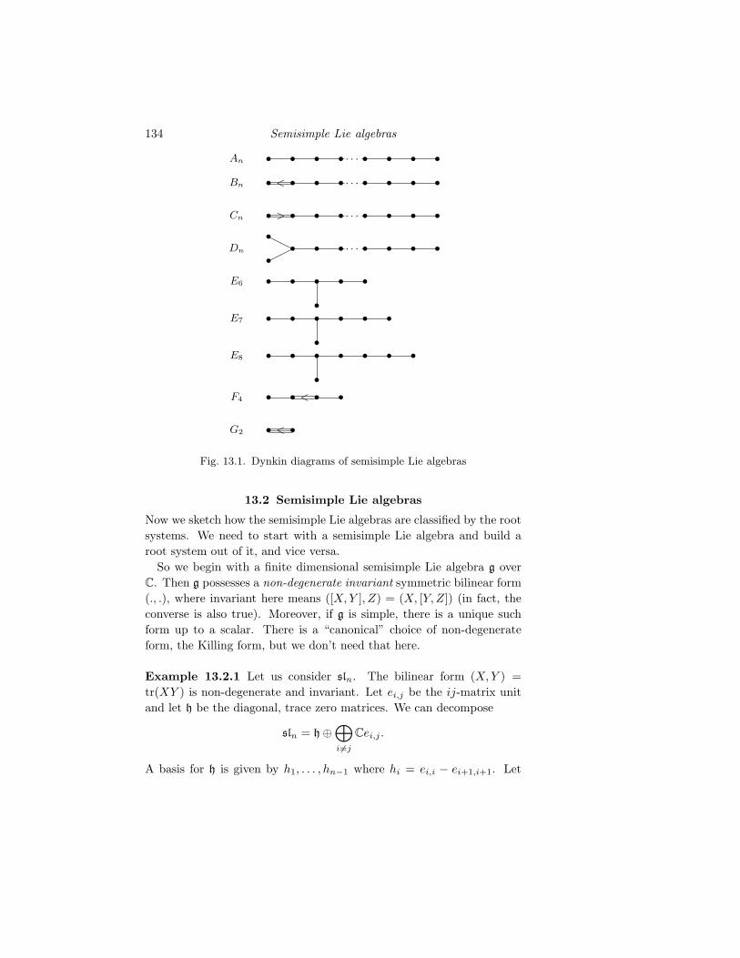
134 Semisimple Lie algebras
An . . .• • • • • • • •
Bn . . .• • • • • • • •<
Cn . . .• • • • • • • •>
Dn . . .H
H• • • • • • ••
•
E6
•
• • • • •
E7
•
• • • • • •
E8
•
• • • • • • •
F4 • • • •<
G2 • •<
Fig. 13.1. Dynkin diagrams of semisimple Lie algebras
13.2 Semisimple Lie algebras
Now we sketch how the semisimple Lie algebras are classified by the rootsystems. We need to start with a semisimple Lie algebra and build aroot system out of it, and vice versa.
So we begin with a finite dimensional semisimple Lie algebra g overC. Then g possesses a non-degenerate invariant symmetric bilinear form(., .), where invariant here means ([X,Y ], Z) = (X, [Y, Z]) (in fact, theconverse is also true). Moreover, if g is simple, there is a unique suchform up to a scalar. There is a “canonical” choice of non-degenerateform, the Killing form, but we don’t need that here.
Example 13.2.1 Let us consider sln. The bilinear form (X,Y ) =tr(XY ) is non-degenerate and invariant. Let ei,j be the ij-matrix unitand let h be the diagonal, trace zero matrices. We can decompose
sln = h⊕⊕i 6=j
Cei,j .
A basis for h is given by h1, . . . , hn−1 where hi = ei,i − ei+1,i+1. Let

13.2 Semisimple Lie algebras 135
εi ∈ h∗ be the map sending a diagonal matrix to its ith diagonal entry.Note ε1 + · · ·+ εn = 0, i.e. the εi’s are not independent. Then for anyH ∈ h we have
[H, ei,j ] = (εi − εj)(H)ei,j ,
i.e. ei,j is a simultaneous eigenvector for h. We use the word weight inplace of eigenvalue, so ei,j is a vector of weight εi − εj . Now you recallthat the root system of type An−1 can be defined as the real vectorsubspace of h∗ spanned by ε1, . . . , εn, and the roots are
Φ := εi − εj | i 6= j.
A base for Φ is given by by α1, . . . , αn−1 where αi = εi − εi+1. Let usfinally write gα := Cei,j if α = εi − εj , i.e. the weight space of g ofweight εi − εj . Then
g = h⊕⊕α∈Φ
gα.
In other words, you “see” the root system of type An−1 when you decom-pose g into weight spaces with respect to the diagonal matrices. Finalnote: the inner product giving the Euclidean space structure is inducedby the non-degenerate form defined to start with. Indeed if you computethe matrix (hi, hj) you get back the Cartan matrix of type An−1.
This example is more or less how things go in general, when youstart with an arbitrary semisimple Lie algebra g, with a non-degenerateinvariant form (., .). The first step is to develop in g a theory of Jordandecompositions. This parallels the Jordan decomposition we proved foralgebraic groups. You call an element X of g semisimple if the linearmap adX : g → g is diagonalizable, and nilpotent if adX is nilpotent.The abstract Jordan decomposition shows that any X ∈ g decomposesuniquely as X = Xs + Xn where Xs ∈ g is semisimple and Xn ∈ g isnilpotent, and [Xs, Xn] = 0.
What is more, if you have a representation of g, i.e. a Lie algebrahomomorphism ρ : g→ gln, it is true that ρ(Xs) = ρ(X)s and ρ(Xn) =ρ(X)n, where the semisimple and nilpotent parts on the right handside are taken just as n× n matrices in gln. Thus, the abstract Jordandecomposition is consistent with all other Jordan decompositions arisingfrom all other representations. In particular, semisimple elements of g
map to diagonalizable matrices under any matrix representation of g.For sln, ei,j is nilpotent for i 6= j, and ei,i − ei,j is semisimple.
Now you introduce the notion of a maximal toral subalgebra or Cartan

136 Semisimple Lie algebras
subalgebra h of g (in general maximal toral subalgebra and Cartan subal-gebra are different notions but they agree for semisimple algebras). Thisis a maximal abelian subalgebra all of whose elements are semisimple.It turns out that in a semisimple Lie algebra, maximal toral subalge-bras are non-zero, and they are all conjugate under automorphisms of g.Now fix one – it doesn’t really matter which, since they are all conjugate.Importantly, the restriction of the invariant form (., .) on g to h is stillnon-degenerate. So we can define a map
h∗ → h
mapping α ∈ h∗ to tα ∈ h, where tα is the unique element satisfying(tα, h) = α(h) for all h ∈ h. Now we can lift the non-degenerate form onh to h∗ by defining (α, β) = (tα, tβ). Thus, h∗ now has a non-degeneratesymmetric bilinear form on it too.
For α ∈ h∗, define
gα = X ∈ g | [H,X] = α(H)X for all H ∈ g.
Clearly, g =⊕
α∈h∗ gα. Set Φ = 0 6= α ∈ h∗ | gα 6= 0. Then you getCartan decomposition of g:
g = h⊕⊕α∈Φ
gα
(it is not obvious that the right hand side is everything...). It turns outwith some work that each of the gα spaces are one-dimensional.
Now you can build a root system out of g: we’ve already constructedthe set Φ. Let E be the real vector subspace of h∗ spanned by Φ. Therestriction of the form on h∗ to E turns out to be real valued only, andmakes E into a Euclidean space. Now:
Theorem 13.2.2 The pair (E,Φ) just built out of g (starting from achoice of h) is a root system. Moreover, the resulting map from semisim-ple Lie algebras to Dynkin diagrams gives a bijection between isomor-phism classes of semisimple Lie algebras and Dynkin diagrams. Thedecomposition of a semisimple Lie algebra as a direct sum of simplescorresponds to the decomposition of the Dynkin diagram into indecom-posable components.
For example, sln is the simple Lie algebra corresponding to the Dynkindiagram An−1.

13.3 Construction of simple Lie algebras 137
13.3 Construction of simple Lie algebras
We now explain how to construct the simply-laced simple Lie algebras.So let (E,Φ) be a root system of type A`, D` or E`, π = α1, . . . , α` bea base and Φ+ the corresponding set of positive roots. We may assumethat (α, α) = 2 for all α ∈ Φ, as all roots have the same length. LetQ = ZΦ ⊂ E be the root lattice, the free abelian group on basis Π.
We construct an asymmetry function
ε : Q×Q→ ±1
such that
(1) ε is bilinear, i.e. ε(α + α′, β) = ε(α, β)ε(α′, β) and ε(α, β + β′) =ε(α, β)ε(α, β′) for all α, α′, β, β′ ∈ Q.
(2) ε(α, α) = (−1)(α,α)/2 for all α ∈ Q.
Note (2) implies
(3) ε(α, β)ε(β, α) = (−1)(α,β) for all α, β ∈ Q.
To construct such an ε, it suffices by bilinearity to define it on elementsof Π. Choose an orientation of the Dynkin diagram. Then define
ε(αi, αj) =
1 if αi and αj are not connected,1 if αi → αj ,−1 if αi ← αj ,−1 if αi = αj .
Now we can construct g. Let h∗ = C ⊗Z Q = C ⊗R E. Let h be thedual space, and let Hα ∈ h be the element such that β(Hα) = (β, α) forall β ∈ h∗. Then, H1, . . . ,H` gives a basis for h, where Hi = Hαi .
Now let
g = h⊕⊕α∈Φ
CEα
as a vector space. Define a multiplication by the formulae
[Hi,Hj ] = 0,
[Hi, Eα] = α(Hi)Eα = (αi, α)Eα,
[Eα, E−α] = −Hα,
[Eα, Eβ ] = 0 if α+ β /∈ ϕ ∪ 0,[Eα, Eβ ] = ε(α, β)Eα+β if α+ β ∈ Φ.

138 Semisimple Lie algebras
Theorem 13.3.1 g is the simple Lie algebra of type Φ, with maximaltoral subalgebra h.
Proof You of course have to check that g is a Lie algebra, which boilsdown to checking that the Jacobi identity is satisfied. This is a caseanalysis.
Having done that, we define a bilinear form on g by
(Hi,Hj) = (αi, αj), (Hi, Eα) = 0, (Eα, Eβ) = −δα,−β .
You check that this is a non-degenerate invariant bilinear form. More-over, h is a toral subalgebra of g, and since the 0-weight space of h ong is just h itself, it must be maximal. Finally, it is automatic that thecorresponding root system is of type Φ. Hence, g is simple of type Φwith maximal toral subalgebra h.
Definition 13.3.2 Let g be an arbitrary semisimple Lie algebra (notnecessarily simply-laced). Let Φ be a root system corresponding to achoice of maximal toral subalgebra h, and let Π = α1, . . . , α` be abase for Φ. For α, β ∈ Φ, the α-string through β is the sequence
β − rα, . . . , β, . . . , β + qα
where r and s are the maximal integers such that all the vectors in thestring belong to Φ. It turns out that r and q are equal to 0, 1, 2 or 3 inall cases, and 2 and 3 don’t arise if the root system is simply-laced.
Denote Hα := 2tα/(α, α) and Hi := Hαi. A Chevalley basis for g
means a basis
H1, . . . ,H` ∪ Xα | α ∈ Φ
such that
(a) [Hi,Hj ] = 0,(b) [Hi, Xα] = (α, α∨i )Xα,(c) [Xα, X−α] = Hα, and this is a Z-linear combination ofH1, . . . ,H`,(d) If α, β, α+ β ∈ Φ and β − rα, . . . , β + qα is the α-string through
β, then [Xα, Xβ ] = Nα,βXα+β = ±(r + 1)Xα+β .
The key thing is that all the structure constants in a Chevalley basis areintegers!
Theorem 13.3.3 (Chevalley) Chevalley bases exist.

13.4 Kostant Z-form 139
Proof If Φ is simply-laced, this is easy from the above construction:take Xα = Eα if α ∈ Φ+ and −Eα is α ∈ Φ−. Now you easily checkthis satisfies the properties. If Φ is not simply-laced, we need someother construction. For classical Lie algebras that is not too hard: youcan write them down just as explicitly as sln. Problem 13.6.4 gives anexample of how you do this. Another way is to realize all the non-simply-laced root systems as fixed points of automorphisms of simple-laced ones.
13.4 Kostant Z-form
Informally speaking, Chevalley group is constructed from a semisimpleLie algebra g as the group generated by the ‘exponents’ of the formexp(tXα) where Xα is a root element of the Lie algebra and t is a scalar.But there are some problems here. Consider, for example
exp(Xα) = 1 +Xα +X2α/2! +X3
α/3! + . . .
What does that mean? We don’t have a toplogy to speak of convergence,so we need to make sure that the sum is finite. Well, this will be achievedif Xα is nilpotent in a certain sense. Further, what does X3
α mean? Wecan’t multiply in a Lie algebra! However we can consider this as anelement of the universal enveloping algebra. There is a further problemhowever. If characteristic is 2 or 3, we can’t make sense of the divisionby 3!. The solution to this is very clever—we will first divide by 3! andthen pass to characteristic p!! More formally, we will consider a Z-formUZ of the universal enveloping algebra U of g which contains all Xn
α/n!and then pass to the algebra U = Uk := UZ⊗Zk, called the hyperalgebra.
First, recall the universal enveloping algebra U(g) associated to a Liealgebra g. It is defined by a universal property, but there is also anexplicit construction. The all-important PBW theorem shows that wecan identify g with a Lie subalgebra of U(g), and moreover if X1, . . . , XN
is a basis for g, then the monomials
Xr11 . . . Xrn
N
give a basis for U(g).One reason U(g) is important is because it allows you to view rep-
resentations, i.e. Lie algebra homomorphisms ρ : g → gl(V ), as U(g)-modules:

140 Semisimple Lie algebras
Lemma 13.4.1 The categories of representations of g and of U(g)-modules are isomorphic.
Proof Let ρ : g→ gl(V ) be a representation. Viewing gl(V ) as End (V ),we get induced a unique associative algebra homomorphism ρ : U(g)→End (V ). Using this, we make V into a U(g)-module by u.v = ρ(u)(v). Ifyou think about it, this gives a functor representations of g → U(g)-modules. Conversely, given a U(g)-module, define ρ : g → gl(V ) byρ(X)(v) := Xv. This defines an inverse functor.
Now we state the main result about the Kostant Z-form.
Theorem 13.4.2 Let g be a semisimple Lie algebra over C, with Cheval-ley basis H1, . . . ,H` ∪ Xα | α ∈ Φ. Let UZ be the Z-subalgebra ofU(g) generated by the Xr
α/r! for all α ∈ Π, r ≥ 1. Then, UZ is free as aZ-module with basis given by all monomials in the
Xrαα /|rα! (α ∈ Φ),
(Hi
mi
)(i = 1, . . . , `)
in some fixed order, where mi, rα ≥ 0.
Proof (1) Observe all the “Kostant monomials” form a C-basis for U(g)by the PBW theorem, so they are linearly independent.
(2) Observe all X(r)α and all
(Hi
mi
)belong to UZ – by constructing
them as various commutators of the generators of UZ. Hence all Kostantmonomials belong to UZ.
(3) Prove that the product of two Kostant monomials can be expandedas a Z-linear combination of other Kostant monomials. Hence they spanUZ. This is done by proving various commutation relations.
13.5 Weights and representations
Let Q = ZΦ ⊂ h∗ be the root lattice. Let P be the weight lattice, definedas
P = λ ∈ h∗ | λ(Hi) ∈ Z for all i = 1, . . . , `.
Thus P is the lattice dual to the lattice ZH1+ · · ·+ZH` in h. Obviously,Q ⊆ P . Moreover, since P and Q are both lattices in h∗, i.e. they areboth finitely generated abelian groups that span h∗ over C, the quotient

13.5 Weights and representations 141
P/Q is a finitely generated, torsion abelian group. But that implies P/Qis a finite abelian group. It is called the fundamental group.
To get a basis for P (as a free abelian group), one can take the fun-damental weights ω1, . . . , ω` defined by
ωi(Hj) = δi,j ,
i.e. the dual basis to H1, . . . ,H`. We claim that
αi =∑j=1
ai,jωj
where ai,j = (αi, α∨j ) = αi(Hj) is the Cartan integer. To see this, justevaluate both sides on Hj – you get the same thing. Thus, P/Q is theabelian group on generators ω1, . . . , ωj subject to relations
∑j=1
ai,jωj = 0.
Considering elementary divisors, you get that
|P/Q| = detA,
indeed, you get an explicit description of P/Q as an abelian group.These are the orders:
A` : `+ 1
B`, C`, E7 : 2
D` : 4
E6 : 3
E8, F4, G2 : 1
In fact the fundamental group is cyclic in all cases except for D` with `even, when it is Z/2×Z/2. This is going to be very important: we nowknow exactly all possible lattices lying between Q and P .
The last important ingredient that we need to construct the Chevalleygroups is a little representation theory of semisimple Lie algebras. Weare interested here just in the finite dimensional representations of g. Afundamental theorem of Weyl (mentioned before) shows that any finitedimensional representation of g decomposes as a direct sum of irrduciblerepresentations, i.e. ones with no proper invariant submodules. So wereally only need to discuss the finite dimensional irreducible representa-tions.

142 Semisimple Lie algebras
Now, if V is a finite dimensional U(g)-module, we can decompose
V =⊕λ∈h∗
Vλ
where
Vλ = v ∈ V |Hv = λ(H)v for all H ∈ h.
This is the weight space decomposition of V . For example, the Cartandecomposition of g itself is the weight space decomposition of the adjointrepresentation. We will say that v ∈ V is a high weight vector of highweight λ if 0 6= v ∈ Vλ and Xαv = 0 for all α ∈ Φ+. It is obvious thatany non-zero finite dimensional V possesses such a vector – becauseXαVλ ⊆ Vλ+α and there are only finitely many non-zero weight spacesin total.
It turns out that the high weight vector of an irreducible representa-tion of g is unique up to a scalar and its weight belongs to the set
P+ = λ ∈ P | λ(Hi) ≥ 0 for each i = 1, . . . , `.
Conversely, for any element of P+, there is a unique up to isomorphismirreducible representation of that highest weight.
Relation to Z-forms is as follows:
Theorem 13.5.1 Let λ ∈ P+ and V be the corresponding irreduciblehighest weight representation. Then, there exists a lattice VZ in V in-variant under the action of the Kostant Z-form UZ, such that
VZ =∑µ∈h∗
Vµ,Z
where Vµ,Z = Vµ ∩ VZ.
Given any finite dimensional representation V , we consider its latticeL(V ), which is defined to be the subgroup of P generated by all λ suchthat Vλ 6= 0. If V is faithful, then Q ⊆ L(V ) ⊆ P . In fact you can getany intermediate lattice arising for suitable choice of V , and the possiblelattices are parametrized by the subgroups of the fundamental group.
13.6 Problems
Problem 13.6.1 Write down the explicit construction of the root sys-tems of type A`, B`, C` and D`, and show that the length of the longest

13.6 Problems 143
element w0 of the Weyl group was `(`+1)/2. (Hint: You need to look itup! There are many good sources, e.g. Humphreys’ “Introduction to Liealgebras and representation theory”, Bourbaki “Groupes et Algebres deLie”, Kac “Infinite dimensional Lie algebras”, Carter “Finite groups ofLie type”, Helgason “Differential geometry and symmetric spaces”...)
Problem 13.6.2 Look up or work out the dimensions of the simple Liealgebras of types A`, B`, C` and D`. In particular, check that dimC` isthe same as the dimension of the algebraic group Sp2`.
Problem 13.6.3 In the proof of Theorem 13.3.1, go through the detailsneeded to verify that the bilinear form defined is invariant.
Problem 13.6.4 Let V be a (2`+1)-dimensional complex vector spacewith an ordered basis e1, . . . , e`, e0, e−`, . . . , e−1. Define a symmetricbilinear form on V by declaring (ei, ej) = 0 (i 6= −j), (ei, e−i) = 1(i 6= 0) and (e0, e0) = 2. Let J be the matrix of this bilinear form in thebasis, ordering rows and columns as e1, . . . , e`, e0, e−`, . . . , e−1.
(i) Compute the matrix J explicitly.
(ii) Let g = X ∈ gl(V ) |XTJ + JX = 0 be the Lie algebra so(V ) =so(2`+1). Viewing elements of g as block matrices in our ordered basis,we can write
X =
A v B
r x s
C w D
.
Compute explicitly the conditions that the `×` matrices A,B,C,D, thecolumn vectors v, w, the row vectors r, s and the scalar x must satisfyfor X to belong to g.
(iii) Let h be the set of all diagonal matrices in g. This is a toralsubalgebra of g. Let εi ∈ h∗ be the function
diag(t1, . . . , t`, 0,−t`, . . . ,−t1) 7→ ti,
so that ε1, . . . , ε` form a basis for h∗. Let
Φ = ±εi ± εj ,±εk | 1 ≤ i < j ≤ `, 1 ≤ k ≤ `,
the root system of type B`. Let Ei,j : V → V denote the linear map

144 Semisimple Lie algebras
with Ei,j .vk = δjkvi for all −` ≤ i, j, k ≤ `. For α ∈ Φ, define
α εi − εj(i < j) εi + εj(i < j) εiXα Ei,j − E−j,−i Ej,−i − Ei,−j 2Ei,0 − E0,−i
X−α Ej,i − E−i,−j E−i,j − E−j,i E0,i − 2E−i,0
Verify that
g = h⊕⊕α∈Φ
CXα
is the Cartan decomposition of g.(v) DefiningH1, . . . ,H` appropriately, check that H1, . . . ,H`∪Xα|α ∈
Φ is a Chevalley basis for g.

14
The Chevalley construction
To motivate the construction, let’s stick to working over C for a bit. Letg be a semisimple Lie algebra, and let V be a finite dimensional faithfulrepresentation. So the lattice L(V ) is some intermediate lattice betweenQ and P (e.g. if V is the adjoint representation, L(V ) = Q).
Let Hi ∪ Xα be a Chevalley basis. Since V has only finitelymany weight spaces and the Xα map Vµ into Vµ+α, each Xα acts on Vnilpotently. Thus, we can consider the formal series
exp(cXα) = 1 + cXα + c2X2α/2! + . . .
for any scalar c ∈ C as a well-defined endomorphism of V (the infinitesum terminates...).
By familiar properties of exponential series,
exp(cXα) exp(dXα) = exp((c+ d)Xα).
In particular, exp(cXα) is invertible with inverse exp(−cXα). Now letG be the subgroup of GL(V ) generated by all exp(cXα) for all c ∈ Cand α ∈ Φ. This is the Chevalley group corresponding to g in therepresentation V . It turns out that (up to isomorphism) G is determinedby g and the lattice L(V ).
Using Z-forms we can imitate this construction over an arbitrary fieldk. In the case that k is an algebraically closed field, G is always asemisimple algebraic group, and in fact all semisimple algebraic groupsarise out of this contstruction for some choice of Φ and L(V ).
In order to study the structure of G in detail, we construct closedsubgroups U, T,B,N of G with explicitly named generators, and provevarious relations between these generators. We will show that B = UoT(semidirect product), that T N , and identify the quotient group N/Twith the original Weyl group W .
145

146 The Chevalley construction
Finally, we will prove the Bruhat decomposition:
G =⋃w∈W
BwB.
Here w ∈ W needs to be interpreted as a fixed coset representative inN . Thus, the (B,B)-double cosets in G are parametrized by the Weylgroup W .
14.1 Definition and first properties
To every field, every root system Φ and every lattice L such that Q ⊆L ⊆ P we associate the Chevalley group G = G(k,Φ, L) defined as fol-lows. Let UZ be the Kostant Z-form of the universal enveloping algebraU(g) of the semisimple Lie algebra g of type Φ, and VC be a represen-tation of g with L = L(V ). Pick a UZ-invariant lattice VZ in V as inTheorem 13.5.1. Let V = VZ ⊗Z k. Then for any t ∈ k and α ∈ Φ,
xα(t) := exp(tXα) = 1 +Xα ⊗ t+ (X2α/2!)⊗ t2 + . . .
can be considered as an invertible endomorphism of V . By definition, Gis the group generated by all xα(t) for t ∈ k and α ∈ Φ.
The proof that the group only depends on L and not on the choice ofVC and VZ ⊂ VC will be skipped.
For fixed α ∈ Φ, let Xα be the subgroup of GL(V ) generated by allxα(t) for all t ∈ k.
From now on we assume as usual that k is algebraically closed.
Theorem 14.1.1 The group G is a closed connected subgroup of GL(V ).
Proof Note that the map Ga → GL(V ), t 7→ xα(t) is a morphism ofalgebraic groups, as the exponent stops after finitely many steps andso is ”polynomial” in t. So each Xα is a closed connected subgroup ofGL(V ). Now use Corollary 8.2.7.
The main goal of this course is to prove that: (a) G is a semisimplealgebraic group and (b) every semisimple algebraic group is obtained inthis way. You have probably already figured out that we are not goingto get there by the end of the term but we will try to get as far aspossible...
Concerning (a), it is a well known fact (often proved even in the 600algebra courses) that PSLn(k) is simple as an abstract group (all youneed for this is the assumption that k has more than 3 elements if n = 2,

14.1 Definition and first properties 147
but remember that for us k is algebraically closed, so infinite). So if Gis of type A, any of its solvable normal subgroups is contained in thecenter of G, which is finite. As the radical is connected, this proves thatthe radical of G is trivial. The proof for other types uses elements xα(t)instead of transvections in the usual proof for PSLn, and we will notreproduce it here.
15
Borel subgroups and flag varieties
In the previous chapter, we sketched the construction of the semisimplealgebraic groups. It is very explicit and case-free. We will now go back toalgebraic geometry and sketch the proof of the Classification Theorem.We will see that algebraic geometry, in particular the variety structureon quotient varieties G/H which we haven’t really used yet in a deepway, is a fundamental tool to studying group theory.
15.1 Complete varieties and Borel’s fixed point theorem
Recall the notion of the complete variety from chapter 7. We need thefollowing:
Lemma 15.1.1 Let G be an algebraic group acting transitively on va-rieties X,Y . Let ϕ : X → Y be a bijective, G-equivariant morphism. IfY is complete, then X is complete.
Proof By Remark 7.1.3(ii), we need to show that π2 : X × Z → Z
is closed for all affine varieties Z. Since Y is complete, it suffices toprove that ϕ × id : X × Z → Y × Z is closed. By Proposition 5.3.2,there are open subsets U ⊂ X and V ⊂ Y such that ϕ(U) = V andϕ|U : U → V is a finite morphism. Let R,S, T be the respective affinealgebras of U, V, Z. Since R is integral over S, R ⊗ T is integral overS ⊗ T . Therefore ϕ × id : U × Z → V × Z is also a finite morphism.In particular, it is a closed map, see Corollary 5.2.4. Because G actstransitively on X, Y and ϕ is G-equivariant, X (resp. Y ) is covered byfinitely many translates of the form xU (resp. xV ) for some x ∈ G. Itfollows that ϕ× id : X × Z → Y × Z is closed.
148

15.2 Borel subgroups 149
Now we can prove the important
Theorem 15.1.2 (Borel’s fixed point theorem) Let G be a con-nected solvable algebraic group, and X be a non-empty complete G-variety. Then G has a fixed point on X.
Proof Proceed by induction on dimG, the case G = 1 being trivial.Suppose then that dimG > 0 and let H = G′, which is connectedsolvable of strictly smaller dimension. By induction,
Y = x ∈ X |Hx = x
is non-empty. By Lemma 8.3.1(iii), Y is closed, hence complete, and Gstabilizes Y as H G. So we may as well replace X by Y to assumethat H ⊆ Gx for all x ∈ X. Since G/H is abelian, this implies that eachGx G.
Now choose x so that the orbit G · x is of minimal dimension. Then,G · x is closed hence complete. The map G/Gx → G.x is bijective, sowe deduce that G/Gx is complete by the preceeding lemma. But G/Gxis affine as Gx G. So in fact G/Gx is a point, i.e. G = Gx and x is afixed point.
Corollary 15.1.3 (Lie-Kolchin theorem) Let G be a connected solv-able subgroup of GL(V ). Then G fixes a flag in V .
Proof Let G act on the flag variety F(V ). This is projective, so G hasa fixed point.
15.2 Borel subgroups
Let G be a connected algebraic group.
Definition 15.2.1 A Borel subgroup B of G is a maximal closed con-nected solvable subgroup of G.
Example 15.2.2 (i) If G is a Chevalley group, the subgroup B = TU isa Borel subgroup of G. Any conjugate of B in G will give another suchsubgroup.
(ii) If G = GLn, the subgroup B of all upper triangular matricesis a maximal closed connected solvable subgroup by the Lie-Kolchintheorem. Hence, it is a Borel subgroup. Any conjugate of this will give

150 Borel subgroups and flag varieties
another. Note in this case that the quotient variety G/B is the flagvariety, so it is a projective variety in particular.
Theorem 15.2.3 For any connected algebraic group G, let B be a Borelsubgroup. Then, G/B is a projective variety, and all other Borel sub-groups of G are conjugate to B.
Proof Let S be a a Borel subgroup of maximal dimension. Apply Cheval-ley’s theorem to construct a representation ρ : G→ GL(V ) and a 1-spaceL ⊂ V such that S = StabG(L). By the Lie-Kolchin theorem, S fixes aflag in V/L. Hence S fixes a flag F = (L = L1 ⊂ L2 ⊂ · · · ⊂ Ln = V )in the flag variety F(V ). Recall this is a projective variety, hence it iscomplete.
By the choice of L, S = StabG(F ). Hence the orbit map induces abijective morphism G/S → G · F ⊂ F(V ). Take any other flag F ′ ∈F(V ). Then StabG(F ′) is upper triangular in some basis, hence it issolvable, hence its dimension is ≤ dimS. This shows that dimG · F ′ =dimG − dim StabG(F ′) ≥ dimG · F . Therefore, G · F is a G-orbit inF(V ) of minimal dimension, hence it is closed. This shows that G · Fis also complete, so G/S is complete too. Now G/S is complete and itsquasi-projective, hence it is projective.
Finally, let B be another Borel subgroup of G. Then B acts on G/S,so by Borel’s fixed point theorem, B has a fixed point gS on G/S.Therefore BgS = gS, i.e. g−1Bg ⊆ S. By maximality, we get thatg−1Bg = S and this completes the proof.
Definition 15.2.4 A parabolic subgroup P of G is any closed subgroupof G such that G/P is a projective (equivalently, complete) variety.
Theorem 15.2.5 Let P be a closed subgroup of G. Then, P is parabolicif and only if it contains a Borel subgroup. In particular, P is a Borelsubgroup if and only if P is connected solvable and G/P is a projectivevariety.
Proof Suppose G/P is projective. Let B be a Borel subgroup of G.It acts on G/P with a fixed point, say BgP = gP . This implies thatg−1Bg ⊆ P , i.e. P contains a Borel subgroup.
Conversely, suppose P contains a Borel subgroup B. The map G/B →G/P is surjective and G/B is complete. Hence, G/P is complete too.But it is quasi-projective too, so in fact G/P is projective.

15.3 The Bruhat order 151
Example 15.2.6 (i) Let G = GLn. The subgroups of G containing B(upper triangular matrices) are exactly the “step” subgroups, one foreach way of writing n = n1 + · · · + ns as a sum of positive integersn1, . . . , ns. There are 2n−1 such subgroups.
(ii) Let G be an arbitrary Chevalley group. Let S be a subset ofthe simple roots Π, so there are 2` possibilities for S. Let P be thesubgroup of G generated by B and all sα for α ∈ S. (Equivalently, P isthe subgroup generated by T and the Xα’s for α ∈ Φ+ ∪ (−S).) Then,P contains B so it is a parabolic subgroup by the theorem, and G/P isa projective variety. In fact, these P ’s give all the parabolic subgroupsof G containing the fixed choice of Borel subgroup B. By the theorem,all other parabolic subgroups of G are conjugate to one of these. Thereare exactly 2` different conjugacy classes of parabolic subgroup in theChevalley group G.
15.3 The Bruhat order
Let G be a Chevalley group, with all the subgroups U, T,Xα, B,N,W =N/T ,. . . . Recall also that W is generated by the simple reflectionssα | α ∈ Π. For any w ∈ W , we can write w as a product of simplereflections. The length of w was the length of a shortest such expression,called a reduced expression for W .
Let me define a partial order on W as follows. Take w,w′ ∈ W . Letw = s1 . . . sr be a reduced expression for w. Declare that w′ ≤ w ifand only if w′ = si1 . . . sij for some 1 ≤ i1 < · · · < ij ≤ r, i.e. if w′
is a “subexpression” of w. How do you prove this really is a partialorder? How do you even show that it is well-defined, i.e. independentof the choice of the reduced expression of w? One of the ways is to usealgebraic geometry!
By the Bruhat decomposition, the B-orbits on G/B are parametrizedby the Weyl groupW , i.e. the orbits are the BwB/B’s. Now, the closureof an orbit is a union of orbits, the ones in the boundary being of strictlysmaller dimension. So there is obviously a partial ordering ≤ on theorbits of B on G/B defined by O ≤ O′ if and only if O ⊆ O′. Whatwe are going to prove is that this is exactly the partial ordering definedin the previous paragraph! In other words, the ordering in the previousparagraph IS well-defined because there is a geometrically defined partialordering that amounts to the combinatorics there.
Let’s proceed with some lemmas.

152 Borel subgroups and flag varieties
Lemma 15.3.1 Let G be an algebraic group, X a G-variety, H ≤ G aclosed subgroup and Y ⊆ X a closed H-stable subvariety of X. If G/His a complete variety (i.e. if H is a parabolic subgroup of G) then G · Yis closed in X.
Proof Let A = (g, x) ∈ G×X | g−1x ∈ Y , which is closed in G×X.Let
π : G×X → G/H ×X
be the quotient map. Recall this is an open map. If (g, x) ∈ A then(gh, x) ∈ A for all h ∈ H, since H stabilizes Y . Hence,
π(A) = G/H ×X − π(G×X −A),
so π(A) is closed in G/H ×X. Since G/H is complete, the projectionprX(π(A)) ⊆ X is also closed. This is exactly G · Y .
Lemma 15.3.2 Any product of parabolic subgroups of G containing Bis closed in G.
Proof Let P1, . . . , Pr be parabolic subgroups of G containing B. Byinduction, P2 . . . Pr is closed in G and B-stable. Note P2 . . . Pr.B =P1 . . . Pr−1 is closed and B-stable. Since P1/B is complete, we get bythe lemma that P1P2 . . . Pr is closed too.
Theorem 15.3.3 (Chevalley) Let G be a Chevalley group. Fix w ∈Wand a reduced expression w = s1 . . . sr for w as a product of simplereflections. Then,
BwB =⋃w′
Bw′B
where w′ runs over all subexpressions si1 . . . sij of s1 . . . sr.
Proof Let w = s1 . . . sr be the fixed reduced expression for w, Let
Pi = 〈B, si〉 = B ∪BsiB,
where the last equality comes from the work on Chevalley groups in theprevious chapter. We show by induction on r that
P1 . . . Pr =⋃w′
Bw′B

15.3 The Bruhat order 153
where the union is taken over all subexpressions w′ of the reduced ex-pression s1 . . . sr. The case r = 1 is already done!
Now suppose r > 1. Then by induction,
P1 . . . Pr =⋃w′′
Bw′′B.(B ∪BsrB)
where w′′ runs over all subexpressions of s1 . . . sr−1. But that equals⋃w′
Bw′B
as required, since Bw′′srB ⊆ Bw′′BBsrB ⊆ Bw′′B ∪ Bw′′srB by the
previous chapter.By the preceeding lemma, P1 . . . Pr is closed, hence⋃
w′
Bw′B,
union over all subexpressions w′ of s1 . . . sr, is closed. So it certainly con-tains the closure BwB. Finally, we know dimBwB is equal to dimB+the number of positive roots sent to negative roots by w. So in fact wemust have that ⋃
w′
Bw′B = BwB
by dimension.
Now since BwB is defined intrinsically independent of any choice ofreduced expression of w, the relation w′ ≤ w iff w′ is a subexpressionof some fixed reduced expression for w is well-defined independent ofthe choice. Moreover, it is a partial ordering on W called the Bruhatordering.
For w ∈W , the Schubert variety
Xw := BwB/B
is a closed subvariety of the flag variety G/B. Note Xw is no longer anorbit of an algebraic group, so it needn’t be smooth. Schubert varietiesare extremely interesting projective varieties with many wonderful prop-erties. The Schubert variety Xw0 is the flag variety itself, the Schubertvariety X1 is a point. We have shown above that in general, the latticeof containments of Schubert varieties is isomorphic to the Bruhat orderon W .

16
The classification of reductive algebraicgroups
16.1 Maximal tori and the root system
Now we sketch the procedure to build a root system starting from anarbitrary reductive algebraic group. This is the first step in proving theclassiciation of reductive algebraic groups.
Let us start by talking about tori. Recall an n-dimensional torus is analgebraic group isomorphic to Gm×· · ·×Gm. For example, the subgroupDn of GLn consisting of all diagonal matrices is an n dimensional torus.Let T be an n-dimensional torus. The character group
X(T ) = Hom(T,Gm) ∼= Hom(Gm,Gm)⊕n ∼= Zn.
An important point is that, given any two tori T and T ′,
Hom(T, T ′) ∼= Hom(X(T ′), X(T )).
So any homomorphism f : X(T ′) → X(T ) of abelian groups induces aunique morphism T → T ′ of algebraic groups, and vice versa. In fact,you can view X(?) as a contravariant equivalence of categories betweenthe category of tori and the category of finitely generated free abeliangroups.
All elements of a torus T are semisimple. So if V is any finite di-mensional representation of T , every element of T is diagonalizable inits action on V by the Jordan decomposition. Moreover, they commute,hence we can actually diagonalize
V =⊕
λ∈X(T )
Vλ
where
Vλ = v ∈ V | tv = λ(t)v for all t ∈ T.
154

16.1 Maximal tori and the root system 155
As before, the Vλ’s are called the weight spaces of V with respect to thetorus T .
Now let G be an arbitrary connected algebraic group. A maximaltorus of G is what you’d think: a closed subgroup T that is maximalsubject to being a torus. Let me state some theorems about maximaltori in connected solvable groups. These are proved by induction, thoughit is often quite difficult...
Theorem 16.1.1 Let G be a connected solvable group. Then, the setGu of all unipotent elements of G is a closed connected normal subgroupof G. All the maximal tori of G are conjugate, and if T is any one ofthem, then G is the semi-direct product of T acting on Gu.
As a consequence, you show that in an arbitrary connected group G,all its maximal tori are conjugate. Indeed, any maximal torus T of Gis contained in a Borel subgroup B. If T ′ is another maximal torus,contained in a Borel B′, we can conjugate B′ to B to assume that T ′
is also contained in B. But then T and T ′ are conjugate in B by thetheorem.
Now start to assume that G is a reductive algebraic group. Let Tbe a maximal torus. Let g be the Lie algebra of G. We can view g asa representation of T via the adjoint action. It turns out moreover –using for the first time that G is reductive – that the zero weight spaceof g with respect to T is exactly the Lie algebra t of T itself. So we candecompose
g = t⊕⊕α∈Φ
gα
where Φ is the set of all 0 6= α ∈ X(T ) such that the T -weight spacegα 6= 0. You can already see the root system emerging... The differencenow however is that the set Φ of roots is a subset of the free abeliangroup X(T ). Now using the assumption that G is reductive again, youshow:
(1) Each gα is one dimensional, and α ∈ Φ iff −α ∈ Φ.(2) The group W = NG(T )/T is a finite group that acts naturally on
X(T ) and permutes the subset Φ ⊆ X(T ).(3) Let Q be the root lattice, the subgroup of X(T ) generated by Φ, and
let E = R ⊗Z Q. Fix a positive definite inner product on E that isinvariant under the action of W . Then, (E,Φ) is an abstract rootsystem.

156 The classification of reductive algebraic groups
(4) If we embed T into a Borel subgroup B, we get a choice Φ+ of positiveroots defined by α ∈ Φ+ iff gα ⊂ b. Conversely, any choice Φ+ ofpositive roots determines a unique Borel subgroup of G containing T .
We’ve now built out of G a root system (E,Φ), and realized the Weylgroup W explicitly as the quotient group NG(T )/T . Moreover, Φ is asubset of the character group X(T ) of T .
If G is semisimple, then G is determined up to isomorphism by itsroot system (E,Φ) together with the extra information given by thefundamental group X(T )/Q. In the next section, we will see a morenatural setup which classifies the reductive, not just semisimple, groups.This is harder, since X(T ) will in general be of bigger rank than Q, andso there is much more freedom not captured by the fundamental groupalone. For GLn, X(T ) is a free abelian group of rank n, whereas Q is ofrank (n− 1).
16.2 Sketch of the classification
Finally let’s prepare the way to state the classification of reductive al-gebraic groups in general. Let G be a reductive algebraic group, and letT be a maximal torus. Let Φ ⊂ X(T ) be the root system of G, definedfrom the decomposition
g = t⊕⊕α∈Φ
gα.
Let
X(T ) = Hom(T,Gm)
be the character group of T , and let
Y (T ) = Hom(Gm, T )
be the cocharacter group. This is also a free abelian group of rank dimT .Moreover, there is a pairing
X(T )× Y (T )→ Z
defined as follows. Given λ ∈ X(T ) and ϕ ∈ Y (T ), the composite λ ϕis a map Gm → Gm. So since Aut(Gm) = Z,
(λ ϕ)(x) = x〈λ,ϕ〉
for a unique 〈λ, ϕ〉 ∈ Z.

16.2 Sketch of the classification 157
For each α ∈ Φ, you prove that there is a (unique up to scalars)homomorphism
xα : Ga → G
such that
txα(c)t−1 = xα(α(t)c)
for all c ∈ Ga, t ∈ T , such that the tangent map
dxα : L(Ga)→ gα
is an isomorphism. Moreover, the xα’s can be normalized so that thereis a homomorphism
ϕα : SL2 → G
such that
ϕα
(1 c
0 1
)= xα(c), ϕα
(1 0c 1
)= x−α(c).
Define
α∨ : Gm → T, α∨(c) = ϕα
(c 00 c−1
).
So α∨ ∈ Y (T ). This is called the coroot associated to the root α ∈ Φ.Now we have built a datum (X(T ),Φ, Y (T ),Φ∨), where Φ∨ is the set
of all coroots. This is the root datum of G with respect to the torus T .(Actually, since all maximal tori in G are conjugate, it doesn’t dependup to isomorphism on the choice of T .) The notion of root datum isthe appropriate generalization of root system to take care of arbitraryreductive algebraic groups, not just the semisimple ones.
Here is an axiomatic formulation of the notion of root datum: a rootdatum is a quadruple (X,Φ, Y,Φ∨) where
(a) X (“characters”) and Y (“cocharacters”) are free abelian groups offinite rank, in duality by a pairing 〈., .〉 : X × Y → Z;
(b) Φ ⊂ X (“roots”) and Φ∨ ⊂ Y (“coroots”) are finite subsets, and thereis a given bijection α 7→ α∨ from Φ to Φ∨.
To record the additional axioms, define for α ∈ Φ the endomorphismssα, s
∨α of X,Y respectively by
sα(x) = x− 〈x, α∨〉α, s∨α(y) = y − 〈α, y〉α∨.
Then we have the axioms:

158 The classification of reductive algebraic groups
(RD1) For α ∈ Φ, 〈α, α∨〉 = 2.(RD2) For α ∈ Φ, sαΦ = Φ, s∨αΦ∨ = Φ∨.
The datum (X(T ),Φ, Y (T ),Φ∨) built from our algebraic group G earlieris such a gadget.
There is a notion of morphism of root datum
(X,Φ, Y,Φ∨)→ (X ′,Φ′, Y ′, (Φ′)∨) :
a map f : X ′ → X that maps Φ′ bijectively onto Φ and such that thedual map f∨ : Y → Y ′ maps f(α)∨ to α∨ for all α ∈ Φ′. Hence there isa notion of isomorphism of root datums.
Now suppose that G,G′ are reductive algebraic groups with maximaltori T, T ′ respectively and corresponding root data (X(T ),Φ, Y (T ),Φ∨)and the primed version. Let f : (X(T ), . . . ) → (X ′(T ), . . . ) be a mor-phism of root data. It induces a dual map f : T → T ′ of tori. The stepis to show that f can be extended to a homomorphism f : G→ G′.
Using it you prove in particular the isomorphism theorem:
Theorem 16.2.1 Two reductive algebraic groups G,G′ are isomorphicif and only if their root datums (relative to some maximal tori) areisomorphic.
There is also an existence theorem:
Theorem 16.2.2 For every root datum, there exists a correspondingreductive algebraic group G.
Finally, one intriguing thing: given a root datum (X,Φ, Y,Φ∨) thereis the dual root datum (Y,Φ∨, X,Φ). If G is a reductive algebraic groupwith root datum (X,Φ, Y,Φ∨) you see there is a dual group G∨ with thecorresponding dual root datum. Note the process of going from G toG∨ is very clumsy: I don’t think there is any direct way of constructingthe dual group out of the original.
Example 16.2.3 Suppose that G is a semisimple algebraic group. LetQ = ZΦ ⊂ X(T ). Here, Q andX(T ) have the same rank, soQ is a latticein X(T ), and X(T )/Q is a finite group, the fundamental group. Let Pbe the dual lattice to Q. Fixing a positive definite W -invariant innerproduct on E = R⊗ZQ, we can identify P with the weight lattice of theroot system of G, and then everything is determined by the relationshipbetween Q ⊆ X(T ) ⊆ P . You can formulate the classification just ofthe semisimple algebraic groups in these terms.

16.2 Sketch of the classification 159
Example 16.2.4 Let G be a semisimple algebraic group, and supposethat Q ⊆ X(T ) ⊆ P are as in the previous example. If X(T ) = P , thenG is called the simply-connected group of type Φ. If X(T ) = Q, thenG is called the adjoint group of this type. Now let Gsc be the simply-connected one, Gad be the adjoint one. Let G be any other semisimplegroup of type Φ. Then, there is an inclusion X(T ) → P = X(Tsc). Thisinduces a map Gsc G. Similarly, there is always a map G Gad.
Example 16.2.5
(1) Consider the root datum of GL2. Here, X(T ) has basis ε1, ε2,these being the characters picking out the diagonal entries. More-over, the positive root is α = ε1−ε2. Also Y (T ) has basis ε∨1 , ε
∨2 ,
the dual basis, mapping Gm into each of the diagonal slots. Thecoroot is α∨ = ε∨1 − ε∨2 .
(2) GL2 is its own dual group.(3) Consider the root datum of SL2 × Gm. Here, X(T ) has basis
α/2, ε, Y (T ) has the dual basis α∨, ε∨ (here α is the usual positiveroot of SL2).
(4) Consider the root datum of PSL2 × Gm. Here, X(T ) has basisα, ε, Y (T ) has the dual basis α∨/2, ε. So PSL2×Gm is the dualgroup to SL2 ×Gm.
(5) As an exercise in applying the classification, you can show that(1),(3) and (4) plus one more, the 4 dimensional torus, are all thereductive algebraic groups of dimension 4.
Example 16.2.6 Here are some more examples of dual groups (I think!).The dual group to SLn is PSLn. The dual group to Sp2n is SO2n+1.The dual group to PSp2n is Spin2n+1. The dual group to SO2n is SO2n.The dual group to Spin2n is PSO2n.
For more explicit constructions of root datums, see Springer, 7.4.7.

Bibliography
[Br] J. Brundan, Lecture Notes on Algebraic Groups.[Hu] J. Humphreys, Linear Algebraic Groups.[Ma] H. Matsumura, Commutative Algebra.[Sh] I.R. Shafarevich, Basic Algebraic Geometry.[Sp] T.A. Springer, Linear Algebraic Groups.[St] R. Steinberg, Lectures on Chevalley Groups.
160