32

Lectures 5-6

Quantum Mechanics is constructed from a set of postulates about the way

microscopic particles behave. These postulates have the same logical role in Quantum

Mechanics that axioms do in Mathematics, or laws do in Thermodynamics. Each of these

– postulates, axioms, and laws – act as the logical foundation on which the theory is built.

They have different origins, and lead to systems with different bases for truth.

Axioms are invented, and then the mathematical system is inferred from them. The only

basis for truth in mathematics is internal consistency based on logical inferences – i.e.

whether a theorem based on the axioms is proven to be correct. There is no basis for

deciding on the truth or falsehood of an axiom however, just for the conclusions from the

axioms.

Laws are summaries of experiments, and some of them are used to develop

complex theoretical systems, as in the case of Thermodynamics. Unlike axioms, the laws

themselves can be proven true or false. There are two bases for this – first, refined

experiments may directly demonstrate that the laws are untrue. Second, experiments can

demonstrate that logically correct predictions based on the laws are untrue, which

logically shows that the laws themselves are untrue. Thus scientific systems differ from

mathematical systems in that internal consistency is no longer sufficient to determine

truth or falsehood – successful comparison to an external reality – experimentation – is

also necessary.

Postulates are similar to axioms in that they are invented by the theorist. They are

different from axioms in that they are invented for the purpose of explaining

experimental observations. The postulates themselves are often not directly testable,

33

however. They are used to develop a theoretical framework – i.e. to make predictions.

These predictions are then compared to experiment. The truth or falsehood of the

postulates is then based on the success or failure of the predictions.

It is important to understand this, because a common trap for students first

encountering Quantum Mechanics is to try to understand the direct justification for the

postulates. This is not possible, since they are not based on direct experience (are not

laws), and most certainly are not based on common sense. Remember that common

sense is based on the direct experience of our senses (hence the name), and the realm of

quantum mechanics is in dimensions of size, energy and mass that are too small to be

detected by our senses. Thus it is pointless to try to understand where the postulates

come from. It is only useful to understand their implications, the way that predictions are

based on them, and the truth or falsehood of these predictions.

The first of the postulates of quantum mechanics is that the wavefunction ψ(x)

contains all available information about the system. If the information is not

contained in ψ(x), then it is information that quantum mechanics says we cannot obtain.

There are two types of wavefunctions. One type of wavefunction is a

wavefunction that is a solution to the Schrödinger equation. These wavefunctions are

called eigenfunctions, and have special properties that we will discuss later. The other

type of wavefunction is a wavefunction that is not a solution to the Schrödinger equation.

In either case, the wavefunction provides a complete description of the measurable

properties of a system. However, in each case, once we’ve determined the wavefunction

that describes a system, we need to learn how to extract the information it contains.

34

As we have seen, one of the bits of information we can obtain is the energy of our

system. We will find that in many cases the solution of the Schrödinger equation yields

only certain discontinuous values of the total energy E. In the cases where E is restricted

to discontinuous values we say that it is quantized. Our first two examples of solving

the Schrödinger equation will include one case where the energies are quantized and one

where they are not.

Let’s return to the Schrödinger equation. If we factor out the ψ(x)'s in our

Schrödinger equation, we can rewrite it as

[ -2m x

+V(x)] (x)= E (x)2 2 ∂

∂ 2 ψ ψ

When the equation is written this way, we can classify it as one of a widely studied class

of equations called eigenvalue equations. We call the quantity in brackets an operator.

An operator is a symbol that tells you to perform some action on the variable that

follows. For example, we can consider the derivative, dydx

, to be the operator, ddx

, acting

on the variable y. Other examples of operators would be x, for the operation multiply by

x, or , for the operation take the square root of. We will denote an operator by a

capital letter topped by a carat, like A . The function, variable or number on which the

operator acts is called the operand. When we write

g x Af x( ) ( )=

we mean that g(x) is the function produced when the operator A operates on the operand

f(x).

Let’s look at a couple of examples of using operators.

35

Example 1) ,A =x

f(x)= 2x.2∂

∂ 2 ˆ( ) ( ).g x Af x= What is g(x)?

g(x)= Af(x)=x

(2x)=x

(2)= 02

∂∂

∂∂2

Example 2) , sinA =x

f(x, y)= ( xy ).2∂∂

ˆ( ) ( ).g x Af x= What is g(x)?

g(x)= Af(x)=x

( ( xy ))= y (x y ).2 2 2 sin cos∂

∂

Quantum mechanics uses only a class of operators called linear, Hermitian

operators. An operator A is linear if

( ) ( ) ( ) ( )A c f x c f x c Af x c Af x1 1 2 2 1 1 2 2+ = +

In words, this means that an operator is linear, if the operator operating on a linear

combination of operands results in the same linear combination of the operator operating

on each individual operand. For example the operator ddx

is linear. To see this, we plug

our operator into the definition and get

ddx c f (x)+ c f (x) = c

dfdx

+ cdfdx1 1 2 2 1

12

2 ,

which satisfies the condition for a linear operator. It is also useful to note that a linear

combination of linear operators is also a linear operator. For example, since ddx

2

2

and x are both linear operators, 52

2ddx

ix+ , a linear combination of the operators, is also a

linear operator. Prove this as an exercise.

36

An example of an operator that is not linear is the operator A = square, i.e. the

operator that squares a variable. To see this, we plug our operator into our definition of a

linear equation and get

( )c f c f = c f + c c f f + c f c f c f1 1 2 22

12

12

1 2 1 2 22

22

1 12

2 222+ ≠ + .

The significance of a linear operator is that if an operator is linear, the eigenvalues will be

additive, i.e., the eigenvalue of the linear combination of operators making up the linear

operator, will be the same linear combination of the eigenvalues of the component

operators.

An operator is Hermitian if for two functions ψ1 and ψ2

* *1 2 2 1

ˆ ˆ( ) ( )A d A dψ ψ τ ψ ψ τ=∫ ∫

The reason that quantum mechanical operators must be Hermitian is that the eigenvalues

(solutions) obtained by solving quantum mechanical equations are always real when

the operators are Hermitian. Since we will be using the solutions of our equations to

describe physical observables the requirement that the operators are Hermitian ensures

that the results of the equations will be physically meaningful.

As an example of how this equation works, let A be the operator xdP ihdx

= − ,

the operator for the linear momentum in the x-direction, and let

2 / 21 1/ 4

1( ) xx e xψπ

−= −∞ < < ∞

and

21/ 2

/ 22 1/ 4

2( ) xx xe xψπ

−= −∞ < < ∞

Therefore,

37

21/ 2

/ 22 1/ 4

2ˆ ( ) xdA x i xedx

ψπ

−= −

2 21/ 2

/ 2 2 / 21/ 4

2 [ ]x xi e x eπ

− −= − −

and

2 21/ 2

* 21 2

2ˆ( ) ( ) ( )x xx A x dx i e x e dxψ ψπ

∞ − −

−∞

= − − ∫ ∫

1/ 2 1/ 21/ 2

1/ 2

22 2

ii πππ

− = − − =

.

Similarly,

2 2* / 2 / 21 1/ 4 1/ 4

1ˆ ( ) x xd iA x i e xedx

ψπ π

− −= + = −

and

21/ 2

* * 2 / 22 1

2ˆ( ) ( ) xx A x dx i x e dxψ ψπ

∞−

−∞

= − ∫ ∫

1/ 2 1/ 2

1/ 2

22 2

ii ππ = − = −

.

Thus we see that xP is Hermitian.

The reason that operators are important in quantum mechanics is that they allow

us to calculate the theoretical values of measurable quantities. The ability to calculate

the values of these measurables depends on two new postulates of quantum mechanics.

The first, our second postulate, is that for every observable in quantum mechanics

there corresponds a quantum mechanical operator A . In a short while we’ll show

how to construct the operator that corresponds to a given observable.

38

The immediate question we need to answer now is HOW we use operators to

determine the values of the observables. We can use operators to calculate the values of

measurable properties because it is possible to write a type of equation, using operators,

called an eigenvalue equation. For an arbitrary operator, A , the eigenvalue equation is

Af(x)= af(x)

When we try to solve an eigenvalue equation, we are searching for the function, or set of

functions, f(x) which when operated on by A yields the original function f(x) multiplied

by a constant. We call a function which satisfies an eigenvalue equation an

eigenfunction of the operator A , and we call the constant a an eigenvalue of A . In

other words if I have some function f(x) and an operator A , and I operate on my function

with A , and get back my function times a constant, then my function is an eigenfunction

and my constant is an eigenvalue.

Why do we care about eigenfunctions and eigenvalues? This is where our third

postulate comes in. It says that once we know the identity of an operator that

corresponds to an observable, the only values of that observable which can be

measured are the eigenvalues ai of that operator.

As a first example, the one dimensional Hamiltonian operator,

( )Hm x

V x= − +

2 2

22∂∂

, is the operator which corresponds to the total energy of a particle

moving along the x-axis. Its eigenvalues are the only values of the energy that can be

measured. This is exactly the same as saying that these are the only values of the energy

that the particle can have.

39

The Hamiltonian operator in quantum mechanics corresponds to a function of

classical mechanics called the Hamiltonian that represents the total energy of a

conservative system. The classical Hamiltonian is the sum of the kinetic energy T, and

the potential energy, V(x), i.e.,

H T V x pm

V xx= + = +( ) ( )2

2

By comparing the classical Hamiltonian and the quantum Hamiltonian, we can figure out

the operators for several classical observables. First note that the potential energy, V(x)

appears in both the classical and quantum Hamiltonians. This must mean that the

operator which corresponds to the potential energy is simply the potential energy itself,

i.e., V = V(x). Since the only other component of the Hamiltonian is the kinetic energy

in the x direction, Tx, the operator for the kinetic energy, Tm xx = −

2 2

22∂∂

. As a final

example, if we want to figure out the operator for the linear momentum in the x

direction, we note that the classical kinetic energy is given by T pmxx=

2

2 and the quantum

mechanical kinetic energy is given by Tm xx = −

2 2

22∂∂

. This suggests that pxx

2 22

2= −∂∂

and that therefore ˆ xp ix∂

= −∂ .

Comparisons like these lead to the following rules for generating the operators

that correspond to various classical observables.

1) The operator for a position variable, q , is the position variable itself. Thus

the operator for position in the y direction, is y = y, and the operator for the potential

energy in a conservative system, which is a function of position only, is V = V(x).

40

2) The operator for momentum, p , is −iq

∂∂

, where q indicates a position

variable. For example, the operator for the momentum in the z direction is p izz = − ∂∂

.

All other operators can be generated as a function of position and momentum

operators. Therefore, we need to learn some rules for creating functions of operators.

For the sum of two operators we simply have

(A+ B)f(x)= Af(x)+ Bf(x)

Multiplication of operators is accomplished by applying the operators in sequence. In

other words

( ) AB f(x)= A(Bf(x))

In multiplication, the order of the operators matters. In general ABf(x) BAf(x)≠ .

For example, consider the operators x and p . If we take the product xp and operate on

f(x), we get

g(x)= xpf(x)= -i x f(x)x

∂∂

If however, we take the product px , we get

g(x)= pxf(x)= -ix

(xf(x))= -i (f(x)+ x f(x)x

)

∂∂

∂∂

.

If ABf(x)= BAf(x) then the operators are said to commute. The significance of

this is that if two operators commute, then their observables can be measured

simultaneously with infinite precision, i.e., the uncertainty principle does not apply to

that pair of variables. If they do not commute, then the uncertainty principle does

apply. For example, we have just shown that x and p don't commute, which means that

41

the uncertainty principle applies to position and momentum. A common function which

is used to evaluate whether two operators commute is the commutator, [ , A B ], which is

defined by the relation,

[ , ] ( ) ( ) ( )A B f x AB BA f x= − .

If the commutator is zero, then the operators commute and the uncertainty principle

doesn’t apply. If however, [ , ]A Bi

= , then the uncertainty principle applies. Note that

in most cases, you cannot properly evaluate commutation unless the operators are

operating on a function.

In addition to the operators I've already shown you, we will determine other

operators as we need them.

Once we obtain the operator for an observable, another postulate says that if the

wavefunction ψ of the system is an eigenfunction of an operator, then the only

measured value of the observable will be the eigenvalue corresponding to this

eigenfunction. Let me repeat this, because it is very important. If the wavefunction ψ

that defines the state of a system is an eigenfunction of some operator, then the only

measured value of the observable associated with that operator will be the eigenvalue

associated with that eigenfunction.

However, if the wavefunction of the system, which we also call the state of the

system, is not an eigenfunction of the operator, then each measurement made on the

system will still be one of the eigenvalues of the operator. We are just unable to predict

which of the eigenvalues it will be. However, later we'll learn how to calculate the

probability that a given eigenvalue will be observed.

42

Lecture 7

Let’s see how what we’ve talked about so far works by applying it to a pair of

simple systems. The simplest problems in quantum mechanics are the free particle and

the particle in a one-dimensional box. A free particle is one that can move

unconstrained through space, with no potential impeding its motion. In other words, for

the free particle moving in one dimension, V(x) = 0. Thus the Schrödinger equation

for the free particle is

-2m

(x)x

E2 2 ∂

∂=

ψ ψ2 ,

which we can rewrite as

2

2

(x)x

= - 2mE = -k∂∂ψ ψ ψ2

2

,

where k = ( 2mE )21/ 2

, and is called the wavevector of the particle. The most general

solution to this equation is

ψ (x)= (A kx+ B kx)cos sin .

We can see that this satisfies the Schrödinger equation by plugging this value of ψ into

our equation. When we insert our solution into the Schrödinger equation, we get

∂∂

ψ2

22 2

xA kx B kx k A kx B kx k( cos sin ) ( cos sin )+ = − + = − ,

just as our equation requires.

There are two main conclusions we can draw from this result. The first we can

draw by calculating * dxψ ψ , the probability. This shows that the probability of finding a

particle is the same anywhere along the x axis, just as we would expect for a free particle.

43

The second is that the energy can take on any value. We can see this since solving for the

energy in terms of k yields E km

=

2 2

2 and the solution to our Schrödinger equation places

no restriction on the value of k. In other words, the energy of a free particle is not

quantized.

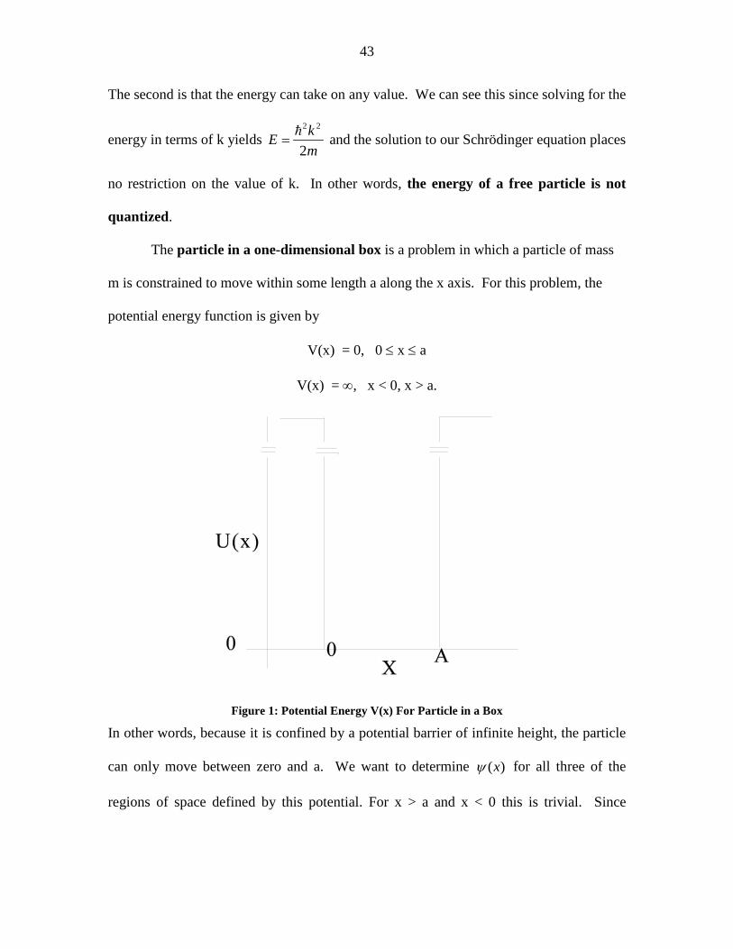
The particle in a one-dimensional box is a problem in which a particle of mass

m is constrained to move within some length a along the x axis. For this problem, the

potential energy function is given by

V(x) = 0, 0 ≤ x ≤ a

V(x) = ∞, x < 0, x > a.

Figure 1: Potential Energy V(x) For Particle in a Box

In other words, because it is confined by a potential barrier of infinite height, the particle

can only move between zero and a. We want to determine ( )xψ for all three of the

regions of space defined by this potential. For x > a and x < 0 this is trivial. Since

44

( )V x = ∞ in these regions it is impossible for the particle to be there, and therefore the

probability amplitude, ( )xψ , must be zero everywhere in these regions.

In the region 0 ≤ x ≤ a, V(x) = 0 and the Schrödinger equation is

2

2

(x)x

= - 2mE = -k∂∂ψ ψ ψ2

2

where k = ( 2mE )21/ 2

, just as it was for the free particle. Once again the general solution

to this equation is

ψ (x)= A kx+ B kxcos sin .

Remember that ( )xψ must be continuous for all values of x. The region where we have

to pay particular attention to this is at the boundary of the region in which the particle

moves. At x = 0, ψ must be equal to zero, since ψ = 0 for x<0. Similarly at x = a, ψ

must also equal zero, since ψ = 0 for all x > a. We call these constraints on the value of

ψ at the boundary of our potential well boundary values.

These boundary values place constraints on our solution. We see the first of

these by setting x = 0 and setting ψ = 0 in compliance with our first boundary value. This

gives us

ψ (0)= 0 = A 0+ B 0 = A.cos sin

Therefore A = 0 and our wavefunction simplifies to

ψ (x)= B kx.sin

We see our second constraint by applying our second boundary condition, setting x = a

and ψ = 0. This gives us

ψ (a)= 0 = B kasin

45

This will only equal zero when ka = π, 2π, 3π,..., nπ,.... Therefore we can write

k = naπ .

and our wavefunction becomes

ψ π(x)= B n xa

sin

If we normalize this as before, we get finally,

ψ π(x)= ( 2a

) n xa

1/ 2 sin

Note that the requirement k = naπ leads to the quantization of the energy of the

particle in a box, since

k = ( 2mE ) = na2

1/ 2

π

Solving this equation for E yields

E = n h8ma

2 2

2 ,

which is quantized because of the presence of the integers in the equation.

Notice that the general solutions to the Schrödinger equation for the free particle

and the particle in a box are identical. The only difference between the two problems is

the presence of the boundaries that constrain the movement of the particle in the particle

in a box. We will find that every time a boundary constrains the motion of a particle,

the energy of that particle will be quantized. In the absence of these constraints the

particle can take on any energy.

What are some of the physical consequences of these results? First, notice that

there is a minimum energy for the particle in a box. The lowest energy is when n= 1 and

46

is equal to 2

1 28hEma

= . This minimum energy is called the zero point energy of the

system. Why can’t n = 0? The reason is that substituting n=0 in our equation for the

wavefunction of the particle in a box yields ψ=0 for all values of x. Since the probability

of finding a particle in a given position is given by *( ) ( )x x dxψ ψ , this means that the

probability of finding a particle in a state with n=0 is identically zero.

There is an interesting corollary to this. If n was 0 the energy would equal zero,

the particle would be motionless and would violate the uncertainty principle, since in

order for the particle to be motionless, it’s position uncertainty would have to be infinite,

and therefore the particle could not be confined to the box. In other words, the

uncertainty principle forbids that any bound system be entirely motionless, i.e., not only

thermodynamics but quantum mechanics forbids any system from reaching absolute zero.

As the quantum number n increases, the energy of the particle increases, with

E 4h8ma2

2

2= , E = 9h8ma3

2

2 . etc.

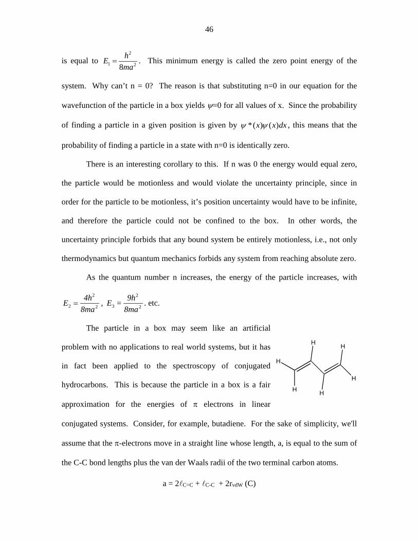
The particle in a box may seem like an artificial

problem with no applications to real world systems, but it has

in fact been applied to the spectroscopy of conjugated

hydrocarbons. This is because the particle in a box is a fair

approximation for the energies of π electrons in linear

conjugated systems. Consider, for example, butadiene. For the sake of simplicity, we'll

assume that the π-electrons move in a straight line whose length, a, is equal to the sum of

the C-C bond lengths plus the van der Waals radii of the two terminal carbon atoms.

a = 2C=C + C-C + 2rvdW (C)

H

H

H

H

H

H

47

= 2 x 135 pm + 154 pm + 2 x 77 pm = 578 pm = 5.78 x 10-10 m.

Thus we will model the electrons as moving in a 5.78 x 10-10 m box. According to the

solution for the particle in a one dimensional box,

nE = n h8ma

2 2

2 ,

where in this case, as we have just shown, a, the length of the box, is equal to 5.78 x 10-10

m. The Pauli exclusion principle, which we will discuss in detail later, tells us that there

can only be two electrons for each quantum number n. Butadiene has four π electrons.

We place two in the lowest state of our particle in a box, n= 1, and the final two in n = 2.

Thus for butadiene, the highest occupied molecular orbital is n = 2, i.e., HOMO = 2. The

lowest unoccupied molecular orbital, LUMO, is n = 3. The electronic absorption should

occur at the energy necessary to promote an electron from the HOMO to the LUMO, i.e.,

from n = 2 to n= 3. The energy of this transition is

∆E(3 2)= hma

- hma

= 9.02x J← −98

48

102

2

2

219

This corresponds to an absorption at 220 nm. Butadiene has an absorption at 217 nm, so

we see that despite its simplicity, the particle in a box is a fairly good model for the

ultraviolet spectra of simple conjugated models.

If we plot the wavefunctions for n = 1, n = 2, etc., we see that they take on the

appearance of standing waves. Notice that n=1 contains 1/2 of a wave, n=2 contains a

full wave, n = 3 contains 3/2 wave, and in general level n will contain n/2 waves, i.e.,

each level contains an integral number of half waves. If we look at the probability

density *ψ ψ for each of these levels, we find that for n = 1 the maximum probability is

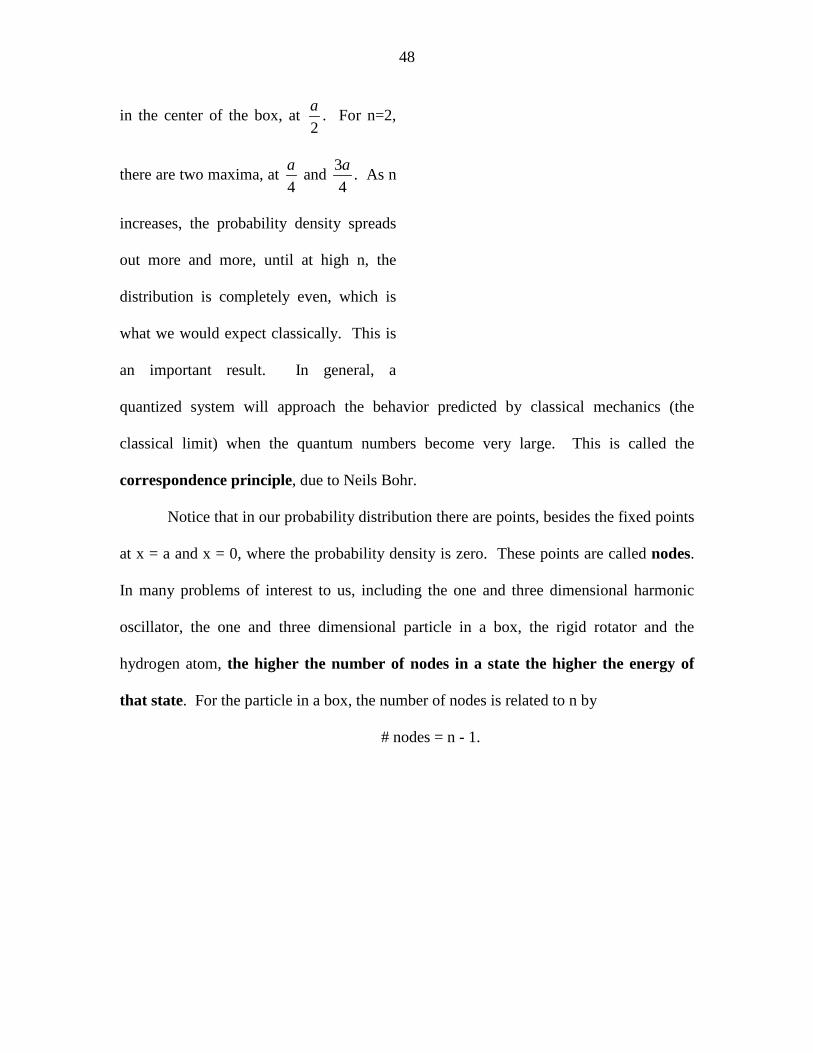
48

in the center of the box, at 2a . For n=2,

there are two maxima, at 4a and 3

4a . As n

increases, the probability density spreads

out more and more, until at high n, the

distribution is completely even, which is

what we would expect classically. This is

an important result. In general, a

quantized system will approach the behavior predicted by classical mechanics (the

classical limit) when the quantum numbers become very large. This is called the

correspondence principle, due to Neils Bohr.

Notice that in our probability distribution there are points, besides the fixed points

at x = a and x = 0, where the probability density is zero. These points are called nodes.

In many problems of interest to us, including the one and three dimensional harmonic

oscillator, the one and three dimensional particle in a box, the rigid rotator and the

hydrogen atom, the higher the number of nodes in a state the higher the energy of

that state. For the particle in a box, the number of nodes is related to n by

# nodes = n - 1.

49

Lecture 8

At this point, we’ve seen our first example of how to solve the Schrödinger

equation. We’ve seen how to use the eigenfunctions we’ve obtained to describe the

probability of finding the system in various positions. We’ve also seen how to extract

information from our eigenfunctions – we determined the energy by operating on our

eigenfunctions with the Hamiltonian (total energy) operator.

However, we still need to learn more about the mechanics of quantum mechanics

– for example, we don’t yet know how to extract information from a wavefunction when

it is not an eigenfunction, i.e., not a solution of an eigenvalue equation. We already have

made a couple of statements about these types of wavefunctions, first that even though

they are not eigenfunctions of our operators, we’ll still always observe only eigenvalues

of the operator but that we can’t predict which one, and second, that we can predict the

probability of observing a given eigenfunction. In order to understand why these

statements are true, we’ll have to learn something about the mathematical properties of

eigenfunctions.

We've already stated that to be consistent with their interpretation as probability

amplitudes, eigenfunctions must be normalized. This condition is usually written as

* 1i jd if i jψ ψ τ∞

−∞= =∫

Another property of a set of eigenfunctions is that the product of two different

eigenfunctions of the same operator integrated over all space is zero, i.e.,

* 0i jd if i jψ ψ τ∞

−∞= ≠∫

50

When two wavefunctions satisfy this equation they are called orthogonal

wavefunctions. So in other words if we generate a set of eigenfunctions by solving the

Schrödinger equation, any two of these functions will be orthogonal.

Our two statements on orthogonality and normalization are usually represented by

a single equation,

*i j ijdψ ψ τ δ

∞

−∞=∫

where δij is called the Kronecker delta function which is defined by

δij = 0, i ≠ j

δij = 1, i = j.

Sets of functions that are both orthogonal and normalized are called orthonormal

functions.

It turns out that all discrete solutions to the Schrödinger equation are complete

orthonormal sets of functions. Complete orthonormal sets of functions are important

because any arbitrary function ψ(x) can be expressed as a linear combination of

members of a complete orthonormal set of functions. Thus any arbitrary

wavefunction ψ(x) can be expressed as a linear combination of eigenfunctions, ψi(x). In

other words,

ψ ψ ψ ψ( ) ( ) ( ) ( ) ...x c x c x c x= + + +1 1 2 2 3 3

where ψ(x) is any arbitrary wavefunction, the ci’s are constants, and the ψi(x) are

eigenfunctions of some operator. This rule, that any arbitrary wavefunction can be

expressed as a linear combination of eigenfunctions, is sometimes referred to as the

superposition principle.

51

This explains why we observe only eigenvalues even when our wavefunction ψ(x)

is not itself an eigenfunction. We are observing the eigenvalue of one of the

eigenfunctions that make up our wavefunction. The probability of observing one of

these eigenvalues is equal to the square of its coefficient, ci2. This implies that the sum of

the squares of the coefficients must be one, i.e.,

cii

2 1∑ = .

Sometimes two eigenfunctions will have the same energy. In this case we say

that the eigenfunctions are degenerate. One property of degenerate eigenfunctions is

that all linear combinations of degenerate eigenfunctions will also be eigenfunctions.

This is not true for nondegenerate eigenfunctions.

Note that while the solutions we have obtained for the particle in a box are

eigenfunctions of the Hamiltonian operator they are not eigenfunctions of the position

operator X . If this was so, X (x)= x (x)ψ ψ would equal a constant times ψ(x), which is

not the case. According to our postulates, if we have a state ( )xψ which is an

eigenfunction of the Hamiltonian but NOT and eigenfunction of the operator X , we will

obtain an eigenvalue of some eigenfunction of the operator X when we measure x, but

we won't be able to predict which one. Repeated measurement of x will yield the

probability densities we have calculated.

Even though we cannot predict the value of a given measurement when a

wavefunction is not an eigenfunction of the operator in question, we can always

predict the average value of the measurement. For this we need another postulate.

52

To introduce this postulate, we'll begin with a review of averages. Most of us are

introduced to averages of what are called discrete distributions. The numbers you

obtain by rolling a die are a discrete distribution, with the integers 1-6 the only possible

results, and no intervening numbers possible. Discrete distributions are intrinsically

discontinuous. In this case, the procedure for taking an average is simple. If you roll the

die 5 times, you add the five numbers, divide by 5 and you have the average. For

example if five rolls got you 1,3,2,4,3, your average is (1+3+2+4+3)/5 = 2.6. In general

the average of N measurements of some observable F is given by

FF

N

n

N

=∑

1 ,

where the brackets indicate an average value. An alternative way of calculating the

average for a discrete distribution is with the equation

F p Fff

N

f==∑

1

where pf is the probability that the result Ff is observed. In our example above, the

probability of observing 1,2, and 4 was 1 in 5 or .2, while the probability of observing 3

was 2 in 5 or .4, and the probability of observing 5 and 6 was zero. Our average is 1 x .2

+ 2 x .2 + 3 x .4 + 4 x .2 + 5 x 0 + 6 x 0 = 2.6. The set of probabilities, {pf }, is called a

discrete probability distribution.

If our measurements can vary continuously, as would be the case for the

measurement of a series of lengths, the average is calculated using a continuous

53

probability distribution in place of the discrete probability distribution. If our

continuous probability distribution is given by f(x)dx, then the average of some variable x

is given by

-x xf(x)dx

∞

∞= ∫

This fits nicely into our quantum mechanical formulation, since ψ*(x)ψ(x)dx is a

continuous probability distribution. However, there's a bit of a twist in quantum

mechanics. A postulate of quantum mechanics says that the average of a quantum

mechanical observable A, is given by

* ˆ( ) ( )a x A x dxψ ψ∞

−∞= ∫

Note that this equation does two things. The operator operating on ψ extracts the value

or values of A that can be observed, and then the product with *ψ gives us our average.

Note that if ψ(x) is an eigenfunction of A , then <a> is simply the eigenvalue of A , an.

LET'S PROVE THIS CLAIM TOGETHER. LET'S LOOK AT A SIMPLE LINEAR COMBINATION OF

EIGENFUNCTIONS, ψ = C1ψ1(X) + C2ψ2(X) AND SEE WHAT ITS AVERAGE IS.

Let’s do a quick example and calculate the average position for the particle in a

box. We'll make this a bit fancy and rather than calculate the average for a given state,

we'll calculate a formula so we can see what the average is for any value of n. Before I

actually calculate the average, let’s look at the probability density for a few states.

[DRAW] CAN ANYONE PREDICT WHAT THE AVERAGE POSITION WILL BE? [a/2] The average

is in the middle of our range of possible x values because our potential function is

symmetric about the range of x. In general we will find that any time we have a

54

symmetric potential function our probability density will be symmetric as well. The

wavefunction for the particle in a box is

n1/ 2= ( 2

a) n x

aψ πsin

Therefore the average of x over the range 0 to a is given by

1/ 2 1/ 2 2

0 0

2sin sin sina a2 n x 2 n x n xx ( x( dx x dx) )

a a a a a aπ π π

= =∫ ∫

This integral while difficult can be found in any standard table of integrals and yields

22 a ax ( )a 4 2

= =

Note that this calculation yields the same result as our qualitative prediction of the

probability density, that the average position is the same for all states of the particle in a

box.

In addition to being able to calculate the average of an observable quantity, it is

useful to know how widely a measurement is spread around the average. A useful

measurement of this is the variance, σx2. The variance is the square of a function that you

are all familiar with, the standard deviation, σx. Because of the manner in which we

calculate quantum mechanical averages, in quantum mechanics the variance is most

easily calculated by using the formula

σ x x x2 2 2= < > − < >

Before we go ahead and calculate the spread, let’s go back and look at our probability

density for the particle in a box. WHAT IS THE TENDENCY IN THE SPREAD OF THE

DISTRIBUTION AS WE GO UP IN ENERGY? In order to calculate the variance we need to be

55

able to calculate <x2>. WHAT IS THE FORMULA FOR THE AVERAGE OF X2? So for the

particle in a box,

1/ 2 1/ 22 2 2 2

0 0

2sin sin sina a2 n x 2 n x n xx ( x ( dx x dx) )

a a a a a aπ π π

= =∫ ∫

Of course, we look this up in our handy table of integrals to find that

2 22 2 4( ) ( 2)

2 3a nx

nπ

π= −

Since we now know <x> and <x2>, we can calculate the variance,

2 22 22 2

xa nx x ( ( - 2))

2 n 3πσ

π= − =

If you plot the variance as a function of n you will find that this formula matches our

intuition and that as n increases the probability distribution gets wider. AS A HOMEWORK

ASSIGNMENT, CALCULATE THIS VARIANCE FOR N = 1 TO 10, FOR A BOX WITH A = 1.00 NM.

So we now have two tools to help us understand the nature of a probability distribution,

the average or expectation value and the variance. One way that the variance is used is as

a measure of the uncertainty of an observable. The larger the variance, the larger the

uncertainty.

56

Lecture 9

Many of the problems that are of the greatest interest to chemists are

multidimensional. For example, the rigid rotor, the simplest model of a rotating

molecule, is two dimensional, while the hydrogen atom is three dimensional, and the

vibration of polyatomic molecules turns out to be 3N-6 dimensional, where N is the

number of atoms in the molecule. While each of these problems has its own unique

features, all of them have certain common features. We can see what these are by

studying the simplest three-dimensional problem, the particle in a three-dimensional

box.

In this problem the particle is contained in a box with sides of length a, b, and c.

Outside of the box the potential is ∞. We write this as the set of conditions

V = 0 , 0 ≤ x ≤ a; 0 ≤ y ≤ b; 0 ≤ z ≤ c

V = ∞, elsewhere.

The Schrödinger equation for a single particle moving in three dimensions is

( , , ) ( , , )H x y z E x y zψ ψ=

where

H2m

V(x, y,z)= − ∇ +

22 ,

and where ∇2 is called the Laplacian, which is the dot product of two gradients, where the

gradient ∇ is defined as

i j kx y z∂ ∂ ∂

∇ = + +∂ ∂ ∂

,

57

and is a vector quantity where i

, j

, and k

are unit vectors along the x, y and z axes

respectively. The dot product of the gradient with itself, the Laplacian, is a scalar

quantity and is equal to

22 2 2

2 2 2

+ +x y z∂ ∂ ∂∇ = ∇⋅∇ =∂ ∂ ∂

.

So we see that two differences in our three dimensional case are that the wavefunctions

will be functions of x, y, and z, and the partials are taken not just with respect to x,

but with respect to y and z as well. For a wavefunction in three dimensions, the

probability density is * (x, y,z) (x, y,z)ψ ψ , the probability that a particle will be found in

an infinitesimal volume near x,y,z is given by

prob{x,x+ dx; y, y+ dy,z,z+ dz} = (x, y,z) (x, y,z)dxdydz*ψ ψ ,

while the probability that we will find the particle in the finite volume bounded by x1, x2,

y1, y2, z1 and z2, is given by the triple integral,

{ } 2 2 2

1 1 1

*1 2 1 2 1 2, ; , ; , ( , , ) ( , , )

x y z

x y zprob x x y y z z x y z x y z dxdydzψ ψ= ∫ ∫ ∫

Since this integral, as was the case for the one-dimensional problem, is also a probability,

we have the same requirements as before for normalizability, single valuedness and

continuity.

A multiple integral is sort of a partial derivative in reverse. What you do is

choose one variable to integrate at a time and hold the others constant. Then you choose

the next and so on. For example, consider the integral of the simple function xy + yz +

zx. The full triple integral is

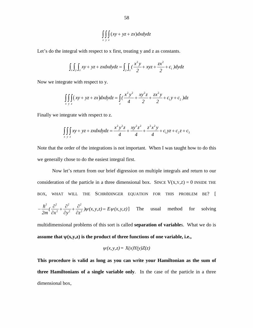
58

( )x y z

xy yz zx dxdydz+ +∫ ∫ ∫

Let’s do the integral with respect to x first, treating y and z as constants.

2 2

1x y z y z

x y zxxy yz zxdxdydz ( xyz c )dydz2 2

+ + = + + +∫ ∫ ∫ ∫ ∫

Now we integrate with respect to y.

( )2 2 2 2

1 2x y z z

x y xy z zx yxy yz zx dxdydz ( c y c )dz4 2 2

+ + = + + + +∫ ∫ ∫ ∫

Finally we integrate with respect to z.

2 2 2 2 2 2

1 2 3x y z

x y z xy z z x yxy yz zxdxdydz c yz c z c4 4 4

+ + = + + + + +∫ ∫ ∫

Note that the order of the integrations is not important. When I was taught how to do this

we generally chose to do the easiest integral first.

Now let’s return from our brief digression on multiple integrals and return to our

consideration of the particle in a three dimensional box. SINCE V(X,Y,Z) = 0 INSIDE THE

BOX, WHAT WILL THE SCHRöDINGER EQUATION FOR THIS PROBLEM BE? [

− ∂∂

+ ∂∂

+ ∂∂

=2 2 2 2

2m(

x y z) (x, y,z) E (x, y,z)

2 2 2 ψ ψ ] The usual method for solving

multidimensional problems of this sort is called separation of variables. What we do is

assume that ψ(x,y,z) is the product of three functions of one variable, i.e.,

ψ (x, y,z)= X(x)Y(y)Z(z)

This procedure is valid as long as you can write your Hamiltonian as the sum of

three Hamiltonians of a single variable only. In the case of the particle in a three

dimensional box,

59

( ) H = -2m

(x

+y

+z

)= -2m x

-2m y

-2m z

= H (x)+ H y + H (z)2 2 2 2 2 2 2 2 2 2 ∂

∂∂∂

∂∂

∂∂

∂∂

∂∂2 2 2 2 2 2 1 2 3

Since we've broken down our Hamiltonian into three Hamiltonians of one variable each,

separation of variables is valid for this problem. The effect of separation of variables is

to break our problem down into three one-dimensional problems,

H X(x)= E X(x)x x

H Y(y)= E Y(y)y y

H Z(z)= E Z(z)z z

where the total energy E = Ex + Ey + Ez. Since each of these one dimensional problems is

exactly the same as the one dimensional particle in a box, we can immediately write

down solutions for X(x), Y(y) and Z(z).

X(x)= ( 2a

) n xa

,E = n h8max

x1 22 2

2/ sin π

Y(y)= ( 2b

) n yb

,E = n h8mby

y1 22 2

2/ sin π

Z(z)= ( 2c

) n zc

,E = n h8mcz

z1 22 2

2/ sin π

This means that

ψ π π π(x, y,z)= X(x)Y(y)Z(z)= ( 8abc

) n xa

n yb

n zc

1/ 2 sin sin sin

and

x y zn ,n ,n x y zx y zE E E E h

8m( n

anb

nc

)= + + = + +2 2

2

2

2

2

2

60

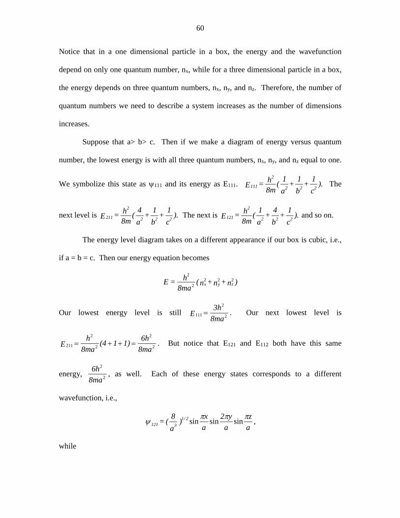
Notice that in a one dimensional particle in a box, the energy and the wavefunction

depend on only one quantum number, nx, while for a three dimensional particle in a box,

the energy depends on three quantum numbers, nx, ny, and nz. Therefore, the number of

quantum numbers we need to describe a system increases as the number of dimensions

increases.

Suppose that a> b> c. Then if we make a diagram of energy versus quantum

number, the lowest energy is with all three quantum numbers, nx, ny, and nz equal to one.

We symbolize this state as ψ111 and its energy as E111. 111

2

2 2 2E = h8m

( 1a

+ 1b

+ 1c

). The

next level is 211

2

2 2 2E = h8m

( 4a

+ 1b

+ 1c

). The next is 121

2

2 2 2E = h8m

( 1a

+ 4b

+ 1c

). and so on.

The energy level diagram takes on a different appearance if our box is cubic, i.e.,

if a = b = c. Then our energy equation becomes

E = h8ma

(n + n + n )x y z

2

22 2 2

Our lowest energy level is still 111

2

2E3h

8ma= . Our next lowest level is

211

2

2

2

2Eh

8ma(4 1 1) 6h

8ma= + + = . But notice that E121 and E112 both have this same

energy, 6h8ma

2

2 , as well. Each of these energy states corresponds to a different

wavefunction, i.e.,

121 31/ 2= ( 8

a) x

a2 ya

za

,ψ π π πsin sin sin

while

61

211 31/ 2= ( 8

a) 2 x

ay

az

a,ψ π π πsin sin sin

yet their energies are the same. When two or more different wavefunctions have the

same energy, we say that they are degenerate. Degenerate states are always due to

some symmetry in the system. For example, in this case, when a=b=c, the system has

degenerate states. If a = b ≠ c, there are also degenerate states because as in our first case

there is a level of symmetry. You can see this because for this case

E = h8m

( n + na

+ nc

)n n n

2x2

y2

2z2

2x y z,

which means that

211 121

2

2 2E = E = h8m

( 5a

+ 1c

) while 112

2

2 2E = h8m

( 2a

+ 4c

).

However, for the case where a ≠ b ≠ c, and there is no other symmetry, there are no

degenerate states. Degenerate states are at the core of several phenomena, the most

familiar of which is NMR.

To summarize: If you have a Hamiltonian, H , which can be written as the

sum of component Hamiltonians of one variable, H = H H H ,x y z+ + then the

solution, ψ(x,y,z), will be the product of three one dimensional wavefunctions,

ψ (x, y,z)= X(x)Y(y)Z(z) , and its energy will be the sum of the eigenvalues of the one

dimensional eigenvalue equations, E = Ex + Ey + Ez.