Lectures 12–21

Random Variables

Definition: A random variable (rv or RV) is a real valued function defined on the sample space.The term “random variable” is a misnomer, in view of the normal usage of function and variable.Random variables are denoted by capital letters from the end of the alphabet, e.g. X, Y , Z,but other letters are used as well, e.g., B, M , etc.Hence: X : S 7−→ R and X(e) for e ∈ S is a particular value of X. Since the e are randomoutcomes of the experiment, it will make the function values X(e) random as a consequence.Hence the terminology “random variable”, although “random function value” might have beenless confusing. Random variables are simply a bridge from the sample space to the realm ofnumbers, where we can perform arithmetic.A random variable is different from a random function, where the evaluation for each e is afunction trajectory, e.g., against time as in a stock market index for a given day. Such randomfunctions are also known as stochastic processes. We will only have limited exposure to them.Example 1 (Roll of Two Dice): The sum X of the two numbers facing up is an rv.Example 2 (Toss of Three Coins): The number X of heads in the toss of three coins is arandom variable. Compute P (X = i) = P ({X = i}) for i = 0, 1, 2, 3. The event {X = i} standsshort for {e ∈ S : X(e) = i}.Example 3 (Urn Problem): Three balls are randomly selected (without replacement) from anurn containig 20 balls labeled 1, 2, . . . , 20. We bet that we will get at least one label ≥ 17.What is the probability of winning the bet. This problem could be solved without involving thenotion of a random variable. For the sake of working with the concept of a random variable let Xbe the maximum number of the three balls drawn. Hence we are interested in P (X ≥ 17), whichis computed as follows:

P (X ≥ 17) = P (X = 17) + P (X = 18) + P (X = 19) + P (X = 20) = 1− P (X ≤ 16)

with P (X = i) =

(i−12

)(203

) for i = 3, 4, . . . , 20 ,

=⇒ P (X ≥ 17) =

(162

)(203

) +

(172

)(203

) +

(182

)(203

) +

(192

)(203

) =2

19+

34

285+

51

380+

3

20= .50877 = 1−

(163

)(203

)Example 4 (Coin Toss with Stopping Rule): A coin (with probability p of heads) is tosseduntil either a head is obtained or until n tosses are made. Let X be the number of tosses made.Find P (X = i) for i = 1, . . . , n.Solution: P (X = i) = (1− p)i−1p for i = 1, . . . , n− 1 and P (X = n) = (1− p)n−1.Check that probabilities add to 1.

Example 5 (Coupon Collector Problem): There are N types of coupons. Each time a couponis obtained, it is, independently of previous selections, equally likely to be one of the N types. Weare interested in the random variable T = the number of coupons that needs to be collected to geta full set of N coupons. Rather than get P (T = n) immediately, we obtain P (T > n).

1

Let Aj be the event that coupon j is not among the first n collected coupons. By the inclusion-exclusion formula we have

P (T > n) = P

(N⋃i=1

Ai

)=

N∑i=1

P (Ai)−∑i1<i2

P (Ai1Ai2) + . . .+ (−1)N+1P (A1A2 . . . AN)

with P (A1A2 . . . AN) = 0, of course, and for i1 < i2 < . . . we have

P (Ai) =(N − 1

N

)n, P (Ai1Ai2) =

(N − 2

N

)n, . . . , P (Ai1Ai2 . . . Aik) =

(N − kN

)nand thus

P (T > n) = N(N − 1

N

)n−(N

2

)(N − 2

N

)n+

(N

3

)(N − 3

N

)n− . . .+ (−1)N

(N

N − 1

)(1

N

)n

=N−1∑i=1

(−1)i+1

(N

i

)(N − iN

)nand P (T > n− 1) = P (T = n) + P (T > n), hence P (T = n) = P (T > n− 1)− P (T > n).

Distribution Functions

Example 6 (First Heads): Toss fair coin until first head lands up. Let X be the number oftosses required. Then P (X ≤ k) = 1− P (X ≥ k + 1) = 1− P (k tails in first k tosses) = 1− 0.5k.

Definition: The cumulative distribution function (cdf or CDF) or more simply the distibutionfunction F of the random variable X is defined for all real numbers b as L12

endsF (b) = P (X ≤ b) = P ({e : X(e) ≤ b}) .

Example 7 (Using a CDF): Suppose the cdf of the random variable X is given by

F (x) =

0 x < 0x2

0 ≤ x < 123

1 ≤ x < 21112

2 ≤ x < 3

1 3 ≤ x

x

F(x

)

−1 0 1 2 3 4

0.0

0.2

0.4

0.6

0.8

1.0

●

●

●

Compute P (X < 3), P (X = 1), P (X > .5) and P (2 < X ≤ 4).1112

, 23− 1

2= 1

6, 1− .5

2= .75, 1− 11

12= 1

12.

2

Discrete Random Variables

Definition: A random variable X which can take on at most a countable number of values iscalled a discrete random variable. For such a discrete random variable we define its probabilitymass function (pmf) p(a) of X by

p(a) = P (X = a) = P ({e : X(e) = a}) for all a ∈ R .

p(a) is positive for at most a countable number of values of a. If X assumes only one of thefollowing values x1, x2, x3, . . . then

p(xi) ≥ 0 for i = 1, 2, 3, . . . and p(x) = 0 for all other values of x

Graphical representation of p(x) (one die, sum of two dice):Example 8 (Poisson): Suppose the discrete random variable X has pmf p(i) = cλi/i! fori = 0, 1, 2, . . . where λ is some positive value and c = exp(−λ) makes the probabilities add toone. Find P (X = 0) and P (X > 2). P (X = 0) = c = exp(−λ),P (X > 2) = 1− P (X = 0)− P (X = 1)− P (X = 2) = 1− exp(−λ)(1 + λ+ λ2/2).The cdf F of a discrete random variable X can be expressed as

F (a) =∑x: x≤a

p(x) .

The c.d.f. of a discrete random variable X is a step function with a possible step at each of itspossible values x1, x2, . . . and being flat in between.Example 9 (Discrete CFD): p(1) = .25, p(2) = .5, p(3) = .125 and p(4) = .125, construct thec.d.f. and graph it. Interpret the step size.

Expected Value or Mean of X

A very important concept in probability theory is that of the expected value or mean of arandom variable X. For a discrete RV it is defined as

E[X] = E(X) = µ = µX =∑

x:p(x)>0

x · p(x) =∑x

x · p(x)

the probability weighted average of all possible values of X.If X takes on the two values 0 and 1 with probabilities p(0) = .5 and p(1) = .5 thenE[X] = 0 · .5 + 1 · .5 = .5, which is half way between 0 and 1.When p(1) = 2/3 and p(0) = 1/3, then E[X] = 2/3, twice as close to 1 than to 0. That’s becausethe probability of 1 is twice that of 0. The double weight 2/3 at 1 balances the weight of 1/3 at 0,when the fulcrum of balance is set at 2/3 = E[X].weight1 ·moment arm1 = weight2 ·moment arm2 or 2/3 · 1/3 = 1/3 · 2/3, where the moment armis measured as the distance of the weight from the fulcrum, here at 2/3 = E[X].moment arm1 = |2/3− 1| = 1/3 and moment arm2 = |2/3− 0| = 2/3This is a general property of E[X], not just limited to RVs with two values.If a is the location of the fulcrum, then we get balance when∑x<a

(a− x)p(x) =∑x>a

(x− a)p(x) or 0 = −∑x<a

(a− x)p(x) +∑x>a

(x− a)p(x) =∑x

(x− a)p(x)

3

or 0 =∑x

xp(x)− a∑x

p(x) or 0 = E[X]− a or a = E[X]

L13endsThe term expectation can again be linked to our long run frequency motivation for probabilities.

If we play the same game repeatedly, say a large number N times, with payoffs being one of theamounts x1, x2, x3, . . ., then we would roughly see these amounts with approximate relativefrequencies p(x1), p(x2), p(x3), . . ., i.e., with approximate frequencies Np(x1), Np(x2), Np(x3), . . .,thus realizing in N such games the following total payoff:

Np(x1) · x1 +Np(x2) · x2 +Np(x3) · x3 + . . .

i.e., on a per game basis

Np(x1) · x1 +Np(x2) · x2 +Np(x3) · x3 + . . .

N= p(x1) · x1 + p(x2) · x2 + p(x3) · x3 + . . . = E[X]

On average we expect to win E[X] (or lose E[X], if E[X] < 0).

Example 10 (Rolling a Fair Die): If X is the number showing face up on a fair die, we get

E[X] =1

6· 1 +

1

6· 2 +

1

6· 3 +

1

6· 4 +

1

6· 5 +

1

6· 6 =

3 · 76

=7

2

Indicator Variable: For any event E we can define the indicator RV

I = IE(e) = 1 if e ∈ E and IE(e) = 0 if e /∈ E ⇒ E[I] = P (E) · 1 + P (Ec) · 0 = P (E)

Example 11 (Quiz Show): You are asked two different types of questions, but the second oneonly when you answer the first correctly. When you answer a question of type i correctly you geta prize of Vi dollars. In which order should you attempt to answer the question types, when youknow your chances of answering questions of type i are Pi, i = 1, 2, respectively? Or does theorder even matter? Assume that the events of answering questions are independent?If you choose to answer a question of type i = 1 first, your winnings are

0 with probability 1− P1

V1 with probability P1(1− P2)V1 + V2 with probability P1P2

with expected winnings W1: E[W1] = V1P1(1− P2) + (V1 + V2)P1P2.When answering the type 2 question first, you get the same expression with indices exchanged,i.e., E[W2] = V2P2(1− P1) + (V1 + V2)P1P2. Thus

E[W1] > E[W2] ⇐⇒ V1P1(1− P2) > V2P2(1− P1) ⇐⇒V1P1

1− P1

>V2P2

1− P2

the choice should be ordered by odds-weighted payoffs. Example: P1 = .8, V1 = 900, P2 = .4,V2 = 6000, then 900·.8

.2= 3600 < 6000·.4

.6= 4000. E[W1] = 2640 < E[W2] = 2688.

4

Expectation of g(X): For an RV X and a function g : R→ R, we can view Y = g(X) again asa random variable. Find its expectation.Two ways: Find the pX(x)-weighted average of all g(X) values, or given the pmf pX(x) of X, findthe pmf pY (y) of Y = g(X), then its expectation as the pY (y) weighted average of all Y values.Example: Let X have values −2, 2, 4 with p(X(−2) = .25, pX(2) = .25, pX(4) = .5, respectively.

=⇒

x pX(x) x2 x2pX(x)-2 .25 4 12 .25 4 14 .5 16 8

10

=⇒

y = x2 pY (y) ypY (y)4 .5 216 .5 8

10

∑x

x2pX(x) = (−2)2 · .25 + 22 · .25 + 42 · .5 = 4 ·pY (4)︷ ︸︸ ︷

(.25 + .25) +16 · .5 =∑y

ypY (y) = 10

What we see in this special case holds in general for discrete RVs X and functions Y = g(X)

E[Y ] =∑y

ypY (y) =∑x

g(x)pX(x) = E[g(X)]

The formal proof idea is already contained in the above example, so we skip it, but see book fornotational formal proof or the graphic above.

5

Example 12 (Business Planning): A seasonal product (say skis), when sold in timely fashion,yields a net profit of b dollars for each unit sold, and a net loss of ` dollars, when it needs to besold at season’s end at a fire sale. Assume that the customer demand for the number X of unitsis an RV with pmf pX(x) = p(x) and assume s units are stocked. When X > s, the excess orderscannot be filled. Then the realized profit Q(s) is an RV, namely

Q(s) =

{bX − (s−X)` if X ≤ ssb if X > s

with expected profit

E[Q(s)] =s∑i=0

(bi− (s− i)`)p(i) + sb∞∑

i=s+1

p(i) = (b+ `)s∑i=0

ip(i)− s`s∑i=0

p(i) + sb

[1−

s∑i=0

p(i)

]

= (b+ `)s∑i=0

ip(i)− s(b+ `)s∑i=0

p(i) + sb = sb+ (b+ `)s∑i=0

(i− s)p(i)

Find the value s that maximizes this expected value.We examine what happens to E[Q(s)] as we increase s to s+ 1.

E[Q(s+ 1)] = (s+ 1)b+ (b+ `)s+1∑i=0

(i− s− 1)p(i) = (s+ 1)b+ (b+ `)s∑i=0

(i− s− 1)p(i)

=⇒ E[Q(s+ 1)]− E[Q(s)] = b− (b+ `)s∑i=0

p(i) > 0 ⇐⇒s∑i=0

p(i) <b

b+ `

Since∑si=0 p(i) increases with s and since b/(b+ `) is constant, there is a largest s, say s∗, for

which this inequality holds, and thus the maximum expected profit is E[Q(s∗ + 1)], achievedwhen stocking s∗ + 1 items. We need to know p(i), i = 0, 1, . . ., e.g., from past experience.

Examples of E[g(X)]: 1) Let g(x) = ax+ b, with constants a, b, then

E[aX + b] =∑x

(ax+ b)p(x) = a∑x

xp(x) + b∑x

p(x) = aE[X] + b

2) let g(x) = xn, thenE[Xn] =

∑x

xnp(x)

is called the nth moment of X,and E[X] is also known as the first moment. L14ends

The Variance of X

While E[X] is a measure of the center of a distribution given by a pmf p(x), we also like to havesome measure of the spread or variation of a distribution. While E[X] = 0 for X ≡ 0 withprobability 1, or X = ±1 with probability 1/2 each or X = ±100 with probability 1/2 each, wewould view the variabilities of these three situations quite differently. One plausible measurewould be the expected absolute difference of X from its mean, i.e., E[|X − µ|], where µ = E[X].For the above three situations we would get E[|X − µ|] = 0, 1, 100, respectively. While this waseasy enough, it turns out the the absolute value function |X − µ| is not very conducive to

6

manipulations. We introduce a different measure that can be exploited much more convenientlyas we will see later on.Definition: The variance of a random variable X with mean µ = E[X] is defined as

var(X) = E[(X − µ)2]

An alternate formula, and example of the manipulative capability of the variance definition, is

var(X) = E[X2 − 2µX + µ2] =∑x

(x2 − 2µx+ µ2)p(x) =∑x

x2p(x)−∑x

2µxp(x) +∑x

µ2p(x)

= E[X2]− 2µE[X] + µ2 = E[X2]− µ2 = E[X2]− (E[X])2

Example 13 (Variance of a Fair Die): If X denotes the face up of a randomly rolled fair diethen

E[X2] =1

612 +

1

622 +

1

632 +

1

642 +

1

652 +

1

662 =

91

6and var(X) =

91

6−(

7

2

)2

=35

12

Variance of aX + b: For constants a and b we have var(aX + b) = a2var(X), since

var(aX + b) = E[{(aX + b− (aµ+ b)}2] = E[a2(X − µ)2] = a2E[(X − µ)2] = a2var(X)

In analogy to the center of gravity interpretation of E[X] we can view var(X) as the moment ofinertia of the pmf p(x), when viewing p(x) as weight in mechanics.

While squaring the deviation of X around µ in the definition of var(X), it creates a distortionand changes any units of measurements to square units. To bring matters back to its originalunits we take the square root of the variance, i.e., the standard deviation SD(X), as theappropriate measure of spread

SD(X) = σ = σX =√

var(X)

We now discuss several special discrete distributions.

Bernoulli and Binomial Random Variables

Aside from the constant random variable which takes on only one value, the next level ofsimplicity is a random variable with only two values, most often 0 and 1, (canonical choice).Definition (Bernoulli Random Variable): A random variable X which can take on only thetwo values 0 and 1 is called a Bernoulli random variable. We indicate its distribution byX ∼ B(p). In liberal notational usage we also write P (X ≤ x) = P (B(p) ≤ x).Such random variables are often employed when we focus on an event E in a particular randomexperiment. Let p = P (E). If E occurs we say the experiment results in a success and otherwisewe call it a failure. The Bernoulli rv X is then defined as follows: X(e) = 1 if e ∈ E andX(e) = 0 if e 6∈ E. Hence X counts the number successes in one performance of the experiment.Often the following alternate notation is used: IE(e) = 1 if e ∈ E and IE(e) = 0 otherwise. IE isthen also called the indicator function of E.

7

The probability mass function of X or IE is

p(0) = P (X = 0) = P ({e : X(e) = 0}) = P (Ec) = 1− pp(1) = P (X = 1) = P ({e : X(e) = 1}) = P (E) = p

where p is usually called the success probability. The mean and variance of X ∼ B(p) is

E[X] = (1− p) · 0 + p · p = p and var(X) = E[X2]− (E[X])2 = E[X]− p2 = p− p2 = p(1− p)

where we exploited X ≡ X2.If we perform n independent repetitions of this basic experiment, i.e. n independent trials, thenwe can talk of another random variable Y , namely the number of successes in these n trials. Y iscalled a binomial random variable and we indicate its distribution by Y ∼ Bin(n, p), againliberally writing P (Y ≤ y) = P (Bin(n, p) ≤ y).For parameters n and p, the probability mass function of Y is (as derived previously)

p(i) = P (Y = i) =

(n

i

)pi(1− p)n−i for i = 0, 1, 2, . . . , n .1

Example 14 (Coin Flips): Flip 5 fair coins and denote by X the number of heads in these 5flips. Get the probability mass function of X.Example 15 (Quality Assurance): A company produces parts. The probability that anygiven part will be defective is .01. The parts are shipped in batches of 10 and the promise ismade that any batch with two or more defectives will be replaced by two new batches of 10 each.What proportion of the batches will need to be replaced?Solution: 1− P (X = 0)− P (X = 1) = 1− (1− p)10 − 10p(1− p)9 = .0043 where p = .012. Henceabout .4% of the batches will be affected.

Example 16: (Chuck-a-luck): A player bets on a particular number i = 1, 2, 3, 4, 5, 6 of a fairdie. The die is rolled 3 times and if the chosen bet number appears k = 1, 2, 3 times the playerwins k units, otherwise loses 1 unit. If X denotes the payoff, what is the expected value E[X] ofthe game?

P (X = −1) =

(3

0

)(1

6

)0 (5

6

)3

=125

216, P (X = 1) =

(3

1

)(1

6

)1 (5

6

)2

=75

216,

P (X = 2) =

(3

2

)(1

6

)2 (5

6

)1

=15

216, P (X = 3) =

(3

3

)(1

6

)3 (5

6

)0

=1

216

=⇒ E[X] = −1 · 125

216+ 1 · 75

216+ 2 · 15

216+ 3 · 1

216=−17

216

with an expected loss of 0.0787 units per game in the long run. L15endsExample 17 (Genetics): A particular trait (eye color or left-handedness) on a person is

governed by a particular gene pair, which can either be {d, d}, {d, r} or {r, r}. The dominant

1With appropriate values for i, n and p you get p(i) via the command dbinom(i,n,p) in R, while pbinom(i,n,p)returns P (Y ≤ i). In EXCEL get these via =BINOMDIST(i,n,p,FALSE) and =BINOMDIST(i,n,p,TRUE), respectively.You may also use the spreadsheet available within the free OpenOffice http://www.openoffice.org/.

21-pbinom(1,10,.01) in R and in EXCEL via = 1-BINOMDIST(1,10,.01,TRUE).

8

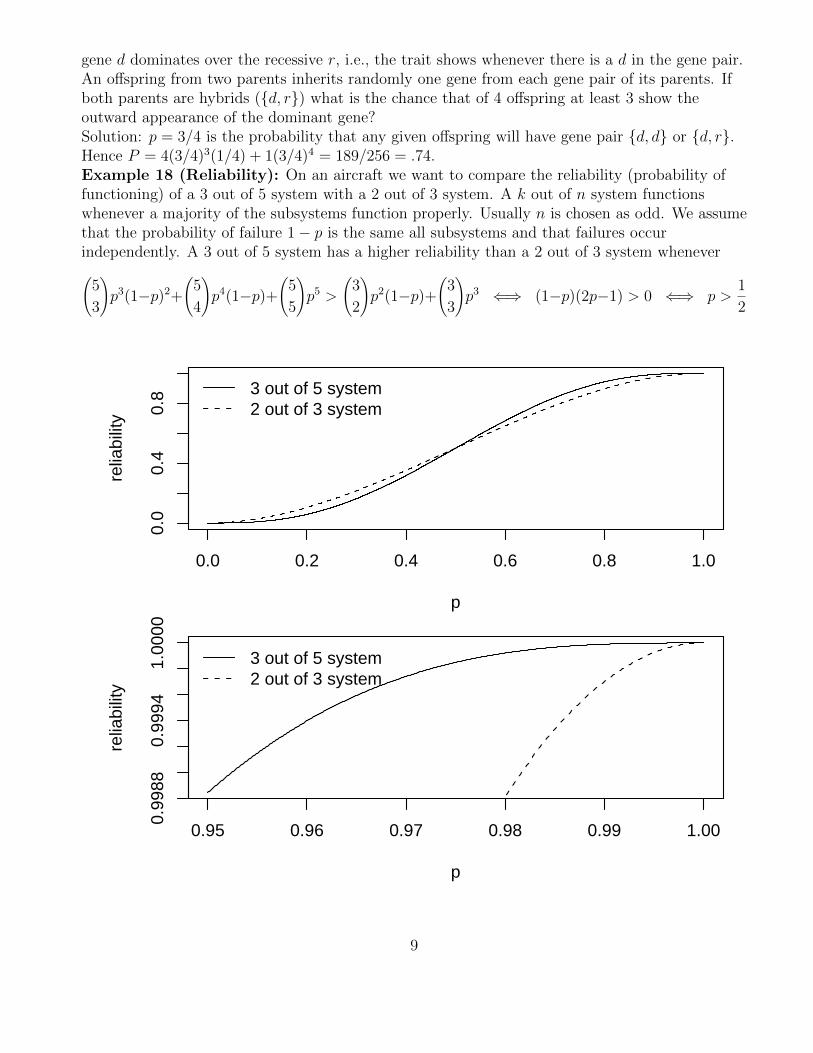
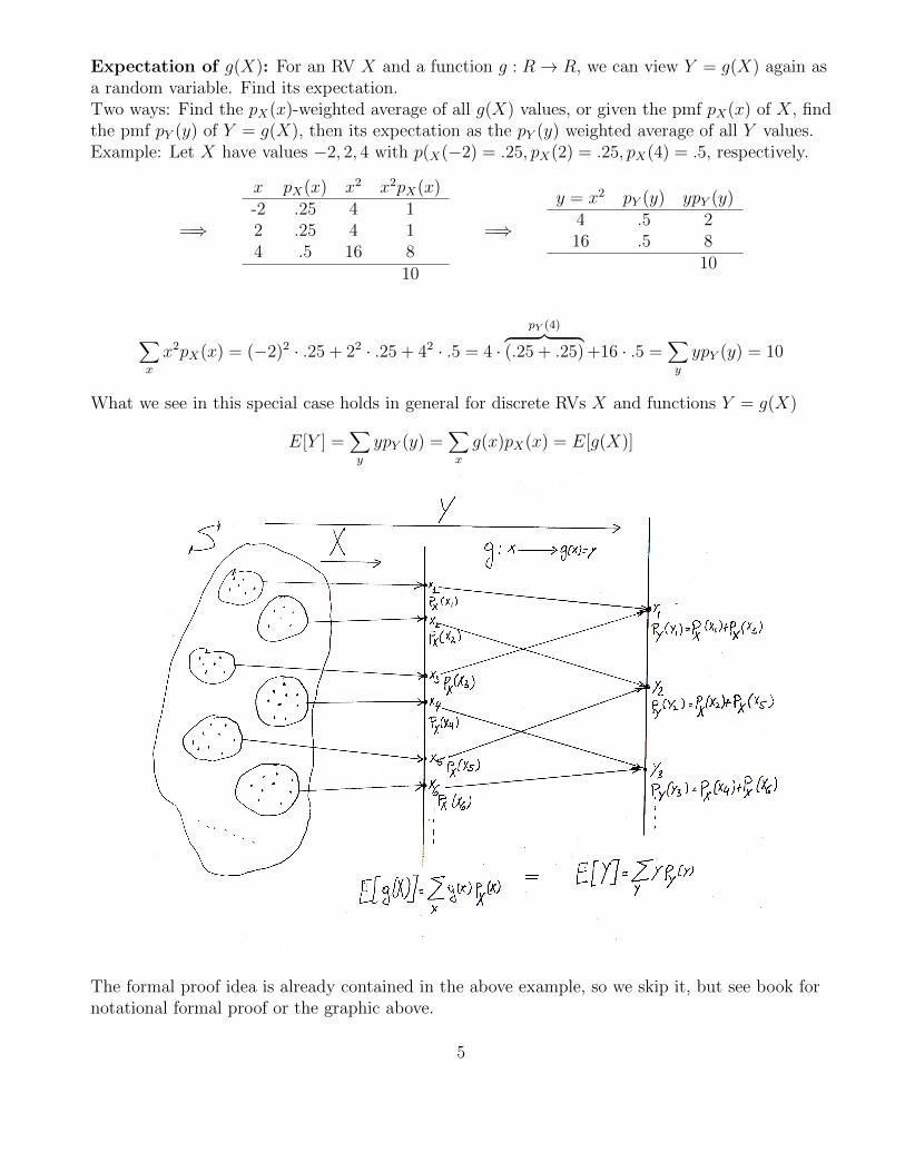
gene d dominates over the recessive r, i.e., the trait shows whenever there is a d in the gene pair.An offspring from two parents inherits randomly one gene from each gene pair of its parents. Ifboth parents are hybrids ({d, r}) what is the chance that of 4 offspring at least 3 show theoutward appearance of the dominant gene?Solution: p = 3/4 is the probability that any given offspring will have gene pair {d, d} or {d, r}.Hence P = 4(3/4)3(1/4) + 1(3/4)4 = 189/256 = .74.Example 18 (Reliability): On an aircraft we want to compare the reliability (probability offunctioning) of a 3 out of 5 system with a 2 out of 3 system. A k out of n system functionswhenever a majority of the subsystems function properly. Usually n is chosen as odd. We assumethat the probability of failure 1− p is the same all subsystems and that failures occurindependently. A 3 out of 5 system has a higher reliability than a 2 out of 3 system whenever(

5

3

)p3(1−p)2+

(5

4

)p4(1−p)+

(5

5

)p5 >

(3

2

)p2(1−p)+

(3

3

)p3 ⇐⇒ (1−p)(2p−1) > 0 ⇐⇒ p >

1

2

0.0 0.2 0.4 0.6 0.8 1.0

0.0

0.4

0.8

p

relia

bilit

y

3 out of 5 system2 out of 3 system

0.95 0.96 0.97 0.98 0.99 1.00

0.99

880.

9994

1.00

00

p

relia

bilit

y

3 out of 5 system2 out of 3 system

9

Mean and Variance of X ∼ Bin(n, p): Using the simple identities

i

(n

i

)= n

(n− 1

i− 1

)and i(i− 1)

(n

i

)= n(n− 1)

(n− 2

i− 2

)

=⇒ E[X] =n∑i=0

i

(n

i

)pi(1− p)n−i =

n∑i=1

np

(n− 1

i− 1

)pi−1(1− p)n−1−(i−1)

substituting i− 1 = j = npn−1∑j=0

(n− 1

j

)pj(1− p)n−1−j = np

Note the connection to Bernoulli RVs Xi, indicating success or failure in the ith trial andE[X] = E[X1 + . . .+Xn] = E[X1] + . . .+ E[Xn] = np.Expectation of a sum = sum of the individual (finite) expectations.

E[X(X − 1)] =n∑i=0

i(i− 1)

(n

i

)pi(1− p)n−i =

n∑i=2

n(n− 1)p2(n− 2

i− 2

)pi−2(1− p)n−2−(i−2)

substituting i− 2 = j = n(n− 1)p2n−2∑j=0

(n− 2

j

)pj(1− p)n−2−j = n(n− 1)p2

n(n− 1)p2 = E[X(X − 1)] = E[X2 −X] =∑x

(x2 − x)p(x) =∑x

x2p(x)−∑x

xp(x)

= E[X2]− E[X] = E[X2]− np=⇒ E[X2] = np+ n(n− 1)p2 = np(1− p) + (np)2

=⇒ var(X) = E[X2]− (E[X])2 = np(1− p)

Note again var(X) = var(X1 + . . .+Xn) = var(X1) + . . .+ var(Xn) = np(1− p)

Variance of a sum of independent RVs = sum of the (finite) variances of those RVs.Qualitative Behavior of Binomial Probability Mass Function: If X is a binomial randomvariable with parameters (n, p) then the probability mass function p(x) of X first increasesmonotonically and then decreases monotonically, reaching its largest value when x is the largestinteger ≤ (n+ 1)p.Proof: Look at p(x+ 1)/p(x) = p

1−pn−xx+1

> 1 or < 1 ⇐⇒ (n+ 1)p > x+ 1 or < x+ 1. Of course it

is possible that p(x) is entirely monotone (when?). Illustrate with Pascal’s triangle. L16ends

The Poisson Random Variable

Definition: A random variable X with possible values 0, 1, 2, . . . is called a Poisson randomvariable, indicated by X ∼ Pois(λ), if for some constant λ > 0 its pmf is given by

p(i) = P (X = i) = P (Pois(λ) = i) = e−λλi

i!for i = 0, 1, 2, . . . .3 Check summation to 1.

3In R get p(i) = P (X = i) via the command dpois(i,lambda), while P (X ≤ i) is obtained by ppois(i,lambda).In EXCEL you get the same by =POISSON(i,lambda,FALSE) and =POISSON(i,lambda,TRUE), respectively.

10

Approximation to a binomial random variable for small p and large n: Let X be abinomial rv with parameters n and p. Let n get large and let p get small so that λ = np doesneither degenerate to 0 nor ∞, then

P (X = i) =n!

i!(n− i)pi(1− p)n−i =

n!

i!(n− i)!

(λ

n

)i (1− λ

n

)n−i

=n(n− 1) · · · (n− i+ 1)

niλi

i!

(1− λ/n)n

(1− λ/n)i≈ e−λ

λi

i!.

Since np represents the expected or average number of successes of the n trials represented by thebinomial random variable it should not be surprising that the Poisson prameter λ should beinterpreted as the average or expected count for such a Poisson random variable.Actually, for the approximation to work it can be shown that small p is sufficient. In fact, if fori = 1, 2, 3, . . . , n the Xi are independent Bernoulli random variables with respective successprobabilities pi and if S = X1 + · · ·+Xn and if Y is a Poisson random variable with parameterλ =

∑ni=1 pi then

|P (S ≤ x)− P (Y ≤ x)| ≤ 3(max(p1, . . . , pn))1/3 for all x

or one can show that

|P (S ≤ x)− P (Y ≤ x)| ≤ 2n∑i=1

p2i for all x .

Poisson-Binomial Approximation, see class web page.A Poisson random variable often serves as a good model for the count of rare events.Examples:Number of misprints on a pageNumber of telephone calls coming through an exchangeNumber of wrong numbers dialedNumber of lightning strikes on commercial aircraftNumber of bird ingestions into the engine of a jetNumber of engine failures on a jetNumber of customers coming into a post office on a given dayNumber of meteoroids striking an orbiting space stationNumber of discharged α–particles from some radioactive source.Example 19: (Typos): Let X be the number of typos on a single page of a given book.Assume that X is Poisson with parameter λ = .5, i.e. we expect about half an error per page orabout one error per every two pages. Find the probability of at least one error. Solution:P (X ≥ 1) = 1− P (X = 0) = 1− exp(−.5) = .393.Example 20 (Defectives): A machine produces 10% defective items, i.e. an item coming offthe machine has a chance of .1 of being defective. What is the chance that in the next 10 itemscoming off the machine we find at most one defective item? Solution: Let X be the number ofdefective items among the 10.

P (X ≤ 1) = P (X = 0) + P (X = 1) = (.1)0(.9)10 + 10(.1)1(.9)9 = .7361

whereas using a Poisson random variable Y with parameter λ = 10(.1) = 1 we get

P (Y ≤ 1) = P (Y = 0) + P (Y = 1) = e−1 + e−1 = .7358

11

Mean and Variance of the Poisson Distribution: Based on the approximation of theBinomial(n, p) by a Poisson(λ = np) distribution when p is small, we would expect thatE[Y ] ≈ np = λ and var(Y ) ≈ np(1− p) ≈ λ. We now show that these approximations are in factexact.

E[Y ] =∞∑i=0

ie−λλi

i!= λ

∞∑i=1

e−λλi−1

(i− 1)!= λ

∞∑j=0

e−λλj

j!= λ

L17endsE[Y 2] =

∞∑i=0

i2e−λλi

i!= λ

∞∑i=1

ie−λλi−1

(i− 1)!= λ

∞∑j=0

(j + 1)e−λλj

j!= λ

∞∑j=0

je−λλj

j!+ λ

∞∑j=0

e−λλj

j!= λ2 + λ

=⇒ var(Y ) = E[Y 2]− (E[Y ])2 = λ2 + λ− λ2 = λ

Poisson Distribution for Events in Time (Another Justification): Sometimes we observerandom incidents occurring in time, e.g. arrival of customers, meteoroids, lightning etc. Quiteoften these random phenomena appear to satisfy the following basic assumptions for somepositive constant λ:

1. The probability that exactly one incident occurs during an interval of length h is λh+ o(h)where o(h) is a function of h which goes to 0 faster than h, i.e. o(h)/h→ 0 as h→ 0 (e.g.o(h) = h2). The concept/notation of o(h) was introduced by Edmund Landau.

2. The probability that two or more incidents occur in an interval of length h is the same forall such intervals and equal to o(h). No clustering of incidents!

3. For any integers n, j1, . . ., jn and any set of nonoverlapping intervals the events E1, . . ., En,with Ei denoting the occurrence of exactly ji incidents in the ith interval, are independent.

If N(t) denotes the number of incidents in a given interval of length t then it can be shown thatN(t) is a Poisson random variable with parameter λt, i.e. P (N(t) = k) = e−λt(λt)k/k!.Proof: Take as time interval [0, t] and divide it into n equal parts. P (N(t) = k) = P (k of theintervals contain exactly one incident and n− k contain 0 incidents)+P (N(t) = k and at leastone subinterval contains two or more incidents). The second probability can be bounded by

n∑i=1

P (ith interval contains at least two incidents) ≤n∑i=1

o(t

n

)= n o(t/n)→ 0 .

The probability of 0 incidents in a particular interval of length t/n is 1− [λ(t/n) + o(t/n)] so thatthe first probability above becomes (in cavalier fashion, not quite air tight. See Poisson-BinomialApproximation on the class web page for a clean argument.)

n!

k!(n− k)!

[λt

n+ o(t/n)

]k [1− λt

n− o(t/n)

]n−kwhich converges to exp(−λt)(λt)k/k!.Example 21 (Space Debris): It is estimated that the space station will be hit by space debrisbeyond a critical size and velocity on the average about once in 500 years. What is the chancethat the station will survive the first 20 years without such a hit.Solution: T = 500 then λT = 1 or λ = 1/500. Now t = 20 andP (N(t) = 0) = exp(−λt) = exp(−20/500) = .9608.

12

Geometric, Negative Binomial and HypergeometricRandom Variables

Definition: In independent trials with success probability p the number X of trials required toget the first success is called a geometric random variable. We write X ∼ Geo(p) to indicate itsdistribution. Its probability mass function is

p(n) = P (X = n) = P (Geo(p) = n) = (1− p)n−1p for n = 1, 2, 3, . . .

Check summation to 1. Some texts (and software, e.g., R and EXCEL as a special negativebinomial) treat X0 = X − 1 = number of failures before the first success as the geometric RV.Then P (X0 = n) = P (X = n+ 1) = (1− p)np for n = 0, 1, 2, . . ..Example 22 (Urn Problem): An urn contains N white and M black balls. Balls are drawnwith replacement until the first black ball is obtained. Find P (X = n) and P (X ≥ k), the latterin two ways. Probability of success = p = M/(M +N).

P (X = n) = (1− p)n−1p and P (X ≥ k) = (1− p)k−1

P (X ≥ k) =∞∑i=k

(1− p)i−1p = (1− p)k−1∞∑i=k

(1− p)i−kp

= p(1− p)k−1∞∑j=0

(1− p)j = p(1− p)k−1 1

1− (1− p)= (1− p)k−1

Mean and Variance of X ∼ Geo(p):

E[X]− 1 = E[X − 1] =∞∑n=1

(n− 1)(1− p)n−1p = (1− p)∞∑n=2

(n− 1)(1− p)n−2p

= (1− p)∞∑i=1

i(1− p)i−1p = (1− p)E[X] =⇒ E[X](1− (1− p)) = 1 or E[X] =1

p

Fits intuition: If p = 1/1000, then it takes on average 1/p = 1000 trials to see one success. L18ends

E[X2]− 2E[X] + 1 = E[(X − 1)2] =∞∑n=1

(n− 1)2(1− p)n−1p = (1− p)∞∑n=2

(n− 1)2(1− p)n−2p

= (1− p)∞∑i=1

i2(1− p)i−1p = (1− p)E[X2]

=⇒ E[X2](1− (1− p)) =2

p− 1 or E[X2] =

2

p2− 1

p

or var(X) = E[X2]− (E[X])2 =2

p2− 1

p− 1

p2=

1− pp2

Definition: In independent trials with success probability p the number X of trials required toget the first r successes accumulated is called a negative binomial random variable. We writeX ∼ NegBin(r, p) to indicate its distribution. Its probability mass function is

p(n) = P (X = n) = P (NegBin(r, p) = n) =

(n− 1

r − 1

)(1− p)n−rpr for n = r, r + 1, r + 2, . . .

13

For r = 1 we get the geometric distribution as a special case.Exploiting the equivalence of the two statements:“it takes at least m trials to get r successes” and“in the first m− 1 trials we have at most r − 1 successes” we have

P (NegBin(r, p) ≥ m) = 1− P (NegBin(r, p) ≤ m− 1) = P (Bin(m− 1, p) ≤ r − 1) (1)

This facilitates the computation of the negative binomial cumulative probabilities in terms ofappropriate binomial cumulative probabilities.We can view X as the sum of independent geometric random variables Y1, . . . , Yr, each withsuccess probability p. Here Y1 denotes the number of trials to the first succes, Y2 the number ofadditional trials to the next success thereafter, and so on. Clearly, for i1, . . . , ir ∈ {1, 2, 3, . . .} wehave

P (Y1 = i1, . . . , Yr = ir) = P (Y1 = i1) · . . . · P (Yr = ir) (2)

since the individual statements concern what specifically happens in the first i1 + . . .+ ir trials,all of which are independent, namely we have i1 − 1 failures, then a success, then i2 − 1 failures,then a success, and so on. From (2) it follows that for E1, . . . , Er ⊂ {1, 2, 3, . . .} we have

P (Y1 ∈ E1, . . . , Yr ∈ Er) =∑i1∈E1

. . .∑ir∈Er

P (Y1 = i1, . . . , Yr = ir)

=∑i1∈E1

. . .∑ir∈Er

P (Y1 = i1) · . . . · P (Yr = ir)

distributive law of arithmetic =∑i1∈E1

P (Y1 = i1) · . . . ·∑ir∈Er

P (Yr = ir)

= P (Y1 ∈ E1) · . . . · P (Yr ∈ Er)

The same holds for any subset of the Y1, . . . , Yr, since (2) also holds for any subset. For example,summing the left and right side over all i1 = 1, 2, 3, . . . yields

∞∑i1=1

P (Y1 = i1, . . . , Yr = ir) =∞∑i1=1

P (Y1 = i1) · . . . · P (Yr = ir)

P (Y1 <∞, Y2 = i2, . . . , Yr = ir) = P (Y1 <∞) · P (Y2 = i2) · . . . · P (Yr = ir)

P (Y2 = i2, . . . , Yr = ir) = P (Y2 = i2) · . . . · P (Yr = ir)

and similarly by summing over any other and further indices. In particular we get

1 = P (Y1 <∞) · . . . ·P (Yr <∞) = P (Y1 <∞, . . . , Yr <∞) ≤ P (Y1 + . . .+Yr <∞) = P (X <∞)

This means that the negative binomial pmf sums to 1, i.e.,

1 = P (X <∞) =∞∑n=r

P (X = n) =∞∑n=r

(n− 1

r − 1

)(1− p)n−rpr

Some texts (and software such as R and EXCEL) treat X0 = X − r = number of failures prior to L19endsthe rth success as a negative binomial RV. Then P (X0 = n) = P (X = n+ r) for n = 0, 1, 2, . . .4.

4P (X0 = n) and P (X0 ≤ n) can be obtained in R by the commands dnbinom(n,r,p) and pnbinom(n,r,p),respectively, while in EXCEL use = NEGBINOMDIST(n,r,p) and =1-BINOMDIST(r-1,n+r,p,TRUE) based on (1).E.g., pnbinom(4,5,.2) and =1-BINOMDIST(4,9,0.2,TRUE) return 0.01958144.

14

Example 23 (r Successes Before m Failures): If independent trials are performed withsuccess probability p what is the chance of getting r successes before m failures?Solution: Let X be the number of trials required to get the first r successes. Then we need tofind: P (X ≤ m+ r − 1) = P (X0 ≤ m− 1).

Mean and Variance of X ∼ NegBin(r, p): Using n(n−1r−1

)= r

(nr

)and V ∼ NegBin(r + 1, p)

E[Xk] =∞∑n=r

nk(n− 1

r − 1

)pr(1− p)n−r =

r

p

∞∑n=r

nk−1(n

r

)pr+1(1− p)n−r

=r

p

∞∑n+1=r+1

(n+ 1− 1)k−1(n+ 1− 1

r + 1− 1

)pr+1(1− p)n+1−(r+1)

=r

p

∞∑m=r+1

(m− 1)k−1(

m− 1

r + 1− 1

)pr+1(1− p)m−(r+1) =

r

pE[(V − 1)k−1]

=⇒ E[X] = rp

and

E[X2] =r

pE[V − 1] =

r

p

(r + 1

p− 1

)=⇒ var(X) =

r

p

r + 1

p− r

p−(r

p

)2

=r(1− p)p2

If we write X again as X = Y1 + . . .+Yr with independent Yi ∼ Geo(p), i = 1, . . . , r, we note again

E[X] = E[Y1 + . . .+ Yr] = E[Y1] + . . .+ E[Yr] =r

p

var(X) = var(Y1 + . . .+ Yr) = var(Y1) + . . .+ var(Yr) = r1− pp2

Definition: If a sample of size n is chosen randomly and without replacement from an urncontaining N balls, of which M = Np are white and N −M = N −Np are black, then thenumber X of white balls in the sample is called a hypergeometric random variable. To indicateits distribution we write X ∼ Hyper(n,M,N). Its possible values are x = 0, 1, . . . , n with pmf

p(k) = P (X = k) =

(Mk

)(N−Mn−k

)(Nn

) (3)

which is positive only if 0 ≤ k and k ≤M and 0 ≤ n− k and n− k ≤ N −M , i.e. ifmax(0, n−N +M) ≤ k ≤ min(n,M).5

Expression (3) also applies when drawing the n balls one by one without replacement since then

P (X = k) =

(nk

)M(M − 1) . . . (M − k + 1)(N −M)(N −M − 1) . . . (N −M − (n− k + 1))

N(N − 1) . . . (N − n+ 1)

=

(Mk

)(N−Mn−k

)(Nn

)5In R we can obtain P (X = k) and P (X ≤ k) by the commands dhyper(k,M,N-M,n) and phyper(k,M,N-M,n),

respectively. EXCEL only gives P (X = k) directly via =HYPGEOMDIST(k,n,M,N). For example, for M = 40, N =100, n = 30 and k = 15 dhyper(15,40,60,30) and =HYPGEOMDIST(15,30,40,100) return P (X = 15) = .07284917,while phyper(15,40,60,30) returns P (X ≤ 15) = .9399093.

15

Example 24 (Animal Counts): r animals are caught and tagged and released. After areasonable time interval n animals are captured and the number X of tagged ones are counted.The total number N of animals is unknown. Then

pN(i) = P (X = i) =

(ri

)(N−rn−i

)(Nn

)Find N which maximizes this pN(i) for the observed value X = i.

pN(i)

pN−1(i)=

(N − r)(N − n)

N(N − r − n+ i)≥ 1

if and only if N ≤ rn/i. Hence our maximum likelihood estimate is N̂ = largest integer ≤ rn/i.Another way of motivating this estimate is to appeal to r/N ∼ i/n.Example 25 (Quality Control): Shipments of 1000 items each are inspected by selecting 10without replacement. If the sample contains more than one defective then the whole shipment isrejected. What is the chance for rejecting a shipment if at most 5% of the shipment is bad. Theprobability of no rejection is

P (X = 0) + P (X = 1) =

(500

)(95010

)(100010

) +

(501

)(9509

)(100010

) = .91469

hence the chance of rejecting a shipment is at most .08531.

Expections and Variances of X1 + . . .+Xn:First we prove a basic alternate formula for the expectation of a single random variable X:

E[X] =∑x

xpX(x) =∑s

X(s)p(s)

where the first expression involves the pmf pX(x) ofX and sums over all possible values ofX and thesecond expression involves the probability p(s) = P ({s}) for all elements s in the sample space S.The equivalence is seen as follows. For any of the possible values x ofX let Sx = {s ∈ S : X(s) = x}.For different values x the events/sets Sx are disjoint and their union over all x is S. Thus∑

x

xpX(x) =∑x

xP ({s : X(s) = x}) =∑x

x∑s∈Sx

p(s)

=∑x

∑s∈Sx

xp(s) =∑x

∑s∈Sx

X(s)p(s) =∑s

X(s)p(s)

From this we get immediately

E[X1 + . . .+Xn] =∑s

(X1(s) + . . .+Xn(s))p(s) =∑s

[X1(s)p(s) + . . .+Xn(s)p(s)]

=∑s

X1(s)p(s) + . . .+∑s

Xn(s)p(s) = E[X1] + . . .+ E[X2]

provided the individual expectations are finite.

16

Next we will we address a corresponding formula for the variance of a sum of independent discreterandom variables X1, . . . , Xn, namely

var(X1 + . . .+Xn) = var(X1) + . . .+ var(Xn) provided the individual variances are finite.

First we need to define the concept independence for a pair of random variables X and Y inconcordance with the previously introduced independence of events. X and Y are independent,whenever for all possible values x and y of X and Y we have

P (X = x, Y = y) = P ({s ∈ S : X(s) = x, Y (s) = y})= P ({s ∈ S : X(s) = x})P ({s ∈ S : Y (s) = y}) = P (X = x)P (Y = y)

As a consequence we have for independent X and Y with finite expectations the following property

E[XY ] = E[X]E[Y ] , i.e., E[XY ]− E[X]E[Y ] = cov(X, Y ) = 0

where cov(X, Y ) is the covariance of X and Y , equivalently defined as

cov(X, Y ) = E[(X − E[X])(Y − E[Y ])] = E[XY −XE[Y ]− Y E[X] + E[X]E[Y ]]

= E[XY ]− E[X]E[Y ]− E[X]E[Y ] + E[X]E[Y ] = E[XY ]− E[X]E[Y ]

Proof of independence =⇒ cov(X, Y ) = 0: Let Sxy = {s ∈ S : X(s) = x, Y (s) = y}

E[XY ] =∑s

X(s)Y (s)p(s) =∑x,y

∑s∈Sxy

X(s)Y (s)p(s) by stepwise summation

=∑x,y

∑s∈Sxy

xyp(s) =∑x,y

xy∑s∈Sxy

p(s) by distributive law

=∑x,y

xyP (X = x, Y = y) =∑x,y

xyP (X = x)P (Y = y) by independence

by distributive law =∑x

xP (X = x)∑y

yP (Y = y) = E[X]E[Y ]

E[(X1 + . . .+Xn)2

]= E

n∑i=1

X2i + 2

n∑i<j

XiXj

=n∑i=1

E[X2i

]+ 2

n∑i<j

E [XiXj]

=n∑i=1

E[X2i

]+ 2

n∑i<j

E[Xi]E[Xj]

(E[X1 + . . .+Xn])2 = (E[X1] + . . .+ E[Xn])2 =n∑i=1

(E[Xi])2 + 2

n∑i<j

E[Xi]E[Xj]

var(X1 + . . .+Xn) = E[(X1 + . . .+Xn)2

]− (E[X1 + . . .+Xn])2

=n∑i=1

(E[X2

i ]− (E[Xi])2)

+ 2n∑i<j

(E [XiXj]− E[Xi]E[Xj])

=n∑i=1

var(Xi) + 2n∑i<j

cov(Xi, Xj) =n∑i=1

var(Xi)

where the last = holds for pairwise independence of Xi and Xj for i < j.

17

The above rules for mean and variance of Y = X1 + . . .+Xn are now illustrated for two situations.Let X1, . . . , Xn be indicator RVs indicating a success or failure in the ith of n trials. In the firstsituation we assume these trials are independent and have success probability p each. Then, asobserved previously, from the mean and variance results for Bernoulli RVs we get

E[Y ] = E(X1+. . .+Xn) =n∑i=1

E[Xi] = np and var(Y ) = var(X1+. . .+Xn) =n∑i=1

var(Xi) = np(1−p)

In the second situation we view the trials in the hypergeometric context, where Xi = 1 when theith ball drawn is white and Xi = 0 otherwise. We argued previously that P (Xi = 1) = M/N = p =proportion of white balls in the population

=⇒ E[Y ] = E(X1 + . . .+Xn) =n∑i=1

E[Xi] =nM

N

For var(Y ) we need to involve the covariance terms in our formula for var(X1 + . . .+Xn). We find

E[XiXj] = P (Xi = 1, Xj = 1) =M(M − 1)(N − 2) . . . (N − n+ 1)

N(N − 1)(N − 2) . . . (N − n+ 1)=M(M − 1)

N(N − 1)

cov(Xi, Xj) = E[XiXj]− E[Xi]E[Xj] =M(M − 1)

N(N − 1)− M

N

M

N= −M

N

N −MN(N − 1)

= −p(1− p)N − 1

var(Y ) = var(X1 + . . .+Xn) =n∑i=1

var(Xi) + 2n∑i<j

cov(Xi, Xj)

= np(1− p)− 2

(n

2

)p(1− p)N − 1

= np(1− p)(

1− n− 1

N − 1

)= np(1− p)N − n

N − 1

The factor 1− (n− 1)/(N − 1) is called the finite population correction factor. For fixed n itgets close to 1 when N is large, in which case it does not matter much whether we draw with orwithout replacement. One easily shows (exercise, or see Text p. 162) that

P (Hyper(n,M,N) = k) −→ P (Bin(n, p) = k) =

(n

k

)pk(1−p)n−k as N −→∞, where p = M/N

We will now pull forward material from Ch. 8, namely the inequalities of Markov and Chebychev6.Markov’s Inequality: Let X be a nonnegative discrete RV with finite expectation E[X] then forany a > 0 we have

P (X ≥ a) ≤ E[X]

a

Proof: E[X] =∑x≥a

xpX(x)+∑x<a

xpX(x) ≥∑x≥a

xpX(x) ≥∑x≥a

apX(x) = aP (X ≥ a)

Markov’s inequality is only meaningful for a > E[X]. It limits the probability far beyond the meanor expectation of X, in concordance with our previous center of gravity interpretation of E[X].

6Scholz ← Lehmann ← Neyman ← Sierpinsky ← Voronoy ← Markov ← Chebychev

18

While this inequality is usually quite crude, it can be sharp, i.e., result in equality. Namely, let Xtake the two values 0 and a with probability 1− p and p. Then p = P (X ≥ a) = E[X]/a.Chebychev’s Inequality: Let X be a discrete RV with finite variance E[(X − µ)2] = σ2, thenfor any k > 0 we have

P (|X − µ| ≥ k) ≤ σ2

k2

Proof by Markov’s inequality using Y = (X − µ)2 as our nonnegative RV

P (|X − µ| ≥ k) = P ((X − µ)2 ≥ k2) ≤ E[(X − µ)2]

k2=σ2

k2

These inequalities hold also for RVs that are not discrete, but why wait that long for the following.We will now combine the above results into a theorem that proves the long run frequency notionthat we have alluded to repeatedly, in particular when introducing the axioms of probability.Let X̄ = (X1 + . . . + Xn)/n be the average of n independent and identically distributed randomvariables (telegraphically expressed as iid RVs), each with same mean µ = E[Xi] and varianceσ2 = var(Xi). Such random variables can be the result of repeatedly observing a random variableX in independent repetitions of the same random experiment, like repeatedly tossing a coin orrolling a die, and denoting the resulting RVs by X1, . . . , Xn.Using the rules of expectation and variance (under independence) we have

E[X̄] =1

nE[X1 + . . .+Xn] =

1

n(µ+ . . .+ µ) = µ

var(X̄) =1

n2var(X1 + . . .+Xn) =

1

n2(σ2 + . . .+ σ2) =

σ2

n

and by Chebychev’s inequality applied to X̄ we get for any ε > 0

P (|X̄ − µ| ≥ ε) ≤ σ2

n

1

ε2−→ 0 as n −→∞,

i.e., the probability that X̄ will differ from µ by at least ε > 0 becomes vanishingly small.

We say X̄ converges to µ in probability and write X̄P−→ µ as n −→∞.

This result is called the weak law of large numbers (WLLN or LLN without emphasis on weak).When our random experiment consists of observing whether a certain event E occurs or not, weobserve an indicator variable X = IE with values 1 and 0. If we repeatedly do this experiment(independently), we observe X1, . . . , Xn, each with mean µ = p = P (E) and variance σ2 = p(1−p).In that case X̄ is the proportion of 1’s among theX1, . . . , Xn, i.e., the proportion of times we observethe event E.The above law of large numbers gives us X̄

P−→ µ = p = P (E) as n −→ ∞, i.e., in the long runthe observed proportion or relative frequency of observing the event E converges to P (E).

19

Properties of Distribution Functions F :

1. F is nondecreasing, i.e. F (a) ≤ F (b) for a, b with a ≤ b.

2. limb→∞ F (b) = 1

3. limb→−∞ F (b) = 0

4. F is right continuous, i.e. if bn ↓ b then F (bn) ↓ F (b) or limn→∞ F (bn) = F (b).

Proof:1. For a ≤ b we have {e : X(e) ≤ a} ⊂ {e : X(e) ≤ b}.2., 3. and 4. ⇐= P (limn→∞En) = limn→∞ P (En) for properly chosen monotone sequences En.E.g., if bn ↓ b then En = {e : X(e) ≤ bn} ↘ E = {e : X(e) ≤ b} =

⋂∞n=1En

All probability questions about X can be answered in terms of the cdf F of X. For example,

• P (a < X ≤ b) = F (b)− F (a) for all a ≤ b

• P (X < b) = limn→∞ F (b− 1n) =: F (b−)

• F (b) = P (X ≤ b) = P (X < b) + P (X = b) = F (b−) + (F (b)− F (b−))

20