Embed Size (px)
Citation preview

LECTURE NOTES ON
GAS DYNAMICS
Joseph M. Powers
Department of Aerospace and Mechanical Engineering
University of Notre DameNotre Dame, Indiana 46556-5637
USA
updated
17 February 2015, 7:48am

Contents
Preface 7
1 Introduction 91.1 Definitions . . . . . . . . . . . . . . . . . . . . . . . . . . . . . . . . . . . . . 91.2 Motivating examples . . . . . . . . . . . . . . . . . . . . . . . . . . . . . . . 10
1.2.1 Re-entry flows . . . . . . . . . . . . . . . . . . . . . . . . . . . . . . . 101.2.1.1 Bow shock wave . . . . . . . . . . . . . . . . . . . . . . . . 101.2.1.2 Rarefaction (expansion) wave . . . . . . . . . . . . . . . . . 111.2.1.3 Momentum boundary layer . . . . . . . . . . . . . . . . . . 111.2.1.4 Thermal boundary layer . . . . . . . . . . . . . . . . . . . . 121.2.1.5 Vibrational relaxation effects . . . . . . . . . . . . . . . . . 121.2.1.6 Dissociation effects . . . . . . . . . . . . . . . . . . . . . . . 12
1.2.2 Rocket nozzle flows . . . . . . . . . . . . . . . . . . . . . . . . . . . . 121.2.3 Jet engine inlets . . . . . . . . . . . . . . . . . . . . . . . . . . . . . . 13
2 Governing equations 152.1 Mathematical preliminaries . . . . . . . . . . . . . . . . . . . . . . . . . . . 15
2.1.1 Vectors and tensors . . . . . . . . . . . . . . . . . . . . . . . . . . . . 152.1.2 Gradient, divergence, and material derivatives . . . . . . . . . . . . . 162.1.3 Conservative and non-conservative forms . . . . . . . . . . . . . . . . 17
2.1.3.1 Conservative form . . . . . . . . . . . . . . . . . . . . . . . 172.1.3.2 Non-conservative form . . . . . . . . . . . . . . . . . . . . . 17
2.2 Summary of full set of compressible viscous equations . . . . . . . . . . . . . 202.3 Conservation axioms . . . . . . . . . . . . . . . . . . . . . . . . . . . . . . . 21
2.3.1 Conservation of mass . . . . . . . . . . . . . . . . . . . . . . . . . . . 222.3.1.1 Nonconservative form . . . . . . . . . . . . . . . . . . . . . 222.3.1.2 Conservative form . . . . . . . . . . . . . . . . . . . . . . . 222.3.1.3 Incompressible form . . . . . . . . . . . . . . . . . . . . . . 22
2.3.2 Conservation of linear momenta . . . . . . . . . . . . . . . . . . . . . 222.3.2.1 Nonconservative form . . . . . . . . . . . . . . . . . . . . . 222.3.2.2 Conservative form . . . . . . . . . . . . . . . . . . . . . . . 23
2.3.3 Conservation of energy . . . . . . . . . . . . . . . . . . . . . . . . . . 24
3

4 CONTENTS
2.3.3.1 Nonconservative form . . . . . . . . . . . . . . . . . . . . . 242.3.3.2 Mechanical energy . . . . . . . . . . . . . . . . . . . . . . . 252.3.3.3 Conservative form . . . . . . . . . . . . . . . . . . . . . . . 252.3.3.4 Energy equation in terms of entropy . . . . . . . . . . . . . 26
2.3.4 Entropy inequality . . . . . . . . . . . . . . . . . . . . . . . . . . . . 262.4 Constitutive relations . . . . . . . . . . . . . . . . . . . . . . . . . . . . . . . 29
2.4.1 Stress-strain rate relationship for Newtonian fluids . . . . . . . . . . . 292.4.2 Fourier’s law for heat conduction . . . . . . . . . . . . . . . . . . . . 332.4.3 Variable first coefficient of viscosity, µ . . . . . . . . . . . . . . . . . . 34
2.4.3.1 Typical values of µ for air and water . . . . . . . . . . . . . 342.4.3.2 Common models for µ . . . . . . . . . . . . . . . . . . . . . 35
2.4.4 Variable second coefficient of viscosity, λ . . . . . . . . . . . . . . . . 352.4.5 Variable thermal conductivity, k . . . . . . . . . . . . . . . . . . . . . 35
2.4.5.1 Typical values of k for air and water . . . . . . . . . . . . . 352.4.5.2 Common models for k . . . . . . . . . . . . . . . . . . . . . 36
2.4.6 Thermal equation of state . . . . . . . . . . . . . . . . . . . . . . . . 362.4.6.1 Description . . . . . . . . . . . . . . . . . . . . . . . . . . . 362.4.6.2 Typical models . . . . . . . . . . . . . . . . . . . . . . . . . 36
2.4.7 Caloric equation of state . . . . . . . . . . . . . . . . . . . . . . . . . 362.4.7.1 Description . . . . . . . . . . . . . . . . . . . . . . . . . . . 362.4.7.2 Typical models . . . . . . . . . . . . . . . . . . . . . . . . . 37
2.5 Special cases of governing equations . . . . . . . . . . . . . . . . . . . . . . . 372.5.1 One-dimensional equations . . . . . . . . . . . . . . . . . . . . . . . . 372.5.2 Euler equations . . . . . . . . . . . . . . . . . . . . . . . . . . . . . . 382.5.3 Incompressible Navier-Stokes equations . . . . . . . . . . . . . . . . . 38
3 Thermodynamics review 393.1 Preliminary mathematical concepts . . . . . . . . . . . . . . . . . . . . . . . 393.2 Summary of thermodynamic concepts . . . . . . . . . . . . . . . . . . . . . . 403.3 Maxwell relations and secondary properties . . . . . . . . . . . . . . . . . . . 44
3.3.1 Internal energy from thermal equation of state . . . . . . . . . . . . . 453.3.2 Sound speed from thermal equation of state . . . . . . . . . . . . . . 47
3.4 Canonical equations of state . . . . . . . . . . . . . . . . . . . . . . . . . . . 533.5 Isentropic relations . . . . . . . . . . . . . . . . . . . . . . . . . . . . . . . . 55
4 One-dimensional compressible flow 614.1 Generalized one-dimensional equations . . . . . . . . . . . . . . . . . . . . . 62
4.1.1 Mass . . . . . . . . . . . . . . . . . . . . . . . . . . . . . . . . . . . . 634.1.2 Momentum . . . . . . . . . . . . . . . . . . . . . . . . . . . . . . . . 634.1.3 Energy . . . . . . . . . . . . . . . . . . . . . . . . . . . . . . . . . . . 654.1.4 Influence coefficients . . . . . . . . . . . . . . . . . . . . . . . . . . . 72
4.2 Flow with area change . . . . . . . . . . . . . . . . . . . . . . . . . . . . . . 73
CC BY-NC-ND. 17 February 2015, J. M. Powers.

CONTENTS 5
4.2.1 Isentropic Mach number relations . . . . . . . . . . . . . . . . . . . . 73
4.2.2 Sonic properties . . . . . . . . . . . . . . . . . . . . . . . . . . . . . . 81
4.2.3 Effect of area change . . . . . . . . . . . . . . . . . . . . . . . . . . . 82
4.2.4 Choking . . . . . . . . . . . . . . . . . . . . . . . . . . . . . . . . . . 84
4.3 Normal shock waves . . . . . . . . . . . . . . . . . . . . . . . . . . . . . . . 87
4.3.1 Governing equations . . . . . . . . . . . . . . . . . . . . . . . . . . . 88
4.3.2 Rayleigh line . . . . . . . . . . . . . . . . . . . . . . . . . . . . . . . 89
4.3.3 Hugoniot curve . . . . . . . . . . . . . . . . . . . . . . . . . . . . . . 89
4.3.4 Solution procedure for general equations of state . . . . . . . . . . . 91
4.3.5 Calorically perfect ideal gas solutions . . . . . . . . . . . . . . . . . . 91
4.3.6 Acoustic limit . . . . . . . . . . . . . . . . . . . . . . . . . . . . . . . 102
4.3.7 Non-ideal gas solutions . . . . . . . . . . . . . . . . . . . . . . . . . . 103
4.4 Flow with area change and normal shocks . . . . . . . . . . . . . . . . . . . 107
4.4.1 Converging nozzle . . . . . . . . . . . . . . . . . . . . . . . . . . . . . 107
4.4.2 Converging-diverging nozzle . . . . . . . . . . . . . . . . . . . . . . . 108
4.5 Flow with friction–Fanno flow . . . . . . . . . . . . . . . . . . . . . . . . . . 111
4.6 Flow with heat transfer–Rayleigh flow . . . . . . . . . . . . . . . . . . . . . 117
4.7 Numerical solution of the shock tube problem . . . . . . . . . . . . . . . . . 122
4.7.1 One-step techniques . . . . . . . . . . . . . . . . . . . . . . . . . . . 122
4.7.2 Lax-Friedrichs technique . . . . . . . . . . . . . . . . . . . . . . . . . 123
4.7.3 Lax-Wendroff technique . . . . . . . . . . . . . . . . . . . . . . . . . 123
5 Steady supersonic two-dimensional flow 125
5.1 Two-dimensional equations . . . . . . . . . . . . . . . . . . . . . . . . . . . . 126
5.1.1 Conservative form . . . . . . . . . . . . . . . . . . . . . . . . . . . . . 126
5.1.2 Non-conservative form . . . . . . . . . . . . . . . . . . . . . . . . . . 126
5.2 Mach waves . . . . . . . . . . . . . . . . . . . . . . . . . . . . . . . . . . . . 126
5.3 Oblique shock waves . . . . . . . . . . . . . . . . . . . . . . . . . . . . . . . 127
5.4 Small disturbance theory . . . . . . . . . . . . . . . . . . . . . . . . . . . . . 138
5.5 Centered Prandtl-Meyer rarefaction . . . . . . . . . . . . . . . . . . . . . . . 141
5.6 Wave interactions and reflections . . . . . . . . . . . . . . . . . . . . . . . . 145
5.6.1 Oblique shock reflected from a wall . . . . . . . . . . . . . . . . . . . 145
5.6.2 Oblique shock intersection . . . . . . . . . . . . . . . . . . . . . . . . 146
5.6.3 Shock strengthening . . . . . . . . . . . . . . . . . . . . . . . . . . . 146
5.6.4 Shock weakening . . . . . . . . . . . . . . . . . . . . . . . . . . . . . 147
5.7 Supersonic flow over airfoils . . . . . . . . . . . . . . . . . . . . . . . . . . . 147
5.7.1 Flat plate at angle of attack . . . . . . . . . . . . . . . . . . . . . . . 148
5.7.2 Diamond-shaped airfoil . . . . . . . . . . . . . . . . . . . . . . . . . . 152
5.7.3 General curved airfoil . . . . . . . . . . . . . . . . . . . . . . . . . . . 153
5.7.4 Transonic transition . . . . . . . . . . . . . . . . . . . . . . . . . . . 153
CC BY-NC-ND. 17 February 2015, J. M. Powers.

6 CONTENTS
6 Linear flow analysis 1556.1 Formulation . . . . . . . . . . . . . . . . . . . . . . . . . . . . . . . . . . . . 1556.2 Subsonic flow . . . . . . . . . . . . . . . . . . . . . . . . . . . . . . . . . . . 155
6.2.1 Prandtl-Glauret rule . . . . . . . . . . . . . . . . . . . . . . . . . . . 1566.2.2 Flow over wavy wall . . . . . . . . . . . . . . . . . . . . . . . . . . . 156
6.3 Supersonic flow . . . . . . . . . . . . . . . . . . . . . . . . . . . . . . . . . . 1566.3.1 D’Alembert’s solution . . . . . . . . . . . . . . . . . . . . . . . . . . 1566.3.2 Flow over wavy wall . . . . . . . . . . . . . . . . . . . . . . . . . . . 156
7 Viscous flow 1577.1 Governing equations . . . . . . . . . . . . . . . . . . . . . . . . . . . . . . . 1577.2 Couette flow . . . . . . . . . . . . . . . . . . . . . . . . . . . . . . . . . . . . 1587.3 Suddenly accelerated flat plate . . . . . . . . . . . . . . . . . . . . . . . . . . 161
7.3.1 Formulation . . . . . . . . . . . . . . . . . . . . . . . . . . . . . . . . 1617.3.2 Velocity profile . . . . . . . . . . . . . . . . . . . . . . . . . . . . . . 162
7.4 Starting transient for plane Couette flow . . . . . . . . . . . . . . . . . . . . 1627.5 Blasius boundary layer . . . . . . . . . . . . . . . . . . . . . . . . . . . . . . 163
7.5.1 Formulation . . . . . . . . . . . . . . . . . . . . . . . . . . . . . . . . 1637.5.2 Wall shear stress . . . . . . . . . . . . . . . . . . . . . . . . . . . . . 163
8 Acoustics 1658.1 Formulation . . . . . . . . . . . . . . . . . . . . . . . . . . . . . . . . . . . . 1658.2 Planar waves . . . . . . . . . . . . . . . . . . . . . . . . . . . . . . . . . . . 1668.3 Spherical waves . . . . . . . . . . . . . . . . . . . . . . . . . . . . . . . . . . 166
CC BY-NC-ND. 17 February 2015, J. M. Powers.

Preface
These are a set of class notes for a gas dynamics/viscous flow course taught to juniors inAerospace Engineering at the University of Notre Dame during the mid 1990s. The coursebuilds upon foundations laid in an earlier course where the emphasis was on subsonic idealflows. Consequently, it is expected that the student has some familiarity with many conceptssuch as material derivatives, control volume analysis, derivation of governing equations,etc. Additionally, first courses in thermodynamics and differential equations are probablynecessary. Even a casual reader will find gaps, errors, and inconsistencies. The authorwelcomes comments and corrections. It is also noted that these notes have been influencedby a variety of standard references, which are sporadically and incompletely noted in thetext. Some of the key references which were important in the development of these notesare the texts of Shapiro, Liepmann and Roshko, Anderson, Courant and Friedrichs, Hughesand Brighton, White, Sonntag and Van Wylen, and Zucrow and Hoffman.
At this stage, if anyone outside Notre Dame finds these useful, they are free to makecopies. Full information on the course is found at http://www.nd.edu/∼powers/ame.30332.
Joseph M. [email protected]
http://www.nd.edu/∼powers
Notre Dame, Indiana; USACC© BY:© $\© =© 17 February 2015
The content of this book is licensed under Creative Commons Attribution-Noncommercial-No Derivative Works 3.0.
7

8 CONTENTS
CC BY-NC-ND. 17 February 2015, J. M. Powers.

Chapter 1
Introduction
Suggested Reading:
Anderson, Chapter 1: pp. 1-31
1.1 Definitions
The topic of this course is the aerodynamics of compressible and viscous flow.
Where does aerodynamics rest in the taxonomy of mechanics?
Aerodynamics–a branch of dynamics that deals with the motion of air and othergaseous fluids and with the forces acting on bodies in motion relative to such fluids (e.g.airplanes)
We can say that aerodynamics is a subset of (⊂)
• fluid dynamics since air is but one type of fluid, ⊂
• fluid mechanics since dynamics is part of mechanics, ⊂
• mechanics since fluid mechanics is one class of mechanics.
Mechanics–a branch of physical science that deals with forces and the motion of bodiestraditionally broken into:
• kinematics–study of motion without regard to causality
• dynamics (kinetics)–study of forces which give rise to motion
Examples of other subsets of mechanics:
9

10 CHAPTER 1. INTRODUCTION
• solid mechanics
• quantum mechanics
• celestial mechanics
• relativistic mechanics
• quantum-electrodynamics (QED)
• magneto-hydrodynamics (MHD)
Recall the definition of a fluid:
Fluid–a material which moves when a shear force is applied.
Recall that solids can, after a small displacement, relax to an equilibrium configurationwhen a shear force is applied.
Recall also that both liquids and gases are fluids
The motion of both liquids and gases can be affected by compressibility and shear forces.While shear forces are important for both types of fluids, the influence of compressibility ingases is generally more significant.
The thrust of this class will be to understand how to model the effects of compressibilityand shear forces and how this impacts the design of aerospace vehicles.
1.2 Motivating examples
The following two examples serve to illustrate why knowledge of compressibility and sheareffects is critical.
1.2.1 Re-entry flows
A range of phenomena are present in the re-entry of a vehicle into the atmosphere. This isan example of an external flow. See Figure 1.1.
1.2.1.1 Bow shock wave
• suddenly raises density, temperature and pressure of shocked air; consider normal shockin ideal air
– ρo = 1.16 kg/m3 → ρs = 6.64 kg/m3 (over five times as dense!!)
– To = 300 K → Ts = 6, 100 K (hot as the sun’s surface !!)
CC BY-NC-ND. 17 February 2015, J. M. Powers.

1.2. MOTIVATING EXAMPLES 11
Ambient Air
Normal Shock Wave
Oblique Shock Wave
rarefaction waves
viscous and thermal boundary layers
far-field acoustic wave
Figure 1.1: Fluid mechanics phenomena in re-entry
– Po = 1.0 atm → Ps = 116.5 atm (tremendous force change!!)
– sudden transfer of energy from kinetic (ordered) to thermal (random)
• introduces inviscid entropy/vorticity layer into post-shocked flow
• normal shock standing off leading edge
• conical oblique shock away from leading edge
• acoustic wave in far field
1.2.1.2 Rarefaction (expansion) wave
• lowers density, temperature, and pressure of air continuously and significantly
• interactions with bow shock weaken bow shock
1.2.1.3 Momentum boundary layer
• occurs in thin layer near surface where velocity relaxes from freestream to zero tosatisfy the no-slip condition
• necessary to predict viscous drag forces on body
CC BY-NC-ND. 17 February 2015, J. M. Powers.

12 CHAPTER 1. INTRODUCTION
1.2.1.4 Thermal boundary layer
• as fluid decelerates in momentum boundary layer kinetic energy is converted to thermalenergy
• temperature rises can be significant (> 1, 000 K)
1.2.1.5 Vibrational relaxation effects
• energy partitioned into vibrational modes in addition to translational
• lowers temperature that would otherwise be realized
• important for air above 800 K
• unimportant for monatomic gases
1.2.1.6 Dissociation effects
• effect which happens when multi-atomic molecules split into constituent atoms
• O2 totally dissociated into O near 4, 000 K
• N2 totally dissociated into N near 9, 000 K
• For T > 9, 000 K, ionized plasmas begin to form
Vibrational relaxation, dissociation, and ionization can be accounted for to some extent byintroducing a temperature-dependent specific heat cv(T )
1.2.2 Rocket nozzle flows
The same essential ingredients are present in flows through rocket nozzles. This is an exampleof an internal flow, see Figure 1.2
burning solid rocket fuel
burning solid rocket fuel
viscous and thermal boundary layers
possible normal shock
Figure 1.2: Fluid mechanics phenomena in rocket nozzles
Some features:
CC BY-NC-ND. 17 February 2015, J. M. Powers.

1.2. MOTIVATING EXAMPLES 13
• well-modelled as one-dimensional flow
• large thrust relies on subsonic to supersonic transition in a converging-diverging nozzle
• away from design conditions normal shocks can exist in nozzle
• viscous and thermal boundary layers must be accounted for in design
1.2.3 Jet engine inlets
The same applies for the internal flow inside a jet engine, see Figure 1.3
inlet
compressor combustor exhaust turbine
oblique shock
viscous and thermal boundary layers
Figure 1.3: Fluid mechanics phenomena in jet engine inlet
CC BY-NC-ND. 17 February 2015, J. M. Powers.

14 CHAPTER 1. INTRODUCTION
CC BY-NC-ND. 17 February 2015, J. M. Powers.

Chapter 2
Governing equations
Suggested Reading:
Hughes and Brighton, Chapter 3: pp. 44-64
Liepmann and Roshko, Chapter 7: pp. 178-190, Chapter 13: pp. 305-313, 332-338
Anderson, Chapter 2: pp. 32-44; Chapter 6: pp. 186-205
The equations which govern a wide variety of these flows are the compressible Navier-Stokes equations. In general they are quite complicated and require numerical solution. Wewill only consider small subsets of these equations in practice, but it is instructive to seethem in full glory at the outset.
2.1 Mathematical preliminaries
A few concepts which may be new or need re-emphasis are introduced here.
2.1.1 Vectors and tensors
One way to think of vectors and tensors is as follows:
• first order tensor: vector, associates a scalar with any direction in space, columnmatrix
• second order tensor: tensor-associates a vector with any direction in space, two-dimensional matrix
• third order tensor-associates a second order tensor with any direction in space, three-dimensional matrix
• fourth order tensor-...
15
16 CHAPTER 2. GOVERNING EQUATIONS
Here a vector, denoted by boldface, denotes a quantity which can be decomposed as asum of scalars multiplying orthogonal basis vectors, i.e.:
v = ui+ vj+ wk (2.1)
2.1.2 Gradient, divergence, and material derivatives
The “del” operator, ∇, is as follows:
∇ ≡ i∂
∂x+ j
∂
∂y+ k
∂
∂z(2.2)
Recall the definition of the material derivative also known as the substantial or total
derivative:
d
dt≡ ∂
∂t+ v · ∇ (2.3)
where
Example 2.1Does v · ∇ = ∇ · v = ∇v?
v · ∇ = u∂
∂x+ v
∂
∂y+ w
∂
∂z(2.4)
∇ · v =∂u
∂x+
∂v
∂y+
∂w
∂z(2.5)
∇v =
∂u∂x
∂v∂x
∂w∂x
∂u∂y
∂v∂y
∂w∂y
∂u∂z
∂v∂z
∂w∂z
(2.6)
So, no.
Here the quantity ∇v is an example of a second order tensor. Also
v · ∇ ≡ v div (2.7)
∇ · v ≡ div v (2.8)
∇v ≡ grad v (2.9)
∇φ ≡ grad φ (2.10)
CC BY-NC-ND. 17 February 2015, J. M. Powers.

2.1. MATHEMATICAL PRELIMINARIES 17
2.1.3 Conservative and non-conservative forms
If hi is a column vector of N variables, e.g. hi = [h1, h2, h3, ...hN ]T , and fi(hi) gi(hi) are a
column vectors of N functions of the variables hi, and all variables are functions of x andt, hi = hi(x, t), fi(hi(x, t)), gi(hi(x, t)) then a system of partial differential equations is inconservative form iff the system can be written as follows:
∂
∂thi +
∂
∂x(fi(hi)) = gi(hi) (2.11)
A system not in this form is in non-conservative form
2.1.3.1 Conservative form
Advantages
• naturally arises from control volume derivation of governing equations
• clearly exposes groups of terms which are conserved
• easily integrated in certain special cases
• most natural form for deriving normal shock jump equations
• the method of choice for numerical simulations
Disadvantages
• lengthy
• not commonly used
• difficult to see how individual variables change
2.1.3.2 Non-conservative form
Advantages
• compact
• commonly used
• can see how individual variables change
Disadvantages
• often difficult to use to get solutions to problems
CC BY-NC-ND. 17 February 2015, J. M. Powers.

18 CHAPTER 2. GOVERNING EQUATIONS
• gives rise to artificial instabilities if used in numerical simulation
Example 2.2Kinematic wave equation
The kinematic wave equation in non-conservative form is
∂u
∂t+ u
∂u
∂x= 0 (2.12)
This equation has the same mathematical form as inviscid equations of gas dynamics which give rise todiscontinuous shock waves. Thus understanding the solution of this simple equation is very usefulin understanding equations with more physical significance.
Since u∂u∂x = ∂
∂x
(
u2
2
)
the kinematic wave equation in conservative form is as follows:
∂u
∂t+
∂
∂x
(
u2
2
)
= 0 (2.13)
Here hi = u, fi =u2
2 , gi = 0.
Consider the special case of a steady state ∂∂t ≡ 0. Then the conservative form of the equation can
be integrated!
d
dx
(
u2
2
)
= 0 (2.14)
u2
2=
u2o
2(2.15)
u = ±uo (2.16)
Now u = uo satisfies the equation and so does u = −uo. These are both smooth solutions. Inaddition, combinations also satisfy, e.g. u = uo, x < 0;u = −uo, x ≥ 0. This is a discontinuous solution.Also note the solution is not unique. This is a consequence of the u∂u
∂x non-linearity. This is an exampleof a type of shock wave. Which solution is achieved generally depends on terms we have neglected,especially unsteady terms.
Example 2.3Burger’s equation
Burger’s equation in non-conservative form is
∂u
∂t+ u
∂u
∂x= ν
∂2u
∂x2(2.17)
CC BY-NC-ND. 17 February 2015, J. M. Powers.
2.1. MATHEMATICAL PRELIMINARIES 19
This equation has the same mathematical form as viscous equations of gas dynamics which give riseto spatially smeared shock waves.
Place this in conservative form:
∂u
∂t+ u
∂u
∂x− ν
∂
∂x
∂u
∂x= 0 (2.18)
∂u
∂t+
∂
∂x
(
u2
2
)
− ∂
∂x
(
ν∂u
∂x
)
= 0 (2.19)
∂u
∂t+
∂
∂x
(
u2
2− ν
∂u
∂x
)
= 0 (2.20)
Here, this equation is not strictly in conservative form as it still involves derivatives inside the ∂∂x
operator.
Consider the special case of a steady state ∂∂t ≡ 0. Then the conservative form of the equation can
be integrated!
d
dx
(
u2
2− ν
du
dx
)
= 0 (2.21)
Let u → uo as x → −∞ (consequently ∂u∂x → 0 as x → −∞) and u(0) = 0 so
u2
2− ν
du
dx=
u2o
2(2.22)
νdu
dx=
1
2
(
u2 − u2o
)
(2.23)
du
u2 − u2o
=dx
2ν(2.24)
∫
du
u2o − u2
= −∫
dx
2ν(2.25)
1
uotanh−1 u
uo= − x
2ν+ C (2.26)
u(x) = uo tanh(
−uo
2νx+ Cuo
)
(2.27)
u(0) = 0 = uo tanh (Cuo) C = 0 (2.28)
u(x) = uo tanh(
−uo
2νx)
(2.29)
limx→−∞
u(x) = uo (2.30)
limx→∞
u(x) = −uo (2.31)
Note
• same behavior in far field as kinematic wave equation
• continuous adjustment from uo to −uo in a zone of thickness 2νuo
• zone thickness → 0 as ν → 0
• inviscid shock is limiting case of viscously resolved shock
Figure 2.1 gives a plot of the solution to both the kinematic wave equation and Burger’s equation.
CC BY-NC-ND. 17 February 2015, J. M. Powers.

20 CHAPTER 2. GOVERNING EQUATIONS
x
u
uo
-uo
Kinematic Wave Equation Solution Discontinuous Shock Wave
x
u
Burger’s Equation Solution Smeared Shock Wave
-uo
uo
Shock Thickness ~ 2 ν / uo
Figure 2.1: Solutions to the kinematic wave equation and Burger’s equation
2.2 Summary of full set of compressible viscous equa-
tions
A complete set of equations is given below. These are the compressible Navier-Stokes equa-
tions for an isotropic Newtonian fluid with variable properties
dρ
dt+ ρ∇ · v = 0 [1] (2.32)
ρdv
dt= −∇P +∇ · τ + ρg [3] (2.33)
ρde
dt= −∇ · q− P∇ · v + τ :∇v [1] (2.34)
τ = µ(
∇v +∇vT)
+ λ (∇ · v) I [6] (2.35)
q = −k∇T [3] (2.36)
µ = µ (ρ, T ) [1] (2.37)
λ = λ (ρ, T ) [1] (2.38)
k = k (ρ, T ) [1] (2.39)
P = P (ρ, T ) [1] (2.40)
e = e (ρ, T ) [1] (2.41)
The numbers in brackets indicate the number of equations. Here the unknowns are
• ρ–density kg/m3 (scalar-1 variable)
• v–velocity m/s (vector- 3 variables)
• P–pressure N/m2 (scalar- 1 variable)
• e–internal energy J/kg (scalar- 1 variable)
CC BY-NC-ND. 17 February 2015, J. M. Powers.
2.3. CONSERVATION AXIOMS 21
• T–temperature K (scalar - 1 variable)
• τ–viscous stress N/m2 (symmetric tensor - 6 variables)
• q–heat flux vector–W/m2 (vector - 3 variables)
• µ–first coefficient of viscosity Ns/m2 (scalar - 1 variable)
• λ–second coefficient of viscosity Ns/m2 (scalar - 1 variable)
• k–thermal conductivity W/(m2K) (scalar - 1 variable)
Here g is the constant gravitational acceleration and I is the identity matrix. Total–19variables
Points of the exercise
• 19 equations; 19 unknowns
• conservation axioms–postulates (first three equations)
• constitutive relations–material dependent (remaining equations)
• review of vector notation and operations
Exercise: Determine the three Cartesian components of ∇· τ for a) a compressibleNewtonian fluid, and b) an incompressible Newtonian fluid, in which ∇ · v = 0.
This system of equations must be consistent with the second law of thermodynamics.Defining the entropy s by the Gibbs relation:
Tds = de+ Pd
(
1
ρ
)
(2.42)
Tds
dt=
de
dt+ P
d
dt
(
1
ρ
)
(2.43)
the second law states:
ρds
dt≥ −∇ ·
(q
T
)
(2.44)
In practice, this places some simple restrictions on the constitutive relations. It will besometimes useful to write this in terms of the specific volume, v ≡ 1/ρ. This can beconfused with the y component of velocity but should be clear in context.
2.3 Conservation axioms
Conservation principles are axioms of mechanics and represent statements that cannot beproved. In that they provide predictions which are consistent with empirical observations,they are useful.
CC BY-NC-ND. 17 February 2015, J. M. Powers.

22 CHAPTER 2. GOVERNING EQUATIONS
2.3.1 Conservation of mass
This principle states that in a material volume (a volume which always encompasses thesame fluid particles), the mass is constant.
2.3.1.1 Nonconservative form
dρ
dt+ ρ∇ · v = 0 (2.45)
This can be expanded using the definition of the material derivative to form
∂ρ
∂t+ u
∂ρ
∂x+ v
∂ρ
∂y+ w
∂ρ
∂x+ ρ
(
∂u
∂x+
∂v
∂y+
∂w
∂z
)
= 0 (2.46)
2.3.1.2 Conservative form
Using the product rule gives
∂ρ
∂t+
∂(ρu)
∂x+
∂(ρv)
∂y+
∂(ρw)
∂z= 0 (2.47)
The equation essentially says that the net accumulation of mass within a control volume isattributable to the net flux of mass in and out of the control volume. In Gibbs notation thisis
∂ρ
∂t+∇ · (ρv) = 0 (2.48)
2.3.1.3 Incompressible form
Iff the fluid is defined to be incompressible, dρ/dt ≡ 0, the consequence is
∇ · v = 0, or (2.49)
∂u
∂x+
∂v
∂y+
∂w
∂z= 0 (2.50)
As this course is mainly concerned with compressible flow, this will not be often used.
2.3.2 Conservation of linear momenta
This is really Newton’s Second Law of Motion ma =∑
F
2.3.2.1 Nonconservative form
ρdv
dt= −∇P +∇ · τ + ρg (2.51)
• ρ: mass/volume
CC BY-NC-ND. 17 February 2015, J. M. Powers.

2.3. CONSERVATION AXIOMS 23
• dvdt: acceleration
• −∇P,∇ · τ : surface forces/volume
• ρg: body force/volume
Example 2.4Expand the term ∇ · τ
∇ · τ =( ∂
∂x∂∂y
∂∂z
)
τxx τxy τxzτyx τyy τyzτzx τzy τzz
=
∂∂xτxx + ∂
∂y τyx + ∂∂z τzx
∂∂xτxy +
∂∂y τyy +
∂∂z τzy
∂∂xτxz +
∂∂y τyz +
∂∂z τzz
T
(2.52)
This is a vector equation as there are three components of momenta. Let’s consider thex momentum equation for example.
ρdu
dt= −∂P
∂x+
∂τxx∂x
+∂τyx∂y
+∂τzx∂z
+ ρgx (2.53)
Now expand the material derivative:
ρ∂u
∂t+ ρu
∂u
∂x+ ρv
∂u
∂y+ ρw
∂u
∂z= −∂P
∂x+
∂τxx∂x
+∂τyx∂y
+∂τzx∂z
+ ρgx (2.54)
Equivalent equations exist for y and z linear momentum:
ρ∂v
∂t+ ρu
∂v
∂x+ ρv
∂v
∂y+ ρw
∂v
∂z= −∂P
∂y+
∂τxy∂x
+∂τyy∂y
+∂τzy∂z
+ ρgy (2.55)
ρ∂w
∂t+ ρu
∂w
∂x+ ρv
∂w
∂y+ ρw
∂w
∂z= −∂P
∂z+
∂τxz∂x
+∂τyz∂y
+∂τzz∂z
+ ρgz (2.56)
2.3.2.2 Conservative form
Multiply the mass conservation principle by u so that it has the same units as the momentumequation and add to the x momentum equation:
u∂ρ
∂t+ u
∂(ρu)
∂x+ u
∂(ρv)
∂y+ u
∂(ρw)
∂z= 0 (2.57)
+ρ∂u
∂t+ ρu
∂u
∂x+ ρv
∂u
∂y+ ρw
∂u
∂z= −∂P
∂x+
∂τxx∂x
+∂τyx∂y
+∂τzx∂z
+ ρgx (2.58)
CC BY-NC-ND. 17 February 2015, J. M. Powers.

24 CHAPTER 2. GOVERNING EQUATIONS
Using the product rule, this yields:
∂ (ρu)
∂t+
∂ (ρuu)
∂x+
∂ (ρvu)
∂y+
∂ (ρwu)
∂z= −∂P
∂x+
∂τxx∂x
+∂τyx∂y
+∂τzx∂z
+ ρgx (2.59)
The extension to y and z momenta is straightforward:
∂ (ρv)
∂t+
∂ (ρuv)
∂x+
∂ (ρvv)
∂y+
∂ (ρwv)
∂z= −∂P
∂y+
∂τxy∂x
+∂τyy∂y
+∂τzy∂z
+ ρgy (2.60)
∂ (ρw)
∂t+
∂ (ρuw)
∂x+
∂ (ρvw)
∂y+
∂ (ρww)
∂z= −∂P
∂z+
∂τxz∂x
+∂τyz∂y
+∂τzz∂z
+ ρgz (2.61)
In vector form this is written as follows:
∂ (ρv)
∂t+∇ · (ρvv) = −∇P +∇ · τ + ρg (2.62)
As with the mass equation, the time derivative can be interpreted as the accumulation oflinear momenta within a control volume and the divergence term can be interpreted asthe flux of linear momenta into the control volume. The accumulation and flux terms arebalanced by forces, both surface and body.
2.3.3 Conservation of energy
This principle really is the first law of thermodynamics, which states the change in internalenergy of a body is equal to the heat added to the body minus the work done by the body;
E2 − E1 = Q12 −W12 (2.63)
The E here includes both internal energy and kinetic energy and is written for an extensivesystem:
E = ρV
(
e+1
2v · v
)
(2.64)
2.3.3.1 Nonconservative form
The equation we started with (which is in non-conservative form)
ρde
dt= −∇ · q− P∇ · v + τ :∇v (2.65)
is simply a careful expression of the simple idea de = dq − dw with attention paid to signconventions, etc.
• ρdedt: change in internal energy /volume
• −∇ · q: net heat transfer into fluid/volume
• P∇ · v: net work done by fluid due to pressure force/volume (force × deformation)
• −τ : ∇v: net work done by fluid due to viscous force/volume (force × deformation)
CC BY-NC-ND. 17 February 2015, J. M. Powers.

2.3. CONSERVATION AXIOMS 25
2.3.3.2 Mechanical energy
Taking the dot product of the velocity v with the linear momentum principle yields themechanical energy equation (here expressed in conservative form):
∂
∂t
(
1
2ρ (v · v)
)
+∇ ·(
1
2ρv (v · v)
)
= −v · ∇P + v · (∇ · τ ) + ρv · g (2.66)
This can be interpreted as saying the kinetic energy (or mechanical energy) changes due to
• motion in the direction of a force imbalance
– −v · ∇P
– v · (∇ · τ )
• motion in the direction of a body force
Exercise: Add the product of the mass equation and u2/2 to the product of u and the onedimensional linear momentum equation:
u
(
ρ∂u
∂t+ ρu
∂u
∂x
)
= u
(
−∂P
∂x+
∂τxx∂x
+ ρgx
)
(2.67)
to form the conservative form of the one-dimensional mechanical energy equation:
∂
∂t
(
1
2ρu2
)
+∂
∂x
(
1
2ρu3
)
= −u∂P
∂x+ u
∂τxx∂x
+ ρugx (2.68)
2.3.3.3 Conservative form
When we multiply the mass equation by e, we get
e∂ρ
∂t+ e
∂(ρu)
∂x+ e
∂(ρv)
∂y+ e
∂(ρw)
∂z= 0 (2.69)
Adding this to the nonconservative energy equation gives
∂
∂t(ρe) +∇ · (ρve) = −∇ · q− P∇ · v + τ :∇v (2.70)
Adding to this the mechanical energy equation gives the conservative form of the energyequation:
∂
∂t
(
ρ
(
e +1
2v · v
))
+∇·(
ρv
(
e+1
2v · v
))
= −∇·q−∇·(Pv)+∇·(τ · v)+ρv·g (2.71)
which is often written as
∂
∂t
(
ρ
(
e +1
2v · v
))
+∇ ·(
ρv
(
e+1
2v · v +
P
ρ
))
= −∇ · q+∇ · (τ · v) + ρv · g (2.72)
CC BY-NC-ND. 17 February 2015, J. M. Powers.

26 CHAPTER 2. GOVERNING EQUATIONS
2.3.3.4 Energy equation in terms of entropy
Recall the Gibbs relation which defines entropy s:
Tds
dt=
de
dt+ P
d
dt
(
1
ρ
)
=de
dt− P
ρ2dρ
dt(2.73)
so
ρde
dt= ρT
ds
dt+
P
ρ
dρ
dt(2.74)
also from the conservation of mass
∇ · v = −1
ρ
dρ
dt(2.75)
Substitute into nonconservative energy equation:
ρTds
dt+
P
ρ
dρ
dt= −∇ · q +
P
ρ
dρ
dt+ τ : ∇v (2.76)
Solve for entropy change:
ρds
dt= − 1
T∇ · q+
1
Tτ : ∇v (2.77)
Two effects change entropy:
• heat transfer
• viscous work
Note the work of the pressure force does not change entropy; it is reversible work.
If there are no viscous and heat transfer effects, there is no mechanism for entropy change;ds/dt = 0; the flow is isentropic.
2.3.4 Entropy inequality
The first law can be used to reduce the second law to a very simple form. Starting with
∇ ·(q
T
)
=1
T∇ · q− q
T 2· ∇T (2.78)
so
− 1
T∇ · q = −∇ ·
(q
T
)
− q
T 2· ∇T (2.79)
Substitute into the first law:
ρds
dt= −∇ ·
(q
T
)
− q
T 2· ∇T +
1
Tτ : ∇v (2.80)
CC BY-NC-ND. 17 February 2015, J. M. Powers.

2.3. CONSERVATION AXIOMS 27
Recall the second law of thermodynamics:
ρds
dt≥ −∇ ·
(q
T
)
(2.81)
Substituting the first law into the second law thus yields:
− q
T 2· ∇T +
1
Tτ : ∇v ≥ 0 (2.82)
Our constitutive theory for q and τ must be constructed to be constructed so as not toviolate the second law.
CC BY-NC-ND. 17 February 2015, J. M. Powers.
28 CHAPTER 2. GOVERNING EQUATIONS
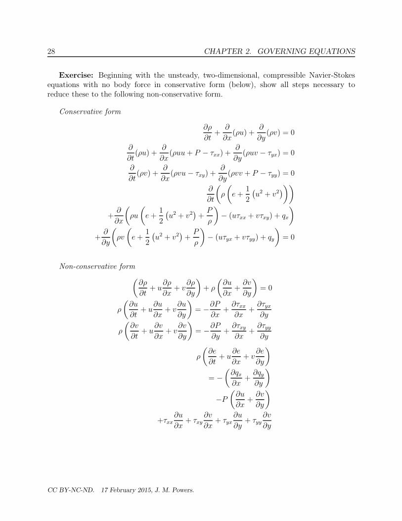
Exercise: Beginning with the unsteady, two-dimensional, compressible Navier-Stokesequations with no body force in conservative form (below), show all steps necessary toreduce these to the following non-conservative form.
Conservative form
∂ρ
∂t+
∂
∂x(ρu) +
∂
∂y(ρv) = 0
∂
∂t(ρu) +
∂
∂x(ρuu+ P − τxx) +
∂
∂y(ρuv − τyx) = 0
∂
∂t(ρv) +
∂
∂x(ρvu− τxy) +
∂
∂y(ρvv + P − τyy) = 0
∂
∂t
(
ρ
(
e+1
2
(
u2 + v2)
))
+∂
∂x
(
ρu
(
e+1
2
(
u2 + v2)
+P
ρ
)
− (uτxx + vτxy) + qx
)
+∂
∂y
(
ρv
(
e+1
2
(
u2 + v2)
+P
ρ
)
− (uτyx + vτyy) + qy
)
= 0
Non-conservative form
(
∂ρ
∂t+ u
∂ρ
∂x+ v
∂ρ
∂y
)
+ ρ
(
∂u
∂x+
∂v
∂y
)
= 0
ρ
(
∂u
∂t+ u
∂u
∂x+ v
∂u
∂y
)
= −∂P
∂x+
∂τxx∂x
+∂τyx∂y
ρ
(
∂v
∂t+ u
∂v
∂x+ v
∂v
∂y
)
= −∂P
∂y+
∂τxy∂x
+∂τyy∂y
ρ
(
∂e
∂t+ u
∂e
∂x+ v
∂e
∂y
)
= −(
∂qx∂x
+∂qy∂y
)
−P
(
∂u
∂x+
∂v
∂y
)
+τxx∂u
∂x+ τxy
∂v
∂x+ τyx
∂u
∂y+ τyy
∂v
∂y
CC BY-NC-ND. 17 February 2015, J. M. Powers.

2.4. CONSTITUTIVE RELATIONS 29
2.4 Constitutive relations
These are determined from experiments and provide sometimes good and sometimes crudemodels for microstructurally based phenomena.
2.4.1 Stress-strain rate relationship for Newtonian fluids
Perform the experiment described in Figure 2.2.
Force = F Velocity = U
h
Figure 2.2: Schematic of experiment to determine stress-strain-rate relationship
The following results are obtained, Figure 2.3:
U
F
U
F h1
h2
h3
h4
h4 > h3 > h2 > h1
A1
A2
A3
A4
A4 > A3 > A2 > A1
Figure 2.3: Force (N) vs. velocity (m/s)
Note for constant plate velocity U
• small gap width h gives large force F
• large cross-sectional area A gives large force F
When scaled by h and A, for a single fluid, the curve collapses to a single curve, Figure2.4:
The viscosity is defined as the ratio of the applied stress τyx = F/A to the strain rate∂u∂y.
CC BY-NC-ND. 17 February 2015, J. M. Powers.

30 CHAPTER 2. GOVERNING EQUATIONS
F/A
U/h
µ
1
Figure 2.4: Stress (N/m2) vs. strain rate (1/s)
µ ≡ τyx∂u∂y
(2.83)
Here the first subscript indicates the face on which the force is acting, here the y face.The second subscript indicates the direction in which the force takes, here the x direction.In general viscous stress is a tensor quantity. In full detail it is as follows:
τ = µ
∂u∂x
+ ∂u∂x
∂u∂y
+ ∂v∂x
∂u∂z
+ ∂w∂x
∂v∂x
+ ∂u∂y
∂v∂y
+ ∂v∂y
∂v∂z
+ ∂w∂y
∂w∂x
+ ∂u∂z
∂w∂y
+ ∂v∂z
∂w∂z
+ ∂w∂z
+λ
∂u∂x
+ ∂v∂y
+ ∂w∂z
0 0
0 ∂u∂x
+ ∂v∂y
+ ∂w∂z
0
0 0 ∂u∂x
+ ∂v∂y
+ ∂w∂z
(2.84)
This is simply an expanded form of that written originally:
τ = µ(
∇v +∇vT)
+ λ (∇ · v) I (2.85)
Here λ is the second coefficient of viscosity. It is irrelevant in incompressible flows andnotoriously difficult to measure in compressible flows. It has been the source of controversyfor over 150 years. Commonly, and only for convenience, people take Stokes’ Assumption:
λ ≡ −2
3µ (2.86)
It can be shown that this results in the mean mechanical stress being equivalent to thethermodynamic pressure.
CC BY-NC-ND. 17 February 2015, J. M. Powers.

2.4. CONSTITUTIVE RELATIONS 31
It can also be shown that the second law is satisfied if
µ ≥ 0 and λ ≥ −2
3µ (2.87)
Example 2.5Couette Flow
Use the linear momentum principle and the constitutive theory to show the velocity profile betweentwo plates is linear. The lower plate at y = 0 is stationary; the upper plate at y = h is moving atvelocity U . Assume v = u(y)i+ 0j+ 0k. Assume there is no imposed pressure gradient or body force.Assume constant viscosity µ. Since u = u(y), v = 0, w = 0, there is no fluid acceleration.
∂u
∂t+ u
∂u
∂x+ v
∂u
∂y+ w
∂u
∂z= 0 + 0 + 0 + 0 = 0 (2.88)
Since no pressure gradient or body force the linear momentum principle is simply
0 =∂τyx∂y
(2.89)
With the Newtonian fluid
0 =∂
∂y
(
µ∂u
∂y
)
(2.90)
With constant µ and u = u(y) we have:
µd2u
dx2= 0 (2.91)
Integrating we findu = Ay +B (2.92)
Use the boundary conditions at y = 0 and y = h to give A and B:
A = 0, B =U
h(2.93)
so
u(y) =U
hy (2.94)
Example 2.6Poiseuille Flow
Consider flow between a slot separated by two plates, the lower at y = 0, the upper at y = h, bothplates stationary. The flow is driven by a pressure difference. At x = 0, P = Po; at x = L, P = P1.The fluid has constant viscosity µ. Assuming the flow is steady, there is no body force, pressure variesonly with x, and that the velocity is only in the x direction and only a function of y; i.e. v = u(y) i,find the velocity profile u(y) parameterized by Po, P1, h, and µ.
CC BY-NC-ND. 17 February 2015, J. M. Powers.

32 CHAPTER 2. GOVERNING EQUATIONS
As before there is no acceleration and the x momentum equation reduces to:
0 = −∂P
∂x+ µ
∂2u
∂y2(2.95)
First let’s find the pressure field; take ∂/∂x:
0 = −∂2P
∂x2+ µ
∂
∂x
(
∂2u
∂y2
)
(2.96)
changing order of differentiation: 0 = −∂2P
∂x2+ µ
∂2
∂y2
(
∂u
∂x
)
(2.97)
0 = −∂2P
∂x2= −d2P
dx2(2.98)
dP
dx= A (2.99)
P = Ax+B (2.100)
apply boundary conditions : P (0) = Po P (L) = P1 (2.101)
P (x) = Po + (P1 − Po)x
L(2.102)
sodP
dx=
(P1 − Po)
L(2.103)
substitute into momentum: 0 = − (P1 − Po)
L+ µ
d2u
dy2(2.104)
d2u
dy2=
(P1 − Po)
µL(2.105)
du
dy=
(P1 − Po)
µLy + C1 (2.106)
u(y) =(P1 − Po)
2µLy2 + C1y + C2 (2.107)
boundary conditions: u(0) = 0 = C2 (2.108)
u(h) = 0 =(P1 − Po)
2µLh2 + C1h+ 0 (2.109)
C1 = − (P1 − Po)
2µLh (2.110)
u(y) =(P1 − Po)
2µL
(
y2 − yh)
(2.111)
wall shear:du
dy=
(P1 − Po)
2µL(2y − h) (2.112)
τwall = µdu
dy
∣
∣
∣
∣
y=0
= −h(P1 − Po)
2L(2.113)
Exercise: Consider flow between a slot separated by two plates, the lower at y = 0, theupper at y = h, with the bottom plate stationary and the upper plate moving at velocity
CC BY-NC-ND. 17 February 2015, J. M. Powers.

2.4. CONSTITUTIVE RELATIONS 33
U . The flow is driven by a pressure difference and the motion of the upper plate. At x = 0,P = Po; at x = L, P = P1. The fluid has constant viscosity µ. Assuming the flow issteady, there is no body force, pressure varies only with x, and that the velocity is only inthe x direction and only a function of y; i.e. v = u(y)i, a) find the velocity profile u(y)parameterized by Po, P1, h, U and µ; b) Find U such that there is no net mass flux betweenthe plates.
2.4.2 Fourier’s law for heat conduction
It is observed in experiment that heat moves from regions of high temperature to low tem-perature Perform the experiment described in Figure 2.5.
T To
L
x
A q
T > To
Figure 2.5: Schematic of experiment to determine thermal conductivity
The following results are obtained, Figure 2.6:
Q
T
Q
T
Q
T
t1
t2
t3
A1
A2
A3
L1
L2
L1
t3 > t2 > t1 A3 > A2 > A1 L3 > L2 > L1
Figure 2.6: Heat transferred (J) vs. temperature (K)
Note for constant temperature of the high temperature reservoir T
• large time of heat transfer t gives large heat transfer Q
• large cross-sectional area A gives large heat transfer Q
• small length L gives large heat transfer Q
When scaled by L, t, and A, for a single fluid, the curve collapses to a single curve, Figure2.7:
CC BY-NC-ND. 17 February 2015, J. M. Powers.

34 CHAPTER 2. GOVERNING EQUATIONS
Q/(A t)
T/L
k
1
Figure 2.7: heat flux vs. temperature gradient
The thermal conductivity is defined as the ratio of the flux of heat transfer qx ∼ Q/(At)to the temperature gradient −∂T
∂x∼ T/L.
k ≡ qx
−∂T∂x
(2.114)
so
qx = −k∂T
∂x(2.115)
or in vector notation:
q = −k∇T (2.116)
Note with this form, the contribution from heat transfer to the entropy production isguaranteed positive if k ≥ 0.
k∇T · ∇T
T 2+
1
Tτ : ∇v ≥ 0 (2.117)
2.4.3 Variable first coefficient of viscosity, µ
In general the first coefficient of viscosity µ is a thermodynamic property which is a strongfunction of temperature and a weak function of pressure.
2.4.3.1 Typical values of µ for air and water
• air at 300 K, 1 atm : 18.46× 10⁻⁶ (Ns)/m2
• air at 400 K, 1 atm : 23.01× 10⁻⁶ (Ns)/m2
• liquid water at 300 K, 1 atm : 855× 10−6 (Ns)/m2
CC BY-NC-ND. 17 February 2015, J. M. Powers.

2.4. CONSTITUTIVE RELATIONS 35
• liquid water at 400 K, 1 atm : 217× 10−6 (Ns)/m2
Note
• viscosity of air an order of magnitude less than water
• ∂µ∂T
> 0 for air, and gases in general
• ∂µ∂T
< 0 for water, and liquids in general
2.4.3.2 Common models for µ
• constant property: µ = µo
• kinetic theory estimate for high temperature gas: µ (T ) = µo
√
TTo
• empirical data
2.4.4 Variable second coefficient of viscosity, λ
Very little data for any material exists for the second coefficient of viscosity. It only plays arole in compressible viscous flows, which are typically very high speed. Some estimates:
• Stokes’ hypothesis: λ = −23µ, may be correct for monatomic gases
• may be inferred from attenuation rates of sound waves
• perhaps may be inferred from shock wave thicknesses
2.4.5 Variable thermal conductivity, k
In general thermal conductivity k is a thermodynamic property which is a strong functionof temperature and a weak function of pressure.
2.4.5.1 Typical values of k for air and water
• air at 300 K, 1 atm : 26.3× 10⁻³ W/(mK)
• air at 400 K, 1 atm : 33.8× 10⁻³ W/(mK)
• liquid water at 300 K, 1 atm : 613× 10−3 W/(mK)
• liquid water at 400 K, 1 atm : 688× 10−3 W/(mK) (the liquid here is supersaturated)
Note
• conductivity of air is one order of magnitude less than water
• ∂k∂T
> 0 for air, and gases in general
• ∂k∂T
> 0 for water in this range, generalization difficult
CC BY-NC-ND. 17 February 2015, J. M. Powers.

36 CHAPTER 2. GOVERNING EQUATIONS
2.4.5.2 Common models for k
• constant property: k = ko
• kinetic theory estimate for high temperature gas: k (T ) = ko
√
TTo
• empirical data
Exercise: Consider one-dimensional steady heat conduction in a fluid at rest. At x =0 m at constant heat flux is applied qx = 10 W/m2. At x = 1 m, the temperature is heldconstant at 300 K. Find T (y), T (0) and qx(1) for
• liquid water with k = 613× 10−3 W/(mK)
• air with k = 26.3× 10⁻³ W/(mK)
• air with k =(
26.3× 10⁻³√
T300
)
W/(mK)
2.4.6 Thermal equation of state
2.4.6.1 Description
• determined in static experiments
• gives P as a function of ρ and T
2.4.6.2 Typical models
• ideal gas: P = ρRT
• first virial: P = ρRT (1 + b1ρ)
• general virial: P = ρRT (1 + b1ρ+ b2ρ2 + ...)
• van der Waals: P = RT (1/ρ− b)−1 − aρ2
2.4.7 Caloric equation of state
2.4.7.1 Description
• determined in experiments
• gives e as function of ρ and T in general
• arbitrary constant appears
• must also be thermodynamically consistent via relation to be discussed later:
CC BY-NC-ND. 17 February 2015, J. M. Powers.

2.5. SPECIAL CASES OF GOVERNING EQUATIONS 37
de = cv (T ) dT −(
1
ρ2
)
(
T∂P
∂T
∣
∣
∣
∣
ρ
− P
)
dρ (2.118)
With knowledge of cv(T ) and P (ρ, T ), the above can be integrated to find e.
2.4.7.2 Typical models
• consistent with ideal gas:
– constant specific heat: e(T ) = cvo (T − To) + eo
– temperature dependent specific heat: e(T ) =∫ T
Tocv(T )dT + eo
• consistent with first virial: e(T ) =∫ T
Tocv(T )dT + eo
• consistent with van der Waals: e(ρ, T ) =∫ T
Tocv(T )dT +−a (ρ− ρo) + eo
2.5 Special cases of governing equations
The governing equations are often expressed in more simple forms in common limits. Someare listed here.
2.5.1 One-dimensional equations
Most of the mystery of vector notation is removed in the one-dimensional limit where v =w = 0, ∂
∂y= ∂
∂z= 0; additionally we adopt Stokes assumption λ = −(2/3)µ:
(
∂ρ
∂t+ u
∂ρ
∂x
)
+ ρ∂u
∂x= 0 (2.119)
ρ
(
∂u
∂t+ u
∂u
∂x
)
= −∂P
∂x+
∂
∂x
(
4
3µ∂u
∂x
)
+ ρgx (2.120)
ρ
(
∂e
∂t+ u
∂e
∂x
)
=∂
∂x
(
k∂T
∂x
)
− P∂u
∂x+
4
3µ
(
∂u
∂x
)2
(2.121)
µ = µ (ρ, T ) (2.122)
k = k (ρ, T ) (2.123)
P = P (ρ, T ) (2.124)
e = e (ρ, T ) (2.125)
note: 7 equations, 7 unknowns: (ρ, u, P, e, T, µ, k)
CC BY-NC-ND. 17 February 2015, J. M. Powers.
38 CHAPTER 2. GOVERNING EQUATIONS
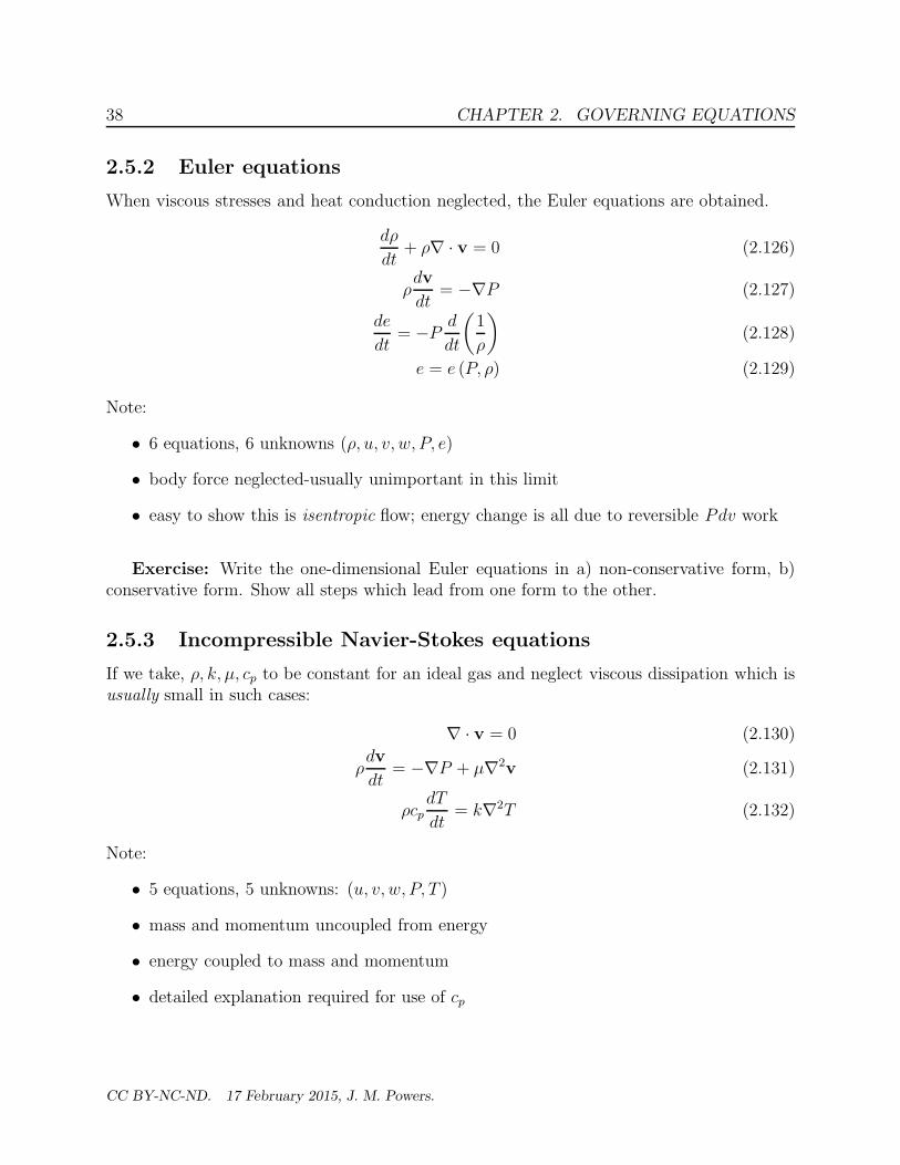
2.5.2 Euler equations
When viscous stresses and heat conduction neglected, the Euler equations are obtained.
dρ
dt+ ρ∇ · v = 0 (2.126)
ρdv
dt= −∇P (2.127)
de
dt= −P
d
dt
(
1
ρ
)
(2.128)
e = e (P, ρ) (2.129)
Note:
• 6 equations, 6 unknowns (ρ, u, v, w, P, e)
• body force neglected-usually unimportant in this limit
• easy to show this is isentropic flow; energy change is all due to reversible Pdv work
Exercise: Write the one-dimensional Euler equations in a) non-conservative form, b)conservative form. Show all steps which lead from one form to the other.
2.5.3 Incompressible Navier-Stokes equations
If we take, ρ, k, µ, cp to be constant for an ideal gas and neglect viscous dissipation which isusually small in such cases:
∇ · v = 0 (2.130)
ρdv
dt= −∇P + µ∇2v (2.131)
ρcpdT
dt= k∇2T (2.132)
Note:
• 5 equations, 5 unknowns: (u, v, w, P, T )
• mass and momentum uncoupled from energy
• energy coupled to mass and momentum
• detailed explanation required for use of cp
CC BY-NC-ND. 17 February 2015, J. M. Powers.

Chapter 3
Thermodynamics review
Suggested Reading:
Liepmann and Roshko, Chapter 1: pp. 1-24, 34-38
Shapiro, Chapter 2: pp. 23-44
Anderson, Chapter 1: pp. 12-25
As we have seen from the previous chapter, the subject of thermodynamics is a subset ofthe topic of viscous compressible flows. It is almost always necessary to consider the thermo-dynamics as part of a larger coupled system in design. This is in contrast to incompressibleaerodynamics which can determine forces independent of the thermodynamics.
3.1 Preliminary mathematical concepts
Ifz = z(x, y) (3.1)
then
dz =∂z
∂x
∣
∣
∣
∣
y
dx+∂z
∂y
∣
∣
∣
∣
x
dy (3.2)
which is of the formdz = Mdx+Ndy (3.3)
Now
∂M
∂y=
∂
∂y
∂z
∂x(3.4)
∂N
∂x=
∂
∂x
∂z
∂y(3.5)
thus∂M
∂y=
∂N
∂x(3.6)
so the implication is that if we are given dz,M,N , we can form z only if the above holds.
39

40 CHAPTER 3. THERMODYNAMICS REVIEW
3.2 Summary of thermodynamic concepts
• property: characterizes the thermodynamics state of the system
– extensive: proportional to system’s mass, upper case variable E, S,H
– intensive: independent of system’s mass, lower case variable e, s, h, (exceptionsT, P )
• equations of state: relate properties
• Any intensive thermodynamic property can be expressed as a function of at most twoother intensive thermodynamic properties (for simple systems)
– P = ρRT : thermal equation of state for ideal gas
– c =√
γ Pρ: sound speed for calorically perfect ideal gas
• first law: dE = δQ− δW
• second law: dS ≥ δQ/T
• process: moving from one state to another, in general with accompanying heat transferand work
• cycle: process which returns to initial state
• reversible work: w12 =∫ 2
1Pdv
• reversible heat transfer: q12 =∫ 2
1Tds
Figure 3.1 gives a sketch of an isothermal thermodynamic process going from state 1 tostate 2. The figure shows a variety of planes, P − v, T − s, P − T , and v − T . For idealgases, 1) isotherms are hyperbolas in the P −v plane: P = (RT )/v, 2) isochores are straightlines in the P − T plane: P = (R/v)T , with large v giving a small slope, and 3) isobarsare straight lines in the v − T plane: v = (RT )/P , with large P giving a small slope. Thearea under the curve in the P − v plane gives the work. The area under the curve in theT − s plane gives the heat transfer. The energy change is given by the difference in the heattransfer and the work. The isochores in the T − s plane are non-trivial. For a caloricallyperfect ideal gas, they are given by exponential curves.
Figure 3.2 gives a sketch of a thermodynamic cycle. Here we only sketch the P − v andT − s planes, though others could be included. Since it is a cyclic process, there is no netenergy change for the cycle and the cyclic work equals the cyclic heat transfer. The enclosedarea in the P − v plane, i.e. the net work, equals the enclosed area in the T − s plane, i.e.the net heat transfer. The sketch has the cycle working in the direction which correspondsto an engine. A reversal of the direction would correspond to a refrigerator.
CC BY-NC-ND. 17 February 2015, J. M. Powers.

3.2. SUMMARY OF THERMODYNAMIC CONCEPTS 41
v
P
T = T1
v2v1
12 122 1∫w = P dv 12 1
2
s
T
∫q = T ds 12 1
2e - e = q - w
v2
v1
s2s1
T
P
T
vv1
v2
2T = T
1
v1
v2
2
1
2
P
P
1P
2P
T = T1 2
2T = T
1
1P
2P
Figure 3.1: Sketch of isothermal thermodynamic process
Example 3.1Consider the following isobaric process for air, modelled as a calorically perfect ideal gas, from state
1 to state 2. P1 = 100 kPa, T1 = 300 K, T2 = 400 K.
Since the process is isobaric P = 100 kPa describes a straight line in P − v and P − T planes andP2 = P1 = 100 kPa. Since ideal gas, v − T plane:
v =
(
R
P
)
T straight lines! (3.7)
v1 = RT1/P1 =(287 J/kg/K) (300 K)
100, 000 Pa= 0.861 m3/kg (3.8)
v2 = RT2/P2 =(287 J/kg/K) (400 K)
100, 000 Pa= 1.148 m3/kg (3.9)
Since calorically perfect:
de = cvdT (3.10)∫ e1
e2
de = cv
∫ T1
T2
dT (3.11)
e2 − e1 = cv(T2 − T1) (3.12)
= (716.5 J/kg/K) (400 K − 300 K) (3.13)
= 71, 650 J/kg (3.14)
CC BY-NC-ND. 17 February 2015, J. M. Powers.

42 CHAPTER 3. THERMODYNAMICS REVIEW
v
P
s
T
q = wcycle cycle
Figure 3.2: Sketch of thermodynamic cycle
also
Tds = de+ Pdv (3.15)
Tds = cvdT + Pdv (3.16)
from ideal gas : v =RT
P: dv =
R
PdT − RT
P 2dP (3.17)
Tds = cvdT +RdT − RT
PdP (3.18)
ds = (cv +R)dT
T−R
dP
P(3.19)
ds = (cv + cp − cv)dT
T−R
dP
P(3.20)
ds = cpdT
T−R
dP
P(3.21)
∫ s2
s1
ds = cp
∫ T2
T1
dT
T−R
∫ P2
P1
dP
P(3.22)
s2 − s1 = cp ln
(
T2
T1
)
−R ln
(
P2
P1
)
(3.23)
s− so = cp ln
(
T
To
)
−R ln
(
P
Po
)
(3.24)
since P = constant: (3.25)
s2 − s1 = cp ln
(
T2
T1
)
(3.26)
= (1003.5 J/kg/K) ln
(
400 K
300 K
)
(3.27)
= 288.7 J/kg/K (3.28)
w12 =
∫ v2
v1
Pdv = P
∫ v2
v1
dv (3.29)
= P (v2 − v1) (3.30)
CC BY-NC-ND. 17 February 2015, J. M. Powers.

3.2. SUMMARY OF THERMODYNAMIC CONCEPTS 43
= (100, 000 Pa)(1.148 m3/kg − 0.861 m3/kg) (3.31)
= 29, 600 J/kg (3.32)
Now
de = δq − δw (3.33)
δq = de+ δw (3.34)
q12 = (e2 − e1) + w12 (3.35)
q12 = 71, 650 J/kg + 29, 600 J/kg (3.36)
q12 = 101, 250 J/kg (3.37)
Now in this process the gas is heated from 300 K to 400 K. We would expect at a minimum that thesurroundings were at 400 K. Let’s check for second law satisfaction.
s2 − s1 ≥ q12Tsurr
? (3.38)
288.7 J/kg/K ≥ 101, 250 J/kg
400 K? (3.39)
288.7 J/kg/K ≥ 253.1 J/kg/K yes (3.40)
v
P
T = 300 K1
T2
v2v1
P = P = 100 kPa 1 2
12 122 1∫w = P dv 12 1
2
s
T
∫q = T ds 12 1
2e - e = q - w
v2
v1
s2s1
T
T1
2
T
P
T
vv1
v2
T2
T1
P = P = 100 kPa 1 2
P = P = 100 kPa 1 2
T1 T
2
v1
v2
Figure 3.3: Sketch for isobaric example problem
CC BY-NC-ND. 17 February 2015, J. M. Powers.

44 CHAPTER 3. THERMODYNAMICS REVIEW
3.3 Maxwell relations and secondary properties
Recall
de = Tds− Pd
(
1
ρ
)
(3.41)
Since v ≡ 1/ρ we get
de = Tds− Pdv (3.42)
Now we assume e = e(s, v),
de =∂e
∂s
∣
∣
∣
∣
v
ds+∂e
∂v
∣
∣
∣
∣
s
dv (3.43)
Thus
T =∂e
∂s
∣
∣
∣
∣
v
P = − ∂e
∂v
∣
∣
∣
∣
s
(3.44)
and
∂T
∂v
∣
∣
∣
∣
s
=∂2e
∂v∂s
∂P
∂s
∣
∣
∣
∣
v
= − ∂2e
∂s∂v(3.45)
Thus we get a Maxwell relation:
∂T
∂v
∣
∣
∣
∣
s
= − ∂P
∂s
∣
∣
∣
∣
v
(3.46)
Define the following properties:
• enthalpy: h ≡ e + pv
• Helmholtz free energy: a ≡ e− Ts
• Gibbs free energy: g ≡ h− Ts
Now with these definitions it is easy to form differential relations using the Gibbs relationas a root.
h = e+ Pv (3.47)
dh = de+ Pdv + vdP (3.48)
de = dh− Pdv − vdP (3.49)
substitute into Gibbs: de = Tds− Pdv (3.50)
dh− Pdv − vdP = Tds− Pdv (3.51)
dh = Tds+ vdP (3.52)
CC BY-NC-ND. 17 February 2015, J. M. Powers.

3.3. MAXWELL RELATIONS AND SECONDARY PROPERTIES 45
So s and P are natural variables for h. Through a very similar process we get the followingrelationships:
∂h
∂s
∣
∣
∣
∣
P
= T∂h
∂P
∣
∣
∣
∣
s
= v (3.53)
∂a
∂v
∣
∣
∣
∣
T
= −P∂a
∂T
∣
∣
∣
∣
v
= −s (3.54)
∂g
∂P
∣
∣
∣
∣
T
= v∂g
∂T
∣
∣
∣
∣
P
= −s (3.55)
∂T
∂P
∣
∣
∣
∣
s
=∂v
∂s
∣
∣
∣
∣
P
∂P
∂T
∣
∣
∣
∣
v
=∂s
∂v
∣
∣
∣
∣
T
∂v
∂T
∣
∣
∣
∣
P
= − ∂s
∂P
∣
∣
∣
∣
T
(3.56)
The following thermodynamic properties are also useful and have formal definitions:
• specific heat at constant volume: cv ≡ ∂e∂T
∣
∣
v
• specific heat at constant pressure: cp ≡ ∂h∂T
∣
∣
P
• ratio of specific heats: γ ≡ cp/cv
• sound speed: c ≡√
∂P∂ρ
∣
∣
∣
s
• adiabatic compressibility: βs ≡ − 1v
∂v∂P
∣
∣
s
• adiabatic bulk modulus: Bs ≡ −v ∂P∂v
∣
∣
s
Generic problem: given P = P (T, v), find other properties
3.3.1 Internal energy from thermal equation of state
Find the internal energy e(T, v) for a general material.
e = e(T, v) (3.57)
de =∂e
∂T
∣
∣
∣
∣
v
dT +∂e
∂v
∣
∣
∣
∣
T
dv (3.58)
de = cvdT +∂e
∂v
∣
∣
∣
∣
T
dv (3.59)
Now from Gibbs,
de = Tds− Pdv (3.60)
de
dv= T
ds
dv− P (3.61)
∂e
∂v
∣
∣
∣
∣
T
= T∂s
∂v
∣
∣
∣
∣
T
− P (3.62)
CC BY-NC-ND. 17 February 2015, J. M. Powers.

46 CHAPTER 3. THERMODYNAMICS REVIEW
Substitute from Maxwell relation,
∂e
∂v
∣
∣
∣
∣
T
= T∂P
∂T
∣
∣
∣
∣
v
− P (3.63)
so
de = cvdT +
(
T∂P
∂T
∣
∣
∣
∣
v
− P
)
dv (3.64)
∫ e
eo
de =
∫ T
To
cv(T )dT +
∫ v
vo
(
T∂P
∂T
∣
∣
∣
∣
∣
v
− P
)
dv (3.65)
e(T, v) = eo +
∫ T
To
cv(T )dT +
∫ v
vo
(
T∂P
∂T
∣
∣
∣
∣
∣
v
− P
)
dv (3.66)
Example 3.2Ideal gas
Find a general expression for e(T, v) if
P (T, v) =RT
v(3.67)
Proceed as follows:
∂P
∂T
∣
∣
∣
∣
v
= R/v (3.68)
T∂P
∂T
∣
∣
∣
∣
v
− P =RT
v− P (3.69)
=RT
v− RT
v= 0 (3.70)
Thus e is
e(T ) = eo +
∫ T
To
cv(T )dT (3.71)
We also find
h = e+ Pv = eo +
∫ T
To
cv(T )dT + Pv (3.72)
h(T, v) = eo +
∫ T
To
cv(T )dT +RT (3.73)
cp(T, v) =≡ ∂h
∂T
∣
∣
∣
∣
P
= cv(T ) +R = cp(T ) (3.74)
R = cp(T )− cv(T ) (3.75)
Iff cv is a constant then
e(T ) = eo + cv(T − To) (3.76)
h(T ) = (eo + Povo) + cp(T − To) (3.77)
R = cp − cv (3.78)
CC BY-NC-ND. 17 February 2015, J. M. Powers.

3.3. MAXWELL RELATIONS AND SECONDARY PROPERTIES 47
Example 3.3van der Waals gas
Find a general expression for e(T, v) if
P (T, v) =RT
v − b− a
v2(3.79)
Proceed as before:
∂P
∂T
∣
∣
∣
∣
v
=R
v − b(3.80)
T∂P
∂T
∣
∣
∣
∣
v
− P =RT
v − b− P (3.81)
=RT
v − b−(
RT
v − b− a
v2
)
=a
v2(3.82)
Thus e is
e(T, v) = eo +
∫ T
To
cv(T )dT +
∫ v
vo
a
v2dv (3.83)
= eo +
∫ T
To
cv(T )dT + a
(
1
vo− 1
v
)
(3.84)
We also find
h = e+ Pv = eo +
∫ T
To
cv(T )dT + a
(
1
vo− 1
v
)
+ Pv (3.85)
h(T, v) = eo +
∫ T
To
cv(T )dT + a
(
1
vo− 1
v
)
+RTv
v − b− a
v(3.86)
(3.87)
3.3.2 Sound speed from thermal equation of state
Find the sound speed c(T, v) for a general material.
c =
√
∂P
∂ρ
∣
∣
∣
∣
s
(3.88)
c2 =∂P
∂ρ
∣
∣
∣
∣
s
(3.89)
CC BY-NC-ND. 17 February 2015, J. M. Powers.

48 CHAPTER 3. THERMODYNAMICS REVIEW
Use Gibbs relation
Tds = de+ Pdv (3.90)
(3.91)
Substitute earlier relation for de
Tds =
[
cvdT +
(
T∂P
∂T
∣
∣
∣
∣
v
− P
)
dv
]
+ Pdv (3.92)
Tds = cvdT + T∂P
∂T
∣
∣
∣
∣
v
dv (3.93)
Tds = cvdT − T
ρ2∂P
∂T
∣
∣
∣
∣
ρ
dρ (3.94)
Since P = P (T, v), P = P (T, ρ)
dP =∂P
∂T
∣
∣
∣
∣
ρ
dT +∂P
∂ρ
∣
∣
∣
∣
T
dρ (3.95)
dT =dP − ∂P
∂ρ
∣
∣
∣
Tdρ
∂P∂T
∣
∣
ρ
(3.96)
Thus substituting for dT
Tds = cv
dP − ∂P∂ρ
∣
∣
∣
Tdρ
∂P∂T
∣
∣
ρ
− T
ρ2∂P
∂T
∣
∣
∣
∣
ρ
dρ (3.97)
so grouping terms in dP and dρ we get
Tds =
(
cv∂P∂T
∣
∣
ρ
)
dP −
cv
∂P∂ρ
∣
∣
∣
T∂P∂T
∣
∣
ρ
+T
ρ2∂P
∂T
∣
∣
∣
∣
ρ
dρ (3.98)
SO if ds ≡ 0 we obtain
∂P
∂ρ
∣
∣
∣
∣
s
=1
cv
∂P
∂T
∣
∣
∣
∣
ρ
cv
∂P∂ρ
∣
∣
∣
T∂P∂T
∣
∣
ρ
+T
ρ2∂P
∂T
∣
∣
∣
∣
ρ
(3.99)
=∂P
∂ρ
∣
∣
∣
∣
T
+T
cvρ2
(
∂P
∂T
∣
∣
∣
∣
ρ
)2
(3.100)
So
c(T, ρ) =
√
√
√
√
∂P
∂ρ
∣
∣
∣
∣
T
+T
cvρ2
(
∂P
∂T
∣
∣
∣
∣
ρ
)2
(3.101)
CC BY-NC-ND. 17 February 2015, J. M. Powers.

3.3. MAXWELL RELATIONS AND SECONDARY PROPERTIES 49
Exercises: Liepmann and Roshko, 1.3 and 1.4, p. 383.
Example 3.4Ideal gas
Find the sound speed if
P (T, ρ) = ρRT (3.102)
The necessary partials are
∂P
∂ρ
∣
∣
∣
∣
T
= RT∂P
∂T
∣
∣
∣
∣
ρ
= ρR (3.103)
so
c(T, ρ) =
√
RT +T
cvρ2(ρR)
2(3.104)
=
√
RT +R2T
cv(3.105)
=
√
RT
(
1 +R
cv
)
(3.106)
=
√
RT
(
1 +cP − cv
cv
)
(3.107)
=
√
RT
(
cv + cP − cvcv
)
(3.108)
=√
γRT (3.109)
Sound speed depends on temperature alone for the calorically perfect ideal gas.
Example 3.5Virial gas
Find the sound speed if
P (T, ρ) = ρRT (1 + b1ρ) (3.110)
The necessary partials are
∂P
∂ρ
∣
∣
∣
∣
T
= RT + 2b1ρRT∂P
∂T
∣
∣
∣
∣
ρ
= ρR (1 + b1ρ) (3.111)
CC BY-NC-ND. 17 February 2015, J. M. Powers.

50 CHAPTER 3. THERMODYNAMICS REVIEW
so
c(T, ρ) =
√
RT + 2b1ρRT +T
cvρ2(ρR (1 + b1ρ))
2 (3.112)
=
√
RT
(
1 + 2b1ρ+R
cv(1 + b1ρ)2
)
(3.113)
Sound speed depends on both temperature and density.
Example 3.6Thermodynamic process with a van der Waals Gas
A van der Waals gas with
R = 200 J/kg/K (3.114)
a = 150 Pa m6/kg2 (3.115)
b = 0.001 m3/kg (3.116)
cv = [350 + 0.2(T − 300K)] J/kg/K (3.117)
begins at T1 = 300 K, P1 = 1×10⁵ Pa. It is isothermally compressed to state 2 where P2 = 1×10⁶ Pa.It is then isochorically heated to state 3 where T3 = 1, 000 K. Find w13, q13, and s3 − s1. Assume thesurroundings are at 1, 000 K. Recall
P =RT
v − b− a
v2(3.118)
so at state 1
100, 000 =200× 300
v1 − 0.001− 150
v21(3.119)
or expanding
−0.15 + 150v − 60, 100v2 + 100, 000v3 = 0 (3.120)
Cubic equation–three solutions:
v1 = 0.598 m3/kg (3.121)
v1 = 0.00125− 0.0097i m3/kg not physical (3.122)
v1 = 0.00125 + 0.0097i m3/kg not physical (3.123)
Now at state 2 we know P2 and T2 so we can determine v2
1, 000, 000 =200× 300
v2 − 0.001− 150
v22(3.124)
The physical solution is v2 = 0.0585 m3/kg. Now at state 3 we know v3 = v2 and T3. Determine P3:
P3 =200× 1, 000
0.0585− 0.001− 150
0.05852= 3, 478, 261− 43, 831 = 3, 434, 430 Pa (3.125)
CC BY-NC-ND. 17 February 2015, J. M. Powers.

3.3. MAXWELL RELATIONS AND SECONDARY PROPERTIES 51
Now w13 = w12 + w23 =∫ 2
1Pdv +
∫ 3
2Pdv =
∫ 2
1Pdv since 2− 3 is at constant volume. So
w13 =
∫ v2
v1
(
RT
v − b− a
v2
)
dv (3.126)
= RT1
∫ v2
v1
dv
v − b− a
∫ v2
v1
dv
v2(3.127)
= RT1 ln
(
v2 − b
v1 − b
)
+ a
(
1
v2− 1
v1
)
(3.128)
= 200× 300 ln
(
0.0585− 0.001
0.598− 0.001
)
+ 150
(
1
0.0585− 1
0.598
)
(3.129)
= −140, 408+ 2, 313 (3.130)
= −138, 095 J/kg = −138 kJ/kg (3.131)
The gas is compressed, so the work is negative. Since e is a state property:
e3 − e1 =
∫ T3
T1
cv(T )dT + a
(
1
v1− 1
v3
)
(3.132)
Now
cv = 350 + 0.2(T − 300) = 290 +1
5T (3.133)
so
e3 − e1 =
∫ T3
T1
(
290 +1
5T
)
dT + a
(
1
v1− 1
v3
)
(3.134)
= 290 (T3 − T1) +1
10
(
T 23 − T 2
1
)
+ a
(
1
v1− 1
v3
)
(3.135)
290 (1, 000− 300) +1
10
(
1, 0002 − 3002)
+ 150
(
1
0.598− 1
0.0585
)
(3.136)
= 203, 000+ 91, 000− 2, 313 (3.137)
= 291, 687 J/kg = 292 kJ/kg (3.138)
Now from the first law
e3 − e1 = q13 − w13 (3.139)
q13 = e3 − e1 + w13 (3.140)
q13 = 292− 138 (3.141)
q13 = 154 kJ/kg (3.142)
The heat transfer is positive as heat was added to the system.
Now find the entropy change. Manipulate the Gibbs equation:
Tds = de+ Pdv (3.143)
ds =1
Tde+
P
Tdv (3.144)
ds =1
T
(
cv(T )dT +a
v2dv)
+P
Tdv (3.145)
CC BY-NC-ND. 17 February 2015, J. M. Powers.

52 CHAPTER 3. THERMODYNAMICS REVIEW
ds =1
T
(
cv(T )dT +a
v2dv)
+1
T
(
RT
v − b− a
v2
)
dv (3.146)
ds =cv(T )
TdT +
R
v − bdv (3.147)
s3 − s1 =
∫ T3
T1
cv(T )
TdT +R ln
v3 − b
v1 − b(3.148)
=
∫ 1,000
300
(
290
T+
1
5
)
dT +R lnv3 − b
v1 − b(3.149)
= 290 ln1, 000
300+
1
5(1, 000− 300) + 200 ln
0.0585− 0.001
0.598− 0.001(3.150)
= 349 + 140− 468 (3.151)
= 21J
kg K= 0.021
kJ
kg K(3.152)
Is the second law satisfied for each portion of the process?
First look at 1 → 2
e2 − e1 = q12 − w12 (3.153)
q12 = e2 − e1 + w12 (3.154)
q12 =
(
∫ T2
T1
cv(T )dT + a
(
1
v1− 1
v2
)
)
+
(
RT1 ln
(
v2 − b
v1 − b
)
+ a
(
1
v2− 1
v1
))
(3.155)
(3.156)
Since T1 = T2 and canceling the terms in a we get
q12 = RT1 ln
(
v2 − b
v1 − b
)
= 200× 300 ln
(
0.0585− 0.001
0.598− 0.001
)
= −140, 408J
kg(3.157)
Since isothermal
s2 − s1 = R ln
(
v2 − b
v1 − b
)
(3.158)
= 200 ln
(
0.0585− 0.001
0.598− 0.001
)
(3.159)
= −468.0J
kg K(3.160)
Entropy drops because heat was transferred out of the system.
Check the second law. Note that in this portion of the process in which the heat is transferred outof the system, that the surroundings must have Tsurr ≤ 300 K. For this portion of the process let ustake Tsurr = 300 K.
s2 − s1 ≥ q12T
? (3.161)
−468.0J
kg K≥
−140, 408 Jkg
300 K(3.162)
−468.0J
kg K≥ −468.0
J
kg Kok (3.163)
CC BY-NC-ND. 17 February 2015, J. M. Powers.

3.4. CANONICAL EQUATIONS OF STATE 53
Next look at 2 → 3
q23 = e3 − e2 + w23 (3.164)
q23 =
(
∫ T3
T2
cv(T )dT + a
(
1
v2− 1
v3
)
)
+
(∫ v3
v2
Pdv
)
(3.165)
since isochoric q23 =
∫ T3
T2
cv(T )dT (3.166)
=
∫ 1000
300
(
290 +T
5
)
dT = 294, 000J
K(3.167)
Now look at the entropy change for the isochoric process:
s3 − s2 =
∫ T3
T2
cv(T )
TdT (3.168)
=
∫ T3
T2
(
290
T+
1
5
)
dT (3.169)
= 290 ln1, 000
300+
1
5(1, 000− 300) = 489
J
kg K(3.170)
Entropy rises because heat transferred into system.
In order to transfer heat into the system we must have a different thermal reservoir. This one musthave Tsurr ≥ 1000 K. Assume here that the heat transfer was from a reservoir held at 1, 000 K toassess the influence of the second law.
s3 − s2 ≥ q23T
? (3.171)
489J
kg K≥
294, 000 Jkg
1, 000 K(3.172)
489J
kg K≥ 294
J
kg Kok (3.173)
3.4 Canonical equations of state
If we have a single equation of state in a special canonical form, we can form both thermaland caloric equations. Since
de = Tds− Pdv (3.174)
dh = Tds+ vdP (3.175)
it is suggested that the form
e = e(s, v) (3.176)
h = h(s, P ) (3.177)
CC BY-NC-ND. 17 February 2015, J. M. Powers.

54 CHAPTER 3. THERMODYNAMICS REVIEW
is useful.
Example 3.7Canonical Form
If
h(s, P ) = KcpPR/cp exp
(
s
cp
)
+ (ho − cpTo) (3.178)
derive both thermal and caloric state equations P (v, T ) and e(v, T ).
Now for our material
∂h
∂s
∣
∣
∣
∣
P
= KPR/cp exp
(
s
cp
)
(3.179)
∂h
∂P
∣
∣
∣
∣
s
= KRPR/cp−1 exp
(
s
cp
)
(3.180)
Now since
∂h
∂s
∣
∣
∣
∣
P
= T (3.181)
∂h
∂P
∣
∣
∣
∣
s
= v (3.182)
we have
T = KPR/cp exp
(
s
cp
)
(3.183)
v = KRPR/cp−1 exp
(
s
cp
)
(3.184)
Dividing one by the other gives
T
v=
P
R(3.185)
P =RT
v(3.186)
Substituting our expression for T into our canonical equation for h we also get
h = cpT + (ho − cpTo) (3.187)
h = cp(T − To) + ho (3.188)
which is useful in itself. Substituting in for T and To
h = cp
(
Pv
R− Povo
R
)
+ ho (3.189)
Using h ≡ e+ Pv we get
e+ Pv = cp
(
Pv
R− Povo
R
)
+ eo + Povo (3.190)
CC BY-NC-ND. 17 February 2015, J. M. Powers.
3.5. ISENTROPIC RELATIONS 55
so
e =(cpR
− 1)
Pv −(cpR
− 1)
Povo + eo (3.191)
e =(cpR
− 1)
(Pv − Povo) + eo (3.192)
e =(cpR
− 1)
(RT −RTo) + eo (3.193)
e = (cp −R) (T − To) + eo (3.194)
e = [cp − (cp − cv)] (T − To) + eo (3.195)
e = cv (T − To) + eo (3.196)
So one canonical equation gives us all the information we need! Oftentimes, it is difficult to do asingle experiment to get the canonical form.
Exercise: For a calorically perfect ideal gas, write the Helmholtz free energy and Gibbsfree energy in canonical form, i.e. what is a(T, v), g(P, T )?
3.5 Isentropic relations
Of particular importance in thermodynamics in general and compressible flow in particularare relations that describe an isentropic process, s = constant. Recall the second law.
ds ≥ δq
T(3.197)
If the process is reversible,
ds =δq
T(3.198)
If the process is adiabatic
δq ≡ 0 so ds = 0 (3.199)
So an isentropic process is both adiabatic and reversible. We know from the first law writtenin terms of entropy that this implies that
q ≡ 0 (3.200)
τ ≡ 0 (3.201)
In this case the Gibbs relation and the first law reduce to the same expression:
de = −Pdv (3.202)
That is the energy change is all due to reversible pressure volume work.
We would like to develop an expression between two variables for an isentropic process.
With knowledge of P (T, v)
CC BY-NC-ND. 17 February 2015, J. M. Powers.

56 CHAPTER 3. THERMODYNAMICS REVIEW
• form e(T, v)
• eliminate T to form e(P, v)
• take derivative and substitute into Gibbs/First Law
∂e
∂P
∣
∣
∣
∣
v
dP +∂e
∂v
∣
∣
∣
∣
P
dv = −Pdv (3.203)
∂e
∂P
∣
∣
∣
∣
v
dP +
(
∂e
∂v
∣
∣
∣
∣
P
+ P
)
dv = 0 (3.204)
Integration of this equation gives a relationship between P and v.
Example 3.8Calorically Perfect Ideal Gas
Find the relationship for a calorically perfect ideal gas which undergoes an isentropic process.
Ideal Gas:Pv = RT (3.205)
Calorically Perfect:e = cvT + eo (3.206)
Thus
e = cvPv
R+ eo =
cvcP − cv
Pv + eo =1
γ − 1Pv + eo (3.207)
Thus the necessary derivatives are
∂e
∂P
∣
∣
∣
∣
v
=1
γ − 1v (3.208)
∂e
∂v
∣
∣
∣
∣
P
=1
γ − 1P (3.209)
so substituting into our developed relationship gives
1
γ − 1vdP +
(
1
γ − 1P + P
)
dv = 0 (3.210)
vdP + γPdv = 0 (3.211)
dP
P= −γ
dv
v(3.212)
lnP
Po= −γ ln
v
vo(3.213)
lnP
Po= ln
(vov
)γ
(3.214)
P
Po=(vov
)γ
(3.215)
Pvγ = Povγo = constant (3.216)
CC BY-NC-ND. 17 February 2015, J. M. Powers.

3.5. ISENTROPIC RELATIONS 57
also using the thermal state equation
P
Po=
RTv
RTo
vo
=T
To
vov
=(vov
)γ
(3.217)
T
To=(vov
)γ−1
=
(
P
Po
)γ−1
γ
(3.218)
Find the work in a process from v1 to v2
w12 =
∫ 1
2
Pdv (3.219)
= Povγo
∫ v2
v1
dv
vγ(3.220)
= Povγo
[
v1−γ
1− γ
]v2
v1
(3.221)
=Pov
γo
1− γ
(
v1−γ2 − v1−γ
1
)
(3.222)
=P2v2 − P1v1
1− γ(3.223)
Also
de = δq − δw = 0− δw so (3.224)
e2 − e1 =P2v2 − P1v1
γ − 1(3.225)
Figure 3.4 gives a sketch for the calorically perfect ideal gas undergoing an isentropicexpansion in various planes.
Example 3.9Virial Gas
Find the relationship between P and v for a virial gas with constant cv which undergoes an isentropicprocess.
Virial Gas:
P =RT
v − b(3.226)
This is van der Waals with a = 0 and cv constant so:
e = cvT + eo (3.227)
Thus
e = cvP (v − b)
R+ eo (3.228)
CC BY-NC-ND. 17 February 2015, J. M. Powers.

58 CHAPTER 3. THERMODYNAMICS REVIEW
v
P
T 2
T1
v2
v1
12 122 1∫w = P dv 12 1
2
s
T
∫q = T ds 12 1
2e - e = q - w
v2
v1
s2s =1
T
T
1
2
T
P
T
v
v1
v2
T1
T2
T1
T2
v1
v2
P
P
1
2
P2
P1
P
P
1
2
Figure 3.4: Sketch of isentropic expansion process
Thus the necessary derivatives are
∂e
∂P
∣
∣
∣
∣
v
=cvR
(v − b) (3.229)
∂e
∂v
∣
∣
∣
∣
P
=cvRP (3.230)
so substituting into our developed relationship gives
cvR
(v − b) dP +(cvRP + P
)
dv = 0 (3.231)
(v − b)dP +
(
1 +R
cv
)
Pdv = 0 (3.232)
with γ ≡ 1 +R
cv(3.233)
dP
dv+
γ
v − bP = 0 (3.234)
(
exp
∫
γ
v − bdv
)
dP
dv+
(
exp
∫
γ
v − bdv
)
γ
v − bP = 0 (3.235)
(
exp(
ln (v − b)γ)) dP
dv+(
exp(
ln (v − b)γ)) γ
v − bP = 0 (3.236)
(v − b)γdP
dv+ (v − b)γ
γ
v − bP = 0 (3.237)
d
dv
(
(v − b)γ P)
= 0 (3.238)
CC BY-NC-ND. 17 February 2015, J. M. Powers.

3.5. ISENTROPIC RELATIONS 59
(v − b)γP = (vo − b)
γPo (3.239)
P
Po=
(
vo − b
v − b
)γ
(3.240)
Exercise: Find the relationship between T and v for a virial gas in an isentropic process.
Exercise: Find an expression for the work done by a van der Waals gas in an isentropicprocess.
Exercise: A virial gas, m = 3 kg with R = 290 JkgK
, b = 0.002 m3
kgwith constant specific
heat cv = 0.700 kJkg K
is initially at P = 1.2 bar and T = 320 K. It undergoes a two stepprocess: 1 → 2 is an isochoric compression to 500 kPa; 2 → 3 is an isentropic expansion to300 kPa. Find the total work W13 in units of J , the total heat transfer Q13 in units of J ,and the change in entropy S3−S1 in units of J/K. Include a sketch, roughly to scale, of thetotal process in the P − v and T − s planes.
CC BY-NC-ND. 17 February 2015, J. M. Powers.

60 CHAPTER 3. THERMODYNAMICS REVIEW
CC BY-NC-ND. 17 February 2015, J. M. Powers.

Chapter 4
One-dimensional compressible flow
White, Chapter 9: pp. 511-559,
Liepmann and Roshko, Chapter 2: pp. 39-65,
Hughes and Brighton, Chapter 7: pp. 178-185,
Shapiro, Vol. 1, Chapters 4-8: pp. 73-262,
This chapter will discuss one-dimensional flow of a compressible fluid. Notation can poseproblems, and many common ones are in use. Here a new convention will be adopted. Inthis chapter
• velocity in the x-direction will be denoted as u,
• specific internal energy, denoted in previous chapters by u, will here be e,
• total internal energy, denoted in previous chapters by U , will here be E.
The following topics will be covered:
• development of generalized one-dimensional flow equations,
• isentropic flow with area change,
• flow with normal shock waves,
• flow with friction (Fanno flow),
• flow with heat transfer (Rayleigh flow),
• flow in a shock tube.
Assume for this chapter:
• The flow is uni-directional in the x− direction with u 6= 0 and with the y− and z−components of the velocity vector both zero: v ≡ 0, w ≡ 0
61

62 CHAPTER 4. ONE-DIMENSIONAL COMPRESSIBLE FLOW
• Spatial gradients are admitted in x, but not in y or z: ∂∂x
6= 0, ∂∂y
≡ 0, ∂∂z
≡ 0.
Friction and heat transfer will not be modelled rigorously. Instead, they will be modelledin a fashion which captures the relevant physics and retains analytic tractability.
4.1 Generalized one-dimensional equations
Flow with area change is illustrated by the following sketch of a control volume:. See Figure4.1.
ρuAPe
11
1
1
1
ρuAPe
22
2
2
2x1
x2x - x = ∆ x
2 1
q
τw
Perimeter = L
Figure 4.1: Control volume sketch
For this problem adopt the following conventions
• surface 1 and 2 are open and allow fluxes of mass, momentum, and energy
• surface w is a closed wall; no mass flux through the wall
• external heat flux qw (Energy/Area/Time: Wm2 ) through the wall allowed-qw known fixed
parameter
• diffusive, longitudinal heat transfer ignored, qx = 0
• wall shear τw (Force/Area: Nm2 ) allowed–τw known, fixed parameter
• diffusive viscous stress not allowed τxx = 0
• cross-sectional area a known fixed function: A(x)
CC BY-NC-ND. 17 February 2015, J. M. Powers.

4.1. GENERALIZED ONE-DIMENSIONAL EQUATIONS 63
4.1.1 Mass
Take the overbar notation to indicate a volume averaged quantity.
The amount of mass in a control volume after a time increment ∆t is equal to the originalamount of mass plus that which came in minus that which left:
ρA∆x∣
∣
t+∆t= ρA∆x
∣
∣
t+ ρ1A1 (u1∆t)− ρ2A2 (u2∆t) (4.1)
Rearrange and divide by ∆x∆t:
ρA∣
∣
t+∆t− ρA
∣
∣
t
∆t+
ρ2A2u2 − ρ1A1u1
∆x= 0 (4.2)
(4.3)
Taking the limit as ∆t → 0,∆x → 0:
∂
∂t(ρA) +
∂
∂x(ρAu) = 0 (4.4)
If steady
d
dx(ρAu) = 0 (4.5)
Audρ
dx+ ρu
dA
dx+ ρA
du
dx= 0 (4.6)
1
ρ
dρ
dx+
1
A
dA
dx+
1
u
du
dx= 0 (4.7)
Integrate from x1 to x2:
∫ x2
x1
d
dx(ρAu)dx =
∫ x2
x1
0dx (4.8)
∫ 2
1
d (ρAu) = 0 (4.9)
ρ2u2A2 − ρ1u1A1 = 0 (4.10)
ρ2u2A2 = ρ1u1A1 ≡ m = C1 (4.11)
4.1.2 Momentum
Newton’s Second Law says the time rate of change of linear momentum of a body equals thesum of the forces acting on the body. In the x direction this is roughly as follows:
d
dt(mu) = Fx (4.12)
CC BY-NC-ND. 17 February 2015, J. M. Powers.
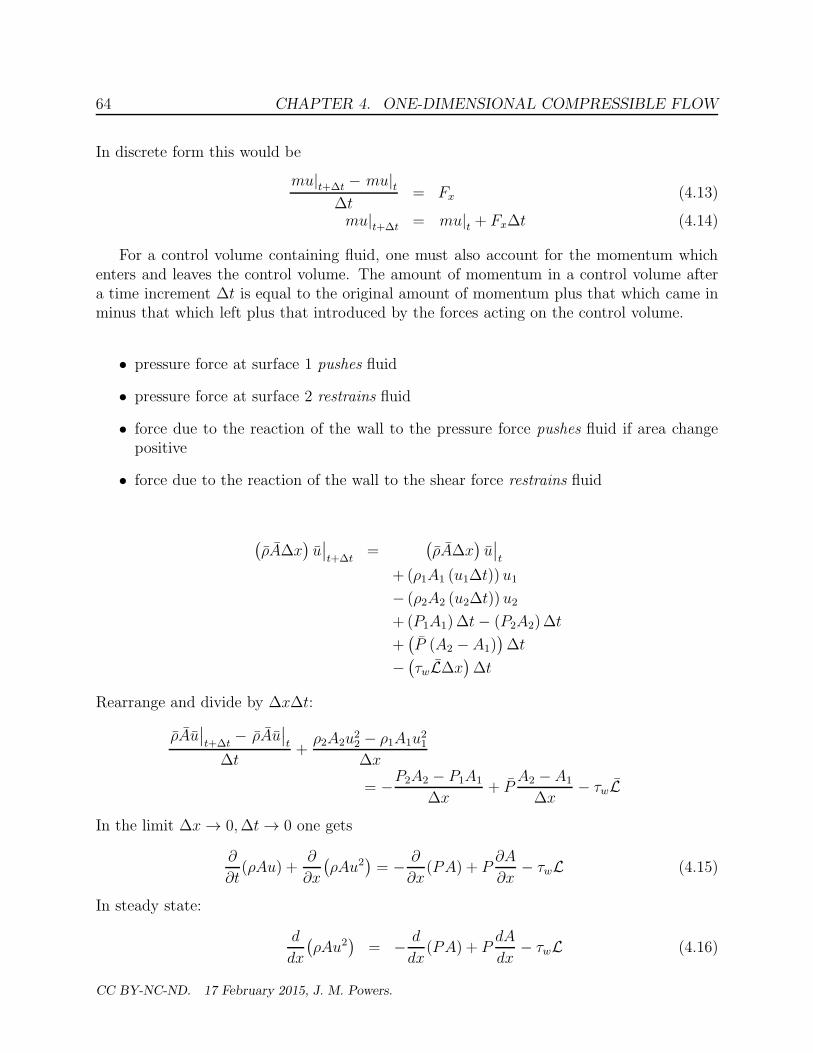
64 CHAPTER 4. ONE-DIMENSIONAL COMPRESSIBLE FLOW
In discrete form this would be
mu|t+∆t − mu|t∆t
= Fx (4.13)
mu|t+∆t = mu|t + Fx∆t (4.14)
For a control volume containing fluid, one must also account for the momentum whichenters and leaves the control volume. The amount of momentum in a control volume aftera time increment ∆t is equal to the original amount of momentum plus that which came inminus that which left plus that introduced by the forces acting on the control volume.
• pressure force at surface 1 pushes fluid
• pressure force at surface 2 restrains fluid
• force due to the reaction of the wall to the pressure force pushes fluid if area changepositive
• force due to the reaction of the wall to the shear force restrains fluid
(
ρA∆x)
u∣
∣
t+∆t=
(
ρA∆x)
u∣
∣
t
+ (ρ1A1 (u1∆t)) u1
− (ρ2A2 (u2∆t)) u2
+ (P1A1)∆t− (P2A2)∆t
+(
P (A2 −A1))
∆t
−(
τwL∆x)
∆t
Rearrange and divide by ∆x∆t:
ρAu∣
∣
t+∆t− ρAu
∣
∣
t
∆t+
ρ2A2u22 − ρ1A1u
21
∆x
= −P2A2 − P1A1
∆x+ P
A2 −A1
∆x− τwL
In the limit ∆x → 0,∆t → 0 one gets
∂
∂t(ρAu) +
∂
∂x
(
ρAu2)
= − ∂
∂x(PA) + P
∂A
∂x− τwL (4.15)
In steady state:
d
dx
(
ρAu2)
= − d
dx(PA) + P
dA
dx− τwL (4.16)
CC BY-NC-ND. 17 February 2015, J. M. Powers.

4.1. GENERALIZED ONE-DIMENSIONAL EQUATIONS 65
ρAudu
dx+ u
d
dx(ρAu) = −P
dA
dx− A
dP
dx+ P
dA
dx− τwL (4.17)
ρudu
dx= −dP
dx− τw
LA
(4.18)
ρudu+ dP = −τwLAdx (4.19)
du+1
ρudP = −τw
Lmdx (4.20)
ρd
(
u2
2
)
+ dP = −τwLAdx (4.21)
Wall shear lowers the combination of pressure and dynamic head.
If no wall shear:
dP = −ρd
(
u2
2
)
(4.22)
Increase in velocity magnitude decreases the pressure.
If no area change dA = 0 and no friction τw ≡ 0:
ρudu
dx+
dP
dx= 0 (4.23)
add u mass ud
dx(ρu) = 0 (4.24)
d
dx
(
ρu2 + P)
= 0 (4.25)
ρu2 + P = ρou2o + Po = C2 (4.26)
4.1.3 Energy
The first law of thermodynamics states that the change of total energy of a body equals theheat transferred to the body minus the work done by the body:
E2 − E1 = Q−W (4.27)
E2 = E1 +Q−W (4.28)
So for the control volume this becomes the following when one also accounts for the energyflux in and out of the control volume in addition to the work and heat transfer:
(
ρA∆x)
(
e+u2
2
)∣
∣
∣
∣
t+∆t
=(
ρA∆x)
(
e+u2
2
)∣
∣
∣
∣
t
+ρ1A1 (u1∆t)
(
e1 +u21
2
)
− ρ2A2 (u2∆t)
(
e2 +u22
2
)
+qw(
L∆x)
∆t+ (P1A1) (u1∆t)− (P2A2) (u2∆t)
CC BY-NC-ND. 17 February 2015, J. M. Powers.
66 CHAPTER 4. ONE-DIMENSIONAL COMPRESSIBLE FLOW
Note:
• mean pressure times area difference does no work because acting on stationary bound-ary
• work done by shear force not included1
Rearrange and divide by ∆t∆x:
ρA(
e + u2
2
)∣
∣
∣
t+∆t− ρA
(
e+ u2
2
)∣
∣
∣
t
∆t
+ρ2A2u2
(
e2 +u22
2+ P2
ρ2
)
− ρ1A1u1
(
e1 +u21
2+ P1
ρ1
)
∆x= qwL
In differential form as ∆x → 0,∆t → 0
∂
∂t
(
ρA
(
e+u2
2
))
+∂
∂x
(
ρAu
(
e+u2
2+
P
ρ
))
= qwL
In steady state:
d
dx
(
ρAu
(
e+u2
2+
P
ρ
))
= qwL (4.29)
ρAud
dx
(
e+u2
2+
P
ρ
)
+
(
e +u2
2+
P
ρ
)
d
dx(ρAu) = qwL (4.30)
ρud
dx
(
e+u2
2+
P
ρ
)
=qwLA
(4.31)
ρu
(
de
dx+ u
du
dx+
1
ρ
dP
dx− P
ρ2dρ
dx
)
=qwLA
(4.32)
subtract product of momentum and velocity (4.33)
ρu2du
dx+ u
dP
dx= −τwLu
A(4.34)
ρude
dx− Pu
ρ
dρ
dx=
qwLA
+τwLuA
(4.35)
de
dx− P
ρ2dρ
dx=
(qw + τwu)Lm
(4.36)
1In neglecting work done by the wall shear force, I have taken an approach which is nearly universal, butfundamentally difficult to defend. At this stage of the development of these notes, I am not ready to enterinto a grand battle with all established authors and probably confuse the student; consequently, results forflow with friction will be consistent with those of other sources. The argument typically used to justify thisis that the real fluid satisfies no-slip at the boundary; thus, the wall shear actually does no work. However,one can easily argue that within the context of the one-dimensional model which has been posed that theshear force behaves as an external force which reduces the fluid’s mechanical energy. Moreover, it is possibleto show that neglect of this term results in the loss of frame invariance, a serious defect indeed. To modelthe work of the wall shear, one would include the term
(
τw(
L∆x))
(u∆t) in the energy equation.
CC BY-NC-ND. 17 February 2015, J. M. Powers.

4.1. GENERALIZED ONE-DIMENSIONAL EQUATIONS 67
Since e = e(P, ρ)
de =∂e
∂ρ
∣
∣
∣
∣
P
dρ+∂e
∂P
∣
∣
∣
∣
ρ
dP (4.37)
de
dx=
∂e
∂ρ
∣
∣
∣
∣
P
dρ
dx+
∂e
∂P
∣
∣
∣
∣
ρ
dP
dx(4.38)
so
∂e
∂ρ
∣
∣
∣
∣
P
dρ
dx+
∂e
∂P
∣
∣
∣
∣
ρ
dP
dx− P
ρ2dρ
dx=
(qw + τwu)Lm
(4.39)
dP
dx+
∂e∂ρ
∣
∣
∣
P− P
ρ2
∂e∂P
∣
∣
ρ
dρ
dx=
(qw + τwu)Lm ∂e
∂P
∣
∣
ρ
(4.40)
Now it can be shown that
c2 =∂P
∂ρ
∣
∣
∣
∣
s
= −
∂e∂ρ
∣
∣
∣
P− P
ρ2
∂e∂P
∣
∣
ρ
(4.41)
so
dP
dx− c2
dρ
dx=
(qw + τwu)Lm ∂e
∂P
∣
∣
ρ
(4.42)
dP
dx− c2
dρ
dx=
(qw + τwu)LρuA ∂e
∂P
∣
∣
ρ
(4.43)
Special case of flow with no heat transfer qw ≡ 0. Area change allowed!, wall frictionallowed! (see earlier footnote):
ρud
dx
(
e+u2
2+
P
ρ
)
= 0 (4.44)
e+u2
2+
P
ρ= eo +
u2o
2+
Po
ρo= C3 (4.45)
h +u2
2= ho +
u2o
2= C3 (4.46)
Example 4.1Adiabatic Flow of Argon2
2adopted from White’s 9.1, p. 583
CC BY-NC-ND. 17 February 2015, J. M. Powers.

68 CHAPTER 4. ONE-DIMENSIONAL COMPRESSIBLE FLOW
Given: Argon, γ = 53 , flows adiabatically through a duct. At section 1, P1 = 200 psia, T1 =
500◦F, u1 = 250 fts . At section 2 P2 = 40 psia, u2 = 1, 100 ft
s .
Find: T2 in ◦F and s2 − s1 in Btulbm◦R
Assume: Ar is a calorically perfect ideal gas, tables give R = 38.68 ft lbflbmR , cp = 0.1253 Btu
lbmR
Analysis: First get the units into shape:
T1 = 500 + 460 = 960 R (4.47)
cp =
(
0.1253Btu
lbm R
)(
779ft lbf
Btu
)(
32.17lbm ft
lbf s2
)
= 3, 140ft2
s2 R(4.48)
R =
(
38.68ft lbf
lbm R
)(
32.17lbm ft
lbf s2
)
= 1, 244ft2
s2 R(4.49)
R =
(
38.68ft lbf
lbm R
)(
1
779
Btu
ft lbf
)
= 0.04965Btu
lbm R(4.50)
Now consider an energy balance:
h2 +u22
2= h1 +
u21
2(4.51)
cpT2 + ho +u22
2= cpT1 + ho +
u21
2(4.52)
T2 = T1 +1
2cp
(
u21 − u2
2
)
(4.53)
T2 = 960 R+1
2
1
3, 140 ft2
s2R
(
(
250ft
s
)2
−(
1, 100ft
s
)2)
= 777 R (4.54)
T2 = 777− 460 = 317◦F (4.55)
The flow sped up; temperature went down. Thermal energy was converted into kinetic energy
Calculate the entropy change. For the calorically perfect ideal gas:
s2 − s1 = cp ln
(
T2
T1
)
−R ln
(
P2
P1
)
(4.56)
= 0.1253Btu
lbm Rln
(
777 R
960 R
)
− 0.04965Btu
lbm Rln
(
40 psia
200 psia
)
(4.57)
= −0.0265− (−.0799) = 0.0534Btu
lbm R(4.58)
Entropy change positive. Since adiabatic, there must have been irreversible friction which gave rise tothis.
Example 4.2Adiabatic Flow of Steam3
3adopted from White’s 9.2, p. 583
CC BY-NC-ND. 17 February 2015, J. M. Powers.

4.1. GENERALIZED ONE-DIMENSIONAL EQUATIONS 69
Same problem now with steam Given: Steam flows adiabatically through a duct. At section 1,P1 = 200 psia, T1 = 500◦F, u1 = 250 ft
s . At section 2 P2 = 40 psia, u2 = 1, 100 fts .
Find: T2 in ◦F and s2 − s1 in Btulbm◦R
Analysis:
Use steam tables for property values.
Energy balance:
h2 +u22
2= h1 +
u21
2(4.59)
h2 = h1 +1
2
(
u21 − u2
2
)
(4.60)
h2 = 1269Btu
lbm+
1
2
(
1
779
Btu
ft lbf
)(
1
32.17
lbf s2
lbm ft
)
(
(
250ft
s
)2
−(
1, 100ft
s
)2)
(4.61)
h2 = 1, 246Btu
lbm(4.62)
Interpolate steam tables at P2 = 40 psia, h2 = h2 = 1, 246 Btulbm and find
T2 = 420◦F (4.63)
s2 = 1.7720Btu
lbm R(4.64)
Tables give s1 = 1.6239 Btulbm R so the entropy change is
s2 − s1 = 1.7720− 1.6239 = 0.148Btu
lbm R(4.65)
Example 4.3Flow of Air with Heat Addition
Given: Air initially at P1 = 100 kPa, T1 = 300 K, u1 = 10 ms flows in a duct of length 100 m.
The duct has a constant circular cross sectional area of A = 0.02 m2 and is isobarically heated witha constant heat flux qw along the entire surface of the duct. At the end of the duct the flow hasP2 = 100 kPa, T2 = 500 K
Find: the mass flow rate m, the wall heat flux qw and the entropy change s2 − s1; check forsatisfaction of the second law.
Assume: Calorically perfect ideal gas, R = 0.287 kJkg K , cp = 1.0035 kJ
kg K
Analysis:
CC BY-NC-ND. 17 February 2015, J. M. Powers.

70 CHAPTER 4. ONE-DIMENSIONAL COMPRESSIBLE FLOW
Geometry:
A = πr2 (4.66)
r =
√
A
π(4.67)
L = 2πr = 2√πA = 2
√
π (0.02 m2) = 0.501 m (4.68)
Get the mass flux.
P1 = ρ1RT1 (4.69)
ρ1 =P1
RT1=
100 kPa(
0.287 kJkg K
)
(300 K)(4.70)
= 1.161kg
m3(4.71)
So
m = ρ1u1A1 =
(
1.161kg
m3
)
(
10m
s
)
(
0.02 m2)
= 0.2322kg
s(4.72)
Get the flow variables at state 2:
ρ2 =P2
RT2=
100 kPa(
0.287 kJkg K
)
(500 K)(4.73)
= 0.6969kg
m3(4.74)
ρ2u2A2 = ρ1u1A1 (4.75)
u2 =ρ1u1A1
ρ2A2=
ρ1u1
ρ2(4.76)
=
(
1.161 kgm3
)
(
10 ms
)
0.6969 kgm3
= 16.67m
s(4.77)
Now consider the energy equation:
ρud
dx
(
e+u2
2+
P
ρ
)
=qwLA
(4.78)
d
dx
(
h+u2
2
)
=qwLm
(4.79)
∫ L
0
d
dx
(
h+u2
2
)
dx =
∫ L
0
qwLm
dx (4.80)
h2 +u22
2− h1 −
u21
2=
qwLLm
(4.81)
cp (T2 − T1) +u22
2− u2
1
2=
qwLLm
(4.82)
qw =
(
m
LL
)(
cp (T2 − T1) +u22
2− u2
1
2
)
(4.83)
(4.84)
CC BY-NC-ND. 17 February 2015, J. M. Powers.

4.1. GENERALIZED ONE-DIMENSIONAL EQUATIONS 71
Substituting the numbers, one finds,
qw =
(
0.2322 kgs
(100 m) (0.501 m)
)(
1, 003.5J
kg K(500 K − 300 K) +
(
16.67 ms
)2
2−(
10 ms
)2
2
)
(4.85)
qw = 0.004635kg
m2 s
(
200, 700J
kg− 88.9
m2
s2
)
(4.86)
qw = 0.004635kg
m2 s
(
200, 700J
kg− 88.9
J
kg
)
(4.87)
qw = 930W
m2(4.88)
Heat flux positive, denoting heat into the air.
Now find the entropy change.
s2 − s1 = cp ln
(
T2
T1
)
−R ln
(
P2
P1
)
(4.89)
s2 − s1 =
(
1, 003.5J
kg K
)
ln
(
500 K
300 K
)
−(
287J
kg K
)
ln
(
100 kPa
100 kPa
)
(4.90)
s2 − s1 = 512.6− 0 = 512.6J
kg K(4.91)
Is the second law satisfied? Assume the heat transfer takes place from a reservoir held at 500 K. Thereservoir would have to be at least at 500 K in order to bring the fluid to its final state of 500 K. Itcould be greater than 500 K and still satisfy the second law.
S2 − S1 ≥ Q12
T(4.92)
S2 − S1 ≥ Q12
T(4.93)
m (s2 − s1) ≥ Q12
T(4.94)
m (s2 − s1) ≥ qwAtot
T(4.95)
m (s2 − s1) ≥ qwLLT
(4.96)
s2 − s1 ≥ qwLLmT
(4.97)
512.6J
kg K≥
(
930 Js m2
)
(100 m) (0.501 m)(
0.2322 kgs
)
(500 K)(4.98)
512.6J
kg K≥ 401.3
J
kg K(4.99)
CC BY-NC-ND. 17 February 2015, J. M. Powers.

72 CHAPTER 4. ONE-DIMENSIONAL COMPRESSIBLE FLOW
4.1.4 Influence coefficients
Now, uncouple these equations. First, summarize:
udρ
dx+ ρ
du
dx= −ρu
A
dA
dx(4.100)
ρudu
dx+
dP
dx= −τwL
A(4.101)
dP
dx− c2
dρ
dx=
(qw + τwu)LρuA ∂e
∂P
∣
∣
ρ
(4.102)
In matrix form this is
u ρ 00 ρu 1
−c2 0 1
dρdxdudxdPdx
=
−ρuA
dAdx
− τwLA
(qw+τwu)LρuA ∂e
∂P |ρ
(4.103)
Use Cramer’s Rule to solve for the derivatives. First calculate the determinant of the coef-ficient matrix:
u ((ρu)(1)− (1)(0))− ρ(
(0)(1)− (−c2)(1))
= ρ(
u2 − c2)
(4.104)
Implementing Cramer’s Rule:
dρ
dx=
ρu(
−ρuA
dAdx
)
− ρ(
− τwLA
)
+ ρ
(
(qw+τwu)LρuA ∂e
∂P |ρ
)
ρ (u2 − c2)(4.105)
du
dx=
−c2(
−ρuA
dAdx
)
+ u(
− τwLA
)
− u
(
(qw+τwu)LρuA ∂e
∂P |ρ
)
ρ (u2 − c2)(4.106)
dP
dx=
ρuc2(
−ρuA
dAdx
)
− ρc2(
− τwLA
)
+ ρu2
(
(qw+τwu)LρuA ∂e
∂P |ρ
)
ρ (u2 − c2)(4.107)
Simplify
dρ
dx=
1
A
−ρu2 dAdx
+ τwL+ (qw+τwu)Lρu ∂e
∂P |ρ(u2 − c2)
(4.108)
du
dx=
1
A
c2ρudAdx
− uτwL − (qw+τwu)Lρ ∂e
∂P |ρρ (u2 − c2)
(4.109)
dP
dx=
1
A
−c2ρu2 dAdx
+ c2τwL+ (qw+τwu)Luρ ∂e
∂P |ρ(u2 − c2)
(4.110)
Note:
CC BY-NC-ND. 17 February 2015, J. M. Powers.

4.2. FLOW WITH AREA CHANGE 73
• a system of coupled non-linear ordinary differential equations
• in standard form for dynamic system analysis: dudx
= f(u)
• valid for general equations of state
• singular when velocity sonic u = c
4.2 Flow with area change
This section will consider flow with area change with an emphasis on isentropic flow. Someproblems will involve non-isentropic flow but a detailed discussion of such flows will bedelayed.
4.2.1 Isentropic Mach number relations
Take special case of
• τw = 0
• qw = 0
• calorically perfect ideal gas (CPIG)
Then
d
dx(ρuA) = 0 (4.111)
d
dx
(
ρu2 + P)
= 0 (4.112)
d
dx
(
e +u2
2+
P
ρ
)
= 0 (4.113)
Integrate the energy equation with h = e+ P/ρ
h+u2
2= ho +
u2o
2(4.114)
If one defines the “o” condition to be a condition of rest, then uo ≡ 0. This is a stagnationcondition. So
h +u2
2= ho (4.115)
(h− ho) +u2
2= 0 (4.116)
CC BY-NC-ND. 17 February 2015, J. M. Powers.

74 CHAPTER 4. ONE-DIMENSIONAL COMPRESSIBLE FLOW
Since CPIG,
cp (T − To) +u2
2= 0 (4.117)
T − To +u2
2cp= 0 (4.118)
1− To
T+
u2
2cpT= 0 (4.119)
Now note that
cp = cpcp − cvcp − cv
=cpcv
cp − cvcpcv
− 1=
γR
γ − 1(4.120)
so
1− To
T+
γ − 1
2
u2
γRT= 0 (4.121)
To
T= 1 +
γ − 1
2
u2
γRT(4.122)
Recall the sound speed and Mach number for a CPIG:
c2 = γRT if P = ρRT, e = cvT + eo (4.123)
M2 ≡(u
c
)2
(4.124)
thus,
To
T= 1 +
γ − 1
2M2 (4.125)
T
To=
(
1 +γ − 1
2M2
)−1
(4.126)
Now if the flow is isentropic one has
T
To=
(
ρ
ρo
)γ−1
=
(
P
Po
)γ−1
γ
(4.127)
Thus
ρ
ρo=
(
1 +γ − 1
2M2
)− 1
γ−1
(4.128)
P
Po=
(
1 +γ − 1
2M2
)− γγ−1
(4.129)
CC BY-NC-ND. 17 February 2015, J. M. Powers.

4.2. FLOW WITH AREA CHANGE 75
For air γ = 7/5 so
T
To=
(
1 +1
5M2
)−1
(4.130)
ρ
ρo=
(
1 +1
5M2
)− 5
2
(4.131)
P
Po
=
(
1 +1
5M2
)− 7
2
(4.132)
Figures 4.2, 4.3 4.4 show the variation of T , ρ and P with M2 for isentropic flow.
Other thermodynamic properties can be determined from these, e.g. sound speed:
c
co=
√
γRT
γRTo
=
√
T
To
=
(
1 +γ − 1
2M2
)−1/2
(4.133)
calorically perfect
ideal gas
R = 0.287 kJ/(kg K)
γ = 7/5
stagnation temperature = 300 K
0 2 4 6 8 10M2
50
100
150
200
250
300
T(K)
Figure 4.2: Static temperature versus Mach number squared
calorically perfect
ideal gas
R = 0.287 kJ/(kg K)
γ = 7/5
stagnation pressure = 1 bar
0 2 4 6 8 10M2
0.2
0.4
0.6
0.8
1
P(bar)
Figure 4.3: Static pressure versus Mach number squared
Example 4.4Airplane problem
CC BY-NC-ND. 17 February 2015, J. M. Powers.

76 CHAPTER 4. ONE-DIMENSIONAL COMPRESSIBLE FLOW
0 2 4 6 8 10M2
0.2
0.4
0.6
0.8
1
1.2
ρ(kg/m3)
calorically perfect ideal gas R = 0.287 kJ/(kg K)
γ = 7/5
stagnation density = 1.16 kg/m3
Figure 4.4: Static density versus Mach number squared
Given: An airplane is flying into still air at u = 200 m/s. The ambient air is at 288 K and101.3 kPa.
Find: Temperature, pressure, and density at nose of airplane
Assume: Steady isentropic flow of CPIG
Analysis: In the steady wave frame, the ambient conditions are static while the nose conditions arestagnation.
M =u
c=
u√γRT
=200 m/s
√
75
(
287 JkgK
)
288 K
= 0.588 (4.134)
so
To = T
(
1 +1
5M2
)
, (4.135)
= (288 K)
(
1 +1
50.5882
)
, (4.136)
= 307.9 K (4.137)
ρo = ρ
(
1 +1
5M2
)52
(4.138)
=101.3 kPa
0.287 kJkgK 288 K
(
1 +1
50.5882
)52
, (4.139)
= 1.45 kg/m3 (4.140)
Po = P
(
1 +1
5M2
)72
, (4.141)
= (101.3 kPa)
(
1 +1
50.5882
)72
(4.142)
= 128 kPa (4.143)
Note the temperature, pressure, and density all rise in the isentropic process. In this wave frame, thekinetic energy of the flow is being converted isentropically to thermal energy.
CC BY-NC-ND. 17 February 2015, J. M. Powers.

4.2. FLOW WITH AREA CHANGE 77
Example 4.5Pressure measurement in compressible flows4
See Figure 4.5.
Air at 100 F
123456789011234567890112345678901123456789011234567890112345678901123456789011234567890112345678901123456789011234567890112345678901123456789011234567890112345678901123456789011234567890112345678901123456789011234567890112345678901123456789011234567890112345678901123456789011234567890112345678901123456789011234567890112345678901123456789011234567890112345678901123456789011234567890112345678901123456789011234567890112345678901123456789011234567890112345678901
123456789012345678901234567890121234567890123456789012345678901212345678901234567890123456789011234567890123456789012345678901212345678901234567890123456789012123456789012345678901234567890112345678901234567890123456789012123456789012345678901234567890121234567890123456789012345678901123456789012345678901234567890121234567890123456789012345678901212345678901234567890123456789011234567890123456789012345678901212345678901234567890123456789012123456789012345678901234567890112345678901234567890123456789012123456789012345678901234567890121234567890123456789012345678901123456789012345678901234567890121234567890123456789012345678901212345678901234567890123456789011234567890123456789012345678901212345678901234567890123456789012123456789012345678901234567890112345678901234567890123456789012123456789012345678901234567890121234567890123456789012345678901123456789012345678901234567890121234567890123456789012345678901212345678901234567890123456789011234567890123456789012345678901212345678901234567890123456789012123456789012345678901234567890112345678901
12345678901123456789011234567890112345678901123456789011234567890112345678901123456789011234567890112345678901
Mercury
8 inches Stagnation State "o"
Static State "1"
z g
Figure 4.5: Compressible pitot tube sketch
Given: Air at u = 750 fts , Mercury manometer which reads a change in height of 8 inches.
Find: Static pressure of air in psia
Assume: Ideal gas behavior for air
Analysis:
First consider the manometer which is governed by fluid statics. In fluid statics, there is no motion,thus there are no viscous forces or fluid inertia; one thus has a balance between surface and body forces.Consider the linear momentum equation:
ρdv
dt= −∇P + ρHgg +∇ · τ (4.144)
0 = −∇P + ρHgg (4.145)
dP
dz= ρHggz (4.146)
P1 − Po = ρHggz (z1 − zo) (4.147)
P1 − Po =
(
845.9lbm
ft3
)(
1
32.2
lbf s2
ft lbm
)(
−32.2ft
s2
)
(0 in− (−8 in))
(
1
12
ft
in
)
(4.148)
P1 − Po = −563.9lbf
ft2(4.149)
Po − P1 = 563.9lbf
ft2(4.150)
Po = P1 + 563.9lbf
ft2(4.151)
4adopted from White, 9.26, p. 584
CC BY-NC-ND. 17 February 2015, J. M. Powers.

78 CHAPTER 4. ONE-DIMENSIONAL COMPRESSIBLE FLOW
Now calculate the local Mach number
T1 = 100 + 460 = 560 R (4.152)
M1 =u1√γRT1
(4.153)
M1 =750 ft
s√
(1.4)(
1, 717 ft2
s2 R
)
(560 R)
(4.154)
M1 = 0.646 (4.155)
Isentropic flow relations relate stagnation to static properties, so for air
Po = P1
(
1 +1
5M2
1
)3.5
(4.156)
Po = P1
(
1 +1
5(0.646)
2
)3.5
(4.157)
Po = 1.324P1 (4.158)
Substituting from the measured pressure difference
P1 + 563.9lbf
ft2= 1.324P1 (4.159)
−0.324P1 = −563.9lbf
ft2(4.160)
P1 =−563.9 lbf
ft2
−0.324(4.161)
P1 = 1, 740lbf
ft2(4.162)
Po = (1.324)
(
1, 740lbf
ft2
)
= 2, 304lbf
ft2(4.163)
P1 =
(
1, 740lbf
ft2
)(
1
12
ft
in
)2
= 12.1 psia (4.164)
Po =
(
2, 304lbf
ft2
)(
1
12
ft
in
)2
= 16.0 psia (4.165)
What might one estimate if one did not account for compressibility effects? Assume one had thesame static pressure and calculate what velocity one would predict.
First calculate the static density.
ρ1 =P1
RT1(4.166)
ρ1 =1, 740 lbf
ft2(
1, 717 ft2
s2 R
)
(560 R)
(
32.2ft lbm
lbf s2
)
(4.167)
ρ1 = 0.05827lbm
ft3(4.168)
CC BY-NC-ND. 17 February 2015, J. M. Powers.

4.2. FLOW WITH AREA CHANGE 79
One would then use an incompressible Bernoulli equation:
Po +ρ (0)
2
2= P1 +
ρ1u21
2(4.169)
u1 =
√
2 (Po − P1)
ρ1(4.170)
u1 =
√
√
√
√
√
2(
563.9 lbfft2
)
0.05827 lbmft3
(
32.2ft lbm
lbf s2
)
(4.171)
u1 = 789.4ft
s(4.172)
So the relative error in using the incompressible approximation would be
Error =789.4− 750
750= 5.3% (4.173)
Example 4.6Adiabatic Duct Flow5
Given: Air flowing adiabatically through a duct. At section 1, u1 = 400 fts , T1 = 200◦F, P1 =
35 psia. Downstream u2 = 1, 100 fts , P2 = 18 psia.
Find: M2, umax,Po2
Po1
Assume: Calorically perfect ideal gas, steady, one-dimensional flow
Analysis:
Some preliminaries:
T1 = 200 + 460 = 660 R (4.174)
cp =
(
0.240Btu
lbm R
)(
779ft lbf
Btu
)(
32.17lbm ft
lbf s2
)
= 6, 015ft2
s2 R(4.175)
R =
(
53.34ft lbf
lbm R
)(
32.17lbm ft
lbf s2
)
= 1, 716ft2
s2 R(4.176)
(4.177)
Energy conservation gives stagnation conditions at state 1
h1 +u21
2= ho1 (4.178)
5adopted from White’s 9.30, p. 585
CC BY-NC-ND. 17 February 2015, J. M. Powers.

80 CHAPTER 4. ONE-DIMENSIONAL COMPRESSIBLE FLOW
cpT1 +u21
2= cpTo1 (4.179)
To1 = T1 +u21
2cp(4.180)
To1 = 660 R+
(
400 fts
)2
2(
6, 015 ft2
s2 R
) (4.181)
To1 = 673 R (4.182)
Note since in adiabatic flow ho is a constant, ho2 = ho1 and since ideal gas To2 = To1 So
To2 = 673 R (4.183)
T2 = To2 −u22
2cp(4.184)
T2 = 673 R−
(
1, 100 fts
)2
2(
6, 015 ft2
s2 R
) (4.185)
T2 = 572 R (4.186)
Calculate the Mach numbers:
c1 =√
γRT1 (4.187)
c1 =
√
1.4
(
1, 716ft2
s2 R
)
(660 R) = 1, 259ft
s(4.188)
M1 =u1
c1=
400 fts
1, 259 fts
= 0.318 (4.189)
c2 =√
γRT2 (4.190)
c2 =
√
1.4
(
1, 716ft2
s2 R
)
(572 R) = 1, 173ft
s(4.191)
M2 =u2
c2=
1, 100 fts
1, 173 fts
= 0.938 (4.192)
Since for CPIG air one has
P
Po=
(
1 +1
5M2
)
−72
(4.193)
Po = P
(
1 +1
5M2
)72
(4.194)
Po1 = (35 psia)
(
1 +1
50.3182
)72
= 37.54 psia (4.195)
Po2 = (18 psia)
(
1 +1
50.9382
)72
= 31.74 psia (4.196)
Po2
Po1=
31.74 psia
37.54 psia= 0.845 (4.197)
CC BY-NC-ND. 17 February 2015, J. M. Powers.

4.2. FLOW WITH AREA CHANGE 81
Stagnation pressure drop indicates that friction was present. If one computed an entropy change onewould see an increase in entropy.
The maximum velocity is found by converting all the thermal energy to kinetic energy. Takingzero thermal energy to correspond to absolute zero (despite the fact that air would not be a gas at thispoint) one could estimate
ho =u2max
2(4.198)
cpTo =u2max
2(4.199)
umax =√
2cpTo (4.200)
umax =
√
2
(
6, 015ft2
s2 R
)
(673 R) = 2, 845ft
s(4.201)
4.2.2 Sonic properties
Let “*” denote a property at the sonic state M2 ≡ 1
T∗
To=
(
1 +γ − 1
212)−1
=2
γ + 1(4.202)
ρ∗ρo
=
(
1 +γ − 1
212)− 1
γ−1
=
(
2
γ + 1
)1
γ−1
(4.203)
P∗
Po=
(
1 +γ − 1
212)− γ
γ−1
=
(
2
γ + 1
)γ
γ−1
(4.204)
c∗co
=
(
1 +γ − 1
212)−1/2
=
√
2
γ + 1(4.205)
u∗ = c∗ =√
γRT∗ =
√
2γ
γ + 1RTo (4.206)
If air γ = 7/5 and
T∗
To= 0.8333 (4.207)
ρ∗ρo
= 0.6339 (4.208)
P∗
Po
= 0.5283 (4.209)
c∗co
= 0.9123 (4.210)
CC BY-NC-ND. 17 February 2015, J. M. Powers.

82 CHAPTER 4. ONE-DIMENSIONAL COMPRESSIBLE FLOW
4.2.3 Effect of area change
Influence of mass equation must be considered. So far only looked at energy has beenexamined. In the isentropic limit the mass, momentum, and energy equation for a CPIGreduce to
dρ
ρ+
du
u+
dA
A= 0 (4.211)
ρudu+ dP = 0 (4.212)
dP
P= γ
dρ
ρ(4.213)
Substitute energy then mass into momentum:
ρudu+ γP
ρdρ = 0 (4.214)
ρudu+ γP
ρ
(
−ρ
udu− ρ
AdA)
= 0 (4.215)
du+ γP
ρ
(
− 1
u2du− 1
uAdA
)
= 0 (4.216)
du
(
1− γP/ρ
u2
)
= γP
ρ
dA
uA(4.217)
du
u
(
1− γP/ρ
u2
)
=γP/ρ
u2
dA
A(4.218)
du
u
(
1− 1
M2
)
=1
M2
dA
A(4.219)
du
u
(
M2 − 1)
=dA
A(4.220)
du
u=
1
M2 − 1
dA
A(4.221)
Figure 4.6 gives show the performance of a fluid in a variable area duct.It is noted that
• equation singular when M2 = 1
• if M2 = 1, one needs dA = 0
• area minimum necessary to transition from subsonic to supersonic flow!!
• can be shown area maximum not relevant
Consider A at a sonic state. From the mass equation:
ρuA = ρ∗u∗A∗ (4.222)
CC BY-NC-ND. 17 February 2015, J. M. Powers.
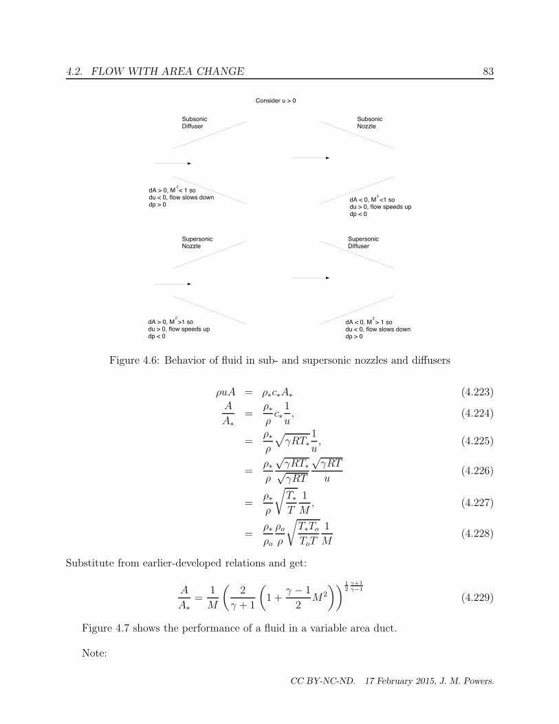
4.2. FLOW WITH AREA CHANGE 83
Consider u > 0
SubsonicDiffuser
SubsonicNozzle
SupersonicNozzle
SupersonicDiffuser
dA > 0, M < 1 sodu < 0, flow slows downdp > 0
2
dA < 0, M <1 sodu > 0, flow speeds updp < 0
2
dA < 0, M > 1 sodu < 0, flow slows downdp > 0
2
dA > 0, M >1 sodu > 0, flow speeds updp < 0
2
Figure 4.6: Behavior of fluid in sub- and supersonic nozzles and diffusers
ρuA = ρ∗c∗A∗ (4.223)
A
A∗=
ρ∗ρc∗1
u, (4.224)
=ρ∗ρ
√
γRT∗1
u, (4.225)
=ρ∗ρ
√γRT∗√γRT
√γRT
u(4.226)
=ρ∗ρ
√
T∗
T
1
M, (4.227)
=ρ∗ρo
ρoρ
√
T∗To
ToT
1
M(4.228)
Substitute from earlier-developed relations and get:
A
A∗=
1
M
(
2
γ + 1
(
1 +γ − 1
2M2
))1
2
γ+1
γ−1
(4.229)
Figure 4.7 shows the performance of a fluid in a variable area duct.
Note:
CC BY-NC-ND. 17 February 2015, J. M. Powers.

84 CHAPTER 4. ONE-DIMENSIONAL COMPRESSIBLE FLOW
0 0.5 1 1.5 2 2.5 3M
1
2
3
4
5
6
A/A*
calorically perfect ideal gas R = 0.287 kJ/(kg K)
γ = 7/5
Figure 4.7: Area versus Mach number for a calorically perfect ideal gas
• AA∗
has a minimum value of 1 at M = 1
• For each AA∗ > 1, there exist two values of M
• AA∗
→ ∞ as M → 0 or M → ∞
4.2.4 Choking
Consider mass flow rate variation with pressure difference
• small pressure difference gives small velocity, small mass flow
• as pressure difference grows, velocity and mass flow rate grow
• velocity is limited to sonic at a particular duct location
• this provides fundamental restriction on mass flow rate
• can be proven rigorously that sonic condition gives maximum mass flow rate
mmax = ρ∗u∗A∗ (4.230)
if ideal gas: = ρo
(
2
γ + 1
)1
γ−1(√
2γ
γ + 1RTo
)
A∗ (4.231)
= ρo
(
2
γ + 1
)1
γ−1(
2
γ + 1
)1/2√
γRToA∗ (4.232)
= ρo
(
2
γ + 1
)1
2
γ+1
γ−1 √
γRToA∗ (4.233)
A flow which has a maximum mass flow rate is known as choked flow. Flows will chokeat area minima in a duct.
CC BY-NC-ND. 17 February 2015, J. M. Powers.

4.2. FLOW WITH AREA CHANGE 85
Example 4.7Isentropic area change problem with choking6
Given: Air with stagnation conditions Po = 200 kPa To = 500 K flows through a throat to an exitMach number of 2.5. The desired mass flow is 3.0 kg/s,
Find: a) throat area, b) exit pressure, c) exit temperature, d) exit velocity, and e) exit area.
Assume: CPIG, isentropic flow, γ = 7/5
Analysis:
ρo =Po
RTo=
200 kPa
(0.287 kJ/kg) (500 K)= 1.394 kg/m3 (4.234)
Since it necessarily flows through a sonic throat:
mmax = ρo
(
2
γ + 1
)12
γ+1
γ−1√
γRToA∗ (4.235)
A∗ =mmax
ρo
(
2γ+1
)12
γ+1
γ−1 √γRTo
(4.236)
=3 kg/s
(
1.394 kgm3
)
(0.5787)
√
1.4(
287 Jkg K
)
(500 K)
, (4.237)
= 0.008297 m2 (4.238)
Since Me is known, use the isentropic relations to find other exit conditions.
Pe = Po
(
1 +γ − 1
2M2
e
)
−γ
γ−1
, (4.239)
= (200 kPa)
(
1 +1
52.52
)
−3.5
, (4.240)
= 11.71 kPa (4.241)
Te = To
(
1 +γ − 1
2M2
e
)
−1
, (4.242)
= (500 K)
(
1 +1
52.52
)
−1
, (4.243)
= 222.2 K (4.244)
Note
ρe =Pe
RTe, (4.245)
=11.71 kPa
(
0.287 kJkgK
)
(222.2 K), (4.246)
= 0.1834kg
m3(4.247)
6adopted from White, Fluid Mechanics McGraw-Hill: New York, 1986, p. 529, Ex. 9.5
CC BY-NC-ND. 17 February 2015, J. M. Powers.

86 CHAPTER 4. ONE-DIMENSIONAL COMPRESSIBLE FLOW
Now the exit velocity is simply
ue = Mece = Me
√
γRTe = 2.5
√
1.4
(
287J
kg K
)
(222.2 K) = 747.0m
s(4.248)
Now determine the exit area:
A =A∗
Me
(
2
γ + 1
(
1 +γ − 1
2M2
e
))12
γ+1
γ−1
(4.249)
=0.008297 m2
2.5
(
5
6
(
1 +1
52.52
))3
, (4.250)
= 70.0219 m2 (4.251)
Example 4.8Discharge Problem7
Given: Air in tank, Po = 700 kPa, To = 20◦C, V = 1.5 m3. Throat area in converging nozzle of0.65 cm2, exhausting to 1 atm environment
Find: Time for pressure in tank to decrease to 500 kPa.
Assume: CPIG, stagnation temperature constant (so small heat transfer to tank in time of opera-tion)
Analysis:First, To = 20 + 273 = 293 K
Now check for choked flow! At the initial state
Patm
Po=
101.3 kPa
700 kPa= 0.145 (4.252)
But for air P∗
Po
= 0.5283, so the flow must be choked at the exit and the mass flow is restricted.(Further expansion takes place outside the nozzle)
For choked flow one has
me = ρo
(
2
γ + 1
)12
γ+1
γ−1√
γRToA∗ (4.253)
=
(
Po
RTo
)(
2
γ + 1
)12
γ+1
γ−1√
γRToA∗ (4.254)
=
Po(
287 Jkg K
)
(293 K)
0.5787
√
1.4
(
287J
kg K
)
(293 K)(
0.65 cm2)
(
1
100
m
cm
)2
(4.255)
= 1.5348× 10⁻⁷Po (4.256)
7from White, 9.33,35
CC BY-NC-ND. 17 February 2015, J. M. Powers.

4.3. NORMAL SHOCK WAVES 87
Now mass conservation gives
d
dtmcv = −me (4.257)
d
dt(ρoV ) = −me (4.258)
d
dt
(
Po
RToV
)
= −me (4.259)
dPo
dt= −RTo
Vme (4.260)
dPo
dt= −
(
287 Jkg K
)
(293 K)
1.5 m31.5348× 10−7Po (4.261)
dPo
dt= −0.008604Po (4.262)
Po = A exp (−0.008604t) (4.263)
Use initial value of Po to fix the constant A so
Po = 700 exp (−0.008604t) (4.264)
When does Po = 500 kPa?
500 = 700 exp (−0.008604t) ln500
700= −0.008604t (4.265)
t = − 1
0.008604ln
500
700= 39.1 s (4.266)
4.3 Normal shock waves
This section will develop relations for normal shock waves in fluids with general equations ofstate. It will be specialized to calorically perfect ideal gases to illustrate the general featuresof the waves.
Assumptions for this section
• one-dimensional flow
• steady flow
• no area change
• viscous effects and wall friction do not have time to influence flow
• heat conduction and wall heat transfer do not have time to influence flow
CC BY-NC-ND. 17 February 2015, J. M. Powers.

88 CHAPTER 4. ONE-DIMENSIONAL COMPRESSIBLE FLOW
Steady Frame
x
u = - D
P1 ρ
1
u2
P2
ρ2
Laboratory Frame
v = 0 P1
ρ1
v = v2 P2
ρ2
vp = v2
D
u = v - D; v = u + D x = x* - D t; x* = x + D t
x*
Figure 4.8: Normal shock sketch
The piston problem as sketched in Figure 4.8 will be considered.Physical problem:
• Drive piston with known velocity vp into fluid at rest (v1 = 0) with known properties,P1, ρ1 in the x∗ laboratory frame
• Determine disturbance speed D
• Determine disturbance properties v2, P2, ρ2
• in this frame of reference unsteady problem
Transformed Problem:
• use Galilean transformation x = x∗−Dt, u = v−D to transform to the frame in whichthe wave is at rest, therefore rending the problem steady in this frame
• solve as though D is known to get downstream “2” conditions: u2(D), P2(D), ...
• invert to solve for D as function of u2, the transformed piston velocity: D(u2)
• back transform to get all variables as function of v2, the laboratory piston velocity:D(v2), P2(v2), ρ2(v2), ...
4.3.1 Governing equations
Under these assumptions the conservation principles in conservative form and equation ofstate are in the steady frame as follows:
d
dx(ρu) = 0 (4.267)
d
dx
(
ρu2 + P)
= 0 (4.268)
CC BY-NC-ND. 17 February 2015, J. M. Powers.
4.3. NORMAL SHOCK WAVES 89
d
dx
(
ρu
(
h+u2
2
))
= 0 (4.269)
h = h(P, ρ) (4.270)
Upstream conditions are ρ = ρ1, P = P1, u = −D. With knowledge of the equation ofstate, one gets h = h1. Integrating the equations from upstream to state “2” gives:
ρ2u2 = −ρ1D (4.271)
ρ2u22 + P2 = ρ1D
2 + P1 (4.272)
h2 +u22
2= h1 +
D2
2(4.273)
h2 = h(P2, ρ2) (4.274)
4.3.2 Rayleigh line
Work on the momentum equation:
P2 = P1 + ρ1D2 − ρ2u
22 (4.275)
P2 = P1 +ρ21D
2
ρ1− ρ22u
22
ρ2(4.276)
Since mass gives ρ22u22 = ρ21D
2 one gets an equation for the Rayleigh Line, a line in (P, 1ρ)
space:
P2 = P1 + ρ21D2
(
1
ρ1− 1
ρ2
)
(4.277)
Note:
• Rayleigh line passes through ambient state
• Rayleigh line has negative slope
• magnitude of slope proportional to square of wave speed
• independent of state and energy equations
4.3.3 Hugoniot curve
Operate on the energy equation, using both mass and momentum to eliminate velocity. Firsteliminate u2 via the mass equation:
CC BY-NC-ND. 17 February 2015, J. M. Powers.

90 CHAPTER 4. ONE-DIMENSIONAL COMPRESSIBLE FLOW
h2 +u22
2= h1 +
D2
2(4.278)
h2 +1
2
(
ρ1D
ρ2
)2
= h1 +D2
2(4.279)
h2 − h1 +D2
2
(
(
ρ1ρ2
)2
− 1
)
= 0 (4.280)
h2 − h1 +D2
2
(
ρ21 − ρ22ρ22
)
= 0 (4.281)
h2 − h1 +D2
2
(
(ρ1 − ρ2) (ρ1 + ρ2)
ρ22
)
= 0 (4.282)
Now use the Rayleigh line to eliminate D2:
D2 = (P2 − P1)
(
1
ρ21
)(
1
ρ1− 1
ρ2
)−1
(4.283)
D2 = (P2 − P1)
(
1
ρ21
)(
ρ2 − ρ1ρ1ρ2
)−1
(4.284)
D2 = (P2 − P1)
(
1
ρ21
)(
ρ1ρ2ρ2 − ρ1
)
(4.285)
so the energy equation becomes
h2 − h1 +1
2(P2 − P1)
(
1
ρ21
)(
ρ1ρ2ρ2 − ρ1
)(
(ρ1 − ρ2) (ρ1 + ρ2)
ρ22
)
= 0 (4.286)
h2 − h1 −1
2(P2 − P1)
(
1
ρ1
)(
ρ1 + ρ2ρ2
)
= 0 (4.287)
h2 − h1 −1
2(P2 − P1)
(
1
ρ2+
1
ρ1
)
= 0 (4.288)
(4.289)
Solving finally for the enthalpy difference, one finds
h2 − h1 = (P2 − P1)
(
1
2
)(
1
ρ2+
1
ρ1
)
(4.290)
This equation is the Hugoniot equation.
• enthalpy change equals pressure difference times mean volume
• independent of wave speed D and velocity u2
• independent of equation of state
CC BY-NC-ND. 17 February 2015, J. M. Powers.

4.3. NORMAL SHOCK WAVES 91
4.3.4 Solution procedure for general equations of state
The shocked state can be determined by the following procedure:
• specify and equation of state h(P, ρ)
• substitute the equation of state into the Hugoniot to get a second relation between P2
and ρ2.
• use the Rayleigh line to eliminate P2 in the Hugoniot so that the Hugoniot is a singleequation in ρ2
• solve for ρ2 as functions of “1” and D
• back substitute to solve for P2, u2, h2, T2 as functions of “1” and D
• invert to find D as function of “1” state and u2
• back transform to laboratory frame to getD as function of “1” state and piston velocityv2 = vp
4.3.5 Calorically perfect ideal gas solutions
Follow this procedure for the special case of a calorically perfect ideal gas.
h = cp(T − To) + ho (4.291)
P = ρRT (4.292)
so
h = cp
(
P
Rρ− Po
Rρo
)
+ ho (4.293)
h =cpR
(
P
ρ− Po
ρo
)
+ ho (4.294)
h =cp
cp − cv
(
P
ρ− Po
ρo
)
+ ho (4.295)
h =γ
γ − 1
(
P
ρ− Po
ρo
)
+ ho (4.296)
Evaluate at states 1 and 2 and substitute into Hugoniot:(
γ
γ − 1
(
P2
ρ2− Po
ρo
)
+ ho
)
−(
γ
γ − 1
(
P1
ρ1− Po
ρo
)
+ ho
)
= (P2 − P1)
(
1
2
)(
1
ρ2+
1
ρ1
)
CC BY-NC-ND. 17 February 2015, J. M. Powers.

92 CHAPTER 4. ONE-DIMENSIONAL COMPRESSIBLE FLOW
γ
γ − 1
(
P2
ρ2− P1
ρ1
)
− (P2 − P1)
(
1
2
)(
1
ρ2+
1
ρ1
)
= 0
P2
(
γ
γ − 1
1
ρ2− 1
2ρ2− 1
2ρ1
)
− P1
(
γ
γ − 1
1
ρ1− 1
2ρ2− 1
2ρ1
)
= 0
P2
(
γ + 1
2 (γ − 1)
1
ρ2− 1
2ρ1
)
− P1
(
γ + 1
2 (γ − 1)
1
ρ1− 1
2ρ2
)
= 0
P2
(
γ + 1
γ − 1
1
ρ2− 1
ρ1
)
− P1
(
γ + 1
γ − 1
1
ρ1− 1
ρ2
)
= 0
P2 = P1
γ+1γ−1
1ρ1
− 1ρ2
γ+1γ−1
1ρ2
− 1ρ1
• a hyperbola in (P, 1ρ) space
• 1ρ2
→ γ−1γ+1
1ρ1
causes P2 → ∞, note = γ = 1.4, ρ2 → 6 for infinite pressure
• as 1ρ2
→ ∞, P2 → −P1γ−1γ+1
, note negative pressure, not physical here
The Rayleigh line and Hugoniot curves are sketched in Figure 4.9.
2 3 4 5 6 7
100
200
300
400
500
1/ρ (kg/m )3
P (kPa)
1/ρ 1
1/ρ 2
P1
P2
initial state
excluded zoneslope of Rayleigh line < 0
excluded zone, 2nd law violation
Hugoniot,from energy
Rayleigh line, slope ~ Dfrom mass and momentum
2
1/ρ = (γ-1) 1 (γ+1) ρ
min
1
-(γ-1) P1
γ+1 excluded zone, negative pressure
shocked state
excludedzone,1/ρ < 1/ρ
min
Figure 4.9: Rayleigh line and Hugoniot curve.
Note:
• intersections of the two curves are solutions to the equations
• the ambient state “1” is one solution
CC BY-NC-ND. 17 February 2015, J. M. Powers.

4.3. NORMAL SHOCK WAVES 93
• the other solution “2” is known as the shock solution
• shock solution has higher pressure and higher density
• higher wave speed implies higher pressure and higher density
• a minimum wavespeed exists
– occurs when Rayleigh line tangent to Hugoniot
– occurs for very small pressure changes
– corresponds to a sonic wave speed
– disturbances are acoustic
• if pressure increases, can be shown entropy increases
• if pressure decreases (wave speed less than sonic), entropy decreases; this is non-physical
Substitute Rayleigh line into Hugoniot to get single equation for ρ2
P1 + ρ21D2
(
1
ρ1− 1
ρ2
)
= P1
γ+1γ−1
1ρ1
− 1ρ2
γ+1γ−1
1ρ2
− 1ρ1
(4.297)
This equation is quadratic in 1ρ2
and factorizable. Use computer algebra to solve and get
two solutions, one ambient 1ρ2
= 1ρ1
and one shocked solution:
1
ρ2=
1
ρ1
γ − 1
γ + 1
(
1 +2γ
(γ − 1)D2
P1
ρ1
)
(4.298)
The shocked density ρ2 is plotted against wave speed D for CPIG air in Figure 4.10.
Note
• density solution allows allows all wave speeds 0 < D < ∞
• plot range, however, is c1 < D < ∞
• Rayleigh line and Hugoniot show D ≥ c1
• solution for D = D(vp), to be shown, rigorously shows D ≥ c1
• strong shock limit: D2 → ∞, ρ2 → γ+1γ−1
• acoustic limit: D2 → γ P1
ρ1, ρ2 → ρ1
• non-physical limit: D2 → 0, ρ2 → 0
CC BY-NC-ND. 17 February 2015, J. M. Powers.

94 CHAPTER 4. ONE-DIMENSIONAL COMPRESSIBLE FLOW
strong
shock
limit
calorically perfectideal air
γ = 7/5
R = 0.287 kJ/(kg K)
exact solution
D = Dmin = c1
500 1000 1500 2000 2500 3000D (m/s)
1
2
3
4
5
6
7
ρ2 (kg/m3)
Figure 4.10: Shock density vs. shock wave speed for calorically perfect ideal air.
Back substitute into Rayleigh line and mass conservation to solve for the shocked pressureand the fluid velocity in the shocked wave frame:
P2 =2
γ + 1ρ1D
2 − γ − 1
γ + 1P1 (4.299)
u2 = −Dγ − 1
γ + 1
(
1 +2γ
(γ − 1)D2
P1
ρ1
)
(4.300)
The shocked pressure P2 is plotted against wave speed D for CPIG air in Figure 4.11including both the exact solution and the solution in the strong shock limit. Note for theseparameters, the results are indistinguishable.
calorically perfect
ideal air
γ = 7/5
R = 0.287 kJ/(kg K)
exact solution and strong shock limit
ambient = 100000 Pa
D = Dmin = c1
500 1000 1500 2000 2500 3000D (m/s)
62. 10
64. 10
66. 10
68. 10
P2 (Pa)
x
x
x
x
Figure 4.11: Shock pressure vs. shock wave speed for calorically perfect ideal air.
The shocked wave frame fluid particle velocity u2 is plotted against wave speed D forCPIG air in Figure 4.12.
CC BY-NC-ND. 17 February 2015, J. M. Powers.

4.3. NORMAL SHOCK WAVES 95
strong
shock
limit
γ = 7/5
R = 0.287 kJ/(kg K)
exact solution
u1 = - c1 D = Dmin = c1
500 1000 1500 2000 2500 3000D (m/s)
-500
-400
-300
-200
-100
u2 (m/s)
calorically perfect
ideal air
Figure 4.12: Shock wave frame fluid particle velocity vs. shock wave speed for caloricallyperfect ideal air.
The shocked wave frame fluid particle velocity M22 =
ρ2u22
γP2is plotted against wave speed
D for CPIG air in Figure 4.13.
calorically perfectideal air
γ = 7/5
R = 0.287 kJ/(kg K)
exact solution
strong
shock limit
D = Dmin = c1 M2
2 = 1
0 500 1000 1500 2000 2500 3000D (m/s)
0.2
0.4
0.6
0.8
1
M22
Figure 4.13: Mach number squared of shocked fluid particle vs. shock wave speed for calor-ically perfect ideal air.
Exercise: For the conditions shown in the plot of M22 vs. D do the detailed calculations
to demonstrate the plot is correct.
Note in the steady frame that
• The Mach number of the undisturbed flow is (and must be) > 1: supersonic
• The Mach number of the shocked flow is (and must be) < 1: subsonic
CC BY-NC-ND. 17 February 2015, J. M. Powers.

96 CHAPTER 4. ONE-DIMENSIONAL COMPRESSIBLE FLOW
Transform back to the laboratory frame u = v −D:
v2 −D = −Dγ − 1
γ + 1
(
1 +2γ
(γ − 1)D2
P1
ρ1
)
(4.301)
v2 = D −Dγ − 1
γ + 1
(
1 +2γ
(γ − 1)D2
P1
ρ1
)
(4.302)
Manipulate the above equation and solve the resulting quadratic equation for D and get
D =γ + 1
4v2 ±
√
γP1
ρ1+ v22
(
γ + 1
4
)2
(4.303)
Now if v2 > 0, one expects D > 0 so take positive root, also set velocity equal pistonvelocity v2 = vp
D =γ + 1
4vp +
√
γP1
ρ1+ v2p
(
γ + 1
4
)2
(4.304)
Note:
• acoustic limit: as vp → 0, D → c1; the shock speed approaches the sound speed
• strong shock limit: as vp → ∞, D → γ+12vp
The shock speed D is plotted against piston velocity vp for CPIG air in Figure 4.14. Boththe exact solution and strong shock limit are shown.
200 400 600 800 1000vp (m/s)
200
400
600
800
1000
1200
D (m/s)
exact solution
acoustic limit,
D c1
calorically perfectideal air
γ = 7/5
R = 0.287 kJ/(kg K)
strong
shock
limit
Figure 4.14: Shock speed vs. piston velocity for calorically perfect ideal air.
If the Mach number of the shock is defined as
Ms ≡D
c1(4.305)
CC BY-NC-ND. 17 February 2015, J. M. Powers.

4.3. NORMAL SHOCK WAVES 97
one gets
Ms =γ + 1
4
vp√γRT1
+
√
1 +v2p
γRT1
(
γ + 1
4
)2
(4.306)
The shock Mach number Ms is plotted against piston velocity vp for CPIG air in Figure4.15. Both the exact solution and strong shock limit are shown.
200 400 600 800 1000vp (m/s)
0.5
1
1.5
2
2.5
3
3.5
Ms
strong
shock
limit
exact solution
acoustic limit,
Ms 1
calorically perfect
ideal air
γ = 7/5
R = 0.287 kJ/(kg K)
Figure 4.15: Shock Mach number vs. piston velocity for calorically perfect ideal air
Example 4.9Normal shock problem8
Given: Air flowing through normal shock. Upstream u1 = 600 m/s, To1 = 500 K, Po1 = 700 kPa.
Find: Downstream conditions M2, u2, T2, P2, Po2 and s2 − s1.
Assume: calorically perfect ideal gas
Analysis:First get all local unshocked conditions.
To1 = T1 +u21
2cp(4.307)
T1 = To1 −u21
2cp(4.308)
T1 = 500 K −(
600 ms
)2
2(
1004.5 Jkg K
) , (4.309)
= 320.81 K (4.310)
c1 =√
γRT1, (4.311)
=
√
1.4
(
287J
kg K
)
(320.81 K), (4.312)
= 359.0m
s(4.313)
8adopted from White’s 9.46, p. 586
CC BY-NC-ND. 17 February 2015, J. M. Powers.
98 CHAPTER 4. ONE-DIMENSIONAL COMPRESSIBLE FLOW
M1 =u1
c1, (4.314)
=600 m
s
359.0 ms
, (4.315)
= 1.671 (4.316)
P1 = Po1
(
1 +1
5M2
1
)
−3.5
, (4.317)
= (700 kPa)
(
1 +1
5(1.671)
2
)
−3.5
, (4.318)
= 148.1 kPa (4.319)
ρ1 =P1
RT1, (4.320)
=148.1 kPa
(
0.287 kJkg K
)
(320.81 K), (4.321)
= 1.609kg
m3(4.322)
A1
A1∗=
1
M1
(
2
γ + 1
(
1 +γ − 1
2M2
1
))12
γ+1
γ−1
(4.323)
=1
1.671
(
2
1.4 + 1
(
1 +1.4− 1
21.6712
))12
1.4+1
1.4−1
, (4.324)
= 1.311 (4.325)
Now in this case it is fortunate because the incoming velocity D = 600 ms is known. Note that the
shock density only depends on D2, so one can be a little sloppy here with sign. Solve for the shockedstate:
1
ρ2=
1
ρ1
γ − 1
γ + 1
(
1 +2γ
(γ − 1)D2
P1
ρ1
)
(4.326)
1
ρ2=
1
1.609 kgm3
1.4− 1
1.4 + 1
(
1 +2 (1.4)
(1.4− 1)(
600 ms
)2
148, 100 Pa
1.609 kgm3
)
(4.327)
= 0.2890m3
kg(4.328)
ρ2 =1
0.2890 m3
kg
, (4.329)
= 3.461kg
m3(4.330)
Now a variety of equations can be used to determine the remaining state variables. Mass gives u2:
ρ2u2 = ρ1u1 (4.331)
u2 =ρ1u1
ρ2, (4.332)
=
(
1.609 kgm3
)
(
600 ms
)
3.461 kgm3
, (4.333)
CC BY-NC-ND. 17 February 2015, J. M. Powers.

4.3. NORMAL SHOCK WAVES 99
= 278.9m
s. (4.334)
Momentum gives P2
P2 + ρ2u22 = P1 + ρ1u
21 (4.335)
P2 = P1 + ρ1u21 − ρ2u
22 (4.336)
P2 = 148, 100 Pa+
(
1.609kg
m3
)
(
600m
s
)2
−(
3.461kg
m3
)
(
278.9m
s
)2
(4.337)
P2 = 458, 125 Pa = 458 kPa (4.338)
Remaining assorted variables are straightforward:
T2 =P2
ρ2R(4.339)
=458, 125 Pa
(
3.461 kgm3
)(
287 Jkg K
) , (4.340)
= 461.2 K (4.341)
c2 =√
γRT2, (4.342)
=
√
1.4
(
287J
kg K
)
(461.2 K), (4.343)
= 430.5m
s(4.344)
M2 =u2
c2, (4.345)
=278.9 m
s
430.5 ms
, (4.346)
= 0.648 (4.347)
To2 = T2
(
1 +1
5M2
2
)
, (4.348)
= 461.2 K
(
1 +1
50.6482
)
(4.349)
= 500 K unchanged as required (4.350)
Po2 = P2
(
1 +1
5M2
2
)3.5
, (4.351)
= 458 kPa
(
1 +1
50.6482
)3.5
(4.352)
= 607.4 kPa dropped from unshocked state (4.353)
s2 − s1 = cp ln
(
T2
T1
)
−R ln
(
P2
P1
)
(4.354)
= 1004.5J
kg Kln
(
461.2 K
320.81 K
)
− 287J
kg Kln
(
458 kPa
148.1 kPa
)
(4.355)
= 364.6− 324.0, (4.356)
= 40.6J
kg K(4.357)
A2
A2∗=
1
M2
(
2
γ + 1
(
1 +γ − 1
2M2
2
))12
γ+1
γ−1
(4.358)
CC BY-NC-ND. 17 February 2015, J. M. Powers.

100 CHAPTER 4. ONE-DIMENSIONAL COMPRESSIBLE FLOW
=1
0.648
(
2
1.4 + 1
(
1 +1.4− 1
20.6482
))12
1.4+1
1.4−1
, (4.359)
= 1.966. (4.360)
Since A2 = A1 = A,
A2
A2∗=
AA1∗
AA2∗
=1.311
1.966= 0.667 (4.361)
Note the entropy increased despite not including any entropy-generating mechanisms in this model.Why? First, the differential equations themselves required the assumption of continuous differentiablefunctions. Our shock violates this. When one returns to the more fundamental control volume forms,it can be shown that the entropy-generating mechanism returns. From a continuum point of view, onecan also show that the neglected terms, that momentum and energy diffusion, actually give rise to asmeared shock. These mechanisms generate just enough entropy to satisfy the entropy jump which wasjust calculated. Just as with Burger’s equation and the kinematic wave equation, the jumps are thesame, diffusion simply gives a wave thickness.
Example 4.10Piston Problem
Given: A piston moving at vp = 1, 000 ms is driven into Helium which is at rest in the ambient
state at a pressure of P1 = 10 kPa, T1 = 50 K.
Find: The shock speed and post shock state.
Assume: Helium is calorically perfect and ideal
Analysis: For Helium,
γ = 1.667 (4.362)
R = 2077J
kg K(4.363)
cp =γR
γ − 1, (4.364)
=1.667
(
2, 077 Jkg K
)
1.667− 1, (4.365)
= 5, 192.5J
kg K. (4.366)
Ambient density
ρ1 =P1
RT1, (4.367)
=10, 000 Pa
(
2, 077 Jkg K
)
(50 K), (4.368)
CC BY-NC-ND. 17 February 2015, J. M. Powers.

4.3. NORMAL SHOCK WAVES 101
= 0.0963kg
m3(4.369)
c1 =√
γRT1, (4.370)
=
√
1.667
(
2, 077J
kg K
)
(50 K), (4.371)
= 416.0m
s(4.372)
Now the wave speed D one gets from
D =γ + 1
4vp +
√
γP1
ρ1+ v2p
(
γ + 1
4
)2
(4.373)
=1.667 + 1
4
(
1, 000m
s
)
+
√
√
√
√
1.667 (10, 000 Pa)
0.0963 kgm3
+(
1, 000m
s
)2(
1.667 + 1
4
)2
(4.374)
= 666.7 + 785.8, (4.375)
= 1, 452.5m
s(4.376)
Strong shock limit is appropriate here as a quick check:
D ∼ γ + 1
2vp =
1.667 + 1
2
(
1, 000m
s
)
= 1, 333.3m
s(4.377)
P2 =2
γ + 1ρ1D
2 − γ − 1
γ + 1P1 (4.378)
=2
1.667 + 1
(
0.0963kg
m3
)
(
1, 452.5m
s
)2
− 1.667− 1
1.667 + 1(10, 000 Pa) (4.379)
= 152, 377− 2, 500, (4.380)
= 149, 877 Pa = 150 kPa (4.381)
ρ2u2 = ρ1u1 (4.382)
ρ2 (v2 −D) = ρ1 (v1 −D) (4.383)
ρ2 (vp −D) = ρ1 (0−D) (4.384)
ρ2 =−ρ1D
vp −D(4.385)
=−(
0.0963 kgm3
)
(
1, 452.5 ms
)
1, 000 ms − 1, 452.5 m
s
, (4.386)
= 0.309kg
m3(4.387)
T2 =P2
ρ2R(4.388)
=149, 877 Pa
(
0.309 kgm3
)(
2, 077 Jkg K
) , (4.389)
= 233.5 K (4.390)
CC BY-NC-ND. 17 February 2015, J. M. Powers.

102 CHAPTER 4. ONE-DIMENSIONAL COMPRESSIBLE FLOW
4.3.6 Acoustic limit
Consider that state 2 is a small perturbation of state 1 so that
ρ2 = ρ1 +∆ρ (4.391)
u2 = u1 +∆u1 (4.392)
P2 = P1 +∆P (4.393)
Substituting into the normal shock equations, one gets
(ρ1 +∆ρ) (u1 +∆u) = ρ1u1 (4.394)
(ρ1 +∆ρ) (u1 +∆u)2 + (P1 +∆P ) = ρ1u12 + P1 (4.395)
γ
γ − 1
P1 +∆P
ρ1 +∆ρ+
1
2(u1 +∆u)2 =
γ
γ − 1
P1
ρ1+
1
2u1
2 (4.396)
Expanding, one gets
ρ1u1 + u1 (∆ρ) + ρ1 (∆u) + (∆ρ) (∆u) = ρ1u1(
ρ1u12 + 2ρ1u1 (∆u) + u1
2 (∆ρ) + ρ1 (∆u)2 + 2u1 (∆u) (∆ρ) + (∆ρ) (∆u)2)
+ (P1 +∆P ) = ρ1u12 + P1
γ
γ − 1
(
P1
ρ1+
1
ρ1∆P − P1
ρ21∆ρ+ ...
)
+1
2
(
u12 + 2u1 (∆u) + (∆u)2
)
=γ
γ − 1
P1
ρ1+
1
2u1
2
Subtracting the base state and eliminating products of small quantities yields
u1 (∆ρ) + ρ1 (∆u) = 0 (4.397)
2ρ1u1 (∆u) + u12 (∆ρ) + ∆P = 0 (4.398)
γ
γ − 1
(
1
ρ1∆P − P1
ρ21∆ρ
)
+ u1 (∆u) = 0 (4.399)
In matrix form this is
u1 ρ1 0u1
2 2ρ1u1 1− γ
γ−1P1
ρ21
u1γ
γ−11ρ1
∆ρ∆u∆P
=
000
(4.400)
As the right hand side is zero, the determinant must be zero and there must be a lineardependency of the solution. First check the determinant:
CC BY-NC-ND. 17 February 2015, J. M. Powers.
4.3. NORMAL SHOCK WAVES 103
u1
(
2γ
γ − 1u1 − u1
)
− ρ1
(
γ
γ − 1
u12
ρ1+
γ
γ − 1
P1
ρ21
)
= 0 (4.401)
u12
γ − 1(2γ − (γ − 1))− 1
γ − 1
(
γ u12 + γ
P1
ρ1
)
= 0 (4.402)
u12 (γ + 1)−
(
γ u12 + γ
P1
ρ1
)
= 0 (4.403)
u12 = γ
P1
ρ1= c21 (4.404)
So the velocity is necessarily sonic for a small disturbance!
Take ∆u to be known and solve a resulting 2× 2 system:
(
u1 0− γ
γ−1P1
ρ21
γγ−1
1ρ1
)(
∆ρ∆P
)
=
(
−ρ1∆u−u1∆u
)
(4.405)
Solving yields
∆ρ = − ρ1∆u√
γ P1
ρ1
(4.406)
∆P = −ρ1
√
γP1
ρ1∆u (4.407)
4.3.7 Non-ideal gas solutions
Non-ideal effects are important
• near the critical point
• for strong shocks
Some other points:
• qualitative trends the same as for ideal gases
• analysis is much more algebraically complicated
• extraneous solutions often arise which must be discarded
CC BY-NC-ND. 17 February 2015, J. M. Powers.

104 CHAPTER 4. ONE-DIMENSIONAL COMPRESSIBLE FLOW
Example 4.11Shock in van der Waals gas
Given: Shock wave D = 500 ms propagating into N2 at rest at T1 = 125 K, P1 = 2 MPa.
Find: Shocked state
Assume: van der Waals equation of state accurately models gas behavior, specific heat constant.
Analysis:
First, some data for N2 are needed. At P1 = 2 MPa, N2 has a boiling point of 115.5 K, sothe material is in the gas phase but very near the vapor dome. R = 296.8 J
kg K , cv = 744.8 Jkg K ,
Tc = 126.2 K, Pc = 3, 390, 000 Pa.
Since the material is near the vapor dome, the van der Waals equation may give a good firstcorrection for non-ideal effects.
P =RT
v − b− a
v2(4.408)
P =RT1ρ − b
− aρ2 (4.409)
P =ρRT
1− bρ− aρ2 (4.410)
As derived earlier, the corresponding caloric equation of state is
e(T, v) = eo +
∫ T
To
cv(T )dT + a
(
1
vo− 1
v
)
(4.411)
Taking cv constant and exchanging v for ρ gives
e(T, ρ) = eo + cv (T − To) + a (ρo − ρ) (4.412)
Eliminating T in favor of P then gives
e(P, ρ) = eo + cv
(
(
P + aρ2)
(1− bρ)
ρR− To
)
+ a (ρo − ρ) (4.413)
and in terms of h = e+ P/ρ:
h(P, ρ) = eo + cv
(
(
P + aρ2)
(1− bρ)
ρR− To
)
+ a (ρo − ρ) +P
ρ(4.414)
and h2 − h1 allows cancellation of the “o” state so that
h2 − h1 = cv
(
(
P2 + aρ22)
(1− bρ2)
ρ2R−(
P1 + aρ21)
(1− bρ1)
ρ1R
)
− a (ρ2 − ρ1) +P2
ρ2− P1
ρ1(4.415)
CC BY-NC-ND. 17 February 2015, J. M. Powers.

4.3. NORMAL SHOCK WAVES 105
The constants a and b are fixed so that an isotherm passing through the critical point, P = Pc, T =
Tc, passes through with ∂P∂v
∣
∣
T= 0 and ∂2P
∂v2
∣
∣
∣
T= 0 A standard analysis9 yields
a =27
64
R2T 2c
Pc, (4.416)
=27
64
(
296.8 Jkg K
)2
(126.2 K)2
3, 390, 000 Pa, (4.417)
= 174.6Pa m6
kg2(4.418)
b =RTc
8Pc, (4.419)
=
(
296.8 Jkg K
)
(126.2 K)
8 (3, 390, 000 Pa), (4.420)
= 0.00138m3
kg(4.421)
Find the ambient density.
2, 000, 000 Pa =ρ1
(
296.8 Jkg K
)
(125 K)
1−(
0.00138 m3
kg
)
ρ1−(
174.6Pa m6
kg2
)
ρ21 (4.422)
Three solutions (from computer algebra):
ρ1 = 69.0926kg
m3physical (4.423)
ρ1 = (327.773 + 112.702 i)kg
m3non-physical (4.424)
ρ1 = (327.773 + 112.702 i)kg
m3non-physical (4.425)
Tabular data from experiments gives ρ1 = 71.28 kgm3 , error = (71.28−69.09)/71.28 = 3%, so it seems the
first root is the physical root. Note that the van der Waals prediction is a significant improvement overthe ideal gas law which gives ρ1 = P1
RT1= 2,000,000
296.8×125 = 53.91 kgm3 , error = (71.28−53.91)/71.28 = 21.4%!
Even with this improvement there are much better (and more complicated!) equations of state formaterials near the vapor dome.
Now use the Rayleigh line and Hugoniot equations to solve for the shocked density:
P2 = P1 + ρ21D2
(
1
ρ1− 1
ρ2
)
(
cv
(
(
P2 + aρ22)
(1− bρ2)
ρ2R−(
P1 + aρ21)
(1− bρ1)
ρ1R
)
− a (ρ2 − ρ1) +P2
ρ2− P1
ρ1
)
−(
1
2
)
(P2 − P1)
(
1
ρ2+
1
ρ1
)
= 0
9Sonntag and Van Wylen, 1991, Introduction to Thermodynamics: Classical and Statistical, John Wiley:New York, p. 392.
CC BY-NC-ND. 17 February 2015, J. M. Powers.

106 CHAPTER 4. ONE-DIMENSIONAL COMPRESSIBLE FLOW
Plugging in all the numbers into a computer algebra program yields the following solutions for ρ2:
ρ2 = 195.309kg
m3shocked solution (4.426)
ρ2 = 69.0926kg
m3inert solution (4.427)
ρ2 = (85.74 + 657.9 i)kg
m3non-physical solution (4.428)
ρ2 = (85.74− 657.9 i)kg
m3non-physical solution (4.429)
The Rayleigh line then gives the pressure:
P2 = 2, 000, 000 Pa+
(
69.0926kg
m3
)2(
500m
s
)2(
1
69.0926 kgm3
− 1
195.309 kgm3
)
(4.430)
P2 = 13, 162, 593 Pa = 13.2 MPa (4.431)
The state equation gives the temperature.
T2 =
(
P2 + aρ22)
(1− bρ2)
ρ2R(4.432)
=
(
13, 162, 593 Pa+(
174.6 Pa m6
kg2
)(
195.3 kgm3
)2)
(
1−(
0.00138 m3
kg
)(
195.3 kgm3
))
(
195.3 kgm3
)(
296.8 Jkg K
) (4.433)
= 249.8 K (4.434)
Note the temperature is still quite low relative to standard atmospheric conditions; it is unlikely atthese low temperatures that any effects due to vibrational relaxation or dissociation will be important.Our assumption of constant specific heat is probably pretty good.
The mass equation gives the shocked particle velocity:
ρ2u2 = ρ1u1 (4.435)
u2 =ρ1u1
ρ2(4.436)
=
(
69.0926 kgm3
)
(
500 ms
)
195.3 kgm3
(4.437)
= 176.89m
s(4.438)
An ideal gas approximation (γN2= 1.4) would have yielded
1
ρ2=
1
ρ1
γ − 1
γ + 1
(
1 +2γ
(γ − 1)D2
P1
ρ1
)
(4.439)
1
ρ2=
(
1
53.91 kgm3
)
1.4− 1
1.4 + 1
(
1 +2 (1.4)
(1.4− 1)(
500 ms
)2
2, 000, 000 Pa
53.91 kgm3
)
(4.440)
ρ2 = 158.65kg
m3ideal gas approximation (4.441)
relative error =195.3− 158.65
195.3= 18.8% (4.442)
CC BY-NC-ND. 17 February 2015, J. M. Powers.

4.4. FLOW WITH AREA CHANGE AND NORMAL SHOCKS 107
The Rayleigh line then gives the pressure:
P2 = 2, 000, 000 Pa+
(
53.91kg
m3
)2(
500m
s
)2(
1
53.91 kgm3
− 1
158.65 kgm3
)
(4.443)
P2 = 10, 897, 783 Pa = 10.90 MPa (4.444)
relative error =13.2− 10.9
13.2= 17.4% (4.445)
4.4 Flow with area change and normal shocks
This section will consider flow from a reservoir with the fluid at stagnation conditions to aconstant pressure environment. The pressure of the environment is commonly known as theback pressure: Pb.
Generic problem: Given A(x), stagnation conditions and Pb, find the pressure, tempera-ture, density at all points in the duct and the mass flow rate.
4.4.1 Converging nozzle
A converging nozzle operating at several different values of Pb is sketched in Figure 4.16.The flow through the duct can be solved using the following procedure
• check if Pb ≥ P∗
• if so, set Pe = Pb
• determine Me from isentropic flow relations
• determine A∗ from AA∗
relation
• at any point in the flow where A is known, compute AA∗
and then invert AA∗
relation tofind local M
Note:
• These flows are subsonic throughout and correspond to points a and b in Figure 4.16.
• If Pb = P∗ then the flow is sonic at the exit and just choked. This corresponds to pointc in Figure 4.16.
• If Pb < P∗, then the flow chokes, is sonic at the exit, and continues to expand outsideof the nozzle. This corresponds to points d and e in Figure 4.16.
CC BY-NC-ND. 17 February 2015, J. M. Powers.

108 CHAPTER 4. ONE-DIMENSIONAL COMPRESSIBLE FLOW
Pb
Pe Po
x
P(x)/Po
1
P*/Po
a--subsonic exit b--subsonic exit c--sonic exit
d--choked, external expansion e--choked, external expansion
pb/p o
m/mmax
. .
1
1 0
xe
p*/p o
a
b
c d e
Figure 4.16: Converging nozzle sketch
4.4.2 Converging-diverging nozzle
A converging-diverging nozzle operating at several different values of Pb is sketched in Figure4.17.
The flow through the duct can be solved using the a very similar following procedure
• set At = A∗
• with this assumption, calculate Ae
A∗
• determine Mesub,Mesup, both supersonic and subsonic, from AA∗
relation
• determine Pesub, Pesup, from Mesub,Mesup; these are the supersonic and subsonic designpressures
• if Pb > Pesub, the flow is subsonic throughout and the throat is not sonic. Use sameprocedure as for converging duct: DetermineMe by setting Pe = Pb and using isentropicrelations
• if Pesub > Pb > Pesup, the procedure is complicated
– estimate the pressure with a normal shock at the end of the duct, Pesh
– If Pb ≥ Pesh, there is a normal shock inside the duct
– If Pb < Pesh, the duct flow is shockless, and there may be compression outside theduct
CC BY-NC-ND. 17 February 2015, J. M. Powers.

4.4. FLOW WITH AREA CHANGE AND NORMAL SHOCKS 109
x
P(x)/Po
1
P*/Po
a--subsonic exit
b--subsonic exit
c--subsonic design
xe
Pb
Pe Po Pt
possible normal shock
xt
d--shock in duct
e-shock at end of duct
f--external compression
g--supersonic design
h--external expansion
sonic throat
Pb / P o
m/mmax
. .
1
1 0
P*/Po
a
b
c d e f
g h
Figure 4.17: Converging-diverging nozzle sketch
• if Pesup = Pb the flow is at supersonic design conditions and the flow is shockless
• if Pb < Pesup, the flow in the duct is isentropic and there is expansion outside the duct
Example 4.12Nozzle Problem10
Given: Air at To = 600 K flowing through converging-diverging nozzle. At = 1 cm2, Ae = 3 cm2,m = 148.5 kg
hr . Pitot tube at exit plane gives Poe = 200 kPa, Pe = 191.5 kPa.
10adopted from White’s 9.69, p. 588
CC BY-NC-ND. 17 February 2015, J. M. Powers.

110 CHAPTER 4. ONE-DIMENSIONAL COMPRESSIBLE FLOW
Find: exit velocity, location of possible normal shock in duct, Mach number just upstream of normalshock
Assume: Air is calorically perfect and ideal
Analysis:
m = 148.5kg
hr
hr
3600 s= 0.04125
kg
s(4.446)
Now if there is no shock, the stagnation pressure would be constant in the duct; one can use the chokedflow formula to compare to the actual mass flow rate:
me =Po
RTo
(
2
γ + 1
)12
γ+1
γ−1√
γRToA∗ (4.447)
=200, 000 Pa
(
287 Jkg K
)
(600 K)
(
2
1.4 + 1
)12
1.4+1
1.4−1
√
1.4
(
287J
kg K
)
(600 K)(
1 cm2)
(
1 m
100 cm
)2
(4.448)
= 200, 000×(
165× 10−9)
= 0.033kg
s(4.449)
Now the actual mass flow is higher than this, so the stagnation pressure upstream must also be higher;therefore, there must be a shock in the duct which lowers the stagnation pressure. Use this equationto determine what the upstream stagnation pressure must be.
0.04125kg
s= Po1 ×
(
165× 10−9kg
s
1
Pa
)
(4.450)
Po1 = 250 kPa (4.451)
So
Po2
Po1=
200 kPa
250 kPa= 0.800 (4.452)
The flow conditions could be deduced from this; one can also utilize the normal shock tables forair. These are valid only for a calorically perfect ideal air. Interpolating this table yields
M1 ∼ 1.83 (4.453)
M2 ∼ 0.61 (4.454)
The area ratio is determined from the isentropic flow tables. Recall that A∗ changes through ashock, so in this case one wants to use conditions upstream of the shock. From the tables at M1 = 1.83one finds A1
A∗
= 1.4723 so,
A1 = 1.4723× 1 cm2 = 1.4723 cm2 (4.455)
Get the exit velocity. Even if there is a shock, the stagnation temperature is constant; thus, onehas from energy conservation:
CC BY-NC-ND. 17 February 2015, J. M. Powers.

4.5. FLOW WITH FRICTION–FANNO FLOW 111
he +u2e
2= ho (4.456)
ue =√
2 (ho − he) (4.457)
=√
2cp (To − Te) (4.458)
=
√
2cpTo
(
1− Te
To
)
(4.459)
=
√
√
√
√2cpTo
(
1−(
Pe
Poe
)γ−1
γ
)
(4.460)
=
√
√
√
√2
(
1004.5J
kg K
)
(600 K)
(
1−(
191.5 kPa
200 kPa
)1.4−1
1.4
)
(4.461)
= 121.9m
s(4.462)
4.5 Flow with friction–Fanno flow
Wall friction is typically considered by modelling the wall shear as a constant. Wall frictionis usually correlated with what is known as the Darcy friction factor: f , where
f ≡ 8τwρu2
(4.463)
Now in practice f is related to the local flow Reynolds number based on pipe diameterD: ReD
ReD ≡ ρuD
µ(4.464)
and roughness of the duct ǫD, where ǫ is the average surface roughness.
f = f(
ReD,ǫ
D
)
(4.465)
For steady laminar duct flow, the friction factor is independent of ǫ. It turns out thePoiseuille flow solution gives the friction factor, which turns out to be
f =64
ReD(4.466)
CC BY-NC-ND. 17 February 2015, J. M. Powers.

112 CHAPTER 4. ONE-DIMENSIONAL COMPRESSIBLE FLOW
If the flow is steady and turbulent, the friction factor is described by the following em-pirical formula known as the Colebrook equation:
1
f 1/2= −2.0 log10
(
ǫ/D
3.7+
2.51
ReDf 1/2
)
(4.467)
Often one needs to iterate to find f for turbulent flows. Alternatively, one can use theMoody chart to estimate f . This is simply a graphical representation of the Colebrookformula. Most fluid texts will contain a Moody chart. While in principle f varies with ahost of variables, in practice in a particular problem, it is often estimated as a constant.
To get a grasp on the effects of wall friction, consider a special case of generalized one-dimensional flow:
• steady
• one-dimensional
• adiabatic
• constant area duct
• Darcy friction model
• calorically perfect ideal gas
Our equations from the section on influence coefficients
dρ
dx=
1
A
−ρu2 dAdx
+ τwL+ (qw+τwu)Lρu ∂e
∂P |ρ(u2 − c2)
(4.468)
du
dx=
1
A
c2ρudAdx
− uτwL − (qw+τwu)Lρ ∂e
∂P |ρρ (u2 − c2)
(4.469)
dP
dx=
1
A
−c2ρu2 dAdx
+ c2τwL+ (qw+τwu)Luρ ∂e
∂P |ρ(u2 − c2)
(4.470)
reduce to
dρ
dx=
τwLA
1 + 1
ρ ∂e∂P |ρ
(u2 − c2)(4.471)
du
dx= −uτwL
A
1 + 1
ρ ∂e∂P |ρ
ρ (u2 − c2)(4.472)
dP
dx=
τwLA
c2 + u2
ρ ∂e∂P |ρ
(u2 − c2)(4.473)
CC BY-NC-ND. 17 February 2015, J. M. Powers.
4.5. FLOW WITH FRICTION–FANNO FLOW 113
Now for a circular duct
L = 2πr (4.474)
A = πr2 (4.475)
LA
=2πr
πr2=
2
r=
4
D(4.476)
For a calorically perfect ideal gas
e =1
γ − 1
P
ρ(4.477)
∂e
∂P
∣
∣
∣
∣
ρ
=1
γ − 1
1
ρ(4.478)
ρ∂e
∂P
∣
∣
∣
∣
ρ
=1
γ − 1(4.479)
1
ρ ∂e∂P
∣
∣
ρ
= γ − 1 (4.480)
1 +1
ρ ∂e∂P
∣
∣
ρ
= γ (4.481)
So making these substitutions yields
dρ
dx=
4τwD
γ
(u2 − c2)(4.482)
du
dx= −4uτw
D
γ
ρ (u2 − c2)(4.483)
dP
dx=
4τwD
c2 + u2 (γ − 1)
(u2 − c2)(4.484)
Substituting for τw gives
dρ
dx=
fρu2
2D
γ
(u2 − c2)(4.485)
du
dx= −fρu2u
2D
γ
ρ (u2 − c2)(4.486)
dP
dx=
fρu2
2D
c2 + u2 (γ − 1)
(u2 − c2)(4.487)
Rearranging to place in terms of M2 gives
dρ
dx=
fρM2
2D
γ
(M2 − 1)(4.488)
CC BY-NC-ND. 17 February 2015, J. M. Powers.

114 CHAPTER 4. ONE-DIMENSIONAL COMPRESSIBLE FLOW
du
dx= −fM2u
2D
γ
(M2 − 1)(4.489)
dP
dx=
fρu2
2D
1 +M2 (γ − 1)
(M2 − 1)(4.490)
Now with the definition of M2 for the calorically perfect ideal gas, one gets
M2 =ρu2
γP
dM2
dx=
u2
γP
dρ
dx+
2ρu
γP
du
dx− ρu2
γP 2
dP
dx
=u2
γP
fρM2
2D
γ
(M2 − 1)+
2ρu
γP
(
−fM2u
2D
γ
(M2 − 1)
)
− ρu2
γP 2
fρu2
2D
1 +M2 (γ − 1)
(M2 − 1)
=fM4
2D
γ
(M2 − 1)− 2fM4
2D
γ
(M2 − 1)− γfM4
2D
1 +M2 (γ − 1)
(M2 − 1)
=γfM4
2D (M2 − 1)
(
1− 2− 1−M2 (γ − 1))
=γfM4
D (1−M2)
(
1 +M2
(
γ − 1
2
))
So rearranging gives
(1−M2) dM2
γ (M2)2(
1 +M2(
γ−12
)) = fdx
D(4.491)
Integrate this expression from x = 0 to x = L∗ where L∗ is defined as the length at whichthe flow becomes sonic, so M2 = 1 at x = L∗.
∫ 1
M2
(
1− M2)
dM2
γ(
M2)2 (
1 + M2(
γ−12
)
)=
∫ L∗
0
fdx
D(4.492)
An analytic solution for this integral is
1−M2
γM2+
1 + γ
2γln
(1 + γ)M2
2 +M2 (γ − 1)=
fL∗
D(4.493)
Example 4.13Flow in a duct with friction11
11from White, 9.82, p. 589
CC BY-NC-ND. 17 February 2015, J. M. Powers.

4.5. FLOW WITH FRICTION–FANNO FLOW 115
Given: Air flowing in pipe D = 1 in, L = 20 ft, P1 = 40 psia, u1 = 200 fts , T1 = 520 R.
Find: Exit pressure P2, m
Assume: calorically perfect ideal gas, Darcy friction factor models wall shear, constant viscosity
Analysis: First get the mass flow rate.
ρ1 =P1
RT1(4.494)
ρ1 =
(
40 lbfin2
)(
144 in2
ft2
)
(
53.34 ft lbflbm R
)
(520 R)(4.495)
ρ1 = 0.2077lbm
ft3(4.496)
m = ρ1u1A1, (4.497)
= ρ1u1
(
π
(
D
2
)2)
(4.498)
= 0.2077lbm
ft3
(
200ft
s
)
(
π
(
1 in
2
1 ft
12 in
)2)
(4.499)
= 0.2266lbm
s(4.500)
Now compute the friction factor. First for cast iron pipes, one has surface roughness ǫ = 0.00085 ft, so
ǫ
D=
0.00085 ft
1 in
12 in
1 ft= 0.0102 (4.501)
The Reynolds number is needed, which involves the viscosity. For air at 520 R, µ ∼ 4.08×10⁻⁷ lbf sft2
so
ReD =ρ1u1D
µ=
(
0.2077 lbmft3
)(
200 fts
)
(
112 ft
)
(
4.08× 10⁻⁷ lbf sft2
)(
32.17 lbm ftlbf s2
) = 263, 739 (4.502)
Since ReD >> 2, 300, the flow is turbulent and one needs to use the Colebrook formula to estimate theDarcy friction factor:
1
f1/2= −2.0 log10
(
ǫ/D
3.7+
2.51
ReDf1/2
)
(4.503)
= −2.0 log10
(
0.0102
3.7+
2.51
263, 739f1/2
)
(4.504)
Now reading the Moody chart gives f = 0.04. A numerical trial and error solution of the Colebrookequation gives
f = 0.0384 (4.505)
CC BY-NC-ND. 17 February 2015, J. M. Powers.

116 CHAPTER 4. ONE-DIMENSIONAL COMPRESSIBLE FLOW
Now find M1.
M1 =u1√γRT1
, (4.506)
=200 ft
s√
1.4(
53.34 ft lbflbm R
)(
32.17 lbm ftlbf s2
)
(520 R)
, (4.507)
= 0.1789 (4.508)
Now
fL1∗
D=
1−M21
γM21
+1 + γ
2γln
(1 + γ)M21
2 +M21 (γ − 1)
(4.509)
=1− 0.17892
1.4 (0.1789)2+
1 + 1.4
2 (1.4)ln
(1 + 1.4) 0.17892
2 + 0.17892 (1.4− 1)(4.510)
= 18.804 (4.511)
L1∗ =18.804
(
112 ft
)
0.0384, (4.512)
= 40.81 ft (4.513)
so at a distance 40.81 ft from station 1, the flow will go sonic. It is needed to find M2 at a station20 ft from station 1. So
L2∗ = 40.81 ft− 20 ft, (4.514)
= 20.81 ft (4.515)
fL2∗
D=
0.0384 (20.81 ft)112 ft
, (4.516)
= 9.589 (4.517)
9.589 =1−M2
2
1.4M22
+1 + 1.4
2 (1.4)ln
(1 + 1.4)M22
2 +M22 (1.4− 1)
(4.518)
Iterative solution gives
M2 = 0.237925 (4.519)
Since energy conservation holds in this flow
h2 +u22
2= h1 +
u21
2(4.520)
T2 +u22
2cp= T1 +
u21
2cp(4.521)
T2 +u22
2cp= 520 R+
(
200 fts
)2
2(
6, 015 ft2
s2 R
) (4.522)
T2 +u22
2cp= 523.33 R (4.523)
T2 +M2
2 γRT2
2cp= 523.33 R (4.524)
CC BY-NC-ND. 17 February 2015, J. M. Powers.

4.6. FLOW WITH HEAT TRANSFER–RAYLEIGH FLOW 117
T2
(
1 +(γ − 1)
2M2
2
)
= 523.33 R (4.525)
T2 =523.33 R
1 + (γ−1)2 M2
2
(4.526)
=523.33 R
1 + (1.4−1)2 0.2379252
(4.527)
= 517.47 R (4.528)
u2 = M2
√
γRT2, (4.529)
= 0.237925
√
1.4
(
1, 715ft2
s2 R
)
(517.47 R) (4.530)
= 265.2ft
s(4.531)
ρ2u2 = ρ1u1 (4.532)
ρ2 = ρ1u1
u2, (4.533)
=
(
0.2077lbm
ft3
)
(
200 fts
265.2 fts
)
, (4.534)
= 0.1566lbm
ft3(4.535)
P2 = ρ2RT2, (4.536)
=
(
0.1566lbm
ft3
)(
53.34ft lbf
lbm R
)
(517.47 R)
(
ft2
144 in2
)
(4.537)
= 30.02 psia (4.538)
s2 − s1 = cp lnT2
T1−R ln
P2
P1(4.539)
=
(
6, 015ft2
s2 R
)
ln517.47 R
520 R−(
1, 715ft2
s2 R
)
ln30.02 psia
40 psia(4.540)
= 462.9ft2
s2 R(4.541)
4.6 Flow with heat transfer–Rayleigh flow
Flow with heat transfer is commonly known as Rayleigh flow. To isolate the effect of heattransfer, the following assumptions will be adopted:
• constant area duct
• no wall friction
• calorically perfect ideal gas
CC BY-NC-ND. 17 February 2015, J. M. Powers.
118 CHAPTER 4. ONE-DIMENSIONAL COMPRESSIBLE FLOW
Consequences of heat addition:
• stagnation temperature changes
• heating drives both subsonic and supersonic flows towards sonic states
• cooling drives both subsonic and supersonic flows away from sonic state
• heating increases To, decreases Po, both subsonic and supersonic
• cooling decreases To, increases Po, both subsonic and supersonic
The governing equations are
ρ2u2 = ρ1u1 (4.542)
ρ2u22 + P2 = ρ1D
2 + P1 (4.543)
ρ2u2A
(
h2 +u22
2
)
= ρ1u1A
(
h1 +u21
2
)
+ qwLL (4.544)
h =γ
γ − 1
(
P
ρ− Po
ρo
)
+ ho (4.545)
Note that these are a more general case of the equations for a normal shock. One couldget equivalents of Rayleigh lines and Hugoniots. The Rayleigh line would be the same as theequations are the same; the Hugoniot would be modified because of the heat transfer term.
If one defines the heat transfer per unit mass of flow q in terms of the wall heat flux qw:
q ≡ qwLLρ1u1A
(4.546)
the energy equation becomes
h2 +u22
2= h1 +
u21
2+ q (4.547)
ho2 = ho1 + q (4.548)
q = ho2 − ho1 (4.549)q
cp= To2 − To1 (4.550)
With lots of effort very similar to that used for the normal shock equations, expressions canbe developed relating the “2” state to the “1” state. If one takes the final “2” state to besonic 2 → ∗ and the initial “1” state to be unsubscripted, it is found for the caloricallyperfect ideal gas that
CC BY-NC-ND. 17 February 2015, J. M. Powers.

4.6. FLOW WITH HEAT TRANSFER–RAYLEIGH FLOW 119
To
To∗=
(γ + 1)M2 (2 + (γ − 1)M2)
(1 + γM2)2(4.551)
Example 4.14Heat Addition Problem12
Given: Fuel air mixture enters combustion chamber at u1 = 250 fts , P1 = 20 psia, T1 = 70◦F . The
mixture releases 400 Btulbm
Find: Exit properties u2, P2, T2, heat addition to cause flow to go sonic at exit
Assume: Fuel air mixture behaves just like calorically perfect ideal air
Analysis:Initial state
T1 = 70 + 460, (4.552)
= 530 R (4.553)
c1 =√
γRT1, (4.554)
=
√
1.4
(
1, 716ft2
s2 R
)
(530 R), (4.555)
= 1, 128.4ft
s(4.556)
M1 =u1
c1, (4.557)
=250 ft
s
1, 128.4 fts
, (4.558)
= 0.2216 (4.559)
ρ1 =P1
RT1, (4.560)
=
(
20 lbfin2
)(
32.17 lbm ft2
lbfs2
)(
144 in2
ft2
)
(
1, 716 ft2
s2 R
)
(530 R), (4.561)
= 0.1019lbm
ft3(4.562)
To1 = T1
(
1 +1
5M2
1
)
, (4.563)
= (530 R)
(
1 +1
50.22162
)
, (4.564)
= 535.2 R (4.565)
Po1 = P1
(
1 +1
5M2
1
)3.5
, (4.566)
12adopted from White, pp. 557-558
CC BY-NC-ND. 17 February 2015, J. M. Powers.

120 CHAPTER 4. ONE-DIMENSIONAL COMPRESSIBLE FLOW
= (20 psia)
(
1 +1
50.22162
)3.5
, (4.567)
= 20.70 psia (4.568)
Now calculate To∗, the stagnation temperature corresponding to sonic flow
To1
To∗=
(γ + 1)M21
(
2 + (γ − 1)M21
)
(1 + γM21 )
2 (4.569)
To1
To∗=
(1.4 + 1)(
0.22162) (
2 + (1.4− 1)(
0.22162))
(1 + (1.4) (0.22162))2 , (4.570)
= 0.2084 (4.571)
To∗ =To1
0.2084, (4.572)
=535.2 R
0.2084, (4.573)
= 2568.3 R (4.574)
Now calculate the effect of heat addition:
q =
(
400Btu
lbm
)(
779ft lbf
Btu
)(
32.17lbm ft
lbf s2
)
, (4.575)
= 10.024× 106ft2
s2(4.576)
To2 = To1 +q
cp, (4.577)
= 535.2 +10.024× 106 ft2
s2
6, 015 ft2
s2 R
, (4.578)
= 2, 201.7 R (4.579)
To2
To∗=
2, 201.7 R
2, 563.3 R, (4.580)
= 0.8573 (4.581)
To2
To∗=
(γ + 1)M22
(
2 + (γ − 1)M22
)
(1 + γM22 )
2 (4.582)
0.8573 =(1.4 + 1)M2
2
(
2 + (1.4− 1)M22
)
(1 + 1.4M22 )
2 (4.583)
Computer algebra gives four solutions. For a continuous variation of M , choose the positive subsonicbranch. Other branches do have physical meaning.
relevant branch M2 = 0.6380 (4.584)
M2 = −0.6380 (4.585)
M2 = 1.710 (4.586)
M2 = −1.710 (4.587)
Calculate other variables at state 2:
T2 = To2
(
1 +1
5M2
2
)
−1
, (4.588)
CC BY-NC-ND. 17 February 2015, J. M. Powers.

4.6. FLOW WITH HEAT TRANSFER–RAYLEIGH FLOW 121
= (2, 201.7 R)
(
1 +1
5
(
0.63802)
)
−1
, (4.589)
= 2, 036 R (4.590)
c2 =√
γRT2, (4.591)
=
√
1.4
(
1, 716ft2
s2 R
)
(2, 036 R), (4.592)
= 2, 211.6ft
s(4.593)
u2 = M2c2, (4.594)
= (0.6380)
(
2, 211.6ft
s
)
, (4.595)
= 1, 411ft
s(4.596)
ρ2u2 = ρ1u1 (4.597)
ρ2 = ρ1u1
u2, (4.598)
=
(
0.1019lbm
ft3
)
(
250 fts
1, 411 fts
)
, (4.599)
= 0.01806lbm
ft3(4.600)
P2 = ρ2RT2 (4.601)
=
(
0.01806lbm
ft3
)(
1, 716ft2
s2 R
)(
1
32.17
lbf s2
lbm ft
)
(2, 036 R)ft2
144 in2, (4.602)
= 13.62 psia (4.603)
Is momentum satisfied?
P2 + ρ2u22 = P1 + ρ1u
21
(
13.62lbf
in2
)(
144 in2
ft2
)
+
(
0.01806lbm
ft3
)(
1, 411ft
s
)2(1
32.17
lbf s2
lbm ft
)
=
(
20lbf
in2
)(
144 in2
ft2
)
+
(
0.1019lbm
ft3
)(
250ft
s
)2(1
32.17
lbf s2
lbm ft
)
3, 078.97lbf
ft2= 3077.97
lbf
ft2close!
Entropy Change
s2 − s1 = cp lnT2
T1−R ln
P2
P1(4.604)
=
(
6, 015ft2
s2 R
)
ln
(
2, 036 R
530 R
)
−(
1, 716ft2
s2 R
)
ln
(
13.62 psia
20 psia
)
(4.605)
= 8, 095.38− (−659.28) , (4.606)
= 8, 754.66ft2
s2 R(4.607)
=
(
8, 754.66ft2
s2 R
)(
1
779
Btu
ft lbf
)(
1
32.17
lbf s2
lbm ft
)
(4.608)
CC BY-NC-ND. 17 February 2015, J. M. Powers.

122 CHAPTER 4. ONE-DIMENSIONAL COMPRESSIBLE FLOW
= 0.3493Btu
lbm R(4.609)
Second Law
s2 − s1 ≥ q
T(4.610)
0.3493Btu
lbm R≥ 400 Btu
lbm
2, 036 R(4.611)
0.3493Btu
lbm R≥ 0.1965
Btu
lbm Ryes! (4.612)
maximum heat release
qmax = cp (To∗ − To1) (4.613)
=
(
6, 015ft2
s2 R
)
(2, 568.3 R− 535.2 R)
(
1
779
Btu
ft lbf
)(
1
32.17
lbf s2
lbm ft
)
(4.614)
qmax = 488Btu
lbm(4.615)
4.7 Numerical solution of the shock tube problem
A detailed development is given in lecture for the numerical solution to the Riemann orshock tube problem. The equations are first posed in the general conservative form:
∂q
∂t+
∂
∂x(f(q)) = 0. (4.616)
Here q and f vector functions of length N = 3; further f is itself a function of q. Theequations are discretized so that
q(x, t) → qni , (4.617)
f(q(x, t)) → f(qni ). (4.618)
4.7.1 One-step techniques
A brief discussion of finite difference techniques is given in lecture. The most temptingtechnique is a first order forward difference in time, central difference in space techniquewhich yields the finite difference relation:
qn+1i = qn
i −∆t
2∆x
(
f(qni+1)− f(qn
i−1))
. (4.619)
Unfortunately this method is unstable.
CC BY-NC-ND. 17 February 2015, J. M. Powers.

4.7. NUMERICAL SOLUTION OF THE SHOCK TUBE PROBLEM 123
4.7.2 Lax-Friedrichs technique
A robustly stable first order method is found int the Lax-Friedrichs method.
qn+1i =
1
2
(
qni−1 + qn
i+1
)
− ∆t
2∆x
(
f(qni+1)− f(qn
i−1))
. (4.620)
4.7.3 Lax-Wendroff technique
The two-step Lax-Wendroff discretization is as follows
• at a given time step estimate q at the i+ 1/2 cell interface:
qni+1/2 =
1
2
(
qni + qn
i+1
)
, (4.621)
• use central differencing (about i + 1/2) to step forward ∆t/2 so that qn+1/2i+1/2 can be
estimated:
qn+1/2i+1/2 = qn
i+1/2 −∆t/2
∆x
(
f(qni+1)− f(qn
i ))
. (4.622)
• use central differencing (about i) to step forward ∆t, evaluating f at the i ± 1/2 andn+ 1/2 steps:
qn+1i = qn
i −∆t
∆x
(
f(qn+1/2i+1/2 )− f(q
n+1/2i−1/2 )
)
. (4.623)
CC BY-NC-ND. 17 February 2015, J. M. Powers.

124 CHAPTER 4. ONE-DIMENSIONAL COMPRESSIBLE FLOW
CC BY-NC-ND. 17 February 2015, J. M. Powers.

Chapter 5
Steady supersonic two-dimensionalflow
Suggested Reading:
Liepmann and Roshko, Chapter 4: pp. 84-123
Hughes and Brighton, Chapter 8: pp. 208-230
Shapiro, Chapters 9-16: pp. 265-609
White, Chapter 9: pp. 559-581
This chapter will discuss two-dimensional flow of a compressible fluid. The followingtopics will be covered:
• presentation of isentropic two-dimensional flow equations
• oblique shocks
• Prandtl-Meyer rarefactions
• flow over an airfoil
Assume for this chapter:
• ∂∂t
≡ 0; steady flow
• w ≡ 0, ∂∂z
≡ 0; two-dimensional flow
• no viscous stress or heat conduction, so isentropic except through shocks
• calorically perfect ideal gas
125

126 CHAPTER 5. STEADY SUPERSONIC TWO-DIMENSIONAL FLOW
5.1 Two-dimensional equations
With the assumptions of above the following equations govern the flow away from shockdiscontinuities:
5.1.1 Conservative form
∂
∂x(ρu) +
∂
∂y(ρv) = 0 (5.1)
∂
∂x
(
ρu2 + P)
+∂
∂y(ρuv) = 0 (5.2)
∂
∂x(ρvu) +
∂
∂y
(
ρv2 + P)
= 0 (5.3)
∂
∂x
(
ρu
(
e+1
2
(
u2 + v2)
+P
ρ
))
+∂
∂y
(
ρv
(
e+1
2
(
u2 + v2)
+P
ρ
))
= 0 (5.4)
e =1
γ − 1
P
ρ+ eo (5.5)
5.1.2 Non-conservative form
(
u∂ρ
∂x+ v
∂ρ
∂y
)
+ ρ
(
∂u
∂x+
∂v
∂y
)
= 0 (5.6)
ρ
(
u∂u
∂x+ v
∂u
∂y
)
+∂P
∂x= 0 (5.7)
ρ
(
u∂v
∂x+ v
∂v
∂y
)
+∂P
∂y= 0 (5.8)
ρ
(
u∂e
∂x+ v
∂e
∂y
)
+ P
(
∂u
∂x+
∂v
∂y
)
= 0 (5.9)
e =1
γ − 1
P
ρ+ eo (5.10)
5.2 Mach waves
Mach waves are small acoustic disturbances in a flow field. Recall that small disturbancespropagate at the ambient sound speed. Let’s consider a small sphere moving at u1 througha fluid with ambient sound speed co.
• u1 < co, subsonic flow, sphere does not catch acoustic waves
• u1 = co, sonic flow, upstream flow always unaware of sphere
CC BY-NC-ND. 17 February 2015, J. M. Powers.

5.3. OBLIQUE SHOCK WAVES 127
• u1 > co, supersonic flow, larger region still unaware of sphere
Consider that in time ∆t, the sphere will move u1∆t and the wave will propagate will befelt by a circle with radius co∆t, see Figure 5.1
u1 < co
u1 Δ t
co Δt
subsonic flow
co Δt
u1 Δ t
co Δt
u1 = co
u1 > co
supersonic flow
sonic flow
u1 Δ t
β = arcsin (1/M1)
zone of silence
Mach wave
Figure 5.1: Acoustic disturbance sketch
From the geometry,
sin β =co∆t
u1∆t=
cou1
=1
M1
(5.11)
β = arcsin
(
1
M1
)
(5.12)
5.3 Oblique shock waves
An oblique shock is a shock which is not normal to the incoming flow field. It can be shownthat in the limiting case as the oblique shock strength goes to zero, the oblique shock wavebecomes a Mach wave, as described in the previous section.
Oblique waves can be understood by considering the following problem.
CC BY-NC-ND. 17 February 2015, J. M. Powers.

128 CHAPTER 5. STEADY SUPERSONIC TWO-DIMENSIONAL FLOW
Given:
• a straight wedge inclined at angle θ to the horizontal
• a freestream flow parallel to the horizontal with known velocity v = u1 i+ 0 j
• known freestream pressure and density of P1 and ρ1
• steady flow of a calorically perfect ideal gas (this can be relaxed and one can still findoblique shocks)
Find:
• angle of shock inclination β
• downstream pressure and density P2, ρ2
Similar to the piston problem, the oblique shock problem is easiest analyzed if we insteadconsider
• β as known
• θ as unknown
They are best modeled in a two-dimensional coordinate system with axes parallel andperpendicular to the shock, see Figure 5.2, so that
x = x sin β + y cos β (5.13)
y = −x cos β + y sin β (5.14)
u = u sin β + v cos β (5.15)
v = −u cos β + v sin β (5.16)
Consequently, in this coordinate system, the freestream is two-dimensional.It is easily shown that the equations of motion are invariant under a rotation of axes, so
that
∂
∂x(ρu) +
∂
∂y(ρv) = 0 (5.17)
∂
∂x
(
ρu2 + P)
+∂
∂y(ρuv) = 0 (5.18)
∂
∂x(ρvu) +
∂
∂y
(
ρv2 + P)
= 0 (5.19)
∂
∂x
(
ρu
(
e+1
2
(
u2 + v2)
+P
ρ
))
+∂
∂y
(
ρv
(
e+1
2
(
u2 + v2)
+P
ρ
))
= 0 (5.20)
e =1
γ − 1
P
ρ+ eo (5.21)
To analyze oblique shocks, we make one additional assumption
CC BY-NC-ND. 17 February 2015, J. M. Powers.

5.3. OBLIQUE SHOCK WAVES 129
x
y
v1
u1
v2
u2
P1
ρ1
P2
ρ2
wedge θ
β
unshocked freestream (supersonic)
shocked flow
oblique shock wave
~~
~
~
~
u1
~
x
y
β
u2 ~
v2 ~
β−θ
tan (β−θ) = u2 / v2 ∼ ∼ ∼
tan β = u1 / v1 ∼
Figure 5.2: Oblique Shock Schematic
• ∂∂y
= 0
Note however that, contrary to one-dimensional flow we will not enforce v = 0, so
• v 6= 0
Consequently, all variables are a function of x at most and ∂∂x
= ddx. The governing
equations reduce to
d
dx(ρu) = 0 (5.22)
d
dx
(
ρu2 + P)
= 0 (5.23)
d
dx(ρvu) = 0 (5.24)
d
dx
(
ρu
(
e +1
2
(
u2 + v2)
+P
ρ
))
= 0 (5.25)
e =1
γ − 1
P
ρ+ eo (5.26)
Integrate and apply freestream conditions
CC BY-NC-ND. 17 February 2015, J. M. Powers.

130 CHAPTER 5. STEADY SUPERSONIC TWO-DIMENSIONAL FLOW
ρ2u2 = ρ1u1 (5.27)
ρ2u22 + P2 = ρ1u
21 + P1 (5.28)
ρ2v2u2 = ρ1v1u1 (5.29)
ρ2u2
(
e2 +1
2
(
u22 + v22
)
+P2
ρ2
)
= ρ1u1
(
e1 +1
2
(
u21 + v21
)
+P1
ρ1
)
(5.30)
e =1
γ − 1
P
ρ+ eo (5.31)
Now using the mass equation, the y momentum equation reduces to
v2 = v1 (5.32)
Using this result and the mass a state equations gives
ρ2u2 = ρ1u1 (5.33)
ρ2u22 + P2 = ρ1u
21 + P1 (5.34)
1
γ − 1
P2
ρ2+
1
2u22 +
P2
ρ2=
1
γ − 1
P1
ρ1+
1
2u21 +
P1
ρ1(5.35)
These are exactly the equations which describe a normal shock jump. All our old resultsapply in this coordinate system with the additional stipulation that the component of velocitytangent to the shock is constant.
Recall our solution for one-dimensional shocks in a calorically perfect ideal gas:
1
ρ2=
1
ρ1
γ − 1
γ + 1
(
1 +2γ
(γ − 1)D2
P1
ρ1
)
(5.36)
For this problem D = u1 so
1
ρ2=
1
ρ1
γ − 1
γ + 1
(
1 +2γ
(γ − 1) u21
P1
ρ1
)
(5.37)
With the freestream Mach number normal to the wave defined as
M21n ≡ u2
1
γ P1
ρ1
(5.38)
CC BY-NC-ND. 17 February 2015, J. M. Powers.

5.3. OBLIQUE SHOCK WAVES 131
we get
ρ1ρ2
=γ − 1
γ + 1
(
1 +2
(γ − 1)M21n
)
(5.39)
and since from mass ρ1ρ2
= u2
u1
u2
u1
=γ − 1
γ + 1
(
1 +2
(γ − 1)M21n
)
(5.40)
Now for our geometry
tanβ =u1
v1(5.41)
tan (β − θ) =u2
v2=
u2
v1(5.42)
sou2
u1
=tan (β − θ)
tan β(5.43)
thus
tan (β − θ)
tan β=
γ − 1
γ + 1
(
1 +2
(γ − 1)M21n
)
(5.44)
Now note that
M21n = M2
1 sin2 β (5.45)
so
tan (β − θ)
tan β=
γ − 1
γ + 1
(
1 +2
(γ − 1)M21 sin
2 β
)
(5.46)
tan (β − θ)
tan β=
γ − 1
γ + 1
(
(γ − 1)M21 sin
2 β + 2
(γ − 1)M21 sin
2 β
)
(5.47)
tan (β − θ) = tanβ(γ − 1)M2
1 sin2 β + 2
(γ + 1)M21 sin
2 β(5.48)
tan β − tan θ
1 + tan θ tan β= tanβ
(γ − 1)M21 sin
2 β + 2
(γ + 1)M21 sin
2 β≡ χ (5.49)
tanβ − tan θ = χ + χ tan θ tanβ (5.50)
tan β − χ = tan θ (1 + χ tan β) (5.51)
tan θ =tanβ − χ
1 + χ tanβ(5.52)
CC BY-NC-ND. 17 February 2015, J. M. Powers.

132 CHAPTER 5. STEADY SUPERSONIC TWO-DIMENSIONAL FLOW
With a little more algebra and trigonometry this reduces to
tan θ = 2cotβM2
1 sin2 β − 1
M21 (γ + cos 2β) + 2
(5.53)
Given M1, γ and β, this equation can be solved to find θ the wedge angle. It can be invertedto form an equation cubic in sin β to solve explicitly for β. Figure 5.3 gives a plot of obliqueshock angle β versus wedge angle θ.
β
θ
90
60
30
0 0 10 20 30 40 50
γ = 7/5
Μ1 = 2
Μ1 = 3
Μ1 = ∞
maximum wedge angle for attached oblique shock
strong branch (post-shock subsonic)
weak branch (post shock supersonic, primarily)
-75
-50
-25
25
50
75
-40 -20 20 40
expanded view of β−θ plane
2nd lawviolation
2nd Law Violation
Μ1 = 2
Μ1= 3
Μ1 = ∞
β
θ
Figure 5.3: Shock angle β versus wedge angle θ
Note the following features:
• for a given θ < θmax, there exist two β’s
– lower β is weak solution
∗ limθ→0 β = arcsin 1M, a Mach wave
∗ relevant branch for most external flows, matches in far-field to acoustic wave,can exist in internal flows
∗ total Mach number primarily supersonic, M22 = u2+v2
c22
> 1 for nearly all 0 <
θ < θmax
∗ normal Mach number subsonic, M22n = u2
c22
< 1
CC BY-NC-ND. 17 February 2015, J. M. Powers.

5.3. OBLIQUE SHOCK WAVES 133
– higher β is the strong solution
∗ limθ→0 β = π2, a normal shock wave
∗ relevant branch for some internal flows
∗ total Mach number completely subsonic, M22 = u2+v2
c22
< 1 for all 0 < θ < θmax
∗ normal Mach number subsonic, M22n = u2
c22
< 1
• for θ > θmax, no solution exists; shock becomes detached
• Consider fixed θ, increasing freestream Mach number M1, see Figure 5.4
– 0 < M1 < 1, subsonic incoming flow, no shocks continuous pressure variation
– 1 < M1 < M1a, supersonic incoming flow, detached curved oblique shock
– M1a < M1 < ∞, supersonic incoming flow, attached straight oblique shock
– as M1 → ∞, β → β∞
• Consider fixed supersonic freestream Mach number M1, increasing θ, see Figure 5.5
– θ ∼ 0, Mach wave, negligible disturbance
– small θ, small β, small pressure, density rise
– medium θ, medium β, moderate pressure and density rise
– large θ, curved detached shock, large pressure and density rise
Example 5.1Oblique Shock Example
Given: Air flowing over a wedge, θ = 20◦, P1 = 100 kPa, T1 = 300 K, M1 = 3.0
Find: Shock angle β and downstream pressure and temperature P2, T2.
Assume: calorically perfect ideal gas
Analysis:First some preliminaries:
c1 =√
γRT1 =
√
(1.4)
(
287J
kg K
)
(300 K) = 347.2m
s(5.54)
u1 = M1c1 = (3.0)(
347.2m
s
)
= 1, 041.6m
s(5.55)
ρ1 =P1
RT1=
100, 000 Pa(
287 Jkg K
)
(300 K)= 1.1614
kg
m3(5.56)
CC BY-NC-ND. 17 February 2015, J. M. Powers.

134 CHAPTER 5. STEADY SUPERSONIC TWO-DIMENSIONAL FLOW
M1 < 1 subsonic, shockless flow
M1 ~ 1 slightly supersonic flow
shock approaching wedge from infinity
continuous pressure variation
1 < M1 < M1a moderately supersonic flow
detached oblique shock
M1a < M1 < ∞ M1 -> ∞
attached oblique shock
attached oblique shock at limiting wave angle
βmin
Figure 5.4: Shock wave patterns as incoming Mach number varied
Now find the wave angle:
tan θ = 2cotβM2
1 sin2 β − 1
M21 (γ + cos 2β) + 2
(5.57)
tan 20◦ = 2cotβ3.02 sin2 β − 1
3.02 (1.4 + cos 2β) + 2(5.58)
(5.59)
Three solutions:
weak oblique shock; common β = 37.76◦ (5.60)
strong oblique shock; rare β = 82.15◦ (5.61)
second law violating “rarefaction” shock β = −9.91◦ (5.62)
1. Weak Oblique Shock
u1 = u1 sinβ =(
1, 041.6m
s
)
sin 37.76◦ = 637.83m
s(5.63)
v1 = u1 cosβ =(
1, 041.6m
s
)
cos 37.76◦ = 823.47m
s(5.64)
M1n =
(
u1
c1
)
=
(
637.83 ms
347.2 ms
)
= 1.837 (5.65)
ρ1ρ2
=γ − 1
γ + 1
(
1 +2
(γ − 1)M21n
)
(5.66)
CC BY-NC-ND. 17 February 2015, J. M. Powers.

5.3. OBLIQUE SHOCK WAVES 135
M1 M1 M1 M1
Mach wave small disturbance
attached shocks moderate disturbances
detached shock large disturbance
M1 !xed, supersonic, P1, ρ1 !xed
Figure 5.5: Shock wave patterns as wedge angle varied
1.1614 kgm3
ρ2=
1.4− 1
1.4 + 1
(
1 +2
(1.4− 1) 1.8372
)
= 0.413594 (5.67)
ρ2 =1.1614 kg
m3
0.41359= 2.8081
kg
m3(5.68)
ρ2u2 = ρ1u1 (5.69)
u2 =ρ1u1
ρ2=
(
1.1614 kgm3
)
(
637.83 ms
)
2.8081 kgm3
= 263.80m
s(5.70)
v2 = v1 = 823.47m
s(5.71)
u2 = u2 sinβ + v2 cosβ (5.72)
v2 = −u2 cosβ + v2 sinβ (5.73)
u2 =(
263.80m
s
)
sin 37.76◦ +(
823.47m
s
)
cos 37.76◦ = 812.56m
s(5.74)
v2 = −(
263.80m
s
)
cos 37.76◦ +(
823.47m
s
)
sin 37.76◦ = 295.70m
s(5.75)
check on wedge angle θ = arctan
(
v2u2
)
(5.76)
= arctan
(
295.70 ms
812.56 ms
)
= 19.997◦ (5.77)
P2 = P1 + ρ1u21 − ρ2u
22 (5.78)
P2 = 100, 000 Pa+
(
1.1614kg
m3
)
(
637.83m
s
)2
−(
2.8081kg
m3
)
(
263.80m
s
)2
(5.79)
P2 = 377, 072 Pa (5.80)
T2 =P2
ρ2R=
377, 072 Pa(
2.8081 kgm3
)(
287 Jkg K
) = 467.88 K (5.81)
c2 =√
γRT2 =
√
(1.4)
(
287J
kg K
)
(467.88 K) = 433.58m
s(5.82)
CC BY-NC-ND. 17 February 2015, J. M. Powers.
136 CHAPTER 5. STEADY SUPERSONIC TWO-DIMENSIONAL FLOW
M2n =u2
c2=
263.8 ms
433.58 ms
= 0.608 (5.83)
M2 =
√
u22 + v22c2
=
√
(
812.56 ms
)2+(
295.7 ms
)2
433.58 ms
= 1.994 (5.84)
s2 − s1 = cp lnT2
T1−R ln
P2
P1(5.85)
=
(
1, 004.5J
kg K
)
ln467.88 K
300 K−(
287J
kg K
)
ln377, 072 Pa
100, 000 Pa(5.86)
s2 − s1 = 65.50J
kg K(5.87)
2. Strong Oblique Shock
u1 = u1 sinβ =(
1, 041.6m
s
)
sin 82.15◦ = 1, 031.84m
s(5.88)
v1 = u1 cosβ =(
1, 041.6m
s
)
cos 82.15◦ = 142.26m
s(5.89)
M1n =
(
u1
c1
)
=
(
1, 031.84 ms
347.2 ms
)
= 2.972 (5.90)
ρ1ρ2
=γ − 1
γ + 1
(
1 +2
(γ − 1)M21n
)
(5.91)
1.1614 kgm3
ρ2=
1.4− 1
1.4 + 1
(
1 +2
(1.4− 1) 2.9722
)
= 0.26102 (5.92)
ρ2 =1.1614 kg
m3
0.26102= 4.4495
kg
m3(5.93)
ρ2u2 = ρ1u1 (5.94)
u2 =ρ1u1
ρ2=
(
1.1614 kgm3
)
(
1, 031.84 ms
)
4.4495 kgm3
= 269.33m
s(5.95)
v2 = v1 = 142.26m
s(5.96)
u2 = u2 sinβ + v2 cosβ (5.97)
v2 = −u2 cosβ + v2 sinβ (5.98)
u2 =(
269.33m
s
)
sin 82.15◦ +(
142.26m
s
)
cos 82.15◦ = 286.24m
s(5.99)
v2 = −(
269.33m
s
)
cos 82.15◦ +(
142.26m
s
)
sin 82.15◦ = 104.14m
s(5.100)
check on wedge angle θ = arctan
(
v2u2
)
(5.101)
= arctan
(
104.14 ms
286.24 ms
)
= 19.99◦ (5.102)
P2 = P1 + ρ1u21 − ρ2u
22 (5.103)
P2 = 100, 000 Pa+
(
1.1614kg
m3
)
(
1, 031.84m
s
)2
−(
4.4495kg
m3
)
(
269.33m
s
)2
(5.104)
P2 = 1, 013, 775 Pa (5.105)
CC BY-NC-ND. 17 February 2015, J. M. Powers.

5.3. OBLIQUE SHOCK WAVES 137
T2 =P2
ρ2R=
1, 013, 775 Pa(
4.4495 kgm3
)(
287 Jkg K
) = 793.86 K (5.106)
c2 =√
γRT2 =
√
(1.4)
(
287J
kg K
)
(793.86 K) = 564.78m
s(5.107)
M2n =u2
c2=
269.33 ms
564.78 ms
= 0.477 (5.108)
M2 =
√
u22 + v22c2
=
√
(
286.24 ms
)2+(
104.14 ms
)2
564.78 ms
= 0.539 (5.109)
s2 − s1 = cp lnT2
T1−R ln
P2
P1(5.110)
=
(
1, 004.5J
kg K
)
ln793.86 K
300 K−(
287J
kg K
)
ln1, 013, 775 Pa
100, 000 Pa(5.111)
s2 − s1 = 312.86J
kg K(5.112)
3. “Rarefaction Shock”
u1 = u1 sinβ =(
1, 041.6m
s
)
sin (−9.91◦) = −179.26m
s(5.113)
v1 = u1 cosβ =(
1, 041.6m
s
)
cos (−9.91◦) = 1, 026.06m
s(5.114)
M1n =
(
u1
c1
)
=
(−179.26 ms
347.2 ms
)
= −0.5163 (5.115)
ρ1ρ2
=γ − 1
γ + 1
(
1 +2
(γ − 1)M21n
)
(5.116)
1.1614 kgm3
ρ2=
1.4− 1
1.4 + 1
(
1 +2
(1.4− 1) (−0.5163)2
)
= 3.2928 (5.117)
ρ2 =1.1614 kg
m3
3.2928= 0.3527
kg
m3(5.118)
ρ2u2 = ρ1u1 (5.119)
u2 =ρ1u1
ρ2=
(
1.1614 kgm3
)
(
−179.26 ms
)
0.3527 kgm3
= −590.27m
s(5.120)
v2 = v1 = 1, 026.06m
s(5.121)
u2 = u2 sinβ + v2 cosβ (5.122)
v2 = −u2 cosβ + v2 sinβ (5.123)
u2 =(
−590.27m
s
)
sin (−9.91◦) +(
1, 026.06m
s
)
cos (−9.91◦) = 1, 112.34m
s(5.124)
v2 = −(
−590.27m
s
)
cos (−9.91◦) +(
1, 026.06m
s
)
sin (−9.91◦) = 404.88m
s(5.125)
check on wedge angle θ = arctan
(
v2u2
)
(5.126)
= arctan
(
404.88 ms
1, 112.34 ms
)
= 20.00◦ (5.127)
CC BY-NC-ND. 17 February 2015, J. M. Powers.

138 CHAPTER 5. STEADY SUPERSONIC TWO-DIMENSIONAL FLOW
P2 = P1 + ρ1u21 − ρ2u
22 (5.128)
P2 = 100, 000 Pa+
(
1.1614kg
m3
)
(
−179.26m
s
)2
−(
0.3527kg
m3
)
(
−590.27m
s
)2
(5.129)
P2 = 14, 433 Pa (5.130)
T2 =P2
ρ2R=
14, 433 Pa(
0.3527 kgm3
)(
287 Jkg K
) = 142.59 K (5.131)
c2 =√
γRT2 =
√
(1.4)
(
287J
kg K
)
(142.59 K) = 239.36m
s(5.132)
M2n =u2
c2=
−590.27 ms
239.36 ms
= −2.47 (5.133)
M2 =
√
u22 + v22c2
=
√
(
1, 112.34 ms
)2+(
404.88 ms
)2
239.36 ms
= 4.95 (5.134)
s2 − s1 = cp lnT2
T1−R ln
P2
P1(5.135)
=
(
1, 004.5J
kg K
)
ln142.59 K
300 K−(
287J
kg K
)
ln14, 433 Pa
100, 000 Pa(5.136)
s2 − s1 = −191.5J
kg K(5.137)
5.4 Small disturbance theory
By taking a Taylor series expansion of the relationship between β and θ about θ = 0, forfixed M1 and γ it can be shown that
tanβ =1
√
M21 − 1
+γ + 1
4
M41
(M21 − 1)
2 θ θ << 1 (5.138)
Note that when θ = 0 that
tanβ =1
√
M21 − 1
(5.139)
tan2 β =1
M21 − 1
(5.140)
sin2 β
cos2 β=
sin2 β
1− sin2 β=
1
M21 − 1
(5.141)
sin2 β
1− sin2 β=
1M2
1
1− 1M2
1
(5.142)
CC BY-NC-ND. 17 February 2015, J. M. Powers.

5.4. SMALL DISTURBANCE THEORY 139
sin β =1
M1(5.143)
β = arcsin
(
1
M1
)
(5.144)
After a good deal of algebra and trigonometry, it can also be shown that the pressurechange, change in velocity magnitude, w, and change in entropy for flow over a thin wedge is
P2 − P1
P1=
γM21
√
M21 − 1
θ (5.145)
w2 − w1
w1= − θ
√
M21 − 1
(5.146)
s2 − s1s1
∼ θ3 (5.147)
In terms of changes,
∆P
P1
=γM2
1√
M21 − 1
∆θ (5.148)
∆w
w1= − ∆θ
√
M21 − 1
(5.149)
∆s
s1∼ ∆θ3 (5.150)
Note that a small positive ∆θ gives rise to
• an increase in pressure
• a decrease in velocity magnitude
• a very small change in entropy
Figure 5.6 shows the pattern of waves that one obtains when subjecting a flow to a seriesof small turns and the pattern that evolves as the turning radius is shrunk.
• compression waves converge
• expansion waves diverge
• convergence of compression waves leads to region of rapid entropy rise–shock formation
• divergence of pressure waves leads to no shock formation in expansion
This has an analog in one-dimensional unsteady flow. Consider a piston with an initialvelocity of zero accelerating into a tube
CC BY-NC-ND. 17 February 2015, J. M. Powers.

140 CHAPTER 5. STEADY SUPERSONIC TWO-DIMENSIONAL FLOW
Isentropic Compression
Wave convergence; Shock Formation; Breakdown of Isentropic Assumption
Isentropic Expansion Wave divergence; No shock formation
Prandtl-Meyer Expansion
Oblique Shock
Figure 5.6: Wave pattern and streamlines for flows undergoing a series of small turns andfor sudden turns
• lead compression wave travels at sound speed
• lead wave increases temperature (and sound speed) of disturbed flow
• each successive acoustic wave travels faster than lead wave
• eventually acoustic waves catch and form a shock
Consider a piston with zero initial velocity which decelerates
• lead expansion wave travels at sound speed
• lead wave decreases temperature (and sound speed) of disturbed flow
• each successive acoustic wave travels slow than lead wave
• no shock formation
A schematic for these one-dimensional unsteady flows is shown in Figure 5.7
CC BY-NC-ND. 17 February 2015, J. M. Powers.

5.5. CENTERED PRANDTL-MEYER RAREFACTION 141
x x
t t accelerating piston path
slow, acoustic lead wave
shock
decelerating piston path
x
t suddenly accelerated piston path
shock locus
x
t
suddenly decelerated piston path Prandtl-Meyer
expansion fan
P1, ρ1 P1, ρ1
Figure 5.7: Schematic of compression and expansion waves for one-dimensional unsteadypiston-driven flow
5.5 Centered Prandtl-Meyer rarefaction
If we let ∆θ → 0, the entropy changes become negligibly small relative to pressure andvelocity changes, and the flow is isentropic. The relations can be replaced by differentialrelations:
dP
P=
γM2
√M2 − 1
dθ (5.151)
dw
w= − dθ√
M2 − 1(5.152)
ds
s∼ 0 (5.153)
CC BY-NC-ND. 17 February 2015, J. M. Powers.

142 CHAPTER 5. STEADY SUPERSONIC TWO-DIMENSIONAL FLOW
Recall now that for adiabatic flow
To
T= 1 +
γ − 1
2M2 (5.154)
γRTo
γRT= 1 +
γ − 1
2M2 (5.155)
c2oc2
= 1 +γ − 1
2M2 (5.156)
c = co
(
1 +γ − 1
2M2
)− 1
2
(5.157)
dc = −co2
(
1 +γ − 1
2M2
)− 3
2
(γ − 1)MdM (5.158)
dc
c= −
γ−12MdM
1 + γ−12
M2(5.159)
Also
w = cM (5.160)
dw = cdM +Mdc (5.161)
dw
w=
dM
M+
dc
c(5.162)
dw
w=
dM
M−
γ−12MdM
1 + γ−12
M2(5.163)
dw
w=
1
1 + γ−12
M2
dM
M(5.164)
− dθ√M2 − 1
=1
1 + γ−12
M2
dM
M(5.165)
−dθ =
√M2 − 1
M
dM
1 + γ−12
M2(5.166)
Now positive θ corresponds to compression and negative θ corresponds to expansion.Let’s define ν so positive ν gives and expansion.
ν ≡ − θ + θo (5.167)
dν = −dθ (5.168)
Now integrate the expression
dν =
√M2 − 1
M
dM
1 + γ−12
M2(5.169)
CC BY-NC-ND. 17 February 2015, J. M. Powers.

5.5. CENTERED PRANDTL-MEYER RAREFACTION 143
Let ν = 0 correspond to M = 1. This effectively selects θo
ν(M) =
√
γ + 1
γ − 1tan−1
√
γ − 1
γ + 1(M2 − 1)− tan−1
√M2 − 1 (5.170)
The function ν(M) is called the Prandtl-Meyer function. It is plotted in Figure 5.8.Many texts tabulate the Prandtl-Meyer function. For a known turning angle, one can findthe Mach number. As the flow is entirely isentropic, all other flow variables can be obtainedthrough the isentropic relations. Note:
• As M → ∞, ν → π2
(√
γ+1γ−1
− 1)
, corresponds to vacuum conditions
• given ν, one can calculate M
• isentropic relations give P , ρ, T , etc.
• Prandtl-Meyer function tabulated in many texts
10 20 30 40
60
80
100
120
γ = 7/5
ν (ο)
M
νmax = 130.5 ο
Figure 5.8: Prandtl-Meyer function
Example 5.2Centered Expansion
Given: Calorically perfect, ideal air with P1 = 100 kPa, T1 = 300 K, u1 = 500 ms , turned through
a 30◦ expansion corner.
Find: Fluid properties after the expansion
Analysis:
CC BY-NC-ND. 17 February 2015, J. M. Powers.

144 CHAPTER 5. STEADY SUPERSONIC TWO-DIMENSIONAL FLOW
ρ1 =P1
RT1=
100 kPa(
0.287 Jkg K
)
(300 K)= 1.1614
kg
m3(5.171)
c1 =√
γRT1 =
√
1.4
(
287J
kg K
)
(300 K) = 347.2m
s(5.172)
M1 =u1
c1=
500 ms
347.2 ms
= 1.4401 (5.173)
To = T1
(
1 +γ − 1
2M2
1
)
(5.174)
To = 300 K
(
1 +1
51.44012
)
= 424.43 K (5.175)
Po = P1
(
1 +γ − 1
2M2
1
)γ
γ−1
(5.176)
Po = 100 kPa
(
1 +1
51.44012
)3.5
= 336.828 kPa (5.177)
Now calculate the Prandtl-Meyer function for the freestream:
ν(M1) =
√
γ + 1
γ − 1tan−1
√
γ − 1
γ + 1(M2
1 − 1)− tan−1√
M21 − 1 (5.178)
ν(M1) =
√
1.4 + 1
1.4− 1tan−1
√
1.4− 1
1.4 + 1(1.44012 − 1)− tan−1
√
1.44012 − 1 (5.179)
ν(M1) = 0.177138 rad (5.180)
ν(M1) = 0.177138 rad180◦
π rad= 10.1493◦ (5.181)
The interpretation here is that an initially sonic flow would have had to had turned 10.1493◦ to achievea Mach number of M1 = 1.4401.
Now add on the actual turning:
ν(M2) = ν(M1) + 30◦ (5.182)
ν(M2) = 10.1493◦ + 30◦ = 40.1493◦ (5.183)
ν(M2) = 40.1493◦π rad
180◦= 0.700737 rad (5.184)
A trial and error solution gives the M2 which corresponds to ν(M2) = 0.700737 rad:
0.700737 rad =
√
1.4 + 1
1.4− 1tan−1
√
1.4− 1
1.4 + 1(M2
2 − 1)− tan−1√
M22 − 1 (5.185)
M2 = 2.54431 (5.186)
T2 = To
(
1 +γ − 1
2M2
2
)
−1
(5.187)
T2 = 424.43 K
(
1 +1
52.543312
)
−1
= 189.4 K (5.188)
CC BY-NC-ND. 17 February 2015, J. M. Powers.

5.6. WAVE INTERACTIONS AND REFLECTIONS 145
P2 = Po
(
1 +γ − 1
2M2
2
)
−γ
γ−1
(5.189)
P2 = 336.828 kPa
(
1 +1
52.543312
)
−3.5
= 18.43 kPa (5.190)
ρ2 =P2
RT2=
18.43 kPa(
0.287 Jkg K
)
(189.4 K)= 0.3390
kg
m3(5.191)
c2 =√
γRT2 =
√
1.4
(
287J
kg K
)
(189.4 K) = 275.87m
s(5.192)
w2 = M2c2 = 2.54431(
275.87m
s
)
= 701.89m
s(5.193)
5.6 Wave interactions and reflections
Shocks and rarefactions can intersect and reflect in a variety of ways.
5.6.1 Oblique shock reflected from a wall
An oblique shock which reflects from a wall is represented in Figure 5.9.
β1 β2
Μ1 Μ2 Μ3
P1
P2 P3
interior streamline pressure field
P1
P3
wall pressure
Figure 5.9: Reflection of an oblique shock from a wall
Note:
CC BY-NC-ND. 17 February 2015, J. M. Powers.
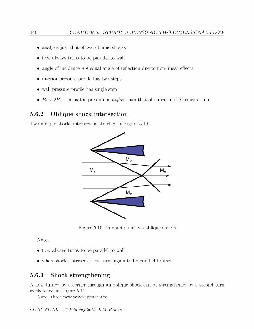
146 CHAPTER 5. STEADY SUPERSONIC TWO-DIMENSIONAL FLOW
• analysis just that of two oblique shocks
• flow always turns to be parallel to wall
• angle of incidence not equal angle of reflection due to non-linear effects
• interior pressure profile has two steps
• wall pressure profile has single step
• P2 > 2P1, that is the pressure is higher than that obtained in the acoustic limit
5.6.2 Oblique shock intersection
Two oblique shocks intersect as sketched in Figure 5.10
Μ1
Μ2
Μ3
Μ2
Figure 5.10: Interaction of two oblique shocks
Note:
• flow always turns to be parallel to wall
• when shocks intersect, flow turns again to be parallel to itself
5.6.3 Shock strengthening
A flow turned by a corner through an oblique shock can be strengthened by a second turnas sketched in Figure 5.11
Note: three new waves generated
CC BY-NC-ND. 17 February 2015, J. M. Powers.

5.7. SUPERSONIC FLOW OVER AIRFOILS 147
slipstream
rarefaction
Figure 5.11: Shock Strengthening Sketch
• strengthened shock
• slipstream in which pressures match, velocity directions match, but velocity magnitudesdiffer
• weak rarefaction wave
5.6.4 Shock weakening
A flow turned by a corner through an oblique shock can be weakened by a second turn assketched in Figure 5.12
Figure 5.12: Shock Weakening Sketch
5.7 Supersonic flow over airfoils
The standard problem in flow over an airfoil is to determine the lift and the drag. While inactual design it is the magnitude of the lift force FL, and drag force FD, that is most crucial,
CC BY-NC-ND. 17 February 2015, J. M. Powers.

148 CHAPTER 5. STEADY SUPERSONIC TWO-DIMENSIONAL FLOW
there exists dimensionless numbers the lift coefficient CL and the drag coefficient CD whichgive good relative measures of airfoil performance.
CL ≡ FL
12ρ1u2
1A(5.194)
CD ≡ FD
12ρ1u2
1A(5.195)
Though this is the traditional formula, it is probably not the best for interpreting how theforces vary when flight speed is varied. This is because when u1, flight speed is varied bothnumerator and denominator change. To remedy this, we can instead scale by the ambientsound speed to define a dimensionless lift force F∗L and dimensionless drag force F∗D:
F∗L ≡ FL
ρ1c21A(5.196)
F∗D ≡ FD
ρ1c21A(5.197)
5.7.1 Flat plate at angle of attack
The simplest problem is that of a flat plate at angle of attack αo. A schematic is illustratedin Figure 5.13. Note:
P2
P2'
P1 T1 M1
αο
far field Mach wave
far field Mach wave
leading edge
rarefaction
leading edge
shock
slipstream
Figure 5.13: Supersonic Flow over a Flat Plate
• flow over the top is turned through an isentropic rarefaction to P2
CC BY-NC-ND. 17 February 2015, J. M. Powers.
5.7. SUPERSONIC FLOW OVER AIRFOILS 149
• flow over the bottom is turned through an oblique shock to P ′2
• Since P ′2 > P2, there is both lift and drag forces!
• both a shock and rarefaction are attached to the trailing edge to turn the flow to thehorizontal
• the flow regions are separated by a slipstream in which pressure and velocity directions
match
• FL = (P ′2 − P2)A cosαo, CL =
(P ′
2−P2) cosαo
1
2ρ1u2
1
• FD = (P ′2 − P2)A sinαo, CD =
(P ′
2−P2) sinαo
1
2ρ1u2
1
• the drag here is known as wave drag or induced drag
• other components of drag, skin friction drag and thickness drag are zero due to inviscidlimit and zero thickness limit
In the small disturbance limit
∆P
P1=
γM21
√
M21 − 1
∆θ (5.198)
P ′2 = P1 +
γP1M21
√
M21 − 1
αo (5.199)
P2 = P1 +γP1M
21
√
M21 − 1
(−αo) (5.200)
P ′2 − P2 =
2γP1M21
√
M21 − 1
αo (5.201)
P ′2 − P2 =
2γP1√
M21 − 1
u21
γP1
ρ1
αo (5.202)
P ′2 − P2 =
2√
M21 − 1
ρ1u21 αo (5.203)
FL =2
√
M21 − 1
ρ1u21 αoA cosαo (5.204)
FL =2
√
M21 − 1
ρ1u21 αoA(1) (5.205)
CL =4αo
√
M21 − 1
(5.206)
CC BY-NC-ND. 17 February 2015, J. M. Powers.

150 CHAPTER 5. STEADY SUPERSONIC TWO-DIMENSIONAL FLOW
FD =2
√
M21 − 1
ρ1u21 αoA sinαo (5.207)
FD =2
√
M21 − 1
ρ1u21 α2
oA (5.208)
CD =4 α2
o√
M21 − 1
(5.209)
F∗L =FL
ρ1c21A=
2 M21αo
√
M21 − 1
(5.210)
F∗D =FD
ρ1c21A=
2 M21α
2o
√
M21 − 1
(5.211)
High Mach number limit: F∗L = 2M1αo (5.212)
High Mach number limit: F∗D = 2M1α2o (5.213)
Dimensionless lift and drag are plotted versus Mach number in Figure 5.14
Example 5.3Lift and Drag on an Inclined Flat Plate
Given: Flat plate, of chord length 2 m, depth 10 m inclined at 20◦ to the horizontal in a freestreamof M1 = 3, P1 = 100 kPa, T1 = 300 K.
Find: Lift and drag forces on the plate.
Analysis: First some preliminaries:
c1 =√
γRT1 =
√
(1.4)
(
287J
kg K
)
(300 K) = 347.2m
s(5.214)
u1 = M1c1 = (3.0)(
347.2m
s
)
= 1, 041.6m
s(5.215)
ρ1 =P1
RT1=
100, 000 Pa(
287 Jkg K
)
(300 K)= 1.1614
kg
m3(5.216)
Po = P1
(
1 +γ − 1
2M2
1
)γ
γ−1
(5.217)
Po = 100 kPa
(
1 +1
532)3.5
= 367.327 kPa (5.218)
In a previous example, we found the oblique shock state under identical conditions:
P ′
2 = 377, 072 Pa (5.219)
Now consider the rarefaction.
CC BY-NC-ND. 17 February 2015, J. M. Powers.

5.7. SUPERSONIC FLOW OVER AIRFOILS 151
0 2 4 6 8 10
0.25
0.5
0.75
1
1.25
1.5
1.75
2
0 2 4 6 8 10
0.1
0.2
0.3
0.4
0.5
F* = F / ρ c A
M 1
1 1 L L
α = 5 ο ο
F* = F / ρ c A 1 1 D D
2
2
Dimensionless Lift Force
Dimensionless Drag Force
α = 5 ο ο
Flat Plate at Small Angle of Attack
Flat Plate at Small Angle of Attack
Invalid Region
Invalid Region
M 1
Figure 5.14: Dimensionless Lift and Drag versus Incoming Mach Number for Flat Plate atSmall Angle of Attack
ν(M1) =
√
γ + 1
γ − 1tan−1
√
γ − 1
γ + 1(M2
1 − 1)− tan−1√
M21 − 1 (5.220)
ν(M1) =
√
1.4 + 1
1.4− 1tan−1
√
1.4− 1
1.4 + 1(32 − 1)− tan−1
√
32 − 1 = 0.8691 rad = 49.7973◦ (5.221)
ν(M2) = ν(M1) + 20◦ (5.222)
ν(M2) = 49.7973◦ + 20◦ = 69.7973◦ (5.223)
69.7973◦ = 1.218 rad =
√
1.4 + 1
1.4− 1tan−1
√
1.4− 1
1.4 + 1(M2
2 − 1)− tan−1√
M22 − 1 (5.224)
M2 = 4.3209 (5.225)
P2 = Po
(
1 +γ − 1
2M2
2
)
−γ
γ−1
(5.226)
P2 = 367.327 kPa
(
1 +1
54.32092
)
−3.5
= 1.591 kPa (5.227)
CC BY-NC-ND. 17 February 2015, J. M. Powers.

152 CHAPTER 5. STEADY SUPERSONIC TWO-DIMENSIONAL FLOW
FL = (P ′
2 − P2)A cosαo (5.228)
FL = (377, 072 Pa− 1, 591 Pa) (10 m) (2 m) cos 20◦ (5.229)
FL = 7, 142, 073 N (5.230)
CL =FL
12ρ1u
21A
=7, 142, 073 N
12
(
1.1614 kgm3
)
(
1, 041.6 ms
)2(10 m) (2 m)
(5.231)
CL = 0.5668 (5.232)
FD = (P ′
2 − P2)A sinαo (5.233)
FD = (377, 072 Pa− 1, 591 Pa) (10 m) (2 m) sin 20◦ (5.234)
FD = 2, 320, 600 N (5.235)
CD =FD
12ρ1u
21A
=2, 320, 600 N
12
(
1.1614 kgm3
)
(
1, 041.6 ms
)2(10 m) (2 m)
(5.236)
CD = 0.1842 (5.237)
Compare with thin airfoil theory: CL thin =4αo
√
M21 − 1
(5.238)
CL thin =4 (20◦) π rad
180◦√32 − 1
= 0.4936 (5.239)
CD thin =4α2
o√
M21 − 1
(5.240)
CD thin =4(
(20◦) π rad180◦
)2
√32 − 1
= 0.1723 (5.241)
5.7.2 Diamond-shaped airfoil
The simplest supersonic airfoil with camber for analysis purposes is the diamond shapedairfoil as sketched in Figure 5.15. The sketch shows the airfoil at zero angle of attack. Theupper half of the wedge is inclined at angle ǫ to the horizontal In this case there will be nolift but there will be drag. Note the following features:
• sudden turn through lead oblique shock
• turn through isentropic Prandtl-Meyer rarefaction
• final turn through oblique shock attached to trailing edge
• far field limit: acoustic (Mach) waves
• Thin airfoil limit CL thin = 4ǫ√M2
1−1
, same as for flat plate!
• Thin airfoil limit CD thin = 4ǫ2√M2
1−1
, same as for flat plate!
CC BY-NC-ND. 17 February 2015, J. M. Powers.

5.7. SUPERSONIC FLOW OVER AIRFOILS 153
2ε
P1 T1 M1
P2 P3 P4
far field Mach waves
lead oblique shock trailing oblique
shock
Prandtl-Meyer rarefaction
Figure 5.15: Supersonic Flow over a Diamond-Shaped Airfoil
5.7.3 General curved airfoil
A general airfoil with camber is sketched in Figure 5.16. The sketch shows the airfoil at zeroangle of attack. In this case there will be no lift but there will be drag. Note the followingfeatures:
• lead oblique shock
• lead shock weakened by series of non-centered rarefaction waves
• shock at trailing edge, also weakened by non-centered rarefaction waves
• far field: acoustic (Mach) waves
5.7.4 Transonic transition
Transonic flow exists whenever there is a continuous transition from subsonic to supersonicflow. One example of a transonic flow is sketched in Figure 5.171 which shows an acceleratingairfoil.
Note:
1adopted from Bryson, A. E., “An Experimental Investigation of Transonic Flow Past Two-DimensionalWedge and Circular-Arc Sections Using a Mach-Zehnder Interferometer,” NACA Tech. Note 2560, 1951.
CC BY-NC-ND. 17 February 2015, J. M. Powers.

154 CHAPTER 5. STEADY SUPERSONIC TWO-DIMENSIONAL FLOW
Figure 5.16: Supersonic Flow over a Curved Airfoil
Μ1 = 0.852 Μ1 = 0.892
Μ1 = 1.207 Μ1 = 1.315 Μ1 = 1.465
Shock
M < 1 M > 1 M < 1
Sonic Locus
Shock
Sonic Locus
M < 1 M > 1 M < 1
Shock
M < 1 M > 1
Sonic Locus
Shock
M < 1 M > 1
Shock
M < 1 M > 1
M > 1
M > 1
Figure 5.17: Transition from Subsonic to Transonic to Supersonic Flow
• for high subsonic Mach number a bubble of supersonic flow appears
• smooth transition from subsonic to supersonic
• shock transition from supersonic to subsonic
• as Mach number increases, supersonic bubble expands
• for slightly supersonic Mach number, new shock approaches from far field
• as supersonic Mach number increases, shock from far field approaches leading edge andsupersonic bubble disappears
• challenging problems, not easily solved till 1960’s!
CC BY-NC-ND. 17 February 2015, J. M. Powers.

Chapter 6
Linear flow analysis
see Anderson, Chapter 9
In this section we consider flows which are
• steady,
• two-dimensional,
• irrotational,
• isentropic,
• calorically perfect, and
• ideal.
The analysis is extensible to other cases.
6.1 Formulation
In lecture a detailed discussion is given in which the linearized velocity potential equation isobtained:
(
1−M2∞) ∂2φ
∂x2+
∂2φ
∂y2= 0. (6.1)
6.2 Subsonic flow
Here we consider flows in which the Mach number is subsonic, but not negligibly small.
155

156 CHAPTER 6. LINEAR FLOW ANALYSIS
6.2.1 Prandtl-Glauret rule
A discussion is given where it is shown that the pressure coefficient on a supersonic airfoilcan be determined in terms of the pressure coefficient known from subsonic theory:
cp =cpo
√
1−M2∞. (6.2)
6.2.2 Flow over wavy wall
The technique of separation of variables is used to show the subsonic flow over a wavy wallcan be written in terms of the velocity potential as
φ(x, y) =U∞h
√
1−M2∞
sin
(
2πx
l
)
exp
(
−2π√
1−M2∞y
l
)
. (6.3)
6.3 Supersonic flow
6.3.1 D’Alembert’s solution
The D’Alembert solution for the wave equation is shown for supersonic flows:
φ(x, y) = f(
x+√
M2∞ − 1y
)
+ g(
x−√
M2∞ − 1y
)
. (6.4)
6.3.2 Flow over wavy wall
The solution for flow over a wavy wall is given in detail in lecture.
CC BY-NC-ND. 17 February 2015, J. M. Powers.

Chapter 7
Viscous flow
This chapter will focus on problems in which viscous stress plays an important role in deter-mining the motion of the fluid. The topic in general is quite broad; to gain understandingof the fundamental physics, we will restrict our attention to the following limits:
• incompressible fluid
• isotropic Newtonian fluid with constant properties
• at most two-dimensional unsteady flow
The chapter will consider the governing equations and then solve a few representativeproblems.
7.1 Governing equations
This section considers the governing equations for the conditions specified for this chapter.In dimensional non-conservative form, the governing equations are as follows:
∂u
∂x+
∂v
∂y= 0
ρ∂u
∂t+ ρu
∂u
∂x+ ρv
∂u
∂y= −∂P
∂x+ µ
(
∂2u
∂x2+
∂2u
∂y2
)
ρ∂v
∂t+ ρu
∂v
∂x+ ρv
∂v
∂y= −∂P
∂y+ µ
(
∂2v
∂x2+
∂2v
∂y2
)
ρcp
(
∂T
∂t+ u
∂T
∂x+ v
∂T
∂y
)
=
(
∂P
∂t+ u
∂P
∂x+ v
∂P
∂y
)
+ k
(
∂2T
∂x2+
∂2T
∂y2
)
+2µ
(
(
∂u
∂x
)2
+1
2
(
∂u
∂y+
∂v
∂x
)2
+
(
∂v
∂y
)2)
157

158 CHAPTER 7. VISCOUS FLOW
An argument could be made to eliminate the viscous dissipation term and the pressurederivatives in the energy equation. The argument is subtle and based on the low Machnumber limit which corresponds to incompressibility.
7.2 Couette flow
Consider a channel flow driven by plate motion See Figure 7.1
x = 0
x
y
y = 0
y = h
U
P 0
T = T
T = T 0
0
P 0
Figure 7.1: Sketch for Couette flow
The mechanics of such a flow can be described by stripping away many extraneous termsfrom the governing equations.
Take
• fully developed velocity and temperature profiles: ∂u∂x
≡ 0, ∂T∂x
≡ 0
• steady flow ∂∂t
≡ 0
• constant pressure field P (x, y, t) = Po
• constant temperature channel walls T (x, 0, t) = T (x, h, t) = To
Since fully developed mass gives:
∂v
∂y= 0 (7.1)
v(x, y) = f(x) (7.2)
and since in order to prevent mass flowing through the wall boundaries, v(x, 0) = v(x, h) = 0,thus
CC BY-NC-ND. 17 February 2015, J. M. Powers.

7.2. COUETTE FLOW 159
v(x, y) = 0 (7.3)
Since ∂u∂x
= 0, ∂u∂t
= 0 and ∂T∂x
= 0, ∂T∂t
= 0, we have at most,
u = u(y) (7.4)
T = T (y) (7.5)
The y momentum equation has no information and x momentum and energy reduce to thefollowing:
0 = µd2u
dy2(7.6)
0 = kd2T
dy2+ µ
(
du
dy
)2
(7.7)
The x momentum equation is thus
d2u
dy2= 0 (7.8)
du
dy= C1 (7.9)
u(y) = C1y + C2 (7.10)
Now applying u(0) = 0 and u(h) = U to fix C1 and C2 we get
u(y) = Uy
h(7.11)
Shear stress:
τyx = µ∂u
∂y(7.12)
τyx = µU
h(7.13)
The energy equation becomes
d2T
dy2= −µ
k
(
du
dy
)2
(7.14)
CC BY-NC-ND. 17 February 2015, J. M. Powers.

160 CHAPTER 7. VISCOUS FLOW
d2T
dy2= −µ
k
U2
h2(7.15)
dT
dy= −µ
k
U2
h2y + C1 (7.16)
T (y) = −1
2
µ
k
U2
h2y2 + C1y + C2 (7.17)
Now T (0) = To and T (h) = To. This fixes the constants, so
T (y) =1
2
µ
kU2
(
(y
h
)
−(y
h
)2)
+ To (7.18)
In dimensionless form this becomes
T − To
To
=1
2
µcpk
U2
cpTo
(
(y
h
)
−(y
h
)2)
(7.19)
T − To
To=
Pr Ec
2
(
(y
h
)
−(y
h
)2)
(7.20)
Prandtl Number: Pr ≡ µcpk
=
µρ
kρcp
=ν
α=
momentum diffusivity
thermal diffusivity(7.21)
Eckert Number: Ec ≡ U2
cpTo=
kinetic energy
thermal energy(7.22)
Now
dT
dy=
1
2
µ
k
U2
h2(h− 2y) (7.23)
qy = −kdT
dy=
1
2µU2
h2(2y − h) (7.24)
qy(0) = −µU2
2h(7.25)
Note:
• at lower wall, heat flux into wall; heat generated in fluid conducted to wall
• wall heat flux magnitude independent of thermal conductivity
• higher plate velocity, higher wall heat flux
• higher viscosity, higher wall heat flux
• thinner gap, higher wall heat flux
CC BY-NC-ND. 17 February 2015, J. M. Powers.

7.3. SUDDENLY ACCELERATED FLAT PLATE 161
Also since Tmax occurs at y = h2
Tmax =1
8
µ
kU2 + To (7.26)
Note:
• high viscosity, high maximum temperature
• high plate velocity, high maximum temperature
• low thermal conductivity, high maximum temperature
Dimensionless wall heat flux given by the Nusselt number:
Nu ≡∣
∣
∣
∣
∣
qy(0)k∆T∆y
∣
∣
∣
∣
∣
=
∣
∣
∣
∣
qy(0)∆y
k∆T
∣
∣
∣
∣
(7.27)
Nu =µU2
2hh2
k 18µkU2
= 2 (7.28)
7.3 Suddenly accelerated flat plate
The problem of pulling a plate suddenly in a fluid which is initially at rest is often knownas Stokes’ First Problem or Rayleigh’s problem.
7.3.1 Formulation
Consider a channel flow driven by a suddenly accelerated plate. See Figure 7.2 Initially,t < 0
• fluid at rest
• plate at rest
For t ≥ 0
• plate pulled at constant velocity U
Assume:
• constant pressure P (x, y, t) = Po
• fully developed flow ∂u∂x
= 0, ∂T∂x
= 0
CC BY-NC-ND. 17 February 2015, J. M. Powers.
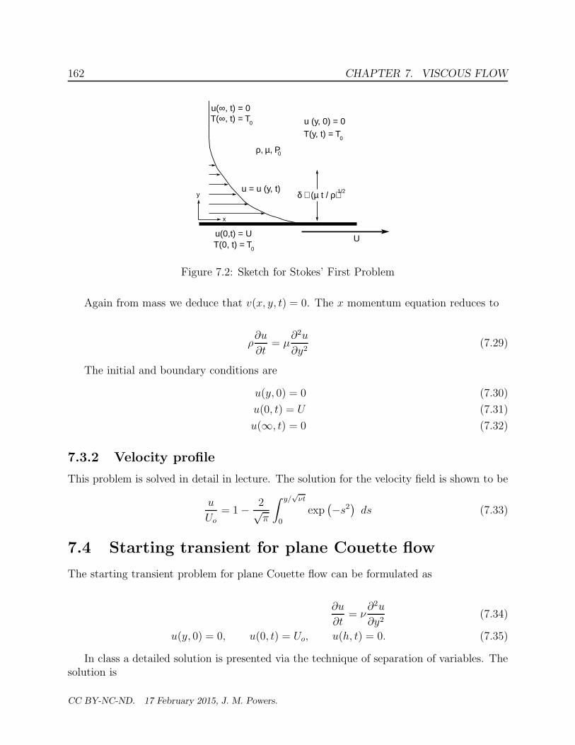
162 CHAPTER 7. VISCOUS FLOW
U
ρ, µ,
u = u (y, t)
u(0,t) = U
u(∞, t) = 0
u (y, 0) = 0
x
y δ ∼ (µ t / ρ) 1/2
P 0
T(∞, t) = T 0
T(y, t) = T 0
T(0, t) = T 0
Figure 7.2: Sketch for Stokes’ First Problem
Again from mass we deduce that v(x, y, t) = 0. The x momentum equation reduces to
ρ∂u
∂t= µ
∂2u
∂y2(7.29)
The initial and boundary conditions are
u(y, 0) = 0 (7.30)
u(0, t) = U (7.31)
u(∞, t) = 0 (7.32)
7.3.2 Velocity profile
This problem is solved in detail in lecture. The solution for the velocity field is shown to be
u
Uo= 1− 2√
π
∫ y/√νt
0
exp(
−s2)
ds (7.33)
7.4 Starting transient for plane Couette flow
The starting transient problem for plane Couette flow can be formulated as
∂u
∂t= ν
∂2u
∂y2(7.34)
u(y, 0) = 0, u(0, t) = Uo, u(h, t) = 0. (7.35)
In class a detailed solution is presented via the technique of separation of variables. Thesolution is
CC BY-NC-ND. 17 February 2015, J. M. Powers.

7.5. BLASIUS BOUNDARY LAYER 163
u
Uo
= 1− y
h− 2
π
∞∑
n=1
1
nexp
(−n2π2νt
h2
)
sin(nπy
h
)
(7.36)
7.5 Blasius boundary layer
The problem of flow over a flat plate in the absence of pressure gradient is formulated andsolved using the classical approach of Blasius.
7.5.1 Formulation
After suitable scaling and definition of similarity variables, discussed in detail in class, thefollowing third order non-linear ordinary differential equation is obtained:
d3f
dη3+
1
2fd2f
dη2= 0, (7.37)
df
dη
∣
∣
∣
∣
η=0
= 0,df
dη
∣
∣
∣
∣
η→∞= 1, f |η=0 = 0. (7.38)
This equation is solved numerically as a homework problem.
7.5.2 Wall shear stress
The solution is used to obtain the classical formulae for skin friction coefficient:
Cf =0.664√Rex
, (7.39)
and drag coefficient:
CD =1.328√ReL
. (7.40)
CC BY-NC-ND. 17 February 2015, J. M. Powers.

164 CHAPTER 7. VISCOUS FLOW
CC BY-NC-ND. 17 February 2015, J. M. Powers.

Chapter 8
Acoustics
This chapter outlines the brief introduction to acoustics given in class in somewhat moredetail.
8.1 Formulation
We reduce the Euler equations for isentropic flow to the following equations where quantitieswith a hat are understood to be small perturbations about the ambient state, denoted witha subscript of ”o”.
∂ρ
∂t+ ρo∇ · v = 0 (8.1)
ρo∂v
∂t+∇ · P = 0 (8.2)
P = c2oρ. (8.3)
Introducing the velocity potential ∇φ = v and employing further manipulation allows theequation to be written as the wave equation:
∂2φ
∂t2= c2o∇2φ. (8.4)
The pressure, velocity, and density are then obtained from
P = −ρo∂φ
∂t, (8.5)
v = ∇φ, (8.6)
ρ = −ρoc2o
∂φ
∂t. (8.7)
165

166 CHAPTER 8. ACOUSTICS
8.2 Planar waves
The D’Alembert solution for planar waves is shown in class to be
φ = f(x+ cot) + g(x− cot), (8.8)
P = −ρocof′(x+ cot) + ρocog
′(x− cot), (8.9)
u = f ′(x+ cot) + g′(x− cot), (8.10)
(8.11)
8.3 Spherical waves
The D’Alembert solution for spherical waves is shown in class to be
φ =1
rf(r + cot) +
1
rg(r − cot), (8.12)
P = −ρocor
f ′(r + cot) +ρocor
g′(r − cot), (8.13)
u =1
rf ′(r + cot) +
1
rg′(r − cot), (8.14)
(8.15)
CC BY-NC-ND. 17 February 2015, J. M. Powers.