Lecture 2 - Silvio Savarese 8-­‐Jan-­‐15  

Professor  Silvio  Savarese  Computa(onal  Vision  and  Geometry  Lab  

Lecture  2  Camera  Models    

Lecture 2 - Silvio Savarese 10-­‐Jan-­‐15  

•   Pinhole  cameras  •   Cameras  &  lenses  •   The  geometry  of  pinhole  cameras  

Lecture  2  Camera  Models    

Reading:    [FP]  Chapter  1,  “Geometric  Camera  Models”      [HZ]  Chapter  6  “Camera  Models”  

Some slides in this lecture are courtesy to Profs. J. Ponce, S. Seitz, F-F Li

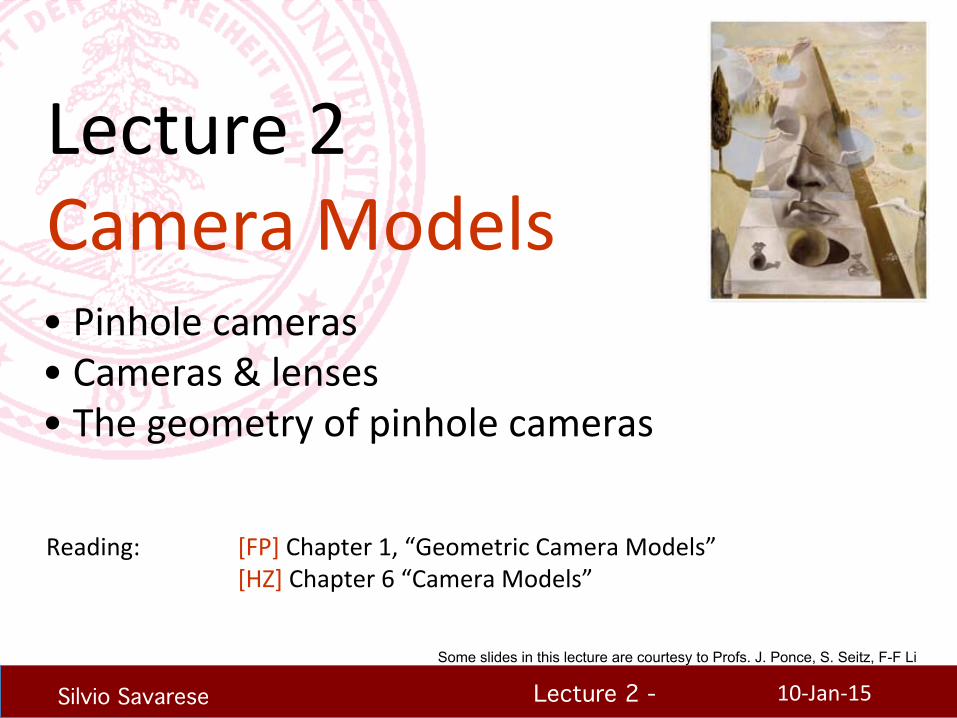
How do we see the world?

•  Let’s design a camera –  Idea 1: put a piece of film in front of an object –  Do we get a reasonable image?

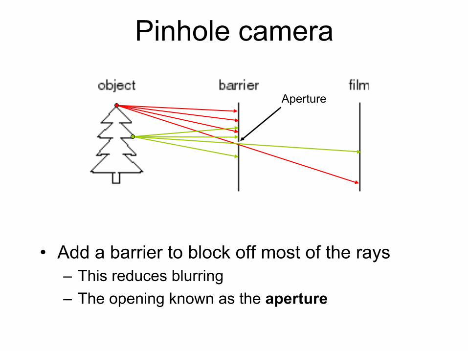
Pinhole camera

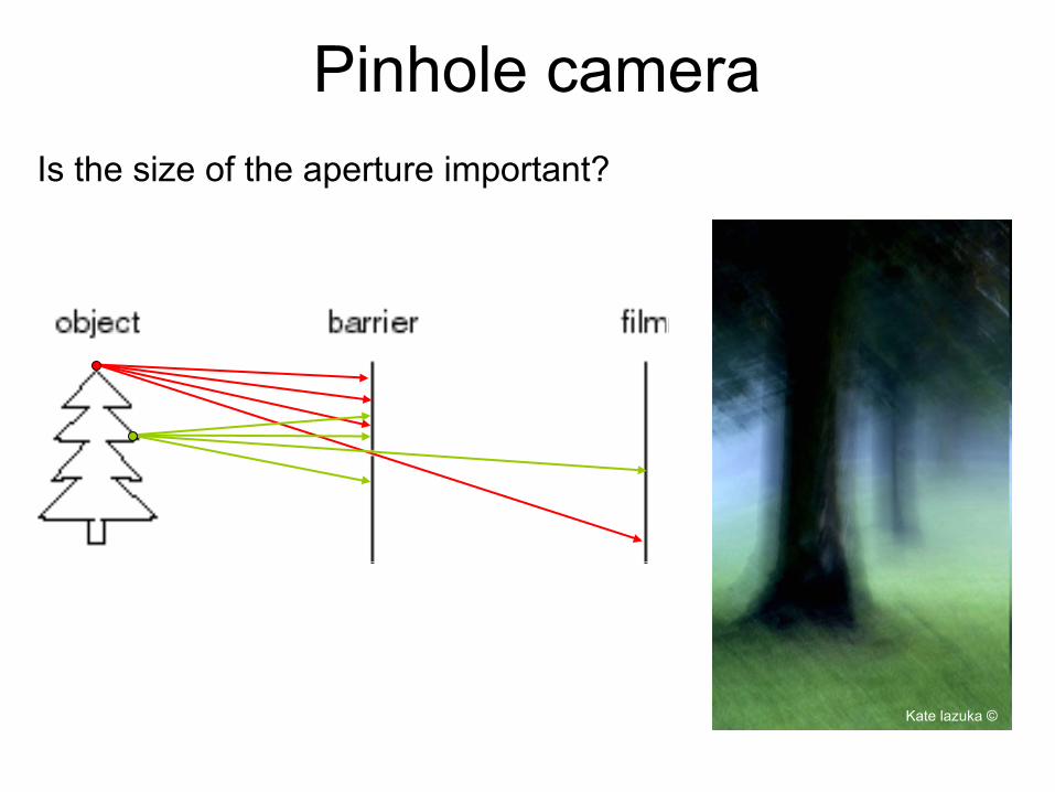
•  Add a barrier to block off most of the rays –  This reduces blurring –  The opening known as the aperture

Aperture

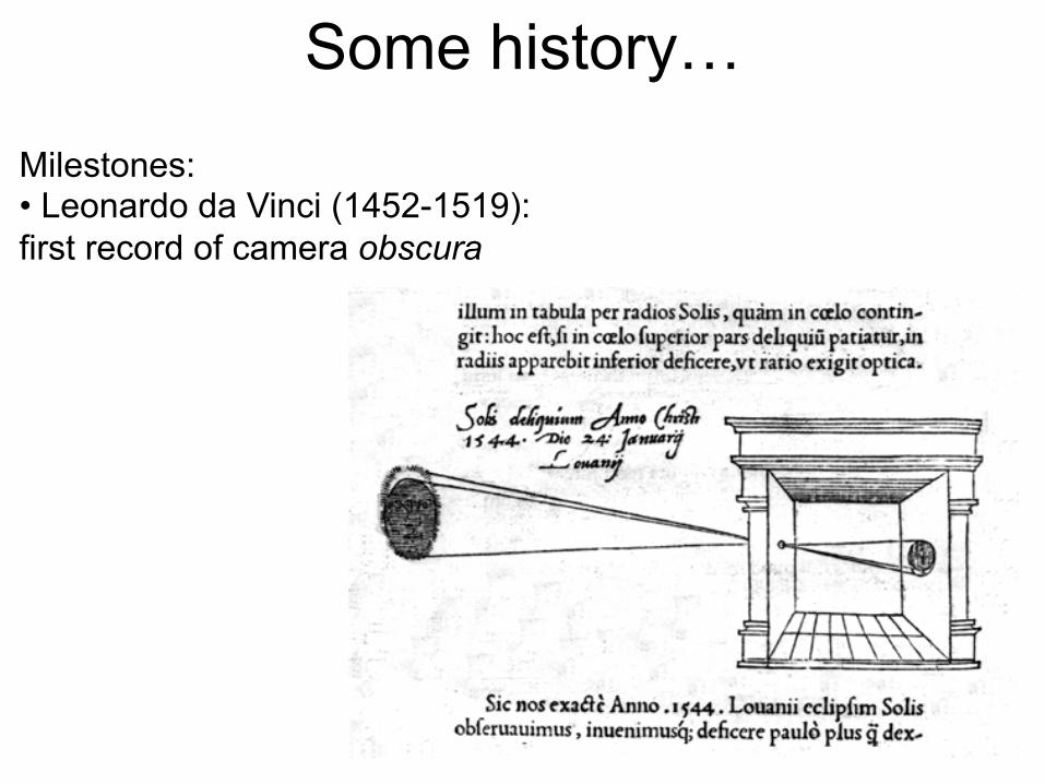
Milestones: •  Leonardo da Vinci (1452-1519): first record of camera obscura

Some history…

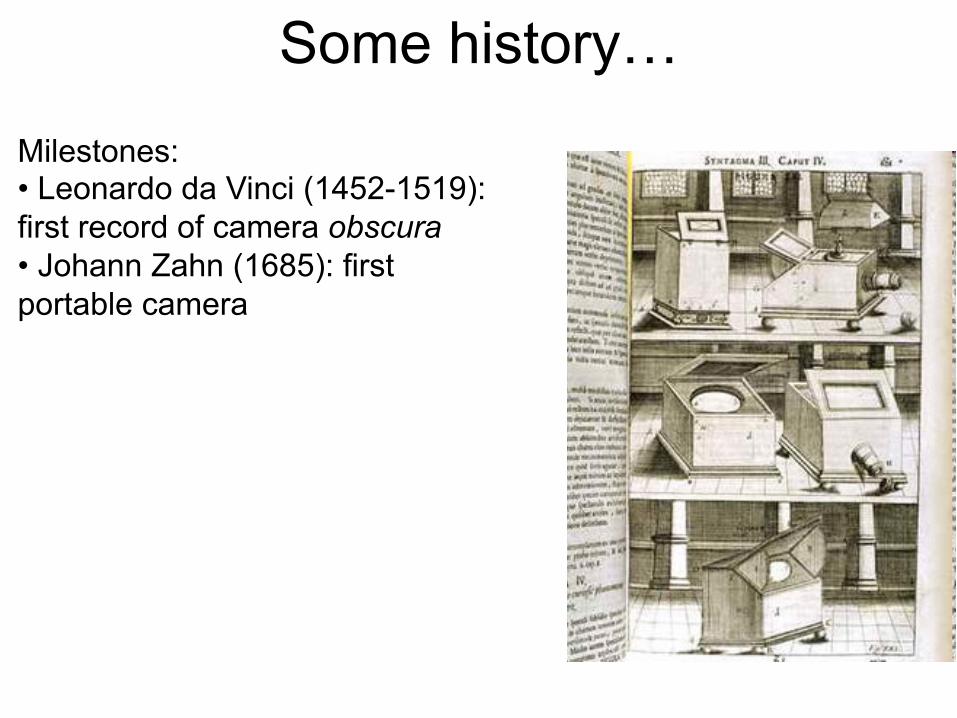
Milestones: •  Leonardo da Vinci (1452-1519): first record of camera obscura •  Johann Zahn (1685): first portable camera

Some history…

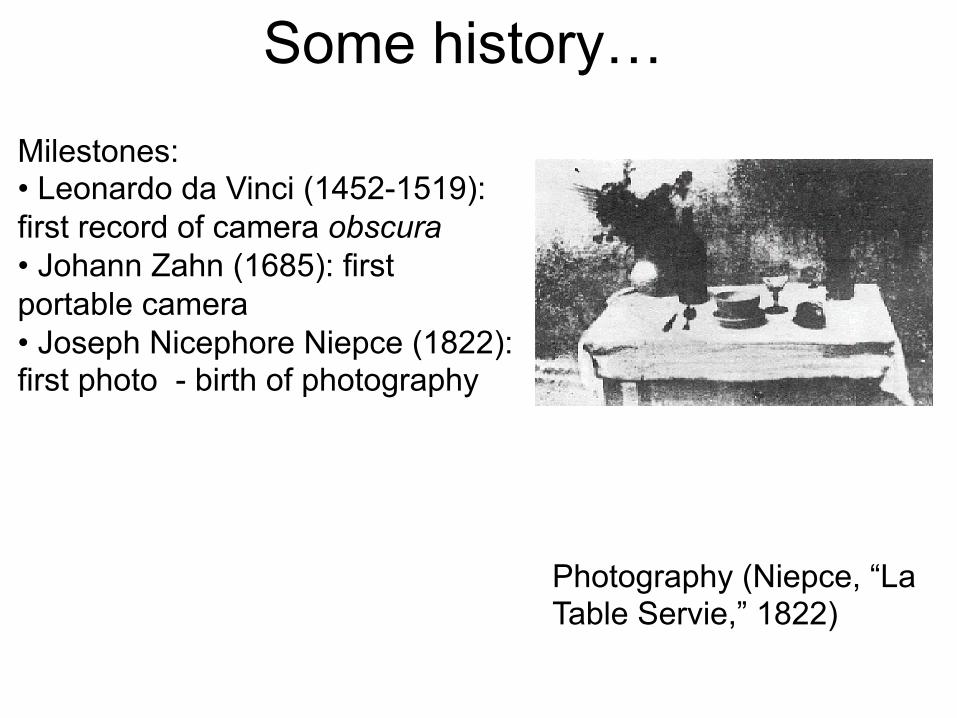
Photography (Niepce, “La Table Servie,” 1822)

Milestones: •  Leonardo da Vinci (1452-1519): first record of camera obscura •  Johann Zahn (1685): first portable camera •  Joseph Nicephore Niepce (1822): first photo - birth of photography

Some history…

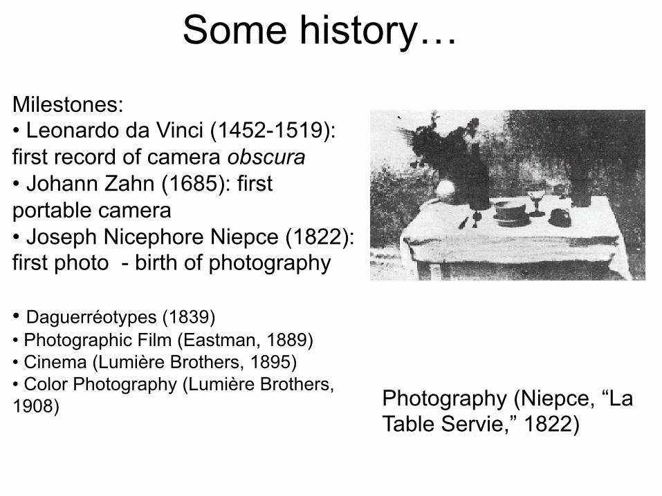
Photography (Niepce, “La Table Servie,” 1822)

Milestones: •  Leonardo da Vinci (1452-1519): first record of camera obscura •  Johann Zahn (1685): first portable camera •  Joseph Nicephore Niepce (1822): first photo - birth of photography

•  Daguerréotypes (1839) •  Photographic Film (Eastman, 1889) •  Cinema (Lumière Brothers, 1895) •  Color Photography (Lumière Brothers, 1908)

Some history…

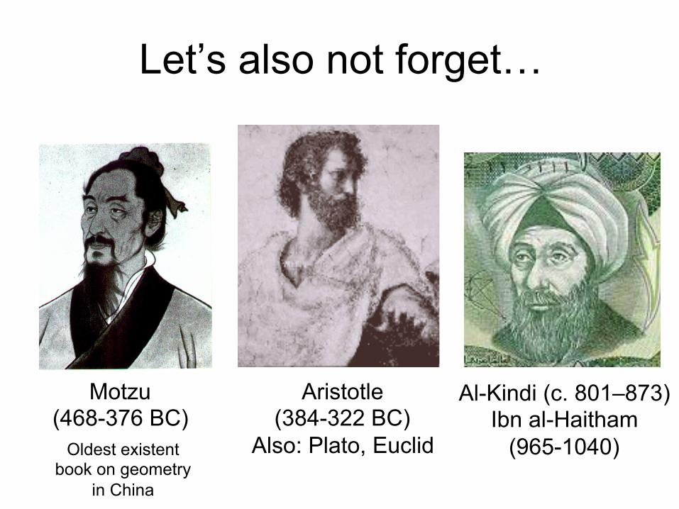
Let’s also not forget…

Motzu (468-376 BC)

Aristotle (384-322 BC)

Also: Plato, Euclid

Al-Kindi (c. 801–873) Ibn al-Haitham

(965-1040) Oldest existent book on geometry

in China

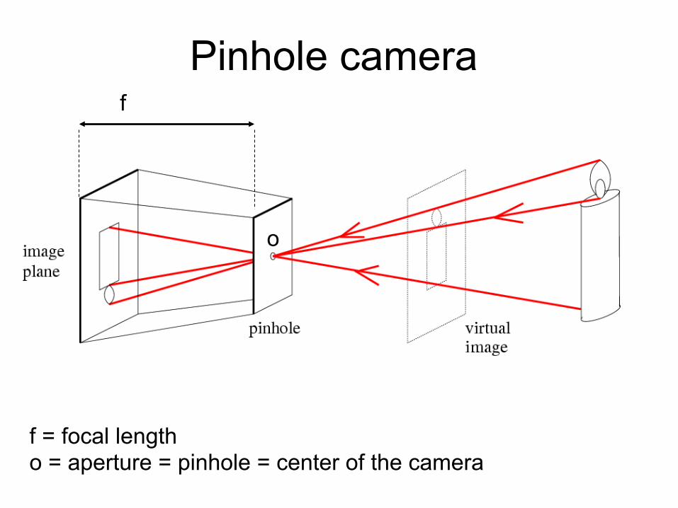
Pinhole perspective projection Pinhole camera f

f = focal length o = aperture = pinhole = center of the camera

o

⎪⎪⎩

⎪⎪⎨

⎧

=

=

zyf'y

zxf'x

⎥⎦

⎤⎢⎣

⎡ʹ′

ʹ′=ʹ′→yx

P⎥⎥⎥

⎦

⎤

⎢⎢⎢

⎣

⎡

=

zyx

P

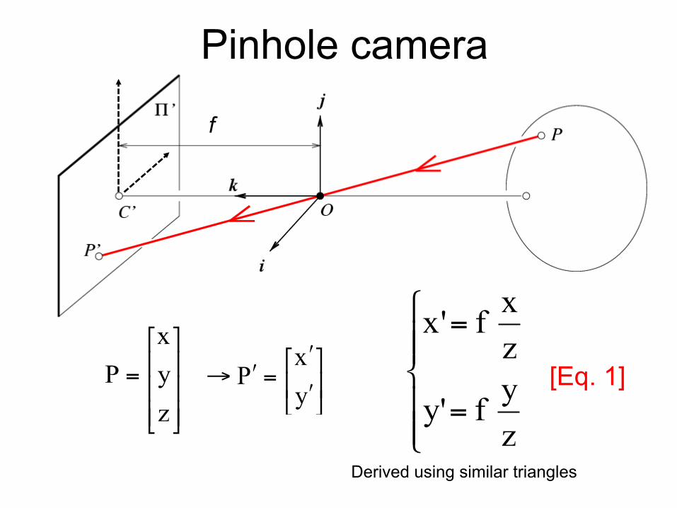
Pinhole camera

Derived using similar triangles

[Eq. 1]

f

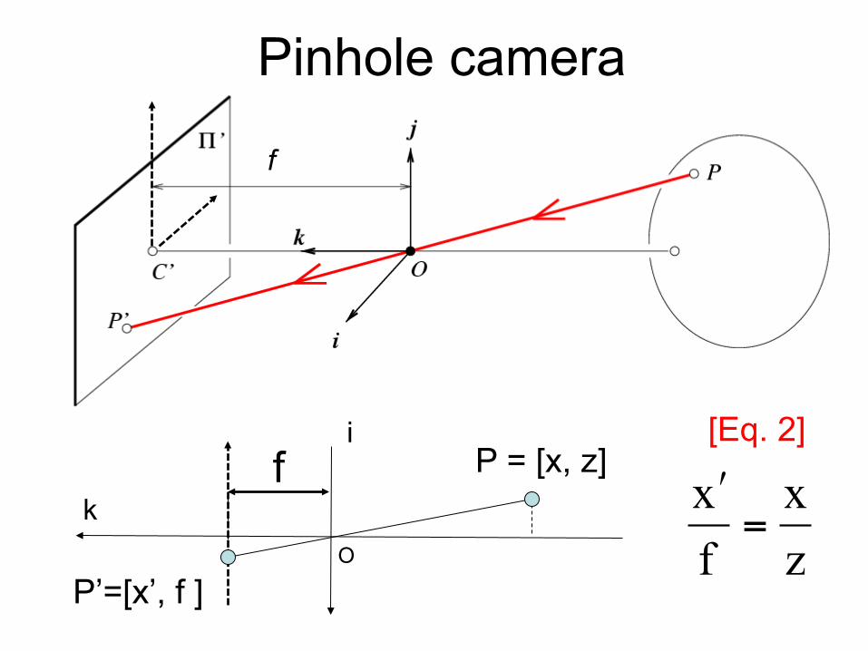
O

P = [x, z]

P’=[x’, f ]

f

zx

fx=ʹ′

i

k

Pinhole camera

[Eq. 2]

f

Kate lazuka ©

Pinhole camera Is the size of the aperture important?

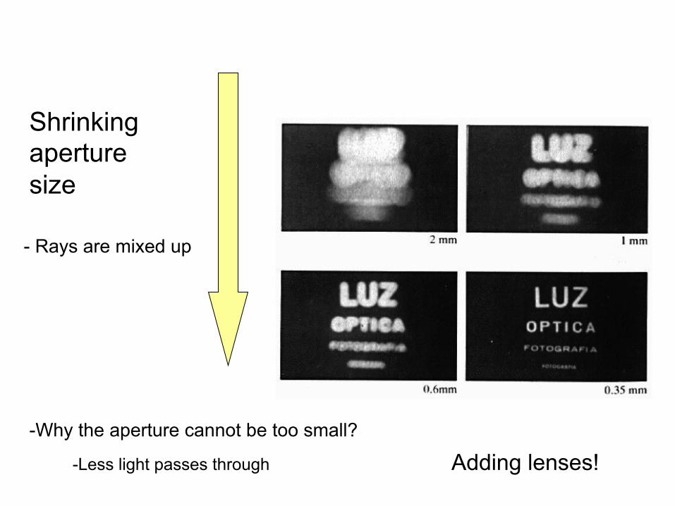
Shrinking aperture size

-  Rays are mixed up

Adding lenses! - Why the aperture cannot be too small?

- Less light passes through

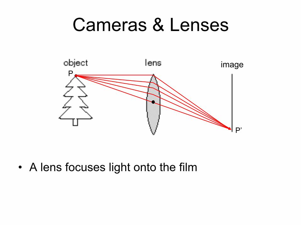
Cameras & Lenses

•  A lens focuses light onto the film

image P

P’

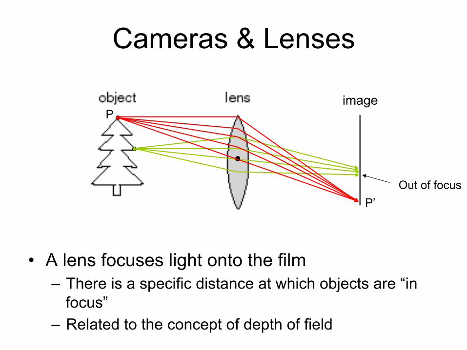
•  A lens focuses light onto the film –  There is a specific distance at which objects are “in

focus” –  Related to the concept of depth of field

Out of focus

Cameras & Lenses

image P

P’

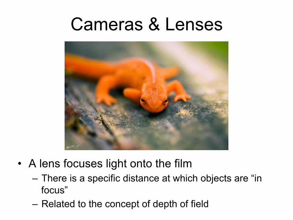
•  A lens focuses light onto the film –  There is a specific distance at which objects are “in

focus” –  Related to the concept of depth of field

Cameras & Lenses

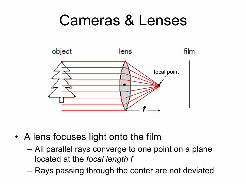
•  A lens focuses light onto the film –  All parallel rays converge to one point on a plane

located at the focal length f –  Rays passing through the center are not deviated

focal point

f

Cameras & Lenses

f

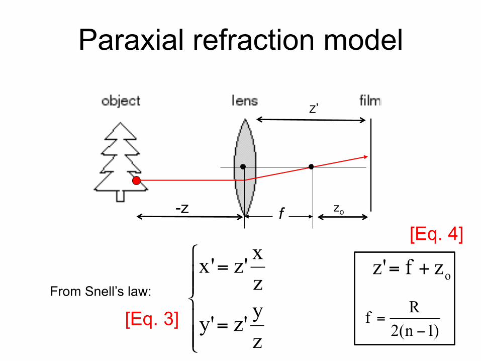
Paraxial refraction model

zy'z'y

zx'z'x

⎪⎪⎩

⎪⎪⎨

⎧

=

= ozf'z +=

)1n(2Rf −

=

zo -z

Z’

From Snell’s law:

[Eq. 3]

[Eq. 4]

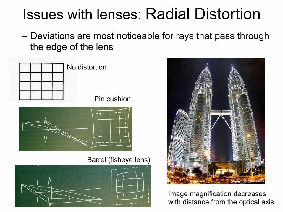
No distortion

Pin cushion

Barrel (fisheye lens)

Issues with lenses: Radial Distortion –  Deviations are most noticeable for rays that pass through

the edge of the lens

Image magnification decreases with distance from the optical axis

Lecture 2 - Silvio Savarese 8-­‐Jan-­‐15  

•   Pinhole  cameras  •   Cameras  &  lenses  •   The  geometry  of  pinhole  cameras  

•  Intrinsic  •  Extrinsic  

Lecture  2  Camera  Models    

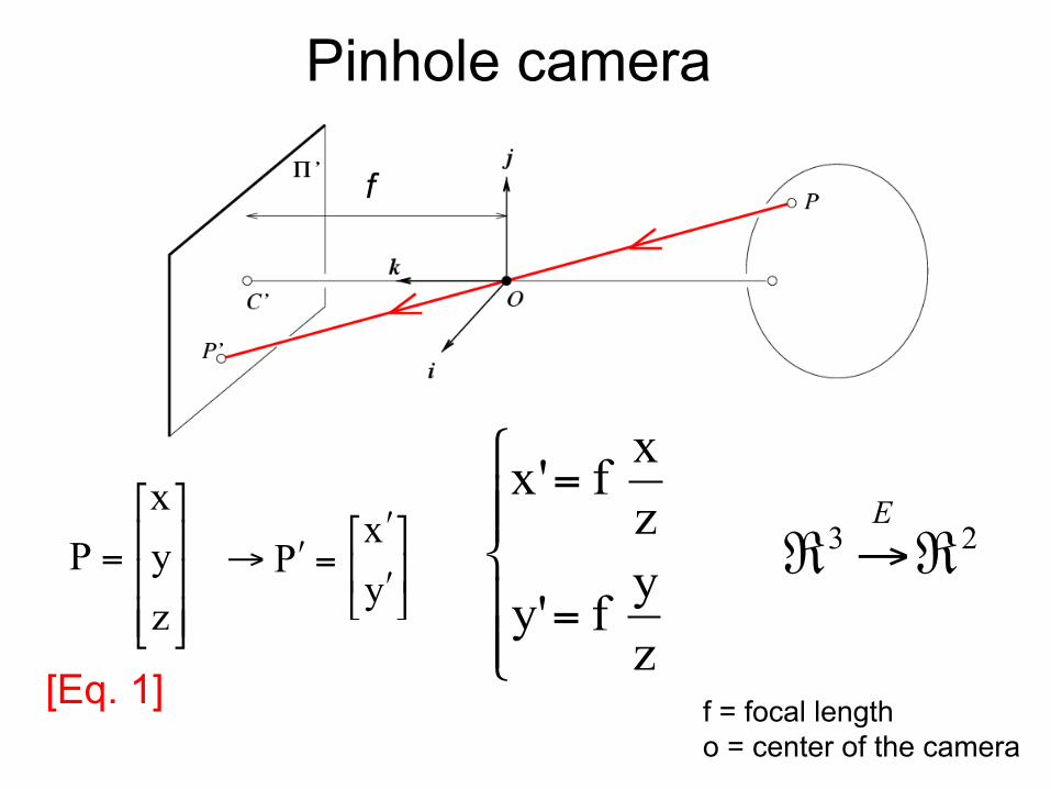
Pinhole perspective projection Pinhole camera

f = focal length o = center of the camera

23 ℜ→ℜE

⎪⎪⎩

⎪⎪⎨

⎧

=

=

zyf'y

zxf'x

⎥⎦

⎤⎢⎣

⎡ʹ′

ʹ′=ʹ′→yx

P⎥⎥⎥

⎦

⎤

⎢⎢⎢

⎣

⎡

=

zyx

P

[Eq. 1]

f

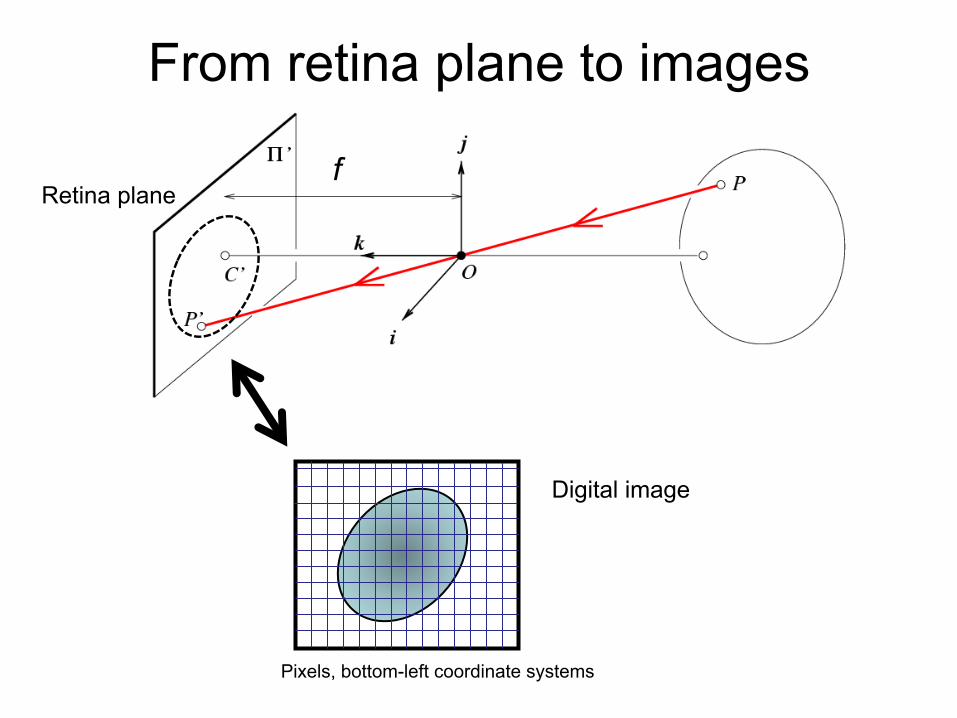
From retina plane to images

Pixels, bottom-left coordinate systems

f Retina plane

Digital image

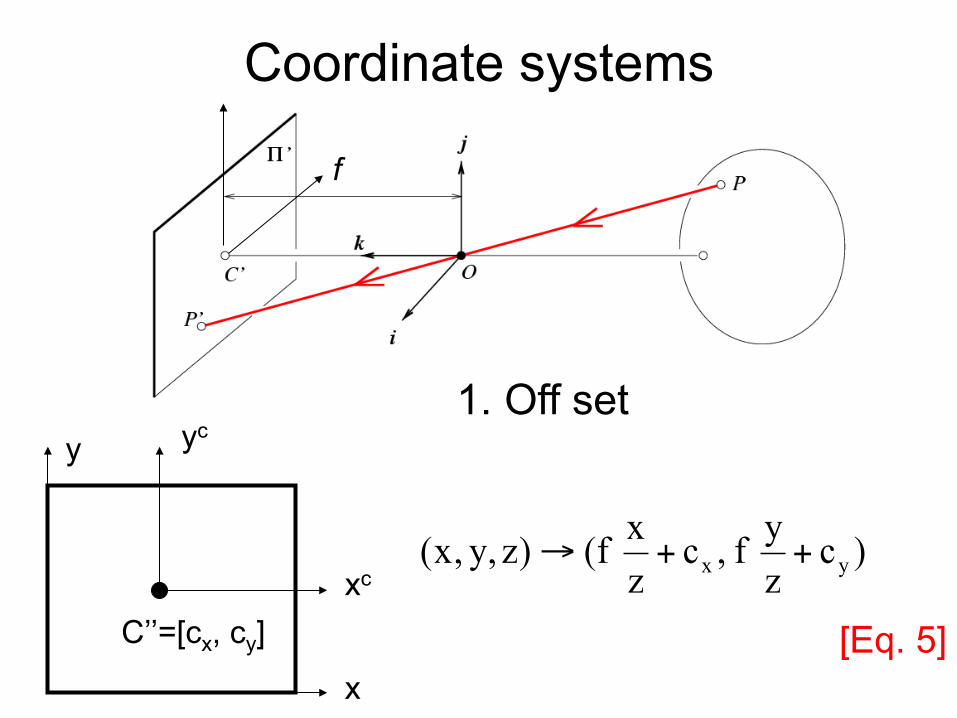
Coordinate systems

f

x

y

xc

yc

C’’=[cx, cy]

)czyf,c

zxf()z,y,x( yx ++→

1. Off set

[Eq. 5]

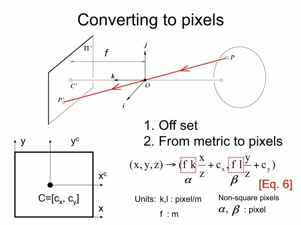
Converting to pixels

)czylf,c

zxkf()z,y,x( yx ++→

1. Off set 2. From metric to pixels

x

y

xc

yc

C=[cx, cy] Units: k,l : pixel/m

f : m : pixel

α β

,α βNon-square pixels

f

[Eq. 6]

•  Is this a linear transformation?

x

y

xc

yc

C=[cx, cy]

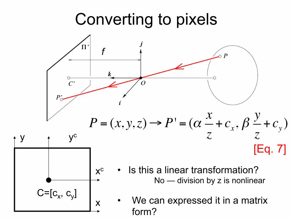
P = (x, y, z)→ P ' = (α xz+ cx, β

yz+ cy )

Converting to pixels

f

[Eq. 7]

No — division by z is nonlinear

•  We can expressed it in a matrix form?

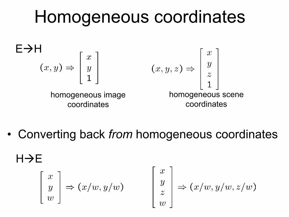
Homogeneous coordinates

homogeneous image coordinates

homogeneous scene coordinates

•  Converting back from homogeneous coordinates

EàH

HàE

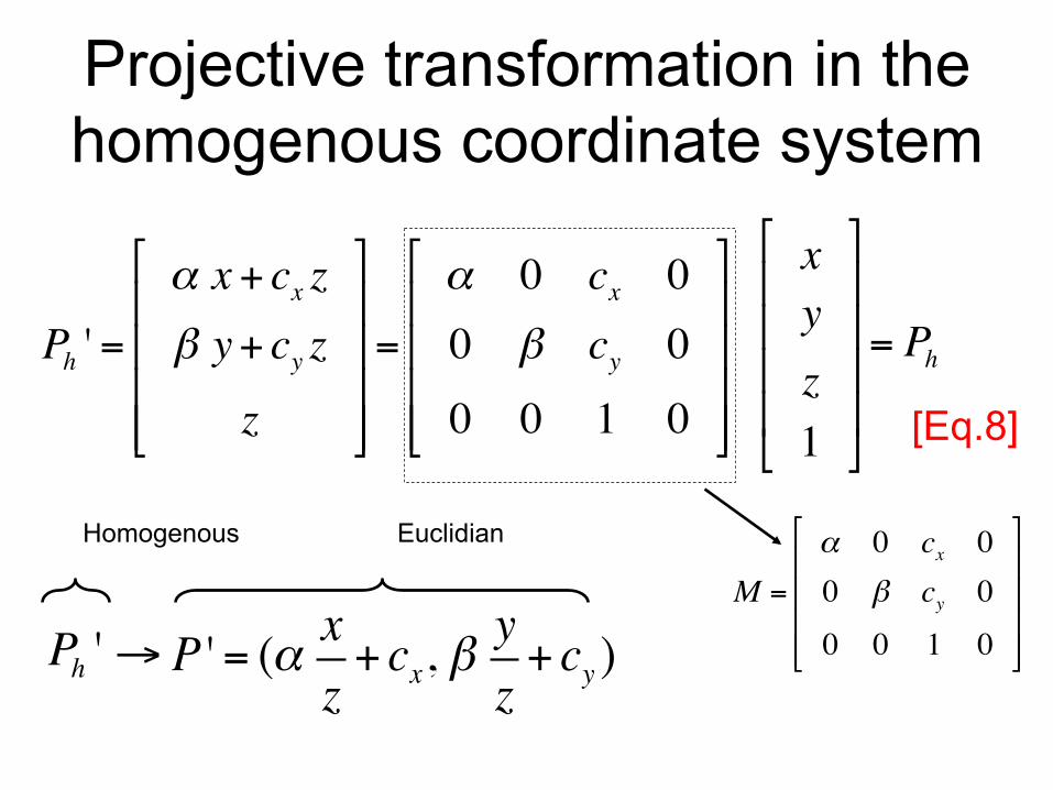
Projective transformation in the homogenous coordinate system

xyz1

!

"

####

$

%

&&&&

= Ph

M =

α 0 cx 00 β cy 0

0 0 1 0

!

"

####

$

%

&&&&

[Eq.8]

→ P ' = (α xz+ cx, β

yz+ cy )Ph '

Homogenous Euclidian

Ph ' =α x + cx zβ y+ cy z

z

!

"

####

$

%

&&&&

=

α 0 cx 00 β cy 0

0 0 1 0

!

"

####

$

%

&&&&

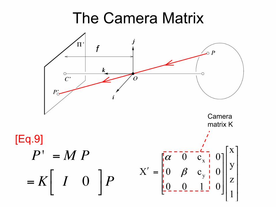
P ' =M P

= K I 0!"

#$P

The Camera Matrix

⎥⎥⎥⎥

⎦

⎤

⎢⎢⎢⎢

⎣

⎡

⎥⎥⎥

⎦

⎤

⎢⎢⎢

⎣

⎡

=ʹ′

1zyx

01000c00c0

X y

x

β

α

Camera matrix K

f

[Eq.9]

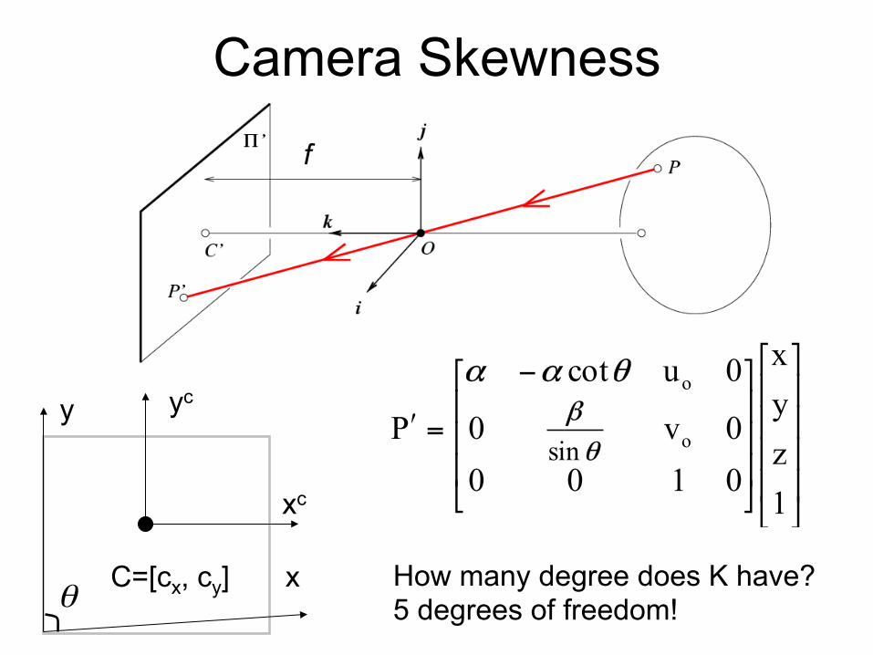
Camera Skewness

x

y

xc

yc

C=[cx, cy] θHow many degree does K have? 5 degrees of freedom!

f

⎥⎥⎥⎥

⎦

⎤

⎢⎢⎢⎢

⎣

⎡

⎥⎥⎥

⎦

⎤

⎢⎢⎢

⎣

⎡ −

=ʹ′

1zyx

01000v0

0ucot

P o

o

sinθβ

θαα

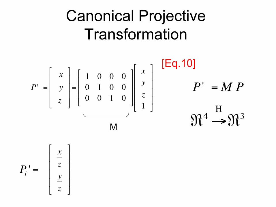
Canonical Projective Transformation

P ' =xyz

!

"

####

$

%

&&&&

=1 0 0 00 1 0 00 0 1 0

!

"

###

$

%

&&&

xyz1

!

"

####

$

%

&&&&

xzyz

!

"

####

$

%

&&&&

Pi ' =

P ' =M P

M 3

H4 ℜ→ℜ

[Eq.10]

Lecture 2 - Silvio Savarese 8-­‐Jan-­‐15  

•   Pinhole  cameras  •   Cameras  &  lenses  •   The  geometry  of  pinhole  cameras  

•  Intrinsic  •  Extrinsic  

•   Other  camera  models  

Lecture  2  Camera  Models    

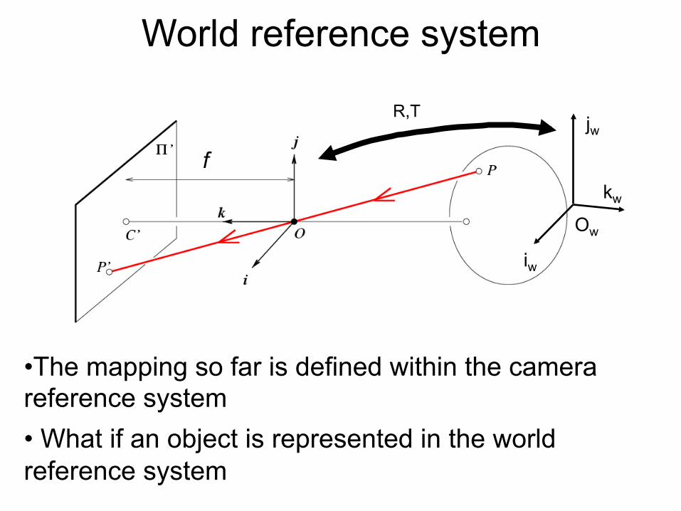
World reference system

Ow

iw

kw

jw R,T

• The mapping so far is defined within the camera reference system •  What if an object is represented in the world reference system

f

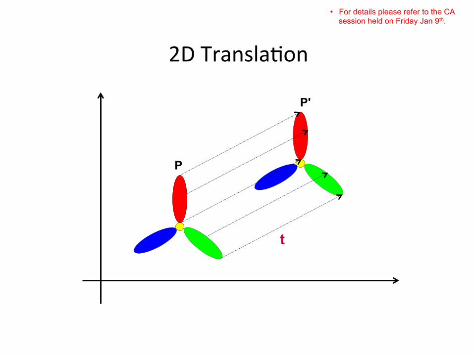
2D  TranslaUon  

P

P'

t

•  For details please refer to the CA session held on Friday Jan 9th.

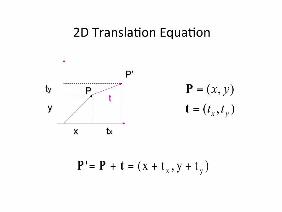
2D  TranslaUon  EquaUon  

P

x

y

tx

ty

P’

t

)ty,tx(' yx ++=+= tPP

),(),(

yx ttyx

=

=

tP

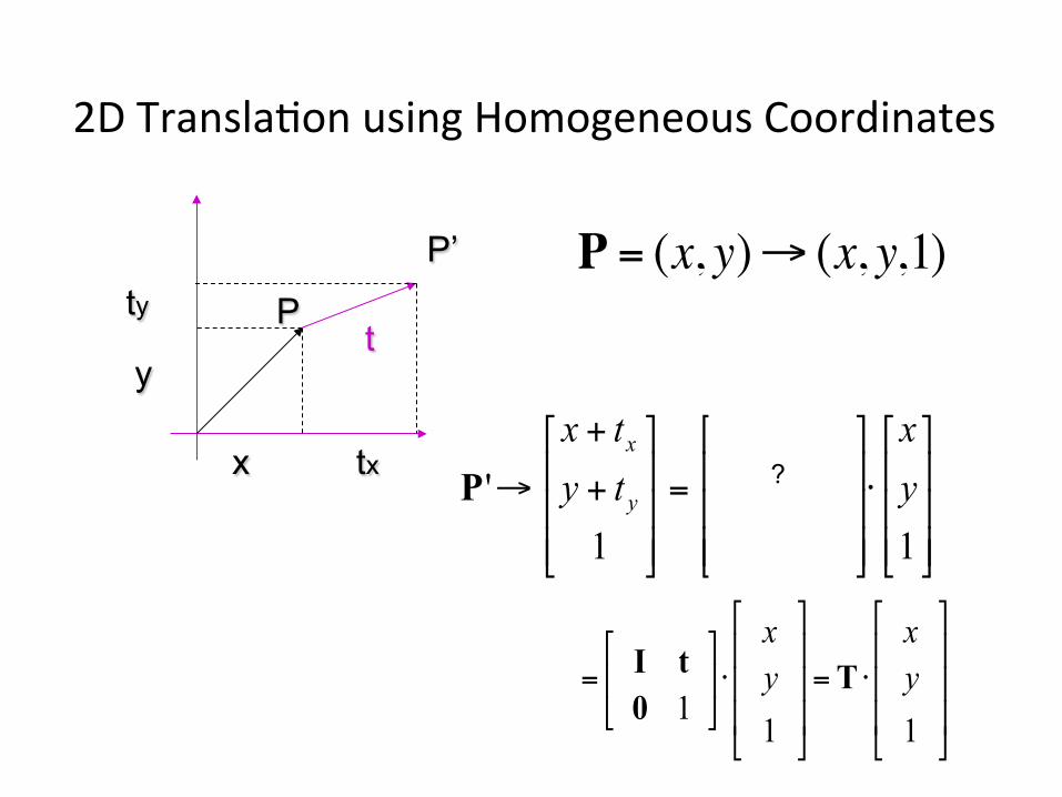
2D  TranslaUon  using  Homogeneous  Coordinates  

⎥⎥⎥

⎦

⎤

⎢⎢⎢

⎣

⎡

⋅

⎥⎥⎥

⎦

⎤

⎢⎢⎢

⎣

⎡

=

⎥⎥⎥

⎦

⎤

⎢⎢⎢

⎣

⎡

+

+

→

11001001

1' y

xtt

tytx

y

x

y

x

P

P = (x, y)→ (x, y,1)

= I t0 1

!

"#

$

%&⋅

xy1

!

"

###

$

%

&&&=T ⋅

xy1

!

"

###

$

%

&&&

P

x

y

tx

ty

P’

t

?

Scaling  

P

P'

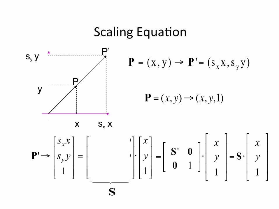
Scaling  EquaUon  

P

x

y

sx x

P’ sy y

⎥⎥⎥

⎦

⎤

⎢⎢⎢

⎣

⎡

⋅

⎥⎥⎥

⎦

⎤

⎢⎢⎢

⎣

⎡

=

⎥⎥⎥

⎦

⎤

⎢⎢⎢

⎣

⎡

→

11000000

1' y

xs

sysxs

y

x

y

x

P

P = (x, y)→ (x, y,1)

S

= S ' 00 1

!

"#

$

%&⋅

xy1

!

"

###

$

%

&&&= S ⋅

xy1

!

"

###

$

%

&&&

)ys,xs(')y,x( yx=→= PP

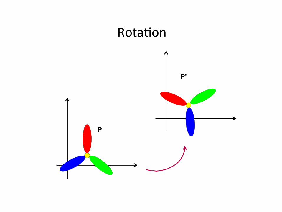
RotaUon  

P

P'

RotaUon  EquaUons  •  Counter-­‐clockwise  rotaUon  by  an  angle  𝜃  

⎥⎦

⎤⎢⎣

⎡⎥⎦

⎤⎢⎣

⎡ −=⎥

⎦

⎤⎢⎣

⎡

yx

yx

θθ

θθ

cossinsincos

''P

x

y’ P’

θ

x’ y PRP' =

' cos sinx x yθ θ= −

' cos siny y xθ θ= +

How  many  degrees  of  freedom?     1   P '→cosθ −sinθ 0sinθ cosθ 00 0 1

#

$

%%%

&

'

(((

xy1

#

$

%%%

&

'

(((

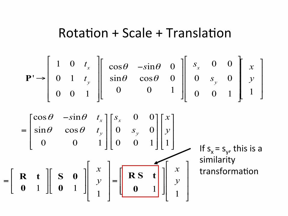
RotaUon  +  Scale  +  TranslaUon  

P '→

1 0 tx0 1 ty0 0 1

"

#

$$$$

%

&

''''

cosθ −sinθ 0sinθ cosθ 00 0 1

"

#

$$$

%

&

'''

sx 0 0

0 sy 0

0 0 1

"

#

$$$$

%

&

''''

xy1

"

#

$$$

%

&

'''

cos in 0 0sin cos 0 00 0 1 0 0 1 1

x x

y y

s t s xt s y

θ θθ θ

−⎡ ⎤ ⎡ ⎤ ⎡ ⎤⎢ ⎥ ⎢ ⎥ ⎢ ⎥= ⎢ ⎥ ⎢ ⎥ ⎢ ⎥⎢ ⎥ ⎢ ⎥ ⎢ ⎥⎣ ⎦ ⎣ ⎦ ⎣ ⎦

= R t0 1

!

"#

$

%& S 00 1

!

"#

$

%&xy1

!

"

###

$

%

&&&= R S t

0 1

!

"##

$

%&&

xy1

!

"

###

$

%

&&&

If  sx  =  sy,  this  is  a  similarity    transformaUon  

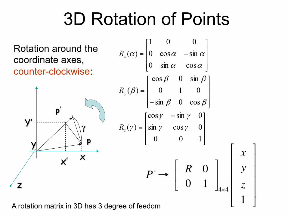
3D Rotation of Points Rotation around the coordinate axes, counter-clockwise:

⎥⎥⎥

⎦

⎤

⎢⎢⎢

⎣

⎡ −

=

⎥⎥⎥

⎦

⎤

⎢⎢⎢

⎣

⎡

−

=

⎥⎥⎥

⎦

⎤

⎢⎢⎢

⎣

⎡

−=

1000cossin0sincos

)(

cos0sin010

sin0cos)(

cossin0sincos0001

)(

γγ

γγ

γ

ββ

ββ

β

αα

ααα

z

y

x

R

R

R

p

x

Y’ p’

γ

x’

y

z P '→ R 0

0 1

"

#$

%

&'4×4

xyz1

"

#

$$$$

%

&

''''

A rotation matrix in 3D has 3 degree of feedom

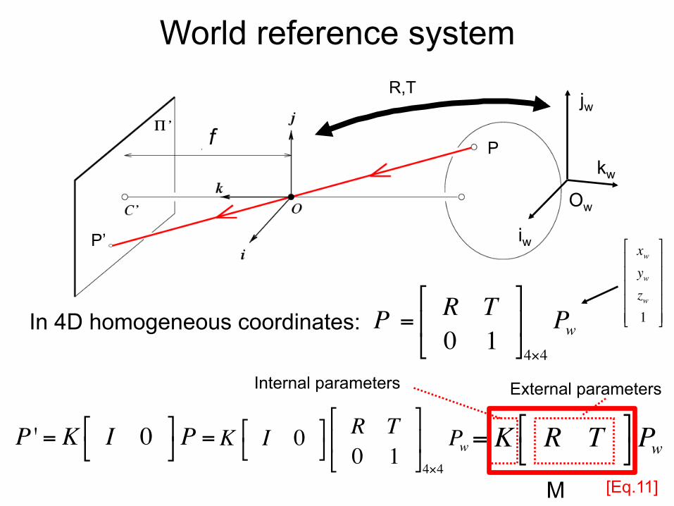
= K R T!"

#$Pw

World reference system

Ow

iw

kw

jw R,T

P = R T0 1

!

"#

$

%&4×4

PwIn 4D homogeneous coordinates:

Internal parameters External parameters

P ' = K I 0!"

#$P =K I 0!

"#$

R T0 1

!

"%

#

$&4×4

Pw

M

P

P’

f

xwywzw1

!

"

#####

$

%

&&&&&

[Eq.11]

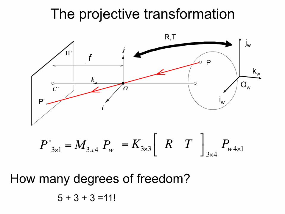
P '3×1 =M3x4 Pw = K3×3 R T"#

$% 3×4

Pw4×1

The projective transformation

Ow

iw

kw

jw R,T

How many degrees of freedom? 5 + 3 + 3 =11!

P

P’

f

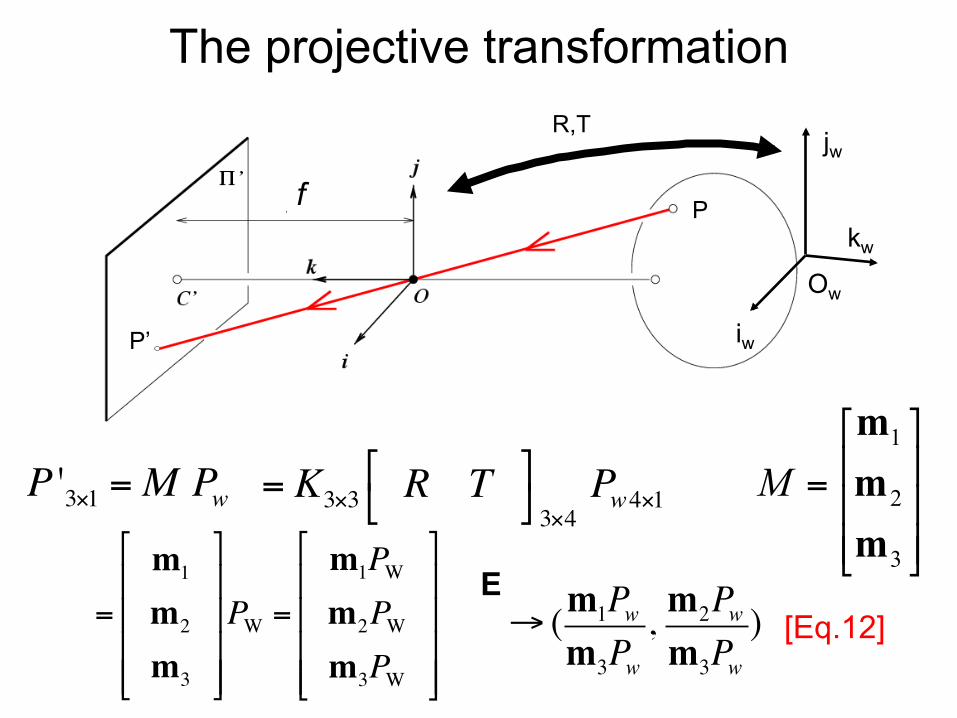
The projective transformation

Ow

iw

kw

jw R,T

P '3×1 =M Pw = K3×3 R T"#

$% 3×4

Pw4×1⎥⎥⎥

⎦

⎤

⎢⎢⎢

⎣

⎡

=

3

2

1

mmm

M

=

m1

m2

m3

!

"

####

$

%

&&&&

PW =m1PWm2PWm3PW

!

"

####

$

%

&&&&

→ (m1Pwm3Pw

, m2Pwm3Pw

)E

P

P’

f

[Eq.12]

Theorem (Faugeras, 1993)

⎥⎥⎥

⎦

⎤

⎢⎢⎢

⎣

⎡

=

3

2

1

aaa

A[ ] [ ] ][ bATKRKTRKM ===[Eq.13]

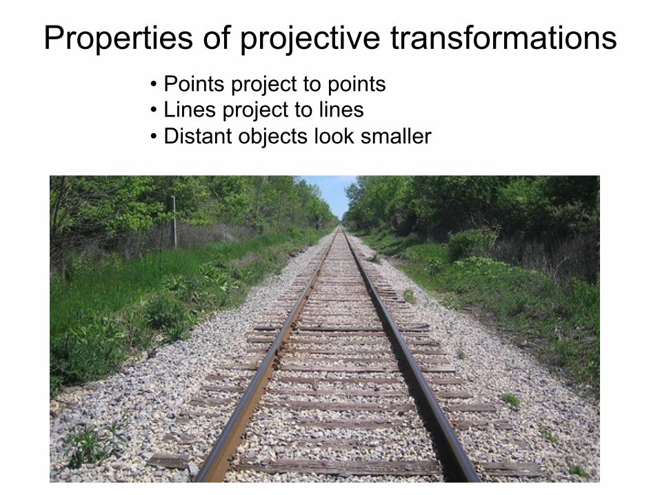
Properties of projective transformations •  Points project to points •  Lines project to lines •  Distant objects look smaller

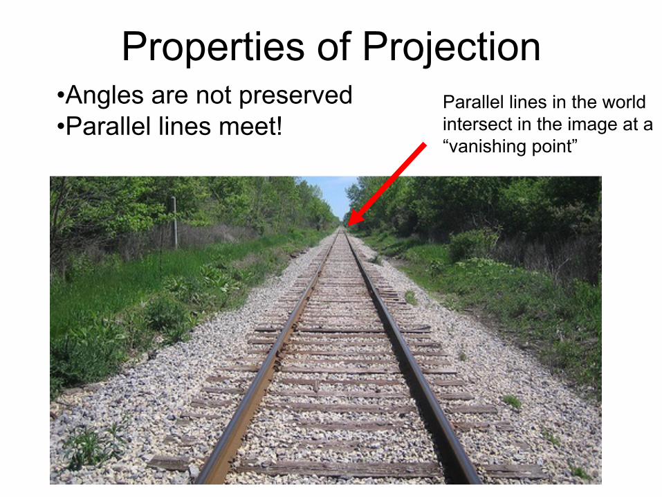
Properties of Projection

• Angles are not preserved • Parallel lines meet!

Parallel lines in the world intersect in the image at a “vanishing point”

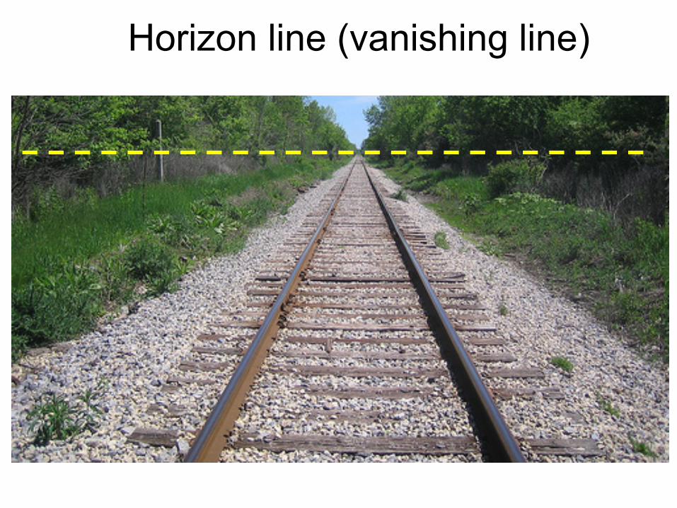
Horizon line (vanishing line)

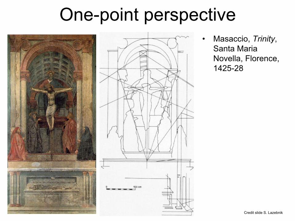
One-point perspective •  Masaccio, Trinity,

Santa Maria Novella, Florence, 1425-28

Credit slide S. Lazebnik

Next lecture

• How to calibrate a camera?

Supplemental material

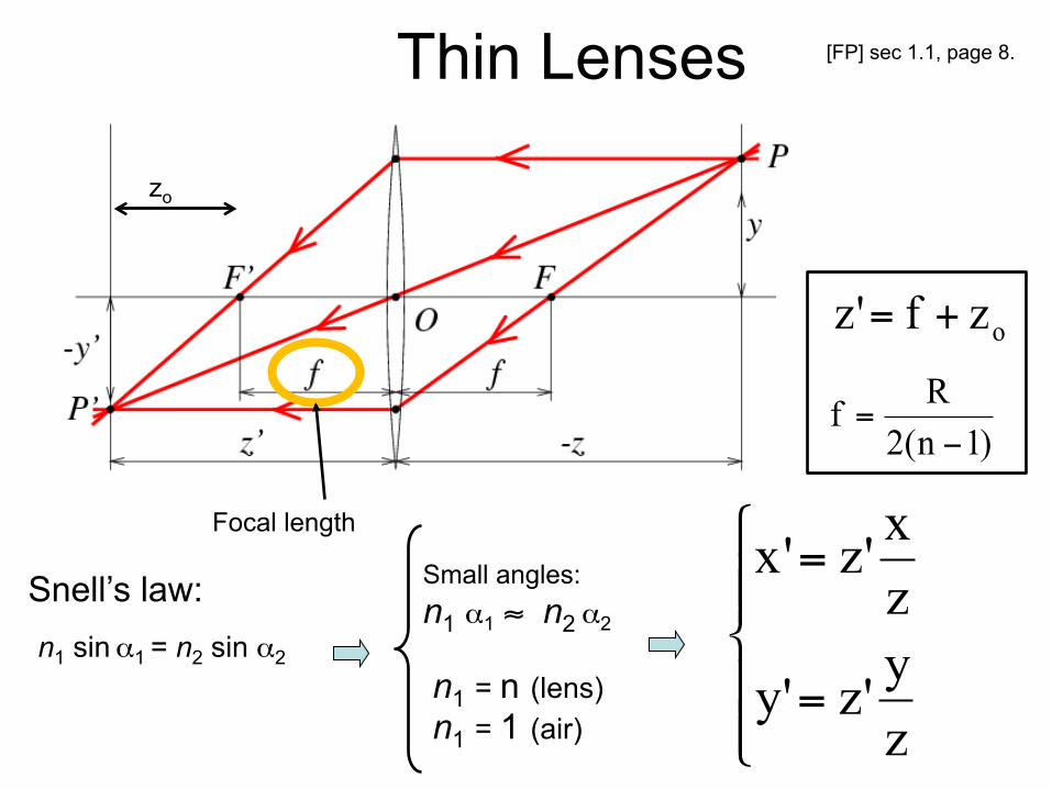
Thin Lenses

Snell’s law:

n1 sin α1 = n2 sin α2

Small angles: n1 α1 ≈ n2 α2

n1 = n (lens) n1 = 1 (air)

zo

zy'z'y

zx'z'x

⎪⎪⎩

⎪⎪⎨

⎧

=

=

ozf'z +=

)1n(2Rf −

=

Focal length

[FP] sec 1.1, page 8.

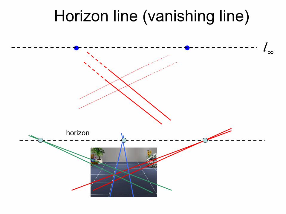
Horizon line (vanishing line)

horizon

∞l