Embed Size (px)
Citation preview

NPTEL- Probability and Distributions
Dept. of Mathematics and Statistics Indian Institute of Technology, Kanpur 1
MODULE 3
FUNCTION OF A RANDOM VARIABLE AND ITS
DISTRIBUTION
LECTURES 12-16
Topics
3.1 FUNCTION OF A RANDOM VARIABLE
3.2 PROBABILITY DISTRIBUTION OF A FUNCTION OF
A RANDOM VARIABLE
3.3 EXPECTATION AND MOMENTS OF A RANDOM
VARIABLE
3.4 PROPERTIES OF RANDOM VARIABLES HAVING
THE SAME DISTRIBUTION
3.5 PROBABILITY AND MOMENT INEQUALITIES 3.5.1 Markov Inequality 3.5.2 Chebyshev Inequality
3.5.3 Jensen Inequality 3.5.4 𝑨𝑴-𝑮𝑴-𝑯𝑴 inequality
3.6 DESCRIPTIVE MEASURES OF PROBABILITY
DISTRIBUTIONS 3.6.1 Measures of Central Tendency
3.6.1.1 Mean 3.6.1.2 Median 3.6.1.3 Mode
3.6.2 Measures of Dispersion
3.6.2.1 Standard Deviation 3.6.2.2 Mean Deviation 3.6.2.3 Quartile Deviation 3.6.2.4 Coefficient of Variation

NPTEL- Probability and Distributions
Dept. of Mathematics and Statistics Indian Institute of Technology, Kanpur 2
3.7 MEASURES OF SKEWNESS
3.8 MEASURES OF KURTOSIS
MODULE 3
FUNCTION OF A RANDOM VARIABLE AND ITS
DISTRIBUTION
LECTURE 12
Topics
3.1 FUNCTION OF A RANDOM VARIABLE
3.2 PROBABILITY DISTRIBUTION OF A FUNCTION OF
A RANDOM VARIABLE
3.1 FUNCTION OF A RANDOM VARIABLE
Let 𝛺,ℱ,𝑃 be a probability space and let 𝑋 be random variable defined on 𝛺,ℱ,𝑃 .
Further let ℎ:ℝ → ℝ be a given function and let 𝑍:𝛺 → ℝbe a function of random
variable 𝑋, defined by 𝑍 𝜔 = ℎ 𝑋 𝜔 ,𝜔 ∈ 𝛺. In many situations it may be of interest
to study the probabilistic properties of 𝑍, which is a function of random variable 𝑋. Since
the variable 𝑍 takes values in ℝ, to study the probabilistic properties of 𝑍, it is necessary
that 𝑍−1 𝐵 ∈ ℱ,∀𝐵 ∈ ℬ1, i.e., 𝑍 is a random variable. Throughout, for a positive integer
𝑘,ℝ𝑘 will denote the 𝑘-dimensional Euclidean space and ℬ𝑘 will denote the Borel sigma-
field in ℝ𝑘 .
Definition 1.1 Let 𝑘 and 𝑚 be positive integers. A function ℎ:ℝ𝑘 → ℝ𝑚 is said to be a Borel function if
ℎ−1 𝐵 ∈ ℬ𝑘 ,∀𝐵 ∈ ℬ𝑚 . ▄
NPTEL- Probability and Distributions
Dept. of Mathematics and Statistics Indian Institute of Technology, Kanpur 3
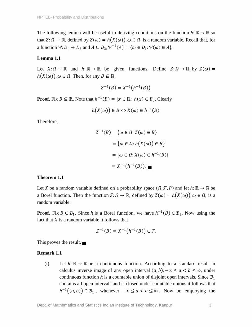
The following lemma will be useful in deriving conditions on the function ℎ:ℝ → ℝ so
that 𝑍:𝛺 → ℝ, defined by 𝑍 𝜔 = ℎ 𝑋 𝜔 ,𝜔 ∈ 𝛺, is a random variable. Recall that, for
a function Ψ:𝐷1 → 𝐷2 and 𝐴 ⊆ 𝐷2, Ψ−1 𝐴 = 𝜔 ∈ 𝐷1: Ψ 𝜔 ∈ 𝐴 .
Lemma 1.1
Let 𝑋:𝛺 → ℝ and ℎ:ℝ → ℝ be given functions. Define 𝑍:𝛺 → ℝ by 𝑍 𝜔 =
ℎ 𝑋 𝜔 ,𝜔 ∈ 𝛺. Then, for any 𝐵 ⊆ ℝ,
𝑍−1 𝐵 = 𝑋−1 ℎ−1 𝐵 .
Proof. Fix 𝐵 ⊆ ℝ. Note that ℎ−1 𝐵 = 𝑥 ∈ ℝ: ℎ 𝑥 ∈ 𝐵 . Clearly
ℎ 𝑋 𝜔 ∈ 𝐵 ⇔ 𝑋 𝜔 ∈ ℎ−1 𝐵 .
Therefore,
𝑍−1 𝐵 = 𝜔 ∈ 𝛺: 𝑍 𝜔 ∈ 𝐵
= 𝜔 ∈ 𝛺: ℎ 𝑋 𝜔 ∈ 𝐵
= 𝜔 ∈ 𝛺: 𝑋 𝜔 ∈ ℎ−1 𝐵
= 𝑋−1 ℎ−1 𝐵 . ▄
Theorem 1.1
Let 𝑋 be a random variable defined on a probability space 𝛺,ℱ,𝑃 and let ℎ:ℝ → ℝ be
a Borel function. Then the function 𝑍:𝛺 → ℝ, defined by 𝑍 𝜔 = ℎ 𝑋 𝜔 ,𝜔 ∈ 𝛺, is a
random variable.
Proof. Fix 𝐵 ∈ ℬ1. Since ℎ is a Borel function, we have ℎ−1 𝐵 ∈ ℬ1. Now using the
fact that 𝑋 is a random variable it follows that
𝑍−1 𝐵 = 𝑋−1 ℎ−1 𝐵 ∈ ℱ.
This proves the result. ▄
Remark 1.1
(i) Let ℎ:ℝ → ℝ be a continuous function. According to a standard result in
calculus inverse image of any open interval 𝑎, 𝑏 ,−∞ ≤ 𝑎 < 𝑏 ≤ ∞, under
continuous function ℎ is a countable union of disjoint open intervals. Since ℬ1
contains all open intervals and is closed under countable unions it follows that
ℎ−1 𝑎, 𝑏 ∈ ℬ1 , whenever −∞ ≤ 𝑎 < 𝑏 ≤ ∞ . Now on employing the

NPTEL- Probability and Distributions
Dept. of Mathematics and Statistics Indian Institute of Technology, Kanpur 4
arguments similar to the one used in proving Theorem 1.1, Module 2 (also see
Theorem 1.2, Module 2) we conclude that ℎ−1 𝐵 ∈ ℬ1,∀𝐵 ∈ ℬ1. It follows
that any continuous function ℎ:ℝ → ℝ is a Borel function and thus, in view of
Theorem 1.1, any continuous function of a random variable is a random
variable. In particular if 𝑋 is a random variable then 𝑋2 , 𝑋 , max 𝑋, 0 , sin𝑋
and cos𝑋 are random variables.
(ii) Let ℎ:ℝ → ℝ be a strictly monotone function. Then, for −∞ ≤ 𝑎 < 𝑏 ≤ ∞,
ℎ−1 𝑎, 𝑏 is a countable union of intervals and therefore ℎ−1 𝑎, 𝑏 ∈ ℬ1, i.e.,
ℎ is a Borel function. It follows that if 𝑋 is a random variable and if ℎ:ℝ → ℝ
is strictly monotone then ℎ(𝑋) is a random variable. ▄
A random variable 𝑋 takes values in various Borel sets according to some probability law
called the probability distribution of random variable 𝑋 . Clearly the probability
distribution of a random variable of absolutely continuous/discrete type is described by
its distribution function (d.f.) and/or by its probability density function/probability mass
function (p.d.f/p.m.f.). For a given Borel function ℎ:ℝ → ℝ, in the following section, we
will derive probability distribution of ℎ(𝑋) using the probability distribution of random
variable 𝑋. ▄
3.2 PROBABILITY DISTRIBUTION OF A FUNCTION OF A
RANDOM VARIABLE
In our future discussions when we refer to a random variable, unless otherwise stated, it
will be either of discrete type or of absolutely continuous type. The probability
distribution of a discrete type random variable will be referred to as a discrete
(probability) distribution and the probability distribution of a random variable of
absolutely continuous type will be referred to as an absolutely continuous (probability)
distribution.
The following theorem deals with discrete probability distributions.
Theorem 2.1 Let 𝑋 be a random variable of discrete type with support 𝑆𝑋 and p.m.f. 𝑓𝑋(⋅) . Let
ℎ:ℝ → ℝ be a Borel function and let 𝑍:𝛺 → ℝ be defined by 𝑍 𝜔 = ℎ 𝑋 𝜔 ,𝜔 ∈ Ω.
Then 𝑍 is a random variable of discrete type with support 𝑆𝑍 = ℎ 𝑥 :𝑥 ∈ 𝑆𝑋 and p.m.f.

NPTEL- Probability and Distributions
Dept. of Mathematics and Statistics Indian Institute of Technology, Kanpur 5
𝑓𝑍 𝑧 = 𝑓𝑋 𝑥 , if 𝑧 ∈ 𝑆𝑍𝑥∈𝐴𝑧
0, otherwise
= 𝑃 𝑋 ∈ 𝐴𝑧 , if 𝑧 ∈ 𝑆𝑍0, otherwise
,
where 𝐴𝑧 = 𝑥 ∈ 𝑆𝑋 : ℎ 𝑥 = 𝑧 . Proof. Since ℎ is a Borel function, using Theorem 1.1, it follows that 𝑍 is a random
variable. Also 𝑋 is of discrete implies that 𝑆𝑋 is countable which further implies that 𝑆𝑍
is countable. Fix 𝑧0 ∈ 𝑆𝑍, so that 𝑧0 = ℎ 𝑥0 for some 𝑥0 ∈ 𝑆𝑋 .
Then
𝑋 = 𝑥0 = 𝜔 ∈ 𝛺:𝑋 𝜔 = 𝑥0 ⊆ 𝜔 ∈ 𝛺: ℎ 𝑋 𝜔 = ℎ 𝑥0
= ℎ 𝑋 = ℎ 𝑥0
= 𝑍 = 𝑧0 ,
and
𝑋 ∈ 𝑆𝑋 = 𝜔 ∈ 𝛺: 𝑋 𝜔 ∈ 𝑆𝑋 ⊆ 𝜔 ∈ 𝛺: ℎ 𝑋 𝜔 ∈ 𝑆𝑍
= ℎ 𝑋 ∈ 𝑆𝑍
= 𝑍 ∈ 𝑆𝑍 .
Therefore,
𝑃 𝑍 = 𝑧0 ≥ 𝑃 𝑋 ∈ 𝑥0 > 0, (since 𝑥0 ∈ 𝑆𝑋),
and 𝑃 𝑍 ∈ 𝑆𝑍 ≥ 𝑃 𝑋 ∈ 𝑆𝑋 = 1.
It follows that 𝑆𝑍 is countable, 𝑃 𝑍 = 𝑧 > 0,∀𝑧 ∈ 𝑆𝑍 and 𝑃 𝑍 ∈ 𝑆𝑍 = 1, i. e., 𝑍 is
a discrete type random variable with support 𝑆𝑍.
Moreover, for 𝑧 ∈ 𝑆𝑍,
𝑃 𝑍 = 𝑧 = 𝑃 𝜔 ∈ 𝛺:ℎ 𝑋 𝜔 = 𝑧
= 𝑃 𝑋 = 𝑥
𝑥∈𝐴𝑧
= 𝑓𝑋 𝑥
𝑥∈𝐴𝑧
= 𝑃 𝑋 ∈ 𝐴𝑧 .
Hence the result follows. ▄
The following corollary is an immediate consequence of the above theorem.
NPTEL- Probability and Distributions
Dept. of Mathematics and Statistics Indian Institute of Technology, Kanpur 6
Corollary 2.1
Under the notation and assumptions of Theorem 2.1, suppose that ℎ:ℝ → ℝ is one-one
with inverse function ℎ−1:𝐷 → ℝ, where 𝐷 = ℎ 𝑥 : 𝑥 ∈ ℝ . Then 𝑍 is a discrete type
random variable with support 𝑆𝑧 = ℎ 𝑥 :𝑥 ∈ 𝑆𝑋 and p.m.f.
𝑓𝑍 𝑧 = 𝑓𝑋 ℎ
−1 𝑧 , if 𝑧 ∈ 𝑆𝑍0, otherwise
= 𝑃 𝑋 = ℎ−1 𝑧 , if 𝑧 ∈ 𝑆𝑍0, otherwise
. ▄
Example 2.1
Let 𝑋 be a random variable with p.m.f.
𝑓𝑋 𝑥 =
1
7, if 𝑥 ∈ −2,−1, 0, 1
3
14, if 𝑥 ∈ 2, 3
0, otherwise
.
Show that 𝑍 = 𝑋2 is a random variable. Find its p.m.f. and distribution function.
Solution. Since ℎ 𝑥 = 𝑥2, 𝑥 ∈ ℝ, is a continuous function and 𝑋 is a random variable,
using Remark 1.1 (i) it follows that 𝑍 = ℎ 𝑋 = 𝑋2 is a random variable. Clearly
𝑆𝑋 = −2,−1, 0, 1, 2, 3 and 𝑆𝑍 = 0, 1, 4, 9 . Moreover,
𝑃 𝑍 = 0 = 𝑃 𝑋2 = 0 = 𝑃 𝑋 = 0 =1
7,
𝑃 𝑍 = 1 = 𝑃 𝑋2 = 1 = 𝑃 𝑋 ∈ −1, 1 =1
7+
1
7=
2
7,
𝑃 𝑍 = 4 = 𝑃 𝑋2 = 4 = 𝑃 𝑋 ∈ −2, 2 =1
7+
3
14=
5
14,
and 𝑃 𝑍 = 9 = 𝑃 𝑋2 = 9 = 𝑃 𝑋 ∈ −3, 3 = 0 +3
14=
3
14∙
Therefore the p.m.f. of 𝑍 is
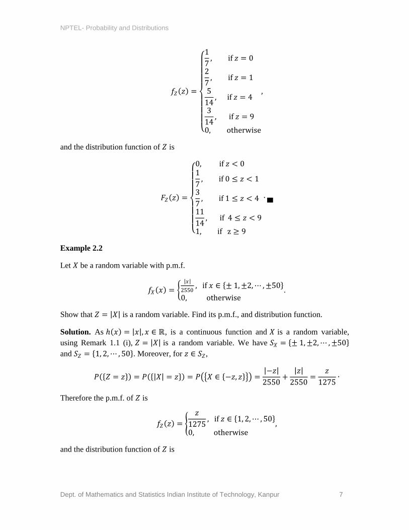
NPTEL- Probability and Distributions
Dept. of Mathematics and Statistics Indian Institute of Technology, Kanpur 7
𝑓𝑍 𝑧 =
1
7, if 𝑧 = 0
2
7, if 𝑧 = 1
5
14, if 𝑧 = 4
3
14, if 𝑧 = 9
0, otherwise
,
and the distribution function of 𝑍 is
𝐹𝑍 𝑧 =
0, if 𝑧 < 01
7, if 0 ≤ 𝑧 < 1
3
7, if 1 ≤ 𝑧 < 4
11
14, if 4 ≤ 𝑧 < 9
1, if z ≥ 9
∙ ▄
Example 2.2
Let 𝑋 be a random variable with p.m.f.
𝑓𝑋 𝑥 = 𝑥
2550, if 𝑥 ∈ ± 1, ±2,⋯ , ±50
0, otherwise
.
Show that 𝑍 = 𝑋 is a random variable. Find its p.m.f., and distribution function.
Solution. As ℎ 𝑥 = 𝑥 ,𝑥 ∈ ℝ, is a continuous function and 𝑋 is a random variable,
using Remark 1.1 (i), 𝑍 = 𝑋 is a random variable. We have 𝑆𝑋 = ± 1, ±2,⋯ , ±50
and 𝑆𝑍 = 1, 2,⋯ , 50 . Moreover, for 𝑧 ∈ 𝑆𝑍,
𝑃 𝑍 = 𝑧 = 𝑃 𝑋 = 𝑧 = 𝑃 𝑋 ∈ −𝑧, 𝑧 = −𝑧
2550+
𝑧
2550=
𝑧
1275∙
Therefore the p.m.f. of 𝑍 is
𝑓𝑍 𝑧 =
𝑧
1275, if 𝑧 ∈ 1, 2,⋯ , 50
0, otherwise,
and the distribution function of 𝑍 is
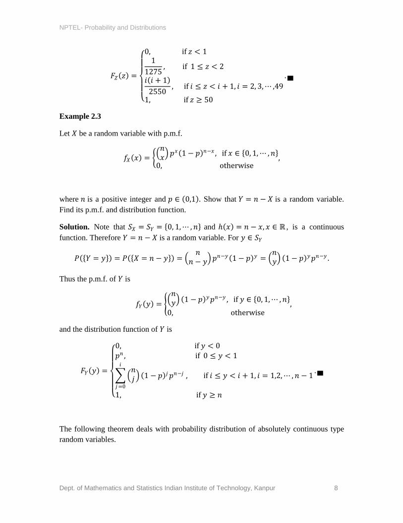
NPTEL- Probability and Distributions
Dept. of Mathematics and Statistics Indian Institute of Technology, Kanpur 8
𝐹𝑍 𝑧 =
0, if 𝑧 < 11
1275, if 1 ≤ 𝑧 < 2
𝑖 𝑖 + 1
2550, if 𝑖 ≤ 𝑧 < 𝑖 + 1, 𝑖 = 2, 3,⋯ ,49
1, if 𝑧 ≥ 50
. ▄
Example 2.3
Let 𝑋 be a random variable with p.m.f.
𝑓𝑋 𝑥 = 𝑛𝑥 𝑝𝑥 1 − 𝑝 𝑛−𝑥 , if 𝑥 ∈ 0, 1,⋯ ,𝑛
0, otherwise
,
where 𝑛 is a positive integer and 𝑝 ∈ 0,1 . Show that 𝑌 = 𝑛 − 𝑋 is a random variable.
Find its p.m.f. and distribution function.
Solution. Note that 𝑆𝑋 = 𝑆𝑌 = 0, 1,⋯ , 𝑛 and ℎ 𝑥 = 𝑛 − 𝑥, 𝑥 ∈ ℝ , is a continuous
function. Therefore 𝑌 = 𝑛 − 𝑋 is a random variable. For 𝑦 ∈ 𝑆𝑌
𝑃 𝑌 = 𝑦 = 𝑃 𝑋 = 𝑛 − 𝑦 = 𝑛
𝑛 − 𝑦 𝑝𝑛−𝑦 1 − 𝑝 𝑦 =
𝑛𝑦 1 − 𝑝 𝑦𝑝𝑛−𝑦 .
Thus the p.m.f. of 𝑌 is
𝑓𝑌 𝑦 = 𝑛𝑦 1 − 𝑝 𝑦𝑝𝑛−𝑦 , if 𝑦 ∈ 0, 1,⋯ ,𝑛
0, otherwise,
and the distribution function of 𝑌 is
𝐹𝑌 𝑦 =
0, if 𝑦 < 0𝑝𝑛 , if 0 ≤ 𝑦 < 1
𝑛𝑗 1 − 𝑝 𝑗𝑝𝑛−𝑗
𝑖
𝑗=0
, if 𝑖 ≤ 𝑦 < 𝑖 + 1, 𝑖 = 1,2,⋯ ,𝑛 − 1
1, if 𝑦 ≥ 𝑛
. ▄
The following theorem deals with probability distribution of absolutely continuous type
random variables.

NPTEL- Probability and Distributions
Dept. of Mathematics and Statistics Indian Institute of Technology, Kanpur 9
Theorem 2.2
Let 𝑋 be a random variable of absolutely continuous type with p.d.f. 𝑓𝑋(⋅) and support
𝑆𝑋 . Let 𝑆1, 𝑆2,⋯ , 𝑆𝑘 , be open intervals in ℝ such that 𝑆𝑖 ∩ 𝑆𝑗 = 𝜙, if 𝑖 ≠ 𝑗 and 𝑆𝑖 =𝑘𝑖=1
𝑆𝑋 . Let ℎ:ℝ → ℝ be a Borel function such that, on each 𝑆𝑖 𝑖 = 1,… ,𝑘 ,ℎ: 𝑆𝑖 → ℝ is
strictly monotone and continuously differentiable with inverse function ℎ𝑖−1(⋅) . Let
ℎ 𝑆𝑗 = ℎ 𝑥 :𝑥 ∈ 𝑆𝑗 so that ℎ 𝑆𝑗 𝑗 = 1,… ,𝑘 is an open interval in ℝ . Then the
random variable 𝑇 = ℎ 𝑋 is of absolutely continuous type with p.d.f.
𝑓𝑇 𝑡 = 𝑓𝑋
𝑘
𝑗=1
ℎ𝑗−1 𝑡
𝑑
𝑑𝑡ℎ𝑗−1 𝑡 𝐼ℎ 𝑆𝑗 (𝑡).
Proof. We will provide an outline of the proof which may not be rigorous. Let 𝐹𝑇(⋅) be
the distribution function of 𝑇. For 𝑡 ∈ ℝ and Δ > 0,
𝐹𝑇 𝑡 + Δ − 𝐹𝑇 𝑡
Δ=𝑃 𝑡 < ℎ 𝑋 ≤ 𝑡 + Δ
Δ
= 𝑃 𝑡 < ℎ 𝑋 ≤ 𝑡 + Δ,𝑋 ∈ 𝑆𝑗
Δ
𝑘
𝑗=1
∙
Fix 𝑗 ∈ 1,… ,𝑘 . First suppose that ℎ𝑗 (⋅) is strictly decreasing on 𝑆𝑗 . Note that 𝑋 ∈
𝑆𝑗 = ℎ 𝑋 ∈ ℎ 𝑆𝑗 and ℎ 𝑆𝑗 is an open interval. Thus, for 𝑡 belonging to the exterior
of ℎ 𝑆𝑗 and sufficiently small Δ > 0 , we have 𝑃 𝑡 < ℎ 𝑋 ≤ 𝑡 + Δ,𝑋 ∈ 𝑆𝑗 = 0.
Also, for 𝑡 ∈ ℎ 𝑆𝑗 and sufficiently small Δ > 0,
𝑃 𝑡 < ℎ 𝑋 ≤ 𝑡 + Δ,𝑋 ∈ 𝑆𝑗 = 𝑃 ℎ𝑗−1 𝑡 + Δ ≤ 𝑋 < ℎ𝑗
−1 𝑡 .
Thus, for all 𝑡 ∈ ℝ, we have
𝑃 𝑡 < ℎ 𝑋 ≤ 𝑡 + Δ,𝑋 ∈ 𝑆𝑗
Δ=𝑃 ℎ𝑗
−1 𝑡 + Δ ≤ 𝑋 < ℎ𝑗−1 𝑡 𝐼ℎ 𝑆𝑗 (𝑡)
Δ
=1
Δ 𝑓𝑋 𝑧 𝑑𝑧
ℎ𝑗−1(𝑡)
ℎ𝑗−1(𝑡+Δ)
𝐼ℎ 𝑆𝑗 (𝑡)
Δ↓0 −𝑓𝑋 ℎ𝑗
−1 𝑡 𝑑
𝑑𝑡ℎ𝑗−1 𝑡 𝐼ℎ 𝑆𝑗 𝑡 . (2.1)
Similarly if ℎ𝑗 is strictly increasing on 𝑆𝑗 then, for all 𝑡 ∈ ℝ, we have

NPTEL- Probability and Distributions
Dept. of Mathematics and Statistics Indian Institute of Technology, Kanpur 10
𝑃 𝑡 < ℎ 𝑋 ≤ 𝑡 + Δ,𝑋 ∈ 𝑆𝑗
Δ=𝑃 ℎ𝑗
−1 𝑡 < 𝑋 ≤ ℎ𝑗−1 𝑡 + Δ 𝐼ℎ 𝑆𝑗 (𝑡)
Δ
=1
Δ 𝑓𝑋 𝑧 𝑑𝑧
ℎ𝑗−1(𝑡+Δ)
ℎ𝑗−1(𝑡)
𝐼ℎ 𝑆𝑗 (𝑡)
Δ↓0 𝑓𝑋 ℎ𝑗
−1 𝑡 𝑑
𝑑𝑡ℎ𝑗−1 𝑡 𝐼ℎ 𝑆𝑗 𝑡 . (2.2)
Note that if ℎ is strictly decreasing (increasing) on 𝑆𝑗 then 𝑑
𝑑𝑡ℎ𝑗−1 𝑡 < > 0 on 𝑆𝑗 . Now
on combining (2.1) and (2.2) we get, for all 𝑡 ∈ ℝ,
𝑃 𝑡 < ℎ 𝑋 ≤ 𝑡 + Δ,𝑋 ∈ 𝑆𝑗
Δ
Δ↓0 𝑓𝑋 ℎ𝑗
−1 𝑡 𝑑
𝑑𝑡ℎ𝑗−1 𝑡 𝐼ℎ 𝑆𝑗 𝑡 ,
⇒𝐹𝑇 𝑡 + Δ − 𝐹𝑇 𝑡
Δ
Δ↓0 𝑓𝑋 ℎ𝑗
−1 𝑡
𝑘
𝑗=1
𝑑
𝑑𝑡ℎ𝑗−1 𝑡 𝐼ℎ 𝑆𝑗 𝑡 .
Similarly one can show that, for all 𝑡 ∈ ℝ,
limΔ↑0
𝐹𝑇 𝑡 + Δ − 𝐹𝑇 𝑡
Δ= 𝑓𝑋 ℎ𝑗
−1 𝑡
𝑘
𝑗=1
𝑑
𝑑𝑡ℎ𝑗−1 𝑡 𝐼ℎ 𝑆𝑗 𝑡 . (2.3)
It follows that the distribution function of 𝑇 is differentiable everywhere on ℝ except
possibly at a finite number of points (on boundaries of intervals ℎ 𝑆1 ,⋯ , ℎ 𝑆𝑘 of 𝑆𝑇).
Now the result follows from Remark 4.2 (vii) of Module 2 and using (2.3). ▄
The following corollary to the above theorem is immediate.
Corollary 2.2
Let 𝑋 be a random variable of absolutely continuous type with p.d.f. 𝑓𝑋(⋅) and support
𝑆𝑋 . Suppose that 𝑆𝑋 is a finite union of disjoint open intervals in ℝ and let ℎ:ℝ → ℝ be a
Borel function such that ℎ is differentiable and strictly monotone on 𝑆𝑋 (i.e., either
ℎ′ 𝑥 < 0,∀𝑥 ∈ 𝑆𝑋 or ℎ′ 𝑥 > 0,∀𝑥 ∈ 𝑆𝑋). Let 𝑆𝑇 = ℎ 𝑥 :𝑥 ∈ 𝑆𝑋 . Then 𝑇 = ℎ 𝑋 is a
random variable of absolutely continuous type with p.d.f.
𝑓𝑇 𝑡 = 𝑓𝑋 ℎ−1 𝑡
𝑑
𝑑𝑡ℎ−1 𝑡 , if 𝑡 ∈ 𝑆𝑇
0, otherwise∙ ▄
NPTEL- Probability and Distributions
Dept. of Mathematics and Statistics Indian Institute of Technology, Kanpur 11
It may be worth mentioning here that, in view of Remark 4.2 (vii) of Module 2, Theorem
2.2 and Corollary 2.2 can be applied even in situations where the function ℎ is
differentiable everywhere on 𝑆𝑋 except possibly at a finite number of points.
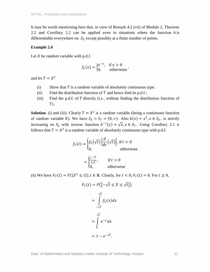
Example 2.4
Let 𝑋 be random variable with p.d.f.
𝑓𝑋 𝑥 = 𝑒−𝑥 , if 𝑥 > 00, otherwise
,
and let 𝑇 = 𝑋2
(i) Show that 𝑇 is a random variable of absolutely continuous type;
(ii) Find the distribution function of 𝑇 and hence find its p.d.f.;
(iii) Find the p.d.f. of 𝑇 directly (i.e., without finding the distribution function of
𝑇).
Solution. (i) and (iii). Clearly 𝑇 = 𝑋2 is a random variable (being a continuous function
of random variable 𝑋). We have 𝑆𝑋 = 𝑆𝑇 = 0, ∞ . Also ℎ 𝑥 = 𝑥2, 𝑥 ∈ 𝑆𝑋 , is strictly
increasing on 𝑆𝑋 with inverse function ℎ−1 𝑥 = 𝑥, 𝑥 ∈ 𝑆𝑇 . Using Corollary 2.1 it
follows that 𝑇 = 𝑋2 is a random variable of absolutely continuous type with p.d.f.
𝑓𝑇 𝑡 = 𝑓𝑋 𝑡 𝑑
𝑑𝑡 𝑡 , if 𝑡 > 0
0, otherwise
= 𝑒− 𝑡
2 𝑡, if 𝑡 > 0
0, otherwise
.
(ii) We have 𝐹𝑇 𝑡 = 𝑃 𝑋2 ≤ 𝑡 , 𝑡 ∈ ℝ. Clearly, for 𝑡 < 0,𝐹𝑇 𝑡 = 0. For 𝑡 ≥ 0,
𝐹𝑇 𝑡 = 𝑃 − 𝑡 ≤ 𝑋 ≤ 𝑡
= 𝑓𝑋 𝑥 𝑑𝑥
𝑡
− 𝑡
= 𝑒−𝑥𝑑𝑥
𝑡
0
= 1 − 𝑒− 𝑡 .
NPTEL- Probability and Distributions
Dept. of Mathematics and Statistics Indian Institute of Technology, Kanpur 12
Therefore the distribution function of 𝑇 is
𝐹𝑇 𝑡 = 0, if 𝑡 < 0
1 − 𝑒− 𝑡 , if 𝑡 ≥ 0 .
Clearly 𝐹𝑇 is differentiable everywhere except at 𝑡 = 0. Therefore, using Remark 4.2
(vii) of Module 2, we conclude that the random variable 𝑇 is of absolutely continuous
type with p.d.f. 𝑓𝑇 𝑡 = 𝐹𝑇′ 𝑡 , if 𝑡 ≠ 0 . At 𝑡 = 0 we may assign any arbitrary non-
negative value to 𝑓𝑇 0 . Thus a p.d.f. of 𝑇 is
𝑓𝑇 𝑡 = 𝑒− 𝑡
2 𝑡, if 𝑡 > 0
0, otherwise
. ▄
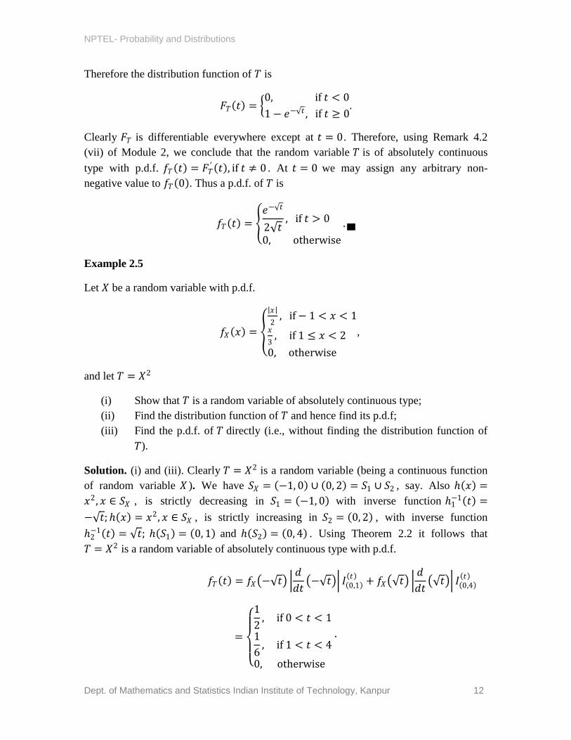
Example 2.5
Let 𝑋 be a random variable with p.d.f.
𝑓𝑋 𝑥 =
𝑥
2, if − 1 < 𝑥 < 1
𝑥
3, if 1 ≤ 𝑥 < 2
0, otherwise
,
and let 𝑇 = 𝑋2
(i) Show that 𝑇 is a random variable of absolutely continuous type;
(ii) Find the distribution function of 𝑇 and hence find its p.d.f;
(iii) Find the p.d.f. of 𝑇 directly (i.e., without finding the distribution function of
𝑇).
Solution. (i) and (iii). Clearly 𝑇 = 𝑋2 is a random variable (being a continuous function
of random variable 𝑋 ). We have 𝑆𝑋 = −1, 0 ∪ 0, 2 = 𝑆1 ∪ 𝑆2 , say. Also ℎ 𝑥 =
𝑥2 , 𝑥 ∈ 𝑆𝑋 , is strictly decreasing in 𝑆1 = −1, 0 with inverse function ℎ1−1 𝑡 =
− 𝑡;ℎ 𝑥 = 𝑥2 , 𝑥 ∈ 𝑆𝑋 , is strictly increasing in 𝑆2 = 0, 2 , with inverse function
ℎ2−1 𝑡 = 𝑡; ℎ 𝑆1 = 0, 1 and ℎ 𝑆2 = 0, 4 . Using Theorem 2.2 it follows that
𝑇 = 𝑋2 is a random variable of absolutely continuous type with p.d.f.
𝑓𝑇 𝑡 = 𝑓𝑋 − 𝑡 𝑑
𝑑𝑡 − 𝑡 𝐼 0,1
𝑡 + 𝑓𝑋 𝑡 𝑑
𝑑𝑡 𝑡 𝐼 0,4
𝑡
=
1
2, if 0 < 𝑡 < 1
1
6, if 1 < 𝑡 < 4
0, otherwise
∙

NPTEL- Probability and Distributions
Dept. of Mathematics and Statistics Indian Institute of Technology, Kanpur 13
(ii) We have 𝐹𝑇 𝑡 = 𝑃 𝑋2 ≤ 𝑡 , 𝑡 ∈ ℝ . Since 𝑃 𝑋 ∈ −1, 2 = 1 , we have
𝑃 𝑇 ∈ 0, 4 = 1.
Therefore, for 𝑡 < 0, 𝐹𝑇 𝑡 = 𝑃 𝑇 ≤ 𝑡 = 0 and, for 𝑡 ≥ 4, 𝐹𝑇 𝑡 = 𝑃 𝑇 ≤ 𝑡 = 1.
For 𝑡 ∈ [0,4), we have
𝐹𝑇 𝑡 = 𝑃 − 𝑡 ≤ 𝑋 ≤ 𝑡
= 𝑓𝑋 𝑥
𝑡
− 𝑡
𝑑𝑥
=
|𝑥|
2𝑑𝑥, if 0 ≤ 𝑡 < 1
𝑡
− 𝑡
|𝑥|
2𝑑𝑥
1
−1
+ 𝑥
3𝑑𝑥,
𝑡
1
if 1 ≤ 𝑡 < 4
.
Therefore, the distribution function of 𝑇 is
𝐹𝑇 𝑡 =
0, if 𝑡 < 0𝑡
2, if 0 ≤ 𝑡 < 1
𝑡 + 2
6, if 1 ≤ 𝑡 < 4
1, if 𝑡 ≥ 4
∙
Clearly 𝐹𝑇 is differentiable everywhere except at points 0, 1 and 4. Using Remark 4.2
(vii) of Module 2 it follows that the random variable 𝑇 is of absolutely continuous type
with a p.d.f.
𝑓𝑇 𝑡 =
1
2, if 0 < 𝑡 < 1
1
6, if 1 < 𝑡 < 4
0, otherwise
∙ ▄
Note that a Borel function of a discrete type random variable is a random variable of
discrete type (see Theorem 1.1). Theorem 2.2 provides sufficient conditions under which
a Borel function of an absolutely continuous type random variable is of absolutely
continuous type. The following example illustrates that, in general, a Borel function of an
absolutely continuous type random variable may not be of absolutely continuous type.
NPTEL- Probability and Distributions
Dept. of Mathematics and Statistics Indian Institute of Technology, Kanpur 14
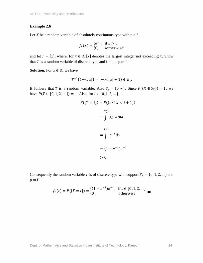
Example 2.6
Let 𝑋 be a random variable of absolutely continuous type with p.d.f.
𝑓𝑋 𝑥 = 𝑒−𝑥 , if 𝑥 > 00, 𝑠otherwise
,
and let 𝑇 = 𝑥 , where, for 𝑥 ∈ ℝ, 𝑥 denotes the largest integer not exceeding 𝑥. Show
that 𝑇 is a random variable of discrete type and find its p.m.f.
Solution. For 𝑎 ∈ ℝ, we have
𝑇−1 −∞,𝑎 = −∞, 𝑎 + 1 ∈ ℬ1.
It follows that 𝑇 is a random variable. Also 𝑆𝑋 = 0, ∞ . Since 𝑃 𝑋 ∈ 𝑆𝑋 = 1 , we
have 𝑃 𝑇 ∈ 0, 1, 2,⋯ = 1. Also, for 𝑖 ∈ 0, 1, 2,… .
𝑃 𝑇 = 𝑖 = 𝑃( 𝑖 ≤ 𝑋 < 𝑖 + 1 )
= 𝑓𝑋 𝑥 𝑑𝑥
𝑖+1
𝑖
= 𝑒−𝑥𝑑𝑥
𝑖+1
𝑖
= 1 − 𝑒−1 𝑒−𝑖
> 0.
Consequently the random variable 𝑇 is of discrete type with support 𝑆𝑇 = 0, 1, 2,… and
p.m.f.
𝑓𝑇 𝑡 = 𝑃 𝑇 = 𝑡 = 1 − 𝑒−1 𝑒−𝑡 , if 𝑡 ∈ 0 ,1, 2,… 0 , otherwise
. ▄