Embed Size (px)
Citation preview
DEPT OF CSE & IT
VSSUT, Burla
LECTURE NOTES
ON
SOFTWARE ENGINEERING
Course Code: BCS-306
By
Dr. H.S.Behera
Asst. Prof K.K.Sahu
Asst. Prof Gargi Bhattacharjee
DEPT OF CSE & IT
VSSUT, Burla
DISCLAIMER
THIS DOCUMENT DOES NOT CLAIM ANY ORIGINALITY AND
CANNOT BE USED AS A SUBSTITUTE FOR PRESCRIBED
TEXTBOOKS. THE INFORMATION PRESENTED HERE IS
MERELY A COLLECTION BY THE COMMITTEE MEMBERS FOR
THEIR RESPECTIVE TEACHING ASSIGNMENTS. VARIOUS
TEXT BOOKS AS WELL AS FREELY AVAILABLE MATERIAL
FROM INTERNET WERE CONSULTED FOR PREPARING THIS
DOCUMENT. THE OWNERSHIP OF THE INFORMATION LIES
WITH THE RESPECTIVE AUTHORS OR INSTITUTIONS.
DEPT OF CSE & IT
VSSUT, Burla
SYLLABUS
Module I:
Introductory concepts: Introduction, definition, objectives, Life cycle – Requirements analysis
and specification. Design and Analysis: Cohesion and coupling, Data flow oriented Design:
Transform centered design, Transaction centered design. Analysis of specific systems like
Inventory control, Reservation system.
Module II:
Object-oriented Design: Object modeling using UML, use case diagram, class diagram,
interaction diagrams: activity diagram, unified development process.
Module III:
Implementing and Testing: Programming language characteristics, fundamentals, languages,
classes, coding style efficiency. Testing: Objectives, black box and white box testing, various
testing strategies, Art of debugging. Maintenance, Reliability and Availability: Maintenance:
Characteristics, controlling factors, maintenance tasks, side effects, preventive maintenance – Re
Engineering – Reverse Engineering – configuration management – Maintenance tools and
techniques. Reliability: Concepts, Errors, Faults, Repair and availability, reliability and
availability models. Recent trends and developments.
Module IV:
Software quality: SEI CMM and ISO-9001. Software reliability and fault-tolerance, software
project planning, monitoring, and control. Computer-aided software engineering (CASE),
Component model of software development, Software reuse.
Text Book:
1. Mall Rajib, Fundamentals of Software Engineering, PHI.
2. Pressman, Software Engineering Practitioner’s Approach, TMH.

DEPT OF CSE & IT
VSSUT, Burla
CONTENTS
Module 1:
Lecture 1: Introduction to Software Engineering
Lecture 2: Software Development Life Cycle- Classical Waterfall Model
Lecture 3: Iterative Waterfall Model, Prototyping Model, Evolutionary Model
Lecture 4: Spiral Model
Lecture 5: Requirements Analysis and Specification
Lecture 6: Problems without a SRS document, Decision Tree, Decision Table
Lecture 7: Formal System Specification
Lecture 8: Software Design
Lecture 9: Software Design Strategies
Lecture 10: Software Analysis & Design Tools
Lecture 11: Structured Design
Module 2:
Lecture 12: Object Modelling Using UML
Lecture 13: Use Case Diagram
Lecture 14: Class Diagrams
Lecture 15: Interaction Diagrams
Lecture 16: Activity and State Chart Diagram
DEPT OF CSE & IT
VSSUT, Burla
Module 3:
Lecture 17: Coding
Lecture 18: Testing
Lecture 19: Black-Box Testing
Lecture 20: White-Box Testing
Lecture 21: White-Box Testing (cont..)
Lecture 22: Debugging, Integration and System Testing
Lecture 23: Integration Testing
Lecture 24: Software Maintenance
Lecture 25: Software Maintenance Process Models
Lecture 26: Software Reliability and Quality Management
Lecture 27: Reliability Growth Models
Module 4:
Lecture 28: Software Quality
Lecture 29: SEI Capability Maturity Model
Lecture 30: Software Project Planning
Lecture 31: Metrics for Software Project Size Estimation
Lecture 32: Heuristic Techniques, Analytical Estimation Techniques
Lecture 33: COCOMO Model
Lecture 34: Intermediate COCOMO Model
Lecture 35: Staffing Level Estimation
DEPT OF CSE & IT
VSSUT, Burla
Lecture 36: Project Scheduling
Lecture 37: Organization Structure
Lecture 38: Risk Management
Lecture 39: Computer Aided Software Engineering
Lecture 40: Software Reuse
Lecture 41: Reuse Approach
References
DEPT OF CSE & IT
VSSUT, Burla
MODULE 1
LECTURE NOTE 1
INTRODUCTION TO SOFTWARE ENGINEERING
The term software engineering is composed of two words, software and engineering.
Software is more than just a program code. A program is an executable code, which serves
some computational purpose. Software is considered to be a collection of executable
programming code, associated libraries and documentations. Software, when made for a
specific requirement is called software product.
Engineering on the other hand, is all about developing products, using well-defined, scientific
principles and methods.
So, we can define software engineering as an engineering branch associated with the
development of software product using well-defined scientific principles, methods and
procedures. The outcome of software engineering is an efficient and reliable software product.
IEEE defines software engineering as:
The application of a systematic, disciplined, quantifiable approach to the development,
operation and maintenance of software.
We can alternatively view it as a systematic collection of past experience. The experience is
arranged in the form of methodologies and guidelines. A small program can be written without
using software engineering principles. But if one wants to develop a large software product, then
software engineering principles are absolutely necessary to achieve a good quality software cost
effectively.
Without using software engineering principles it would be difficult to develop large programs. In
industry it is usually needed to develop large programs to accommodate multiple functions. A
problem with developing such large commercial programs is that the complexity and difficulty
levels of the programs increase exponentially with their sizes. Software engineering helps to
reduce this programming complexity. Software engineering principles use two important
techniques to reduce problem complexity: abstraction and decomposition. The principle of
abstraction implies that a problem can be simplified by omitting irrelevant details. In other
words, the main purpose of abstraction is to consider only those aspects of the problem that are
relevant for certain purpose and suppress other aspects that are not relevant for the given
purpose. Once the simpler problem is solved, then the omitted details can be taken into
consideration to solve the next lower level abstraction, and so on. Abstraction is a powerful way
of reducing the complexity of the problem. The other approach to tackle problem complexity is

DEPT OF CSE & IT
VSSUT, Burla
decomposition. In this technique, a complex problem is divided into several smaller problems
and then the smaller problems are solved one by one. However, in this technique any random
decomposition of a problem into smaller parts will not help. The problem has to be decomposed
such that each component of the decomposed problem can be solved independently and then the
solution of the different components can be combined to get the full solution. A good
decomposition of a problem should minimize interactions among various components. If the
different subcomponents are interrelated, then the different components cannot be solved
separately and the desired reduction in complexity will not be realized.
NEED OF SOFTWARE ENGINEERING
The need of software engineering arises because of higher rate of change in user requirements
and environment on which the software is working.
Large software - It is easier to build a wall than to a house or building, likewise, as the
size of software become large engineering has to step to give it a scientific process.
Scalability- If the software process were not based on scientific and engineering
concepts, it would be easier to re-create new software than to scale an existing one.
Cost- As hardware industry has shown its skills and huge manufacturing has lower down
the price of computer and electronic hardware. But the cost of software remains high if
proper process is not adapted.
Dynamic Nature- The always growing and adapting nature of software hugely depends
upon the environment in which the user works. If the nature of software is always
changing, new enhancements need to be done in the existing one. This is where software
engineering plays a good role.
Quality Management- Better process of software development provides better and
quality software product.
CHARACTERESTICS OF GOOD SOFTWARE
A software product can be judged by what it offers and how well it can be used. This software
must satisfy on the following grounds:
Operational
Transitional
Maintenance

DEPT OF CSE & IT
VSSUT, Burla
Well-engineered and crafted software is expected to have the following characteristics:
Operational
This tells us how well software works in operations. It can be measured on:
Budget
Usability
Efficiency
Correctness
Functionality
Dependability
Security
Safety
Transitional
This aspect is important when the software is moved from one platform to another:
Portability
Interoperability
Reusability
Adaptability
Maintenance
This aspect briefs about how well a software has the capabilities to maintain itself in the ever-
changing environment:
Modularity
Maintainability
Flexibility
Scalability
In short, Software engineering is a branch of computer science, which uses well-defined
engineering concepts required to produce efficient, durable, scalable, in-budget and on-time
software products
DEPT OF CSE & IT
VSSUT, Burla
LECTURE NOTE 2
SOFTWARE DEVELOPMENT LIFE CYCLE
LIFE CYCLE MODEL
A software life cycle model (also called process model) is a descriptive and diagrammatic
representation of the software life cycle. A life cycle model represents all the activities required
to make a software product transit through its life cycle phases. It also captures the order in
which these activities are to be undertaken. In other words, a life cycle model maps the different
activities performed on a software product from its inception to retirement. Different life cycle
models may map the basic development activities to phases in different ways. Thus, no matter
which life cycle model is followed, the basic activities are included in all life cycle models
though the activities may be carried out in different orders in different life cycle models. During
any life cycle phase, more than one activity may also be carried out.
THE NEED FOR A SOFTWARE LIFE CYCLE MODEL
The development team must identify a suitable life cycle model for the particular project and
then adhere to it. Without using of a particular life cycle model the development of a software
product would not be in a systematic and disciplined manner. When a software product is being
developed by a team there must be a clear understanding among team members about when and
what to do. Otherwise it would lead to chaos and project failure. This problem can be illustrated
by using an example. Suppose a software development problem is divided into several parts and
the parts are assigned to the team members. From then on, suppose the team members are
allowed the freedom to develop the parts assigned to them in whatever way they like. It is
possible that one member might start writing the code for his part, another might decide to
prepare the test documents first, and some other engineer might begin with the design phase of
the parts assigned to him. This would be one of the perfect recipes for project failure. A software
life cycle model defines entry and exit criteria for every phase. A phase can start only if its
phase-entry criteria have been satisfied. So without software life cycle model the entry and exit
criteria for a phase cannot be recognized. Without software life cycle models it becomes difficult
for software project managers to monitor the progress of the project.
Different software life cycle models
Many life cycle models have been proposed so far. Each of them has some advantages as well as
some disadvantages. A few important and commonly used life cycle models are as follows:
Classical Waterfall Model

DEPT OF CSE & IT
VSSUT, Burla
Iterative Waterfall Model
Prototyping Model
Evolutionary Model
Spiral Model
1. CLASSICAL WATERFALL MODEL
The classical waterfall model is intuitively the most obvious way to develop software. Though
the classical waterfall model is elegant and intuitively obvious, it is not a practical model in the
sense that it cannot be used in actual software development projects. Thus, this model can be
considered to be a theoretical way of developing software. But all other life cycle models are
essentially derived from the classical waterfall model. So, in order to be able to appreciate other
life cycle models it is necessary to learn the classical waterfall model. Classical waterfall model
divides the life cycle into the following phases as shown in fig.2.1:
Fig 2.1: Classical Waterfall Model
Feasibility study - The main aim of feasibility study is to determine whether it would be
financially and technically feasible to develop the product.
DEPT OF CSE & IT
VSSUT, Burla
At first project managers or team leaders try to have a rough understanding of what is
required to be done by visiting the client side. They study different input data to the
system and output data to be produced by the system. They study what kind of processing
is needed to be done on these data and they look at the various constraints on the
behavior of the system.
After they have an overall understanding of the problem they investigate the different
solutions that are possible. Then they examine each of the solutions in terms of what kind
of resources required, what would be the cost of development and what would be the
development time for each solution.
Based on this analysis they pick the best solution and determine whether the solution is
feasible financially and technically. They check whether the customer budget would meet
the cost of the product and whether they have sufficient technical expertise in the area of
development.
Requirements analysis and specification: - The aim of the requirements analysis and
specification phase is to understand the exact requirements of the customer and to document
them properly. This phase consists of two distinct activities, namely
Requirements gathering and analysis
Requirements specification
The goal of the requirements gathering activity is to collect all relevant information from the
customer regarding the product to be developed. This is done to clearly understand the customer
requirements so that incompleteness and inconsistencies are removed.
The requirements analysis activity is begun by collecting all relevant data regarding the product
to be developed from the users of the product and from the customer through interviews and
discussions. For example, to perform the requirements analysis of a business accounting software
required by an organization, the analyst might interview all the accountants of the organization to
ascertain their requirements. The data collected from such a group of users usually contain
several contradictions and ambiguities, since each user typically has only a partial and
incomplete view of the system. Therefore it is necessary to identify all ambiguities and
contradictions in the requirements and resolve them through further discussions with the
customer. After all ambiguities, inconsistencies, and incompleteness have been resolved and all
the requirements properly understood, the requirements specification activity can start. During
this activity, the user requirements are systematically organized into a Software Requirements
Specification (SRS) document. The customer requirements identified during the requirements
gathering and analysis activity are organized into a SRS document. The important components of
this document are functional requirements, the nonfunctional requirements, and the goals of
implementation.
DEPT OF CSE & IT
VSSUT, Burla
Design: - The goal of the design phase is to transform the requirements specified in the SRS
document into a structure that is suitable for implementation in some programming language. In
technical terms, during the design phase the software architecture is derived from the SRS
document. Two distinctly different approaches are available: the traditional design approach and
the object-oriented design approach.
Traditional design approach -Traditional design consists of two different activities; first
a structured analysis of the requirements specification is carried out where the detailed
structure of the problem is examined. This is followed by a structured design activity.
During structured design, the results of structured analysis are transformed into the
software design.
Object-oriented design approach -In this technique, various objects that occur in the
problem domain and the solution domain are first identified, and the different
relationships that exist among these objects are identified. The object structure is further
refined to obtain the detailed design.
Coding and unit testing:-The purpose of the coding phase (sometimes called the
implementation phase) of software development is to translate the software design into source
code. Each component of the design is implemented as a program module. The end-product of
this phase is a set of program modules that have been individually tested. During this phase, each
module is unit tested to determine the correct working of all the individual modules. It involves
testing each module in isolation as this is the most efficient way to debug the errors identified at
this stage.
Integration and system testing: -Integration of different modules is undertaken once they have
been coded and unit tested. During the integration and system testing phase, the modules are
integrated in a planned manner. The different modules making up a software product are almost
never integrated in one shot. Integration is normally carried out incrementally over a number of
steps. During each integration step, the partially integrated system is tested and a set of
previously planned modules are added to it. Finally, when all the modules have been successfully
integrated and tested, system testing is carried out. The goal of system testing is to ensure that
the developed system conforms to its requirements laid out in the SRS document. System testing
usually consists of three different kinds of testing activities:
α – testing: It is the system testing performed by the development team.
β –testing: It is the system testing performed by a friendly set of customers.
Acceptance testing: It is the system testing performed by the customer himself after the
product delivery to determine whether to accept or reject the delivered product.
System testing is normally carried out in a planned manner according to the system test plan
document. The system test plan identifies all testing-related activities that must be performed,
DEPT OF CSE & IT
VSSUT, Burla
specifies the schedule of testing, and allocates resources. It also lists all the test cases and the
expected outputs for each test case.
Maintenance: -Maintenance of a typical software product requires much more than the effort
necessary to develop the product itself. Many studies carried out in the past confirm this and
indicate that the relative effort of development of a typical software product to its maintenance
effort is roughly in the 40:60 ratios. Maintenance involves performing any one or more of the
following three kinds of activities:
Correcting errors that were not discovered during the product development phase. This is
called corrective maintenance.
Improving the implementation of the system, and enhancing the functionalities of the
system according to the customer’s requirements. This is called perfective maintenance.
Porting the software to work in a new environment. For example, porting may be
required to get the software to work on a new computer platform or with a new operating
system. This is called adaptive maintenance.
Shortcomings of the classical waterfall model
The classical waterfall model is an idealistic one since it assumes that no development error is
ever committed by the engineers during any of the life cycle phases. However, in practical
development environments, the engineers do commit a large number of errors in almost every
phase of the life cycle. The source of the defects can be many: oversight, wrong assumptions, use
of inappropriate technology, communication gap among the project engineers, etc. These defects
usually get detected much later in the life cycle. For example, a design defect might go unnoticed
till we reach the coding or testing phase. Once a defect is detected, the engineers need to go back
to the phase where the defect had occurred and redo some of the work done during that phase
and the subsequent phases to correct the defect and its effect on the later phases. Therefore, in
any practical software development work, it is not possible to strictly follow the classical
waterfall model.
DEPT OF CSE & IT
VSSUT, Burla
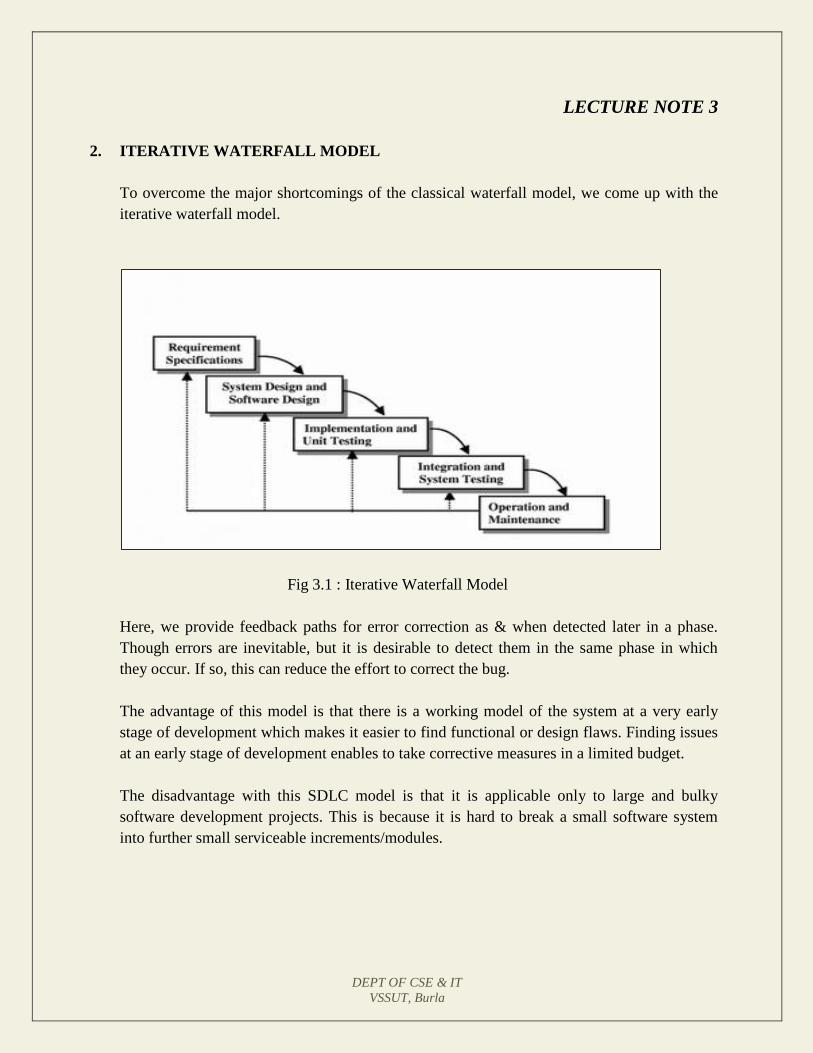
LECTURE NOTE 3
2. ITERATIVE WATERFALL MODEL
To overcome the major shortcomings of the classical waterfall model, we come up with the
iterative waterfall model.
Fig 3.1 : Iterative Waterfall Model
Here, we provide feedback paths for error correction as & when detected later in a phase.
Though errors are inevitable, but it is desirable to detect them in the same phase in which
they occur. If so, this can reduce the effort to correct the bug.
The advantage of this model is that there is a working model of the system at a very early
stage of development which makes it easier to find functional or design flaws. Finding issues
at an early stage of development enables to take corrective measures in a limited budget.
The disadvantage with this SDLC model is that it is applicable only to large and bulky
software development projects. This is because it is hard to break a small software system
into further small serviceable increments/modules.

DEPT OF CSE & IT
VSSUT, Burla
3. PRTOTYPING MODEL
Prototype
A prototype is a toy implementation of the system. A prototype usually exhibits limited
functional capabilities, low reliability, and inefficient performance compared to the actual
software. A prototype is usually built using several shortcuts. The shortcuts might involve
using inefficient, inaccurate, or dummy functions. The shortcut implementation of a function,
for example, may produce the desired results by using a table look-up instead of performing
the actual computations. A prototype usually turns out to be a very crude version of the
actual system.
Need for a prototype in software development
There are several uses of a prototype. An important purpose is to illustrate the input data
formats, messages, reports, and the interactive dialogues to the customer. This is a valuable
mechanism for gaining better understanding of the customer’s needs:
how the screens might look like
how the user interface would behave
how the system would produce outputs
Another reason for developing a prototype is that it is impossible to get the perfect product
in the first attempt. Many researchers and engineers advocate that if you want to develop a
good product you must plan to throw away the first version. The experience gained in
developing the prototype can be used to develop the final product.
A prototyping model can be used when technical solutions are unclear to the development
team. A developed prototype can help engineers to critically examine the technical issues
associated with the product development. Often, major design decisions depend on issues
like the response time of a hardware controller, or the efficiency of a sorting algorithm, etc.
In such circumstances, a prototype may be the best or the only way to resolve the technical
issues.
A prototype of the actual product is preferred in situations such as:
• User requirements are not complete
• Technical issues are not clear
DEPT OF CSE & IT
VSSUT, Burla
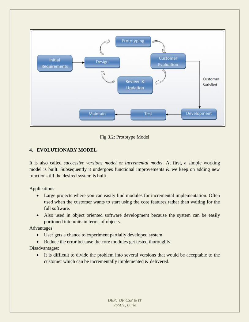
Fig 3.2: Prototype Model
4. EVOLUTIONARY MODEL
It is also called successive versions model or incremental model. At first, a simple working
model is built. Subsequently it undergoes functional improvements & we keep on adding new
functions till the desired system is built.
Applications:
Large projects where you can easily find modules for incremental implementation. Often
used when the customer wants to start using the core features rather than waiting for the
full software.
Also used in object oriented software development because the system can be easily
portioned into units in terms of objects.
Advantages:
User gets a chance to experiment partially developed system
Reduce the error because the core modules get tested thoroughly.
Disadvantages:
It is difficult to divide the problem into several versions that would be acceptable to the
customer which can be incrementally implemented & delivered.
DEPT OF CSE & IT
VSSUT, Burla
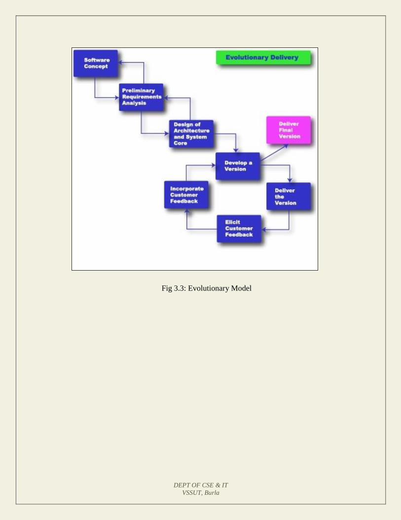
Fig 3.3: Evolutionary Model
DEPT OF CSE & IT
VSSUT, Burla
LECTURE NOTE 4
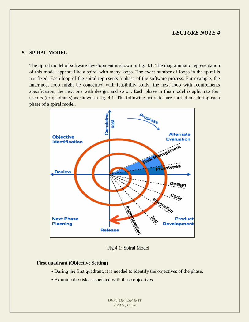
5. SPIRAL MODEL
The Spiral model of software development is shown in fig. 4.1. The diagrammatic representation
of this model appears like a spiral with many loops. The exact number of loops in the spiral is
not fixed. Each loop of the spiral represents a phase of the software process. For example, the
innermost loop might be concerned with feasibility study, the next loop with requirements
specification, the next one with design, and so on. Each phase in this model is split into four
sectors (or quadrants) as shown in fig. 4.1. The following activities are carried out during each
phase of a spiral model.
Fig 4.1: Spiral Model
First quadrant (Objective Setting)
• During the first quadrant, it is needed to identify the objectives of the phase.
• Examine the risks associated with these objectives.
DEPT OF CSE & IT
VSSUT, Burla
Second Quadrant (Risk Assessment and Reduction)
• A detailed analysis is carried out for each identified project risk.
• Steps are taken to reduce the risks. For example, if there is a risk that the
requirements are inappropriate, a prototype system may be developed.
Third Quadrant (Development and Validation)
• Develop and validate the next level of the product after resolving the identified
risks.
Fourth Quadrant (Review and Planning)
• Review the results achieved so far with the customer and plan the next iteration
around the spiral.
• Progressively more complete version of the software gets built with each iteration
around the spiral.
Circumstances to use spiral model
The spiral model is called a meta model since it encompasses all other life cycle models. Risk
handling is inherently built into this model. The spiral model is suitable for development of
technically challenging software products that are prone to several kinds of risks. However, this
model is much more complex than the other models – this is probably a factor deterring its use in
ordinary projects.
Comparison of different life-cycle models
The classical waterfall model can be considered as the basic model and all other life cycle
models as embellishments of this model. However, the classical waterfall model cannot be used
in practical development projects, since this model supports no mechanism to handle the errors
committed during any of the phases.
This problem is overcome in the iterative waterfall model. The iterative waterfall model is
probably the most widely used software development model evolved so far. This model is simple
to understand and use. However this model is suitable only for well-understood problems; it is
not suitable for very large projects and for projects that are subject to many risks.
The prototyping model is suitable for projects for which either the user requirements or the
underlying technical aspects are not well understood. This model is especially popular for
development of the user-interface part of the projects.

DEPT OF CSE & IT
VSSUT, Burla
The evolutionary approach is suitable for large problems which can be decomposed into a set of
modules for incremental development and delivery. This model is also widely used for object-
oriented development projects. Of course, this model can only be used if the incremental delivery
of the system is acceptable to the customer.
The spiral model is called a meta model since it encompasses all other life cycle models. Risk
handling is inherently built into this model. The spiral model is suitable for development of
technically challenging software products that are prone to several kinds of risks. However, this
model is much more complex than the other models – this is probably a factor deterring its use in
ordinary projects.
The different software life cycle models can be compared from the viewpoint of the customer.
Initially, customer confidence in the development team is usually high irrespective of the
development model followed. During the lengthy development process, customer confidence
normally drops off, as no working product is immediately visible. Developers answer customer
queries using technical slang, and delays are announced. This gives rise to customer resentment.
On the other hand, an evolutionary approach lets the customer experiment with a working
product much earlier than the monolithic approaches. Another important advantage of the
incremental model is that it reduces the customer’s trauma of getting used to an entirely new
system. The gradual introduction of the product via incremental phases provides time to the
customer to adjust to the new product. Also, from the customer’s financial viewpoint,
incremental development does not require a large upfront capital outlay. The customer can order
the incremental versions as and when he can afford them.
DEPT OF CSE & IT
VSSUT, Burla
LECTURE NOTE 5
REQUIREMENTS ANALYSIS AND SPECIFICATION
Before we start to develop our software, it becomes quite essential for us to understand and
document the exact requirement of the customer. Experienced members of the development team
carry out this job. They are called as system analysts.
The analyst starts requirements gathering and analysis activity by collecting all information
from the customer which could be used to develop the requirements of the system. He then
analyzes the collected information to obtain a clear and thorough understanding of the product to
be developed, with a view to remove all ambiguities and inconsistencies from the initial
customer perception of the problem. The following basic questions pertaining to the project
should be clearly understood by the analyst in order to obtain a good grasp of the problem:
• What is the problem?
• Why is it important to solve the problem?
• What are the possible solutions to the problem?
• What exactly are the data input to the system and what exactly are the data output by the
system?
• What are the likely complexities that might arise while solving the problem?
• If there are external software or hardware with which the developed software has to
interface, then what exactly would the data interchange formats with the external system
be?
After the analyst has understood the exact customer requirements, he proceeds to identify and
resolve the various requirements problems. The most important requirements problems that the
analyst has to identify and eliminate are the problems of anomalies, inconsistencies, and
incompleteness. When the analyst detects any inconsistencies, anomalies or incompleteness in
the gathered requirements, he resolves them by carrying out further discussions with the end-
users and the customers.
Parts of a SRS document
• The important parts of SRS document are:
Functional requirements of the system
Non-functional requirements of the system, and
Goals of implementation
DEPT OF CSE & IT
VSSUT, Burla
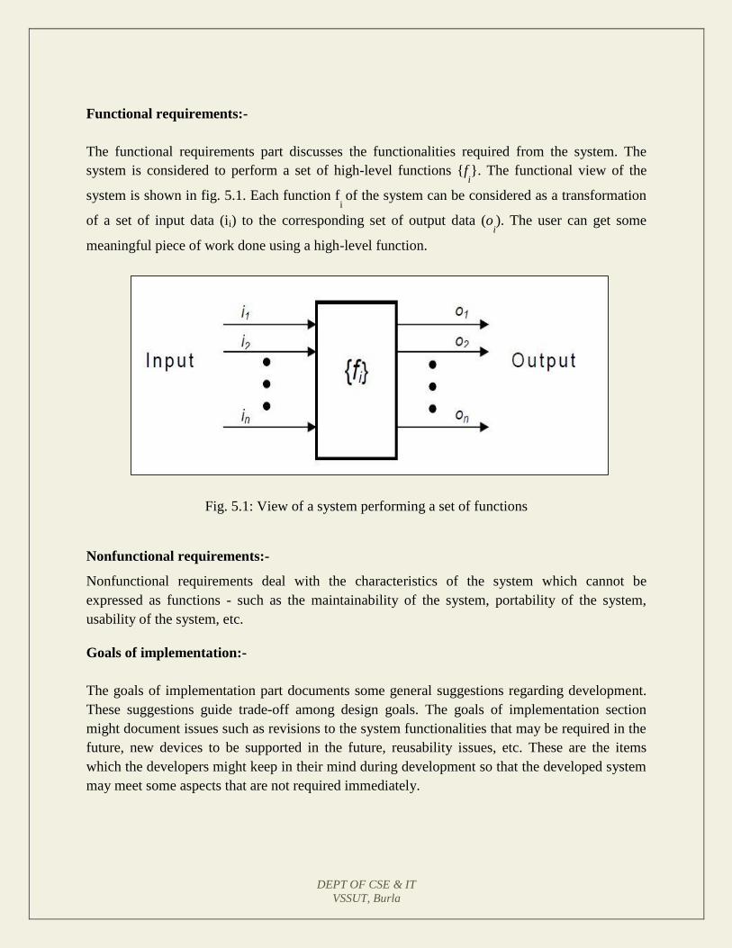
Functional requirements:-
The functional requirements part discusses the functionalities required from the system. The
system is considered to perform a set of high-level functions {fi}. The functional view of the
system is shown in fig. 5.1. Each function fi of the system can be considered as a transformation
of a set of input data (ii) to the corresponding set of output data (oi). The user can get some
meaningful piece of work done using a high-level function.
Fig. 5.1: View of a system performing a set of functions
Nonfunctional requirements:-
Nonfunctional requirements deal with the characteristics of the system which cannot be
expressed as functions - such as the maintainability of the system, portability of the system,
usability of the system, etc.
Goals of implementation:-
The goals of implementation part documents some general suggestions regarding development.
These suggestions guide trade-off among design goals. The goals of implementation section
might document issues such as revisions to the system functionalities that may be required in the
future, new devices to be supported in the future, reusability issues, etc. These are the items
which the developers might keep in their mind during development so that the developed system
may meet some aspects that are not required immediately.
DEPT OF CSE & IT
VSSUT, Burla
Identifying functional requirements from a problem description
The high-level functional requirements often need to be identified either from an informal
problem description document or from a conceptual understanding of the problem. Each high-
level requirement characterizes a way of system usage by some user to perform some meaningful
piece of work. There can be many types of users of a system and their requirements from the
system may be very different. So, it is often useful to identify the different types of users who
might use the system and then try to identify the requirements from each user’s perspective.
Example: - Consider the case of the library system, where –
F1: Search Book function
Input: an author’s name
Output: details of the author’s books and the location of these books in the library
So the function Search Book (F1) takes the author's name and transforms it into book details.
Functional requirements actually describe a set of high-level requirements, where each high-level
requirement takes some data from the user and provides some data to the user as an output. Also
each high-level requirement might consist of several other functions.
Documenting functional requirements
For documenting the functional requirements, we need to specify the set of functionalities
supported by the system. A function can be specified by identifying the state at which the data is
to be input to the system, its input data domain, the output data domain, and the type of
processing to be carried on the input data to obtain the output data. Let us first try to document
the withdraw-cash function of an ATM (Automated Teller Machine) system. The withdraw-cash
is a high-level requirement. It has several sub-requirements corresponding to the different user
interactions. These different interaction sequences capture the different scenarios.
Example: - Withdraw Cash from ATM
R1: withdraw cash
Description: The withdraw cash function first determines the type of account that the user has
and the account number from which the user wishes to withdraw cash. It checks the balance to
determine whether the requested amount is available in the account. If enough balance is
available, it outputs the required cash; otherwise it generates an error message.
DEPT OF CSE & IT
VSSUT, Burla
R1.1 select withdraw amount option
Input: “withdraw amount” option
Output: user prompted to enter the account type
R1.2: select account type
Input: user option
Output: prompt to enter amount
R1.3: get required amount
Input: amount to be withdrawn in integer values greater than 100 and less than 10,000 in
multiples of 100.
Output: The requested cash and printed transaction statement.
Processing: the amount is debited from the user’s account if sufficient balance is
available, otherwise an error message displayed
Properties of a good SRS document
The important properties of a good SRS document are the following:
Concise. The SRS document should be concise and at the same time unambiguous,
consistent, and complete. Verbose and irrelevant descriptions reduce readability and also
increase error possibilities.
Structured. It should be well-structured. A well-structured document is easy to
understand and modify. In practice, the SRS document undergoes several revisions to
cope up with the customer requirements. Often, the customer requirements evolve over a
period of time. Therefore, in order to make the modifications to the SRS document easy,
it is important to make the document well-structured.
Black-box view. It should only specify what the system should do and refrain from
stating how to do these. This means that the SRS document should specify the external
behavior of the system and not discuss the implementation issues. The SRS document
should view the system to be developed as black box, and should specify the externally
visible behavior of the system. For this reason, the SRS document is also called the
black-box specification of a system.
DEPT OF CSE & IT
VSSUT, Burla
Conceptual integrity. It should show conceptual integrity so that the reader can easily
understand it.
Response to undesired events. It should characterize acceptable responses to undesired
events. These are called system response to exceptional conditions.
Verifiable. All requirements of the system as documented in the SRS document should
be verifiable. This means that it should be possible to determine whether or not
requirements have been met in an implementation.
Problems without a SRS document
The important problems that an organization would face if it does not develop a SRS document
are as follows:
Without developing the SRS document, the system would not be implemented according
to customer needs.
Software developers would not know whether what they are developing is what exactly
required by the customer.
Without SRS document, it will be very much difficult for the maintenance engineers to
understand the functionality of the system.
It will be very much difficult for user document writers to write the users’ manuals
properly without understanding the SRS document.
Problems with an unstructured specification
• It would be very much difficult to understand that document.
• It would be very much difficult to modify that document.
• Conceptual integrity in that document would not be shown.
• The SRS document might be unambiguous and inconsistent.
DEPT OF CSE & IT
VSSUT, Burla
LECTURE NOTE 6
DECISION TREE
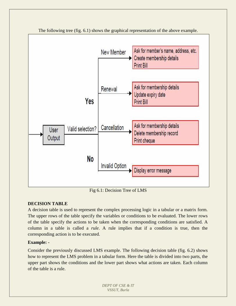
A decision tree gives a graphic view of the processing logic involved in decision making and the
corresponding actions taken. The edges of a decision tree represent conditions and the leaf nodes
represent the actions to be performed depending on the outcome of testing the condition.
Example: -
Consider Library Membership Automation Software (LMS) where it should support the
following three options:
New member
Renewal
Cancel membership
New member option-
Decision: When the 'new member' option is selected, the software asks details about the
member like the member's name, address, phone number etc.
Action: If proper information is entered then a membership record for the member is
created and a bill is printed for the annual membership charge plus the security deposit
payable.
Renewal option-
Decision: If the 'renewal' option is chosen, the LMS asks for the member's name and his
membership number to check whether he is a valid member or not.
Action: If the membership is valid then membership expiry date is updated and the
annual membership bill is printed, otherwise an error message is displayed.
Cancel membership option-
Decision: If the 'cancel membership' option is selected, then the software asks for
member's name and his membership number.
Action: The membership is cancelled, a cheque for the balance amount due to the
member is printed and finally the membership record is deleted from the database.
DEPT OF CSE & IT
VSSUT, Burla
The following tree (fig. 6.1) shows the graphical representation of the above example.
Fig 6.1: Decision Tree of LMS
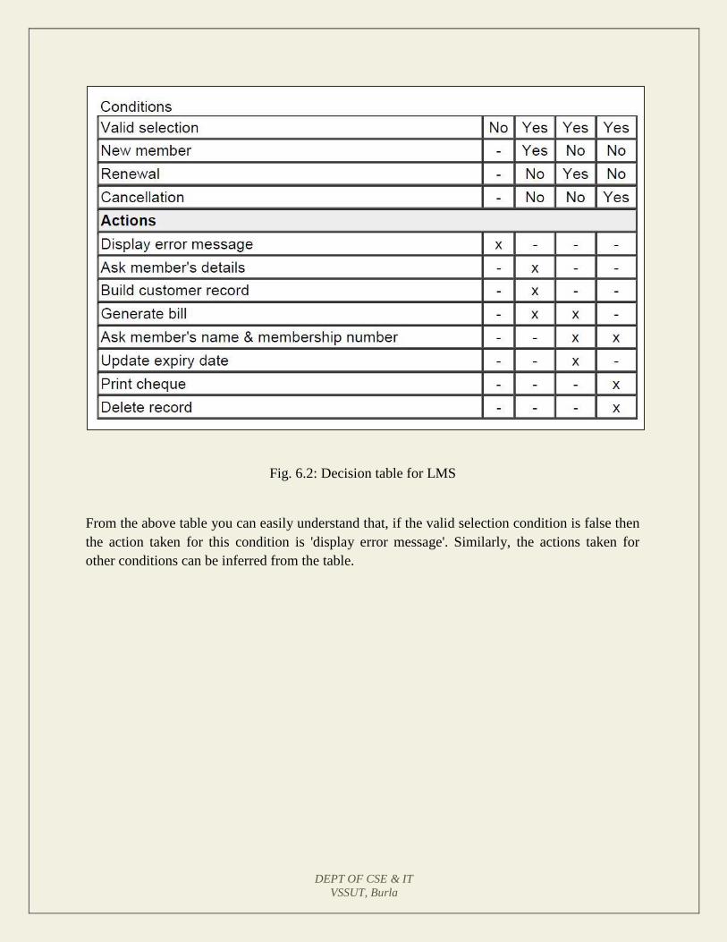
DECISION TABLE
A decision table is used to represent the complex processing logic in a tabular or a matrix form.
The upper rows of the table specify the variables or conditions to be evaluated. The lower rows
of the table specify the actions to be taken when the corresponding conditions are satisfied. A
column in a table is called a rule. A rule implies that if a condition is true, then the
corresponding action is to be executed.
Example: -
Consider the previously discussed LMS example. The following decision table (fig. 6.2) shows
how to represent the LMS problem in a tabular form. Here the table is divided into two parts, the
upper part shows the conditions and the lower part shows what actions are taken. Each column
of the table is a rule.
DEPT OF CSE & IT
VSSUT, Burla
Fig. 6.2: Decision table for LMS
From the above table you can easily understand that, if the valid selection condition is false then
the action taken for this condition is 'display error message'. Similarly, the actions taken for
other conditions can be inferred from the table.
DEPT OF CSE & IT
VSSUT, Burla
LECTURE NOTE 7
FORMAL SYSTEM SPECIFICATION
Formal Technique
A formal technique is a mathematical method to specify a hardware and/or software system,
verify whether a specification is realizable, verify that an implementation satisfies its
specification, prove properties of a system without necessarily running the system, etc. The
mathematical basis of a formal method is provided by the specification language.
Formal Specification Language
A formal specification language consists of two sets syn and sem, and a relation sat between
them. The set syn is called the syntactic domain, the set sem is called the semantic domain, and
the relation sat is called the satisfaction relation. For a given specification syn, and model of the
system sem, if sat (syn, sem), then syn is said to be the specification of sem, and sem is said to be
the specificand of syn.
Syntactic Domains
The syntactic domain of a formal specification language consists of an alphabet of symbols and
set of formation rules to construct well-formed formulas from the alphabet. The well-formed
formulas are used to specify a system.
Semantic Domains
Formal techniques can have considerably different semantic domains. Abstract data type
specification languages are used to specify algebras, theories, and programs. Programming
languages are used to specify functions from input to output values. Concurrent and distributed
system specification languages are used to specify state sequences, event sequences, state-
transition sequences, synchronization trees, partial orders, state machines, etc.
Satisfaction Relation
Given the model of a system, it is important to determine whether an element of the semantic
domain satisfies the specifications. This satisfaction is determined by using a homomorphism
known as semantic abstraction function. The semantic abstraction function maps the elements of
the semantic domain into equivalent classes. There can be different specifications describing
different aspects of a system model, possibly using different specification languages. Some of
these specifications describe the system’s behavior and the others describe the system’s
structure. Consequently, two broad classes of semantic abstraction functions are defined: those
that preserve a system’s behavior and those that preserve a system’s structure.
DEPT OF CSE & IT
VSSUT, Burla
Model-oriented vs. property-oriented approaches
Formal methods are usually classified into two broad categories – model – oriented and property
– oriented approaches. In a model-oriented style, one defines a system’s behavior directly by
constructing a model of the system in terms of mathematical structures such as tuples, relations,
functions, sets, sequences, etc.
In the property-oriented style, the system's behavior is defined indirectly by stating its properties,
usually in the form of a set of axioms that the system must satisfy.
Example:-
Let us consider a simple producer/consumer example. In a property-oriented style, it is
probably started by listing the properties of the system like: the consumer can start
consuming only after the producer has produced an item; the producer starts to produce
an item only after the consumer has consumed the last item, etc. A good example of a
producer-consumer problem is CPU-Printer coordination. After processing of data, CPU
outputs characters to the buffer for printing. Printer, on the other hand, reads characters
from the buffer and prints them. The CPU is constrained by the capacity of the buffer,
whereas the printer is constrained by an empty buffer. Examples of property-oriented
specification styles are axiomatic specification and algebraic specification.
In a model-oriented approach, we start by defining the basic operations, p (produce) and c
(consume). Then we can state that S1 + p → S, S + c → S1. Thus the model-oriented approaches
essentially specify a program by writing another, presumably simpler program. Examples of
popular model-oriented specification techniques are Z, CSP, CCS, etc.
Model-oriented approaches are more suited to use in later phases of life cycle because here even
minor changes to a specification may lead to drastic changes to the entire specification. They do
not support logical conjunctions (AND) and disjunctions (OR).
Property-oriented approaches are suitable for requirements specification because they can be
easily changed. They specify a system as a conjunction of axioms and you can easily replace one
axiom with another one.
Operational Semantics
Informally, the operational semantics of a formal method is the way computations are
represented. There are different types of operational semantics according to what is meant by a
single run of the system and how the runs are grouped together to describe the behavior of the
system. Some commonly used operational semantics are as follows:
Linear Semantics:-
In this approach, a run of a system is described by a sequence (possibly infinite) of events or
states. The concurrent activities of the system are represented by non-deterministic interleavings
of the automatic actions. For example, a concurrent activity a║b is represented by the set of
DEPT OF CSE & IT
VSSUT, Burla
sequential activities a;b and b;a. This is simple but rather unnatural representation of
concurrency. The behavior of a system in this model consists of the set of all its runs. To make
this model realistic, usually justice and fairness restrictions are imposed on computations to
exclude the unwanted interleavings.
Branching Semantics:-
In this approach, the behavior of a system is represented by a directed graph. The nodes of the
graph represent the possible states in the evolution of a system. The descendants of each node of
the graph represent the states which can be generated by any of the atomic actions enabled at that
state. Although this semantic model distinguishes the branching points in a computation, still it
represents concurrency by interleaving.
Maximally parallel semantics:-
In this approach, all the concurrent actions enabled at any state are assumed to be taken together.
This is again not a natural model of concurrency since it implicitly assumes the availability of all
the required computational resources.
Partial order semantics:-
Under this view, the semantics ascribed to a system is a structure of states satisfying a partial
order relation among the states (events). The partial order represents a precedence ordering
among events, and constraints some events to occur only after some other events have occurred;
while the occurrence of other events (called concurrent events) is considered to be incomparable.
This fact identifies concurrency as a phenomenon not translatable to any interleaved
representation.
Formal methods possess several positive features, some of which are discussed below.
Formal specifications encourage rigor. Often, the very process of construction of a
rigorous specification is more important than the formal specification itself. The
construction of a rigorous specification clarifies several aspects of system behavior
that are not obvious in an informal specification.
Formal methods usually have a well-founded mathematical basis. Thus, formal
specifications are not only more precise, but also mathematically sound and can be
used to reason about the properties of a specification and to rigorously prove that an
implementation satisfies its specifications.
Formal methods have well-defined semantics. Therefore, ambiguity in specifications
is automatically avoided when one formally specifies a system.
DEPT OF CSE & IT
VSSUT, Burla
The mathematical basis of the formal methods facilitates automating the analysis of
specifications. For example, a tableau-based technique has been used to automatically
check the consistency of specifications. Also, automatic theorem proving techniques
can be used to verify that an implementation satisfies its specifications. The
possibility of automatic verification is one of the most important advantages of formal
methods.
Formal specifications can be executed to obtain immediate feedback on the features
of the specified system. This concept of executable specifications is related to rapid
prototyping. Informally, a prototype is a “toy” working model of a system that can
provide immediate feedback on the behavior of the specified system, and is especially
useful in checking the completeness of specifications.
Limitations of formal requirements specification
It is clear that formal methods provide mathematically sound frameworks within large, complex
systems can be specified, developed and verified in a systematic rather than in an ad hoc manner.
However, formal methods suffer from several shortcomings, some of which are the following:
Formal methods are difficult to learn and use.
The basic incompleteness results of first-order logic suggest that it is impossible to
check absolute correctness of systems using theorem proving techniques.
Formal techniques are not able to handle complex problems. This shortcoming results
from the fact that, even moderately complicated problems blow up the complexity of
formal specification and their analysis. Also, a large unstructured set of mathematical
formulas is difficult to comprehend.
Axiomatic Specification
In axiomatic specification of a system, first-order logic is used to write the pre and post-
conditions to specify the operations of the system in the form of axioms. The pre-conditions
basically capture the conditions that must be satisfied before an operation can successfully be
invoked. In essence, the pre-conditions capture the requirements on the input parameters of a
function. The post-conditions are the conditions that must be satisfied when a function completes
execution for the function to be considered to have executed successfully. Thus, the post-
conditions are essentially constraints on the results produced for the function execution to be
considered successful.
DEPT OF CSE & IT
VSSUT, Burla
The following are the sequence of steps that can be followed to systematically develop the
axiomatic specifications of a function:
Establish the range of input values over which the function should behave correctly.
Also find out other constraints on the input parameters and write it in the form of a
predicate.
Specify a predicate defining the conditions which must hold on the output of the
function if it behaved properly.
Establish the changes made to the function’s input parameters after execution of the
function. Pure mathematical functions do not change their input and therefore this
type of assertion is not necessary for pure functions.
Combine all of the above into pre and post conditions of the function.
Example1: -
Specify the pre- and post-conditions of a function that takes a real number as argument
and returns half the input value if the input is less than or equal to 100, or else returns
double the value.
f (x : real) : real
pre : x ∈ R
post : {(x≤100) ∧ (f(x) = x/2)} ∨ {(x>100) ∧ (f(x) = 2∗x)}
Example2: -
Axiomatically specify a function named search which takes an integer array and an
integer key value as its arguments and returns the index in the array where the key value
is present.
search(X : IntArray, key : Integer) : Integer
pre : ∃ i ∈ [Xfirst….Xlast], X[i] = key
post : {(X′[search(X, key)] = key) ∧ (X = X′)}
Here the convention followed is: If a function changes any of its input parameters and if
that parameter is named X, and then it is referred to as X′ after the function completes
execution faster.
DEPT OF CSE & IT
VSSUT, Burla
LECTURE NOTE 8
SOFTWARE DESIGN Software design is a process to transform user requirements into some suitable form, which
helps the programmer in software coding and implementation.
For assessing user requirements, an SRS (Software Requirement Specification) document is
created whereas for coding and implementation, there is a need of more specific and detailed
requirements in software terms. The output of this process can directly be used into
implementation in programming languages.
Software design is the first step in SDLC (Software Design Life Cycle), which moves the
concentration from problem domain to solution domain. It tries to specify how to fulfill the
requirements mentioned in SRS.
Software Design Levels
Software design yields three levels of results:
Architectural Design - The architectural design is the highest abstract version of the
system. It identifies the software as a system with many components interacting with
each other. At this level, the designers get the idea of proposed solution domain.
High-level Design- The high-level design breaks the ‘single entity-multiple component’
concept of architectural design into less-abstracted view of sub-systems and modules and
depicts their interaction with each other. High-level design focuses on how the system
along with all of its components can be implemented in forms of modules. It recognizes
modular structure of each sub-system and their relation and interaction among each other.
Detailed Design- Detailed design deals with the implementation part of what is seen as a
system and its sub-systems in the previous two designs. It is more detailed towards
modules and their implementations. It defines logical structure of each module and their
interfaces to communicate with other modules.
Modularization
Modularization is a technique to divide a software system into multiple discrete and
independent modules, which are expected to be capable of carrying out task(s) independently.
These modules may work as basic constructs for the entire software. Designers tend to design
modules such that they can be executed and/or compiled separately and independently.
Modular design unintentionally follows the rules of ‘divide and conquer’ problem-solving
strategy this is because there are many other benefits attached with the modular design of a
software.
DEPT OF CSE & IT
VSSUT, Burla
Advantage of modularization:
Smaller components are easier to maintain
Program can be divided based on functional aspects
Desired level of abstraction ca n be brought in the program
Components with high cohesion can be re-used again.
Concurrent execution can be made possible
Desired from security aspect
Concurrency
Back in time, all softwares were meant to be executed sequentially. By sequential execution we
mean that the coded instruction will be executed one after another implying only one portion of
program being activated at any given time. Say, a software has multiple modules, then only one
of all the modules can be found active at any time of execution.
In software design, concurrency is implemented by splitting the software into multiple
independent units of execution, like modules and executing them in parallel. In other words,
concurrency provides capability to the software to execute more than one part of code in
parallel to each other.
It is necessary for the programmers and designers to recognize those modules, which can be
made parallel execution.
Example
The spell check feature in word processor is a module of software, which runs alongside the
word processor itself.
Coupling and Cohesion
When a software program is modularized, its tasks are divided into several modules based on
some characteristics. As we know, modules are set of instructions put together in order to
achieve some tasks. They are though, considered as single entity but may refer to each other to
work together. There are measures by which the quality of a design of modules and their
interaction among them can be measured. These measures are called coupling and cohesion.
Cohesion
Cohesion is a measure that defines the degree of intra-dependability within elements of a
module. The greater the cohesion, the better is the program design.
DEPT OF CSE & IT
VSSUT, Burla
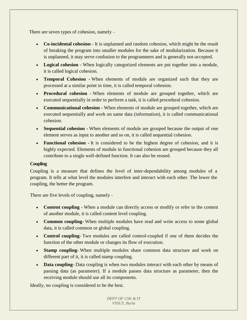
There are seven types of cohesion, namely –
Co-incidental cohesion - It is unplanned and random cohesion, which might be the result
of breaking the program into smaller modules for the sake of modularization. Because it
is unplanned, it may serve confusion to the programmers and is generally not-accepted.
Logical cohesion - When logically categorized elements are put together into a module,
it is called logical cohesion.
Temporal Cohesion - When elements of module are organized such that they are
processed at a similar point in time, it is called temporal cohesion.
Procedural cohesion - When elements of module are grouped together, which are
executed sequentially in order to perform a task, it is called procedural cohesion.
Communicational cohesion - When elements of module are grouped together, which are
executed sequentially and work on same data (information), it is called communicational
cohesion.
Sequential cohesion - When elements of module are grouped because the output of one
element serves as input to another and so on, it is called sequential cohesion.
Functional cohesion - It is considered to be the highest degree of cohesion, and it is
highly expected. Elements of module in functional cohesion are grouped because they all
contribute to a single well-defined function. It can also be reused.
Coupling
Coupling is a measure that defines the level of inter-dependability among modules of a
program. It tells at what level the modules interfere and interact with each other. The lower the
coupling, the better the program.
There are five levels of coupling, namely -
Content coupling - When a module can directly access or modify or refer to the content
of another module, it is called content level coupling.
Common coupling- When multiple modules have read and write access to some global
data, it is called common or global coupling.
Control coupling- Two modules are called control-coupled if one of them decides the
function of the other module or changes its flow of execution.
Stamp coupling- When multiple modules share common data structure and work on
different part of it, it is called stamp coupling.
Data coupling- Data coupling is when two modules interact with each other by means of
passing data (as parameter). If a module passes data structure as parameter, then the
receiving module should use all its components.
Ideally, no coupling is considered to be the best.
DEPT OF CSE & IT
VSSUT, Burla
Design Verification
The output of software design process is design documentation, pseudo codes, detailed logic
diagrams, process diagrams, and detailed description of all functional or non-functional
requirements.
The next phase, which is the implementation of software, depends on all outputs mentioned
above.
It is then becomes necessary to verify the output before proceeding to the next phase. The early
any mistake is detected, the better it is or it might not be detected until testing of the product. If
the outputs of design phase are in formal notation form, then their associated tools for
verification should be used otherwise a thorough design review can be used for verification and
validation.
By structured verification approach, reviewers can detect defects that might be caused by
overlooking some conditions. A good design review is important for good software design,
accuracy and quality.
DEPT OF CSE & IT
VSSUT, Burla
LECTURE NOTE 9
SOFTWARE DESIGN STRATEGIES
Software design is a process to conceptualize the software requirements into software
implementation. Software design takes the user requirements as challenges and tries to find
optimum solution. While the software is being conceptualized, a plan is chalked out to find the
best possible design for implementing the intended solution.
There are multiple variants of software design. Let us study them briefly:
Structured Design
Structured design is a conceptualization of problem into several well-organized elements of
solution. It is basically concerned with the solution design. Benefit of structured design is, it
gives better understanding of how the problem is being solved. Structured design also makes it
simpler for designer to concentrate on the problem more accurately.
Structured design is mostly based on ‘divide and conquer’ strategy where a problem is broken
into several small problems and each small problem is individually solved until the whole
problem is solved.
The small pieces of problem are solved by means of solution modules. Structured design
emphasis that these modules be well organized in order to achieve precise solution.
These modules are arranged in hierarchy. They communicate with each other. A good structured
design always follows some rules for communication among multiple modules, namely -
Cohesion - grouping of all functionally related elements.
Coupling - communication between different modules.
A good structured design has high cohesion and low coupling arrangements.
DEPT OF CSE & IT
VSSUT, Burla
Function Oriented Design
In function-oriented design, the system is comprised of many smaller sub-systems known as
functions. These functions are capable of performing significant task in the system. The system
is considered as top view of all functions.
Function oriented design inherits some properties of structured design where divide and conquer
methodology is used.
This design mechanism divides the whole system into smaller functions, which provides means
of abstraction by concealing the information and their operation. These functional modules can
share information among themselves by means of information passing and using information
available globally.
Another characteristic of functions is that when a program calls a function, the function changes
the state of the program, which sometimes is not acceptable by other modules. Function oriented
design works well where the system state does not matter and program/functions work on input
rather than on a state.
Design Process
The whole system is seen as how data flows in the system by means of data flow
diagram.
DFD depicts how functions change the data and state of entire system.
The entire system is logically broken down into smaller units known as functions on the
basis of their operation in the system.
Each function is then described at large.
Object Oriented Design
Object oriented design works around the entities and their characteristics instead of functions
involved in the software system. This design strategy focuses on entities and its characteristics.
The whole concept of software solution revolves around the engaged entities.
Let us see the important concepts of Object Oriented Design:
Objects - All entities involved in the solution design are known as objects. For example,
person, banks, company and customers are treated as objects. Every entity has some
attributes associated to it and has some methods to perform on the attributes.
Classes - A class is a generalized description of an object. An object is an instance of a
class. Class defines all the attributes, which an object can have and methods, which
defines the functionality of the object.

DEPT OF CSE & IT
VSSUT, Burla
In the solution design, attributes are stored as variables and functionalities are defined
by means of methods or procedures.
Encapsulation - In OOD, the attributes (data variables) and methods (operation on the
data) are bundled together is called encapsulation. Encapsulation not only bundles
important information of an object together, but also restricts access of the data and
methods from the outside world. This is called information hiding.
Inheritance - OOD allows similar classes to stack up in hierarchical manner where the
lower or sub-classes can import, implement and re-use allowed variables and methods
from their immediate super classes. This property of OOD is known as inheritance. This
makes it easier to define specific class and to create generalized classes from specific
ones.
Polymorphism - OOD languages provide a mechanism where methods performing
similar tasks but vary in arguments, can be assigned same name. This is called
polymorphism, which allows a single interface performing tasks for different types.
Depending upon how the function is invoked, respective portion of the code gets
executed.
Design Process
Software design process can be perceived as series of well-defined steps. Though it varies
according to design approach (function oriented or object oriented, yet It may have the
following steps involved:
A solution design is created from requirement or previous used system and/or system
sequence diagram.
Objects are identified and grouped into classes on behalf of similarity in attribute
characteristics.
Class hierarchy and relation among them are defined.
Application framework is defined.
Software Design Approaches
There are two generic approaches for software designing:
Top down Design
We know that a system is composed of more than one sub-systems and it contains a number of
components. Further, these sub-systems and components may have their one set of sub-system
and components and creates hierarchical structure in the system.
Top-down design takes the whole software system as one entity and then decomposes it to
achieve more than one sub-system or component based on some characteristics. Each sub-
DEPT OF CSE & IT
VSSUT, Burla
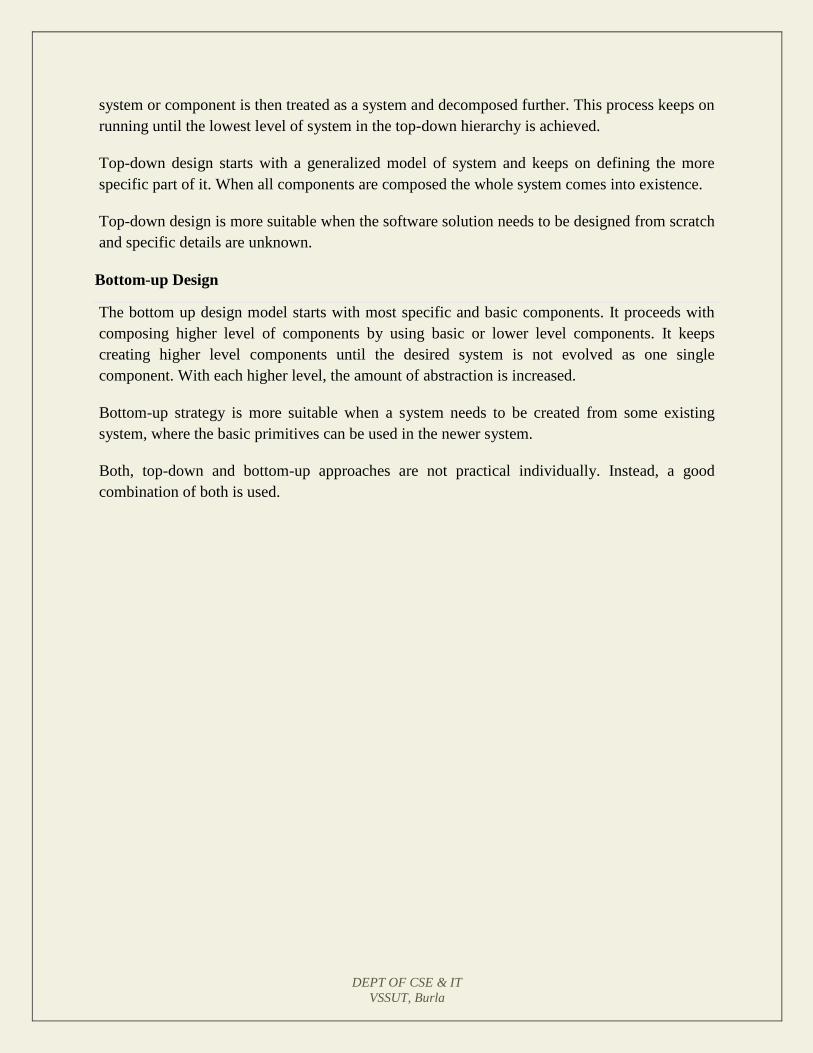
system or component is then treated as a system and decomposed further. This process keeps on
running until the lowest level of system in the top-down hierarchy is achieved.
Top-down design starts with a generalized model of system and keeps on defining the more
specific part of it. When all components are composed the whole system comes into existence.
Top-down design is more suitable when the software solution needs to be designed from scratch
and specific details are unknown.
Bottom-up Design
The bottom up design model starts with most specific and basic components. It proceeds with
composing higher level of components by using basic or lower level components. It keeps
creating higher level components until the desired system is not evolved as one single
component. With each higher level, the amount of abstraction is increased.
Bottom-up strategy is more suitable when a system needs to be created from some existing
system, where the basic primitives can be used in the newer system.
Both, top-down and bottom-up approaches are not practical individually. Instead, a good
combination of both is used.
DEPT OF CSE & IT
VSSUT, Burla
LECTURE NOTE 10
SOFTWARE ANALYSIS & DESIGN TOOLS
Software analysis and design includes all activities, which help the transformation of
requirement specification into implementation. Requirement specifications specify all functional
and non-functional expectations from the software. These requirement specifications come in
the shape of human readable and understandable documents, to which a computer has nothing to
do.
Software analysis and design is the intermediate stage, which helps human-readable
requirements to be transformed into actual code.
Let us see few analysis and design tools used by software designers:
Data Flow Diagram
Data flow diagram is a graphical representation of data flow in an information system. It is
capable of depicting incoming data flow, outgoing data flow and stored data. The DFD does not
mention anything about how data flows through the system.
There is a prominent difference between DFD and Flowchart. The flowchart depicts flow of
control in program modules. DFDs depict flow of data in the system at various levels. DFD does
not contain any control or branch elements.
Types of DFD
Data Flow Diagrams are either Logical or Physical.
Logical DFD - This type of DFD concentrates on the system process and flow of data in
the system. For example in a Banking software system, how data is moved between
different entities.
Physical DFD - This type of DFD shows how the data flow is actually implemented in
the system. It is more specific and close to the implementation.

DEPT OF CSE & IT
VSSUT, Burla
DFD Components
DFD can represent Source, destination, storage and flow of data using the following set of
components -
Fig 10.1: DFD Components
Entities - Entities are source and destination of information data. Entities are represented
by rectangles with their respective names.
Process - Activities and action taken on the data are represented by Circle or Round-
edged rectangles.
Data Storage - There are two variants of data storage - it can either be represented as a
rectangle with absence of both smaller sides or as an open-sided rectangle with only one
side missing.
Data Flow - Movement of data is shown by pointed arrows. Data movement is shown
from the base of arrow as its source towards head of the arrow as destination.
Importance of DFDs in a good software design
The main reason why the DFD technique is so popular is probably because of the fact that DFD
is a very simple formalism – it is simple to understand and use. Starting with a set of high-level
functions that a system performs, a DFD model hierarchically represents various sub-functions.
In fact, any hierarchical model is simple to understand. Human mind is such that it can easily
understand any hierarchical model of a system – because in a hierarchical model, starting with a
very simple and abstract model of a system, different details of the system are slowly introduced
through different hierarchies. The data flow diagramming technique also follows a very simple
set of intuitive concepts and rules. DFD is an elegant modeling technique that turns out to be
useful not only to represent the results of structured analysis of a software problem, but also for
several other applications such as showing the flow of documents or items in an organization.
DEPT OF CSE & IT
VSSUT, Burla
Data Dictionary
A data dictionary lists all data items appearing in the DFD model of a system. The data items
listed include all data flows and the contents of all data stores appearing on the DFDs in the DFD
model of a system. A data dictionary lists the purpose of all data items and the definition of all
composite data items in terms of their component data items. For example, a data dictionary
entry may represent that the data grossPay consists of the components regularPay and
overtimePay.
grossPay = regularPay + overtimePay
For the smallest units of data items, the data dictionary lists their name and their type. Composite
data items can be defined in terms of primitive data items using the following data definition
operators:
+: denotes composition of two data items, e.g. a+b represents data a and b.
[,,]: represents selection, i.e. any one of the data items listed in the brackets can occur.
For example, [a,b] represents either a occurs or b occurs.
(): the contents inside the bracket represent optional data which may or may not appear.
e.g. a+(b) represents either a occurs or a+b occurs.
{}: represents iterative data definition, e.g. {name}5 represents five name data. {name}*
represents zero or more instances of name data.
=: represents equivalence, e.g. a=b+c means that a represents b and c.
/* */: Anything appearing within /* and */ is considered as a comment.
Example 1: Tic-Tac-Toe Computer Game
Tic-tac-toe is a computer game in which a human player and the computer make
alternative moves on a 3×3 square. A move consists of marking previously
unmarked square. The player who first places three consecutive marks along a
straight line on the square (i.e. along a row, column, or diagonal) wins the game.
As soon as either the human player or the computer wins, a message
congratulating the winner should be displayed. If neither player manages to get
three consecutive marks along a straight line, but all the squares on the board are
filled up, then the game is drawn. The computer always tries to win a game.
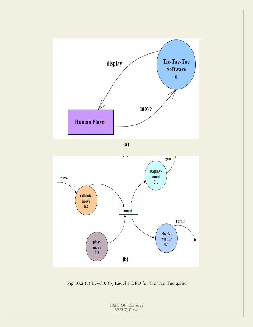
DEPT OF CSE & IT
VSSUT, Burla
(a)
Fig 10.2 (a) Level 0 (b) Level 1 DFD for Tic-Tac-Toe game
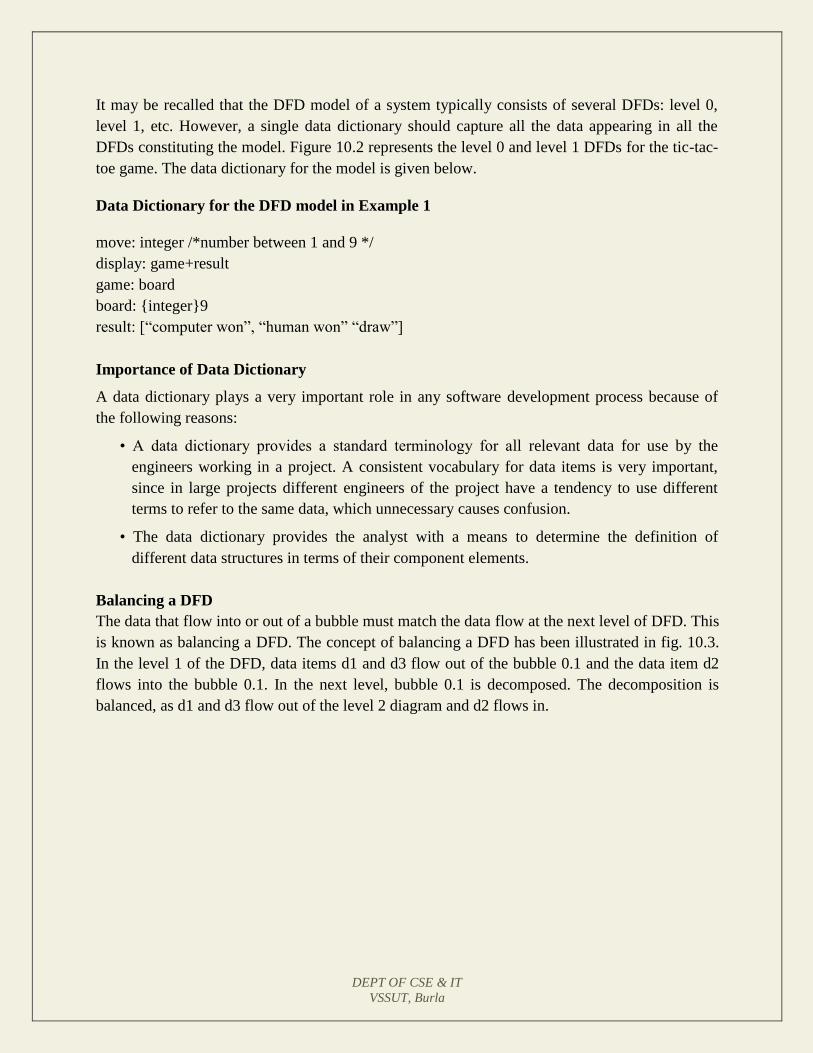
DEPT OF CSE & IT
VSSUT, Burla
It may be recalled that the DFD model of a system typically consists of several DFDs: level 0,
level 1, etc. However, a single data dictionary should capture all the data appearing in all the
DFDs constituting the model. Figure 10.2 represents the level 0 and level 1 DFDs for the tic-tac-
toe game. The data dictionary for the model is given below.
Data Dictionary for the DFD model in Example 1
move: integer /*number between 1 and 9 */
display: game+result
game: board
board: {integer}9
result: [“computer won”, “human won” “draw”]
Importance of Data Dictionary
A data dictionary plays a very important role in any software development process because of
the following reasons:
• A data dictionary provides a standard terminology for all relevant data for use by the
engineers working in a project. A consistent vocabulary for data items is very important,
since in large projects different engineers of the project have a tendency to use different
terms to refer to the same data, which unnecessary causes confusion.
• The data dictionary provides the analyst with a means to determine the definition of
different data structures in terms of their component elements.
Balancing a DFD
The data that flow into or out of a bubble must match the data flow at the next level of DFD. This
is known as balancing a DFD. The concept of balancing a DFD has been illustrated in fig. 10.3.
In the level 1 of the DFD, data items d1 and d3 flow out of the bubble 0.1 and the data item d2
flows into the bubble 0.1. In the next level, bubble 0.1 is decomposed. The decomposition is
balanced, as d1 and d3 flow out of the level 2 diagram and d2 flows in.
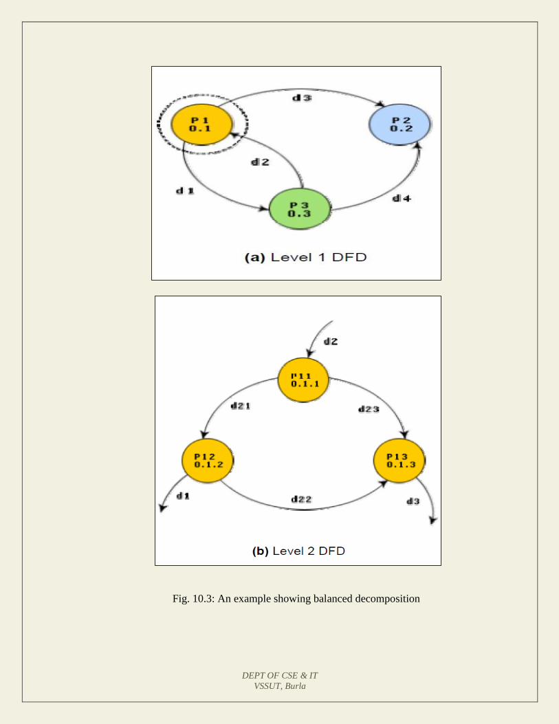
DEPT OF CSE & IT
VSSUT, Burla
Fig. 10.3: An example showing balanced decomposition
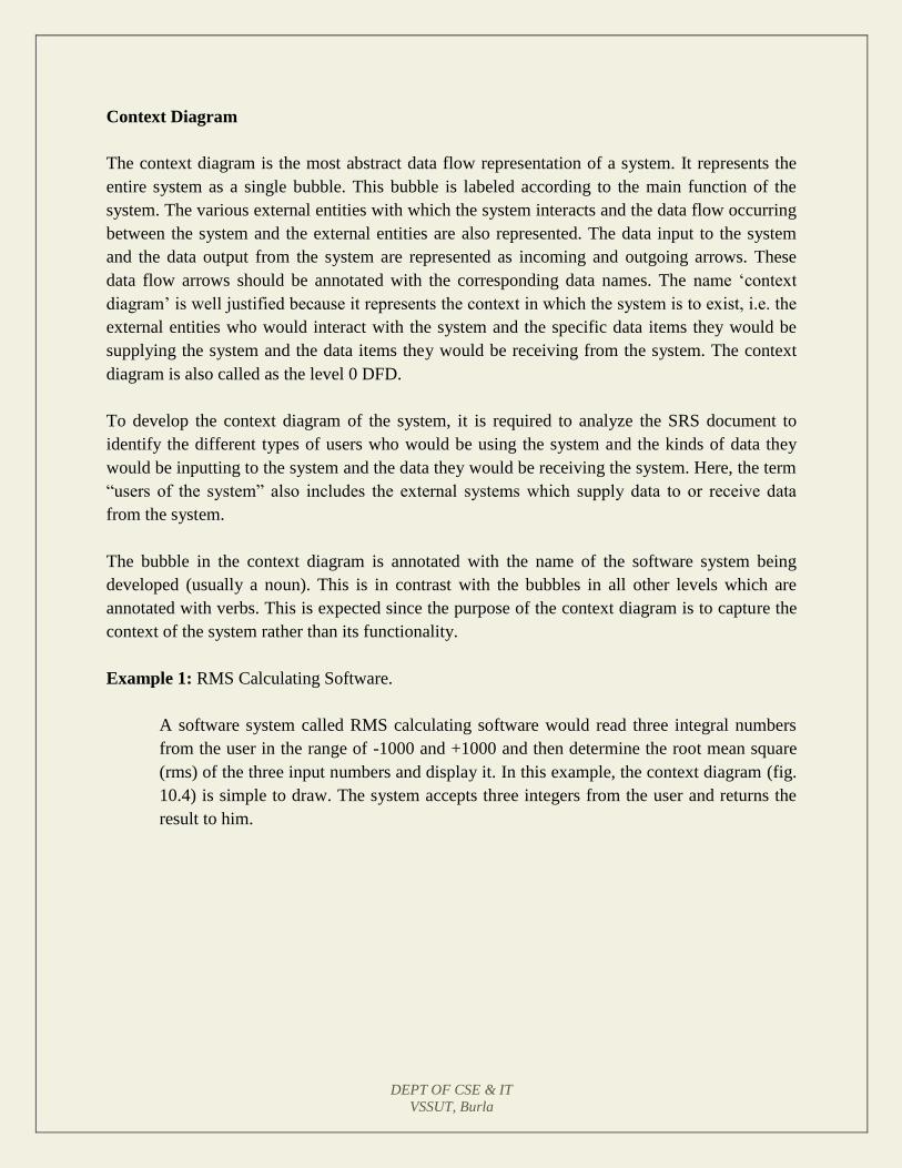
DEPT OF CSE & IT
VSSUT, Burla
Context Diagram
The context diagram is the most abstract data flow representation of a system. It represents the
entire system as a single bubble. This bubble is labeled according to the main function of the
system. The various external entities with which the system interacts and the data flow occurring
between the system and the external entities are also represented. The data input to the system
and the data output from the system are represented as incoming and outgoing arrows. These
data flow arrows should be annotated with the corresponding data names. The name ‘context
diagram’ is well justified because it represents the context in which the system is to exist, i.e. the
external entities who would interact with the system and the specific data items they would be
supplying the system and the data items they would be receiving from the system. The context
diagram is also called as the level 0 DFD.
To develop the context diagram of the system, it is required to analyze the SRS document to
identify the different types of users who would be using the system and the kinds of data they
would be inputting to the system and the data they would be receiving the system. Here, the term
“users of the system” also includes the external systems which supply data to or receive data
from the system.
The bubble in the context diagram is annotated with the name of the software system being
developed (usually a noun). This is in contrast with the bubbles in all other levels which are
annotated with verbs. This is expected since the purpose of the context diagram is to capture the
context of the system rather than its functionality.
Example 1: RMS Calculating Software.
A software system called RMS calculating software would read three integral numbers
from the user in the range of -1000 and +1000 and then determine the root mean square
(rms) of the three input numbers and display it. In this example, the context diagram (fig.
10.4) is simple to draw. The system accepts three integers from the user and returns the
result to him.
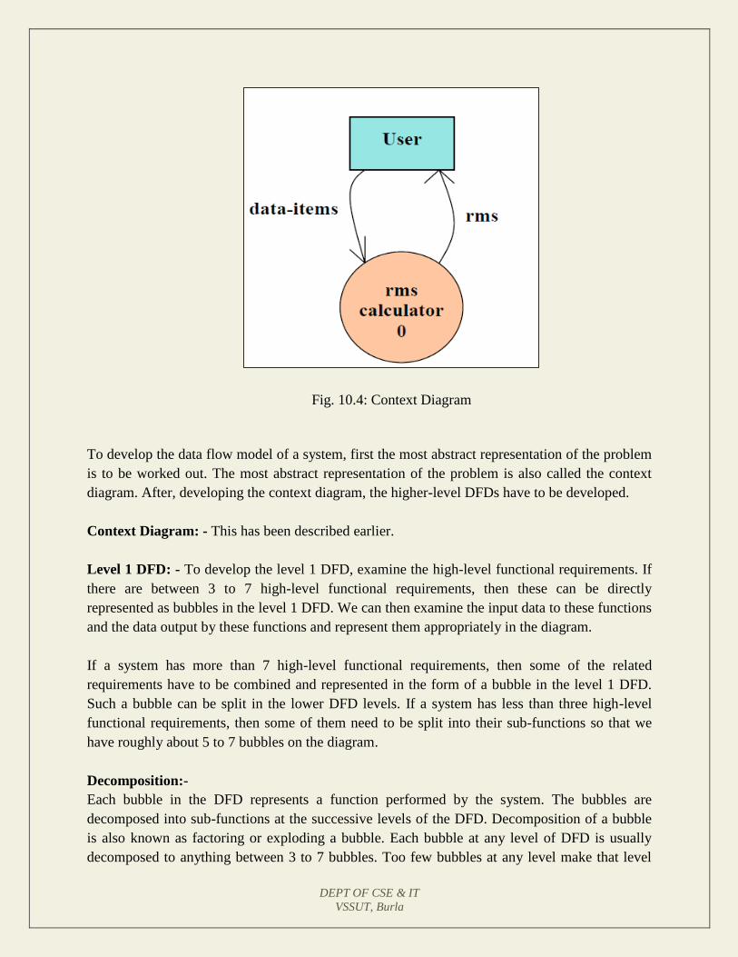
DEPT OF CSE & IT
VSSUT, Burla
Fig. 10.4: Context Diagram
To develop the data flow model of a system, first the most abstract representation of the problem
is to be worked out. The most abstract representation of the problem is also called the context
diagram. After, developing the context diagram, the higher-level DFDs have to be developed.
Context Diagram: - This has been described earlier.
Level 1 DFD: - To develop the level 1 DFD, examine the high-level functional requirements. If
there are between 3 to 7 high-level functional requirements, then these can be directly
represented as bubbles in the level 1 DFD. We can then examine the input data to these functions
and the data output by these functions and represent them appropriately in the diagram.
If a system has more than 7 high-level functional requirements, then some of the related
requirements have to be combined and represented in the form of a bubble in the level 1 DFD.
Such a bubble can be split in the lower DFD levels. If a system has less than three high-level
functional requirements, then some of them need to be split into their sub-functions so that we
have roughly about 5 to 7 bubbles on the diagram.
Decomposition:-
Each bubble in the DFD represents a function performed by the system. The bubbles are
decomposed into sub-functions at the successive levels of the DFD. Decomposition of a bubble
is also known as factoring or exploding a bubble. Each bubble at any level of DFD is usually
decomposed to anything between 3 to 7 bubbles. Too few bubbles at any level make that level
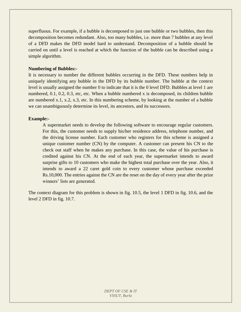
DEPT OF CSE & IT
VSSUT, Burla
superfluous. For example, if a bubble is decomposed to just one bubble or two bubbles, then this
decomposition becomes redundant. Also, too many bubbles, i.e. more than 7 bubbles at any level
of a DFD makes the DFD model hard to understand. Decomposition of a bubble should be
carried on until a level is reached at which the function of the bubble can be described using a
simple algorithm.
Numbering of Bubbles:-
It is necessary to number the different bubbles occurring in the DFD. These numbers help in
uniquely identifying any bubble in the DFD by its bubble number. The bubble at the context
level is usually assigned the number 0 to indicate that it is the 0 level DFD. Bubbles at level 1 are
numbered, 0.1, 0.2, 0.3, etc, etc. When a bubble numbered x is decomposed, its children bubble
are numbered x.1, x.2, x.3, etc. In this numbering scheme, by looking at the number of a bubble
we can unambiguously determine its level, its ancestors, and its successors.
Example:-
A supermarket needs to develop the following software to encourage regular customers.
For this, the customer needs to supply his/her residence address, telephone number, and
the driving license number. Each customer who registers for this scheme is assigned a
unique customer number (CN) by the computer. A customer can present his CN to the
check out staff when he makes any purchase. In this case, the value of his purchase is
credited against his CN. At the end of each year, the supermarket intends to award
surprise gifts to 10 customers who make the highest total purchase over the year. Also, it
intends to award a 22 caret gold coin to every customer whose purchase exceeded
Rs.10,000. The entries against the CN are the reset on the day of every year after the prize
winners’ lists are generated.
The context diagram for this problem is shown in fig. 10.5, the level 1 DFD in fig. 10.6, and the
level 2 DFD in fig. 10.7.

DEPT OF CSE & IT
VSSUT, Burla
Fig. 10.5: Context diagram for supermarket problem
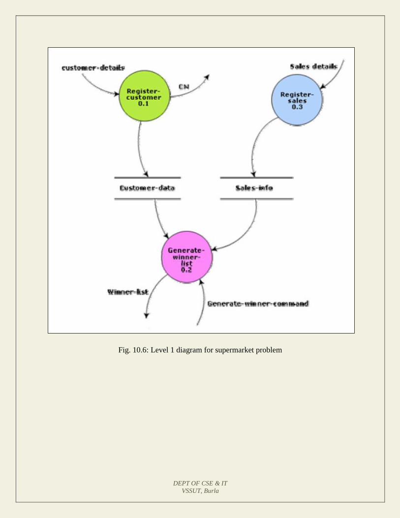
DEPT OF CSE & IT
VSSUT, Burla
Fig. 10.6: Level 1 diagram for supermarket problem
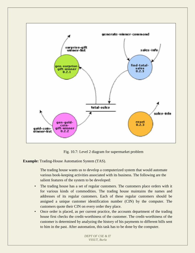
DEPT OF CSE & IT
VSSUT, Burla
Fig. 10.7: Level 2 diagram for supermarket problem
Example: Trading-House Automation System (TAS).
The trading house wants us to develop a computerized system that would automate
various book-keeping activities associated with its business. The following are the
salient features of the system to be developed:
• The trading house has a set of regular customers. The customers place orders with it
for various kinds of commodities. The trading house maintains the names and
addresses of its regular customers. Each of these regular customers should be
assigned a unique customer identification number (CIN) by the computer. The
customers quote their CIN on every order they place.
• Once order is placed, as per current practice, the accounts department of the trading
house first checks the credit-worthiness of the customer. The credit-worthiness of the
customer is determined by analyzing the history of his payments to different bills sent
to him in the past. After automation, this task has to be done by the computer.
DEPT OF CSE & IT
VSSUT, Burla
• If the customer is not credit-worthy, his orders are not processed any further and an
appropriate order rejection message is generated for the customer.
• If a customer is credit-worthy, the items that have been ordered are checked against a
list of items that the trading house deals with. The items in the order which the
trading house does not deal with, are not processed any further and an appropriate
apology message for the customer for these items is generated.
• The items in the customer’s order that the trading house deals with are checked for
availability in the inventory. If the items are available in the inventory in the desired
quantity, then
A bill with the forwarding address of the customer is printed.
A material issue slip is printed. The customer can produce this material
issue slip at the store house and take delivery of the items.
Inventory data is adjusted to reflect the sale to the customer.
If any of the ordered items are not available in the inventory in sufficient quantity to
satisfy the order, then these out-of-stock items along with the quantity ordered by the
customer and the CIN are stored in a “pending-order” file for the further processing to
be carried out when the purchase department issues the “generate indent” command.
• The purchase department should be allowed to periodically issue commands to
generate indents. When a command to generate indents is issued, the system should
examine the “pending-order” file to determine the orders that are pending and
determine the total quantity required for each of the items. It should find out the
addresses of the vendors who supply these items by examining a file containing
vendor details and then should print out indents to these vendors.
• The system should also answer managerial queries regarding the statistics of different
items sold over any given period of time and the corresponding quantity sold and the
price realized.
The context diagram for the trading house automation problem is shown in fig. 10.8, and
the level 1 DFD in fig. 10.9.
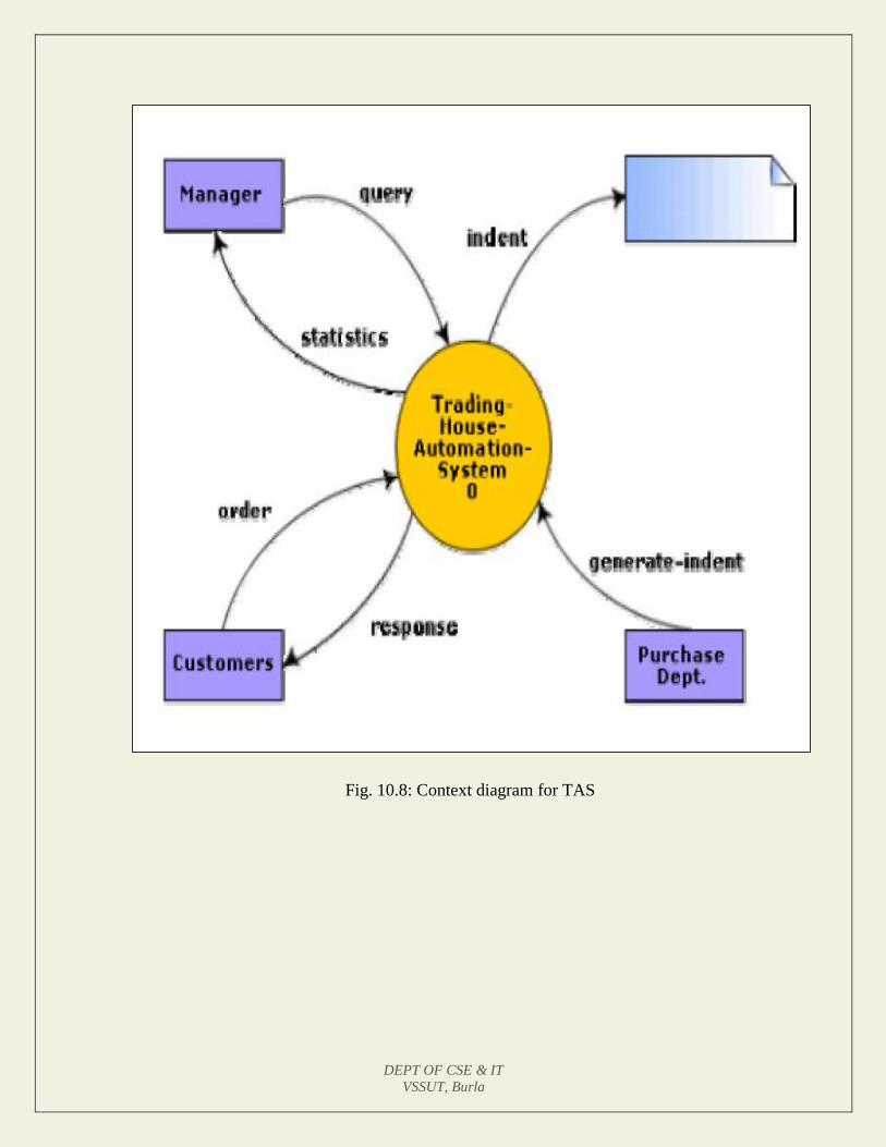
DEPT OF CSE & IT
VSSUT, Burla
Fig. 10.8: Context diagram for TAS
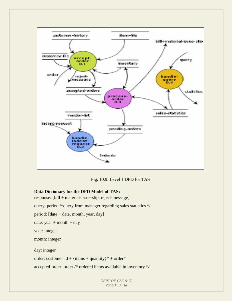
DEPT OF CSE & IT
VSSUT, Burla
Fig. 10.9: Level 1 DFD for TAS
Data Dictionary for the DFD Model of TAS:
response: [bill + material-issue-slip, reject-message]
query: period /*query from manager regarding sales statistics */
period: [date + date, month, year, day]
date: year + month + day
year: integer
month: integer
day: integer
order: customer-id + {items + quantity}* + order#
accepted-order: order /* ordered items available in inventory */
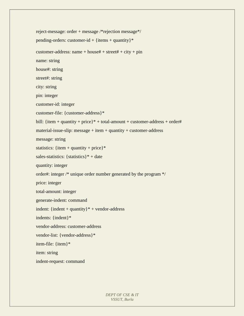
DEPT OF CSE & IT
VSSUT, Burla
reject-message: order + message /*rejection message*/
pending-orders: customer-id + {items + quantity}*
customer-address: name + house# + street# + city + pin
name: string
house#: string
street#: string
city: string
pin: integer
customer-id: integer
customer-file: {customer-address}*
bill: {item + quantity + price}* + total-amount + customer-address + order#
material-issue-slip: message + item + quantity + customer-address
message: string
statistics: {item + quantity + price}*
sales-statistics: {statistics}* + date
quantity: integer
order#: integer /* unique order number generated by the program */
price: integer
total-amount: integer
generate-indent: command
indent: {indent + quantity}* + vendor-address
indents: {indent}*
vendor-address: customer-address
vendor-list: {vendor-address}*
item-file: {item}*
item: string
indent-request: command
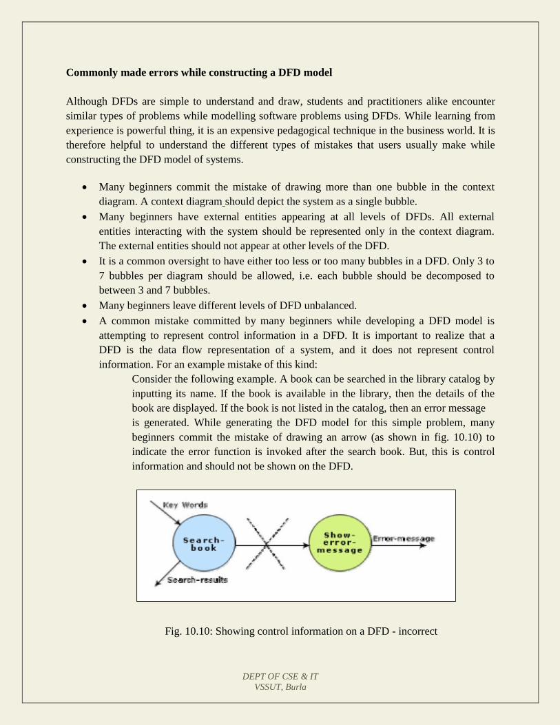
DEPT OF CSE & IT
VSSUT, Burla
Commonly made errors while constructing a DFD model
Although DFDs are simple to understand and draw, students and practitioners alike encounter
similar types of problems while modelling software problems using DFDs. While learning from
experience is powerful thing, it is an expensive pedagogical technique in the business world. It is
therefore helpful to understand the different types of mistakes that users usually make while
constructing the DFD model of systems.
Many beginners commit the mistake of drawing more than one bubble in the context
diagram. A context diagram should depict the system as a single bubble.
Many beginners have external entities appearing at all levels of DFDs. All external
entities interacting with the system should be represented only in the context diagram.
The external entities should not appear at other levels of the DFD.
It is a common oversight to have either too less or too many bubbles in a DFD. Only 3 to
7 bubbles per diagram should be allowed, i.e. each bubble should be decomposed to
between 3 and 7 bubbles.
Many beginners leave different levels of DFD unbalanced.
A common mistake committed by many beginners while developing a DFD model is
attempting to represent control information in a DFD. It is important to realize that a
DFD is the data flow representation of a system, and it does not represent control
information. For an example mistake of this kind:
Consider the following example. A book can be searched in the library catalog by
inputting its name. If the book is available in the library, then the details of the
book are displayed. If the book is not listed in the catalog, then an error message
is generated. While generating the DFD model for this simple problem, many
beginners commit the mistake of drawing an arrow (as shown in fig. 10.10) to
indicate the error function is invoked after the search book. But, this is control
information and should not be shown on the DFD.
Fig. 10.10: Showing control information on a DFD - incorrect
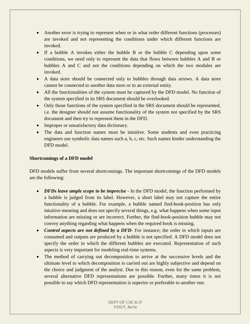
DEPT OF CSE & IT
VSSUT, Burla
Another error is trying to represent when or in what order different functions (processes)
are invoked and not representing the conditions under which different functions are
invoked.
If a bubble A invokes either the bubble B or the bubble C depending upon some
conditions, we need only to represent the data that flows between bubbles A and B or
bubbles A and C and not the conditions depending on which the two modules are
invoked.
A data store should be connected only to bubbles through data arrows. A data store
cannot be connected to another data store or to an external entity.
All the functionalities of the system must be captured by the DFD model. No function of
the system specified in its SRS document should be overlooked.
Only those functions of the system specified in the SRS document should be represented,
i.e. the designer should not assume functionality of the system not specified by the SRS
document and then try to represent them in the DFD.
Improper or unsatisfactory data dictionary.
The data and function names must be intuitive. Some students and even practicing
engineers use symbolic data names such a, b, c, etc. Such names hinder understanding the
DFD model.
Shortcomings of a DFD model
DFD models suffer from several shortcomings. The important shortcomings of the DFD models
are the following:
DFDs leave ample scope to be imprecise - In the DFD model, the function performed by
a bubble is judged from its label. However, a short label may not capture the entire
functionality of a bubble. For example, a bubble named find-book-position has only
intuitive meaning and does not specify several things, e.g. what happens when some input
information are missing or are incorrect. Further, the find-book-position bubble may not
convey anything regarding what happens when the required book is missing.
Control aspects are not defined by a DFD- For instance; the order in which inputs are
consumed and outputs are produced by a bubble is not specified. A DFD model does not
specify the order in which the different bubbles are executed. Representation of such
aspects is very important for modeling real-time systems.
The method of carrying out decomposition to arrive at the successive levels and the
ultimate level to which decomposition is carried out are highly subjective and depend on
the choice and judgment of the analyst. Due to this reason, even for the same problem,
several alternative DFD representations are possible. Further, many times it is not
possible to say which DFD representation is superior or preferable to another one.

DEPT OF CSE & IT
VSSUT, Burla
The data flow diagramming technique does not provide any specific guidance as to how
exactly to decompose a given function into its sub-functions and we have to use
subjective judgment to carry out decomposition.
DEPT OF CSE & IT
VSSUT, Burla
LECTURE NOTE 11
STRUCTURED DESIGN
The aim of structured design is to transform the results of the structured analysis (i.e. a DFD
representation) into a structure chart. Structured design provides two strategies to guide
transformation of a DFD into a structure chart.
• Transform analysis
• Transaction analysis
Normally, one starts with the level 1 DFD, transforms it into module representation using either
the transform or the transaction analysis and then proceeds towards the lower-level DFDs. At
each level of transformation, it is important to first determine whether the transform or the
transaction analysis is applicable to a particular DFD. These are discussed in the subsequent sub-
sections.
Structure Chart
A structure chart represents the software architecture, i.e. the various modules making up the
system, the dependency (which module calls which other modules), and the parameters that are
passed among the different modules. Hence, the structure chart representation can be easily
implemented using some programming language. Since the main focus in a structure chart
representation is on the module structure of the software and the interactions among different
modules, the procedural aspects (e.g. how a particular functionality is achieved) are not
represented.
The basic building blocks which are used to design structure charts are the following:
Rectangular boxes: Represents a module.
Module invocation arrows: Control is passed from on one module to another
module in the direction of the connecting arrow.
Data flow arrows: Arrows are annotated with data name; named data passes
from one module to another module in the direction of the arrow.
Library modules: Represented by a rectangle with double edges.
Selection: Represented by a diamond symbol.
Repetition: Represented by a loop around the control flow arrow.
Structure Chart vs. Flow Chart
We are all familiar with the flow chart representation of a program. Flow chart is a convenient
technique to represent the flow of control in a program. A structure chart differs from a flow
chart in three principal ways:

DEPT OF CSE & IT
VSSUT, Burla
• It is usually difficult to identify the different modules of the software from its flow chart
representation.
• Data interchange among different modules is not represented in a flow chart.
• Sequential ordering of tasks inherent in a flow chart is suppressed in a structure chart.
Transform Analysis
Transform analysis identifies the primary functional components (modules) and the high level
inputs and outputs for these components. The first step in transform analysis is to divide the DFD
into 3 types of parts:
• Input
• Logical processing
• Output
The input portion of the DFD includes processes that transform input data from physical (e.g.
character from terminal) to logical forms (e.g. internal tables, lists, etc.). Each input portion is
called an afferent branch.
The output portion of a DFD transforms output data from logical to physical form. Each output
portion is called an efferent branch. The remaining portion of a DFD is called the central
transform.
In the next step of transform analysis, the structure chart is derived by drawing one functional
component for the central transform, and the afferent and efferent branches.
These are drawn below a root module, which would invoke these modules. Identifying the
highest level input and output transforms requires experience and skill. One possible approach is
to trace the inputs until a bubble is found whose output cannot be deduced from its inputs alone.
Processes which validate input or add information to them are not central transforms. Processes
which sort input or filter data from it are. The first level structure chart is produced by
representing each input and output unit as boxes and each central transform as a single box. In
the third step of transform analysis, the structure chart is refined by adding sub-functions
required by each of the high-level functional components. Many levels of functional components
may be added. This process of breaking functional components into subcomponents is called
factoring. Factoring includes adding read and write modules, error-handling modules,
initialization and termination process, identifying customer modules, etc. The factoring process
is continued until all bubbles in the DFD are represented in the structure chart.
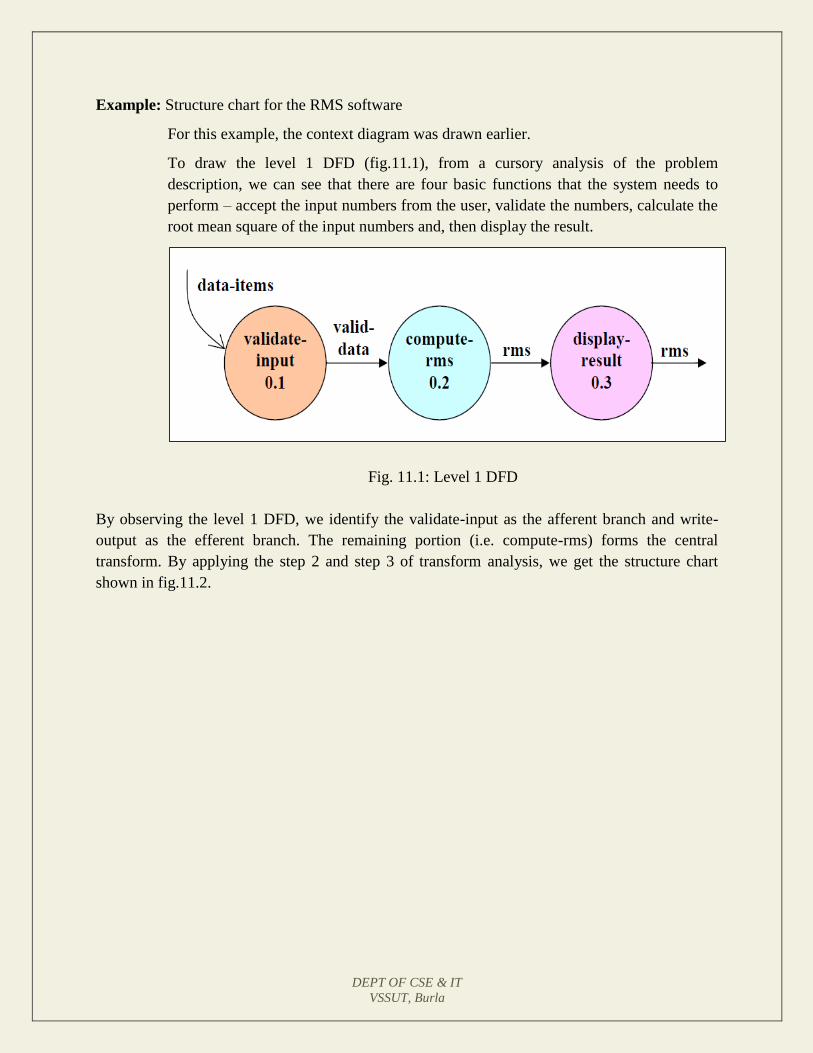
DEPT OF CSE & IT
VSSUT, Burla
Example: Structure chart for the RMS software
For this example, the context diagram was drawn earlier.
To draw the level 1 DFD (fig.11.1), from a cursory analysis of the problem
description, we can see that there are four basic functions that the system needs to
perform – accept the input numbers from the user, validate the numbers, calculate the
root mean square of the input numbers and, then display the result.
Fig. 11.1: Level 1 DFD
By observing the level 1 DFD, we identify the validate-input as the afferent branch and write-
output as the efferent branch. The remaining portion (i.e. compute-rms) forms the central
transform. By applying the step 2 and step 3 of transform analysis, we get the structure chart
shown in fig.11.2.
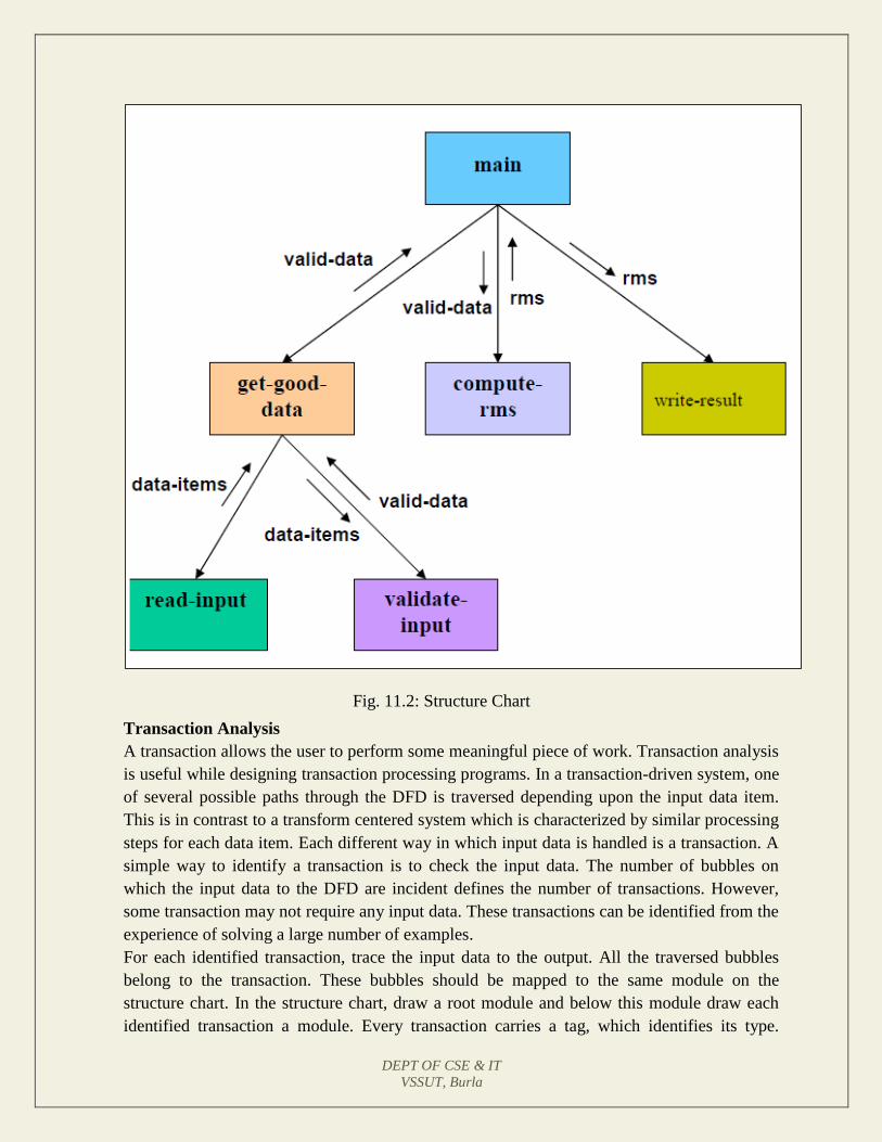
DEPT OF CSE & IT
VSSUT, Burla
Fig. 11.2: Structure Chart
Transaction Analysis
A transaction allows the user to perform some meaningful piece of work. Transaction analysis
is useful while designing transaction processing programs. In a transaction-driven system, one
of several possible paths through the DFD is traversed depending upon the input data item.
This is in contrast to a transform centered system which is characterized by similar processing
steps for each data item. Each different way in which input data is handled is a transaction. A
simple way to identify a transaction is to check the input data. The number of bubbles on
which the input data to the DFD are incident defines the number of transactions. However,
some transaction may not require any input data. These transactions can be identified from the
experience of solving a large number of examples.
For each identified transaction, trace the input data to the output. All the traversed bubbles
belong to the transaction. These bubbles should be mapped to the same module on the
structure chart. In the structure chart, draw a root module and below this module draw each
identified transaction a module. Every transaction carries a tag, which identifies its type.
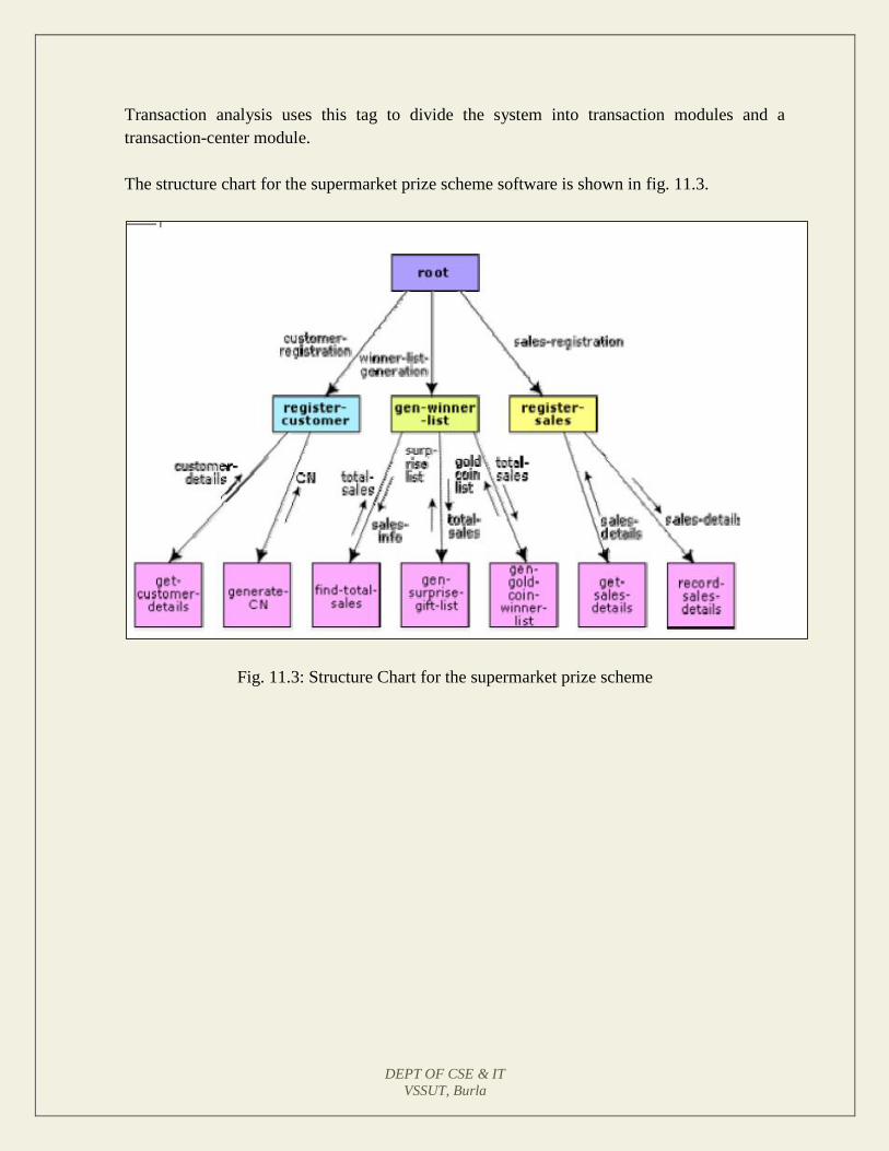
DEPT OF CSE & IT
VSSUT, Burla
Transaction analysis uses this tag to divide the system into transaction modules and a
transaction-center module.
The structure chart for the supermarket prize scheme software is shown in fig. 11.3.
Fig. 11.3: Structure Chart for the supermarket prize scheme
DEPT OF CSE & IT
VSSUT, Burla
MODULE 2
LECTURE NOTE 12
OBJECT MODELLING USING UML
Model
A model captures aspects important for some application while omitting (or abstracting) the rest.
A model in the context of software development can be graphical, textual, mathematical, or
program code-based. Models are very useful in documenting the design and analysis results.
Models also facilitate the analysis and design procedures themselves. Graphical models are very
popular because they are easy to understand and construct. UML is primarily a graphical
modeling tool. However, it often requires text explanations to accompany the graphical models.
Need for a model
An important reason behind constructing a model is that it helps manage complexity. Once
models of a system have been constructed, these can be used for a variety of purposes during
software development, including the following:
• Analysis
• Specification
• Code generation
• Design
• Visualize and understand the problem and the working of a system
• Testing, etc.
In all these applications, the UML models can not only be used to document the results but also
to arrive at the results themselves. Since a model can be used for a variety of purposes, it is
reasonable to expect that the model would vary depending on the purpose for which it is being
constructed. For example, a model developed for initial analysis and specification should be very
different from the one used for design. A model that is being used for analysis and specification
would not show any of the design decisions that would be made later on during the design stage.
On the other hand, a model used for design purposes should capture all the design decisions.
Therefore, it is a good idea to explicitly mention the purpose for which a model has been
developed, along with the model.
DEPT OF CSE & IT
VSSUT, Burla
Unified Modeling Language (UML)
UML, as the name implies, is a modeling language. It may be used to visualize, specify,
construct, and document the artifacts of a software system. It provides a set of notations (e.g.
rectangles, lines, ellipses, etc.) to create a visual model of the system. Like any other language,
UML has its own syntax (symbols and sentence formation rules) and semantics (meanings of
symbols and sentences). Also, we should clearly understand that UML is not a system design or
development methodology, but can be used to document object-oriented and analysis results
obtained using some methodology.
Origin of UML
In the late 1980s and early 1990s, there was a proliferation of object-oriented design techniques
and notations. Different software development houses were using different notations to
document their object-oriented designs. These diverse notations used to give rise to a lot of
confusion.
UML was developed to standardize the large number of object-oriented modeling notations that
existed and were used extensively in the early 1990s. The principles ones in use were:
• Object Management Technology [Rumbaugh 1991]
• Booch’s methodology [Booch 1991]
• Object-Oriented Software Engineering [Jacobson 1992]
• Odell’s methodology [Odell 1992]
• Shaler and Mellor methodology [Shaler 1992]
It is needless to say that UML has borrowed many concepts from these modeling techniques.
Especially, concepts from the first three methodologies have been heavily drawn upon. UML
was adopted by Object Management Group (OMG) as a de facto standard in 1997. OMG is an
association of industries which tries to facilitate early formation of standards.
We shall see that UML contains an extensive set of notations and suggests construction of many
types of diagrams. It has successfully been used to model both large and small problems. The
elegance of UML, its adoption by OMG, and a strong industry backing have helped UML find
widespread acceptance. UML is now being used in a large number of software development
projects worldwide.
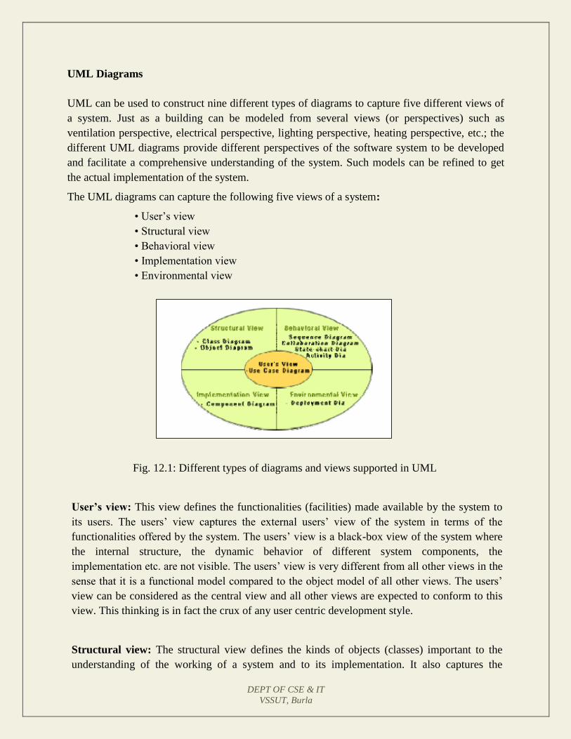
DEPT OF CSE & IT
VSSUT, Burla
UML Diagrams
UML can be used to construct nine different types of diagrams to capture five different views of
a system. Just as a building can be modeled from several views (or perspectives) such as
ventilation perspective, electrical perspective, lighting perspective, heating perspective, etc.; the
different UML diagrams provide different perspectives of the software system to be developed
and facilitate a comprehensive understanding of the system. Such models can be refined to get
the actual implementation of the system.
The UML diagrams can capture the following five views of a system:
• User’s view
• Structural view
• Behavioral view
• Implementation view
• Environmental view
Fig. 12.1: Different types of diagrams and views supported in UML
User’s view: This view defines the functionalities (facilities) made available by the system to
its users. The users’ view captures the external users’ view of the system in terms of the
functionalities offered by the system. The users’ view is a black-box view of the system where
the internal structure, the dynamic behavior of different system components, the
implementation etc. are not visible. The users’ view is very different from all other views in the
sense that it is a functional model compared to the object model of all other views. The users’
view can be considered as the central view and all other views are expected to conform to this
view. This thinking is in fact the crux of any user centric development style.
Structural view: The structural view defines the kinds of objects (classes) important to the
understanding of the working of a system and to its implementation. It also captures the
DEPT OF CSE & IT
VSSUT, Burla
relationships among the classes (objects). The structural model is also called the static model,
since the structure of a system does not change with time.
Behavioral view: The behavioral view captures how objects interact with each other to realize
the system behavior. The system behavior captures the time-dependent (dynamic) behavior of
the system.
Implementation view: This view captures the important components of the system and their
dependencies.
Environmental view: This view models how the different components are implemented on
different pieces of hardware.
DEPT OF CSE & IT
VSSUT, Burla
LECTURE NOTE 13
USE CASE DIAGRAM
Use Case Model
The use case model for any system consists of a set of “use cases”. Intuitively, use cases
represent the different ways in which a system can be used by the users. A simple way to find all
the use cases of a system is to ask the question: “What the users can do using the system?” Thus
for the Library Information System (LIS), the use cases could be:
• issue-book
• query-book
• return-book
• create-member
• add-book, etc
Use cases correspond to the high-level functional requirements. The use cases partition the
system behavior into transactions, such that each transaction performs some useful action from
the user’s point of view. To complete each transaction may involve either a single message or
multiple message exchanges between the user and the system to complete.
Purpose of use cases
The purpose of a use case is to define a piece of coherent behavior without revealing the internal
structure of the system. The use cases do not mention any specific algorithm to be used or the
internal data representation, internal structure of the software, etc. A use case typically
represents a sequence of interactions between the user and the system. These interactions consist
of one mainline sequence. The mainline sequence represents the normal interaction between a
user and the system. The mainline sequence is the most occurring sequence of interaction. For
example, the mainline sequence of the withdraw cash use case supported by a bank ATM drawn,
complete the transaction, and get the amount. Several variations to the main line sequence may
also exist. Typically, a variation from the mainline sequence occurs when some specific
conditions hold. For the bank ATM example, variations or alternate scenarios may occur, if the
password is invalid or the amount to be withdrawn exceeds the amount balance. The variations
are also called alternative paths. A use case can be viewed as a set of related scenarios tied
together by a common goal. The mainline sequence and each of the variations are called
scenarios or instances of the use case. Each scenario is a single path of user events and system
activity through the use case.
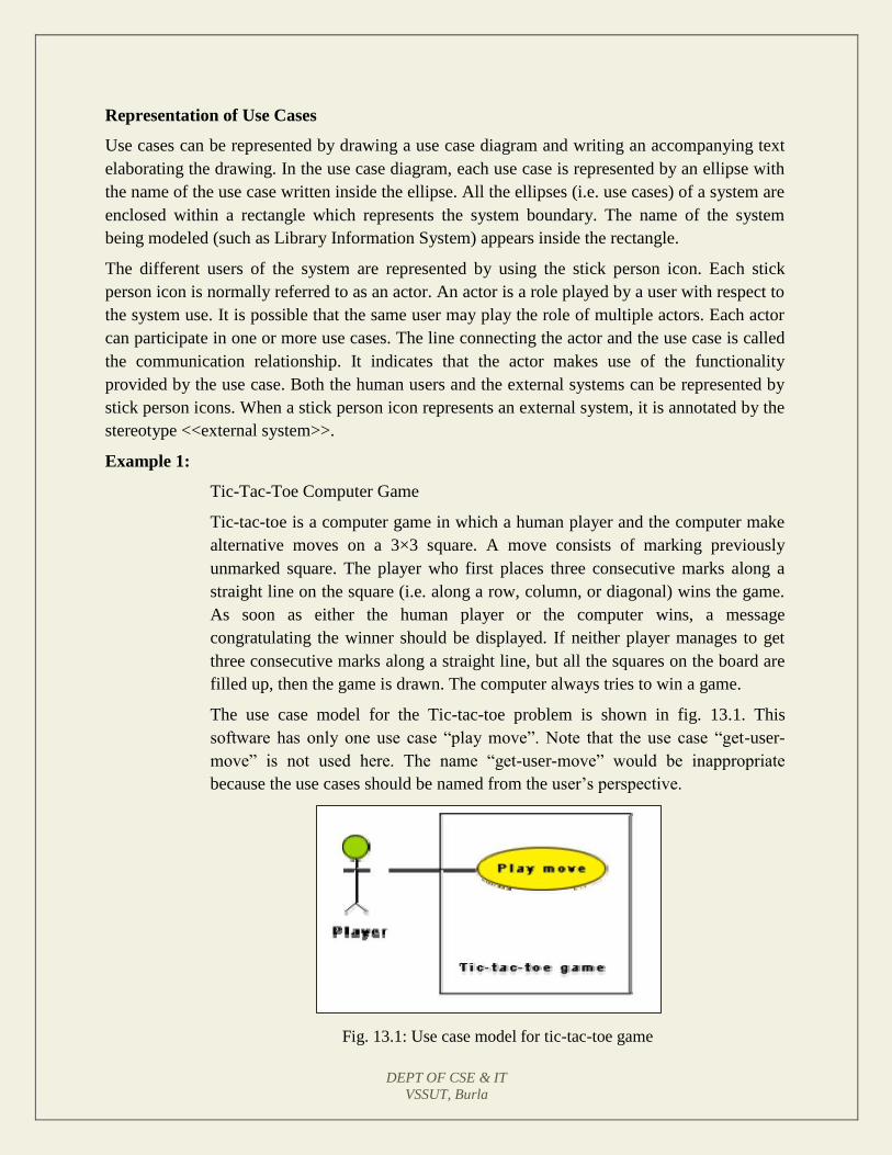
DEPT OF CSE & IT
VSSUT, Burla
Representation of Use Cases
Use cases can be represented by drawing a use case diagram and writing an accompanying text
elaborating the drawing. In the use case diagram, each use case is represented by an ellipse with
the name of the use case written inside the ellipse. All the ellipses (i.e. use cases) of a system are
enclosed within a rectangle which represents the system boundary. The name of the system
being modeled (such as Library Information System) appears inside the rectangle.
The different users of the system are represented by using the stick person icon. Each stick
person icon is normally referred to as an actor. An actor is a role played by a user with respect to
the system use. It is possible that the same user may play the role of multiple actors. Each actor
can participate in one or more use cases. The line connecting the actor and the use case is called
the communication relationship. It indicates that the actor makes use of the functionality
provided by the use case. Both the human users and the external systems can be represented by
stick person icons. When a stick person icon represents an external system, it is annotated by the
stereotype <<external system>>.
Example 1:
Tic-Tac-Toe Computer Game
Tic-tac-toe is a computer game in which a human player and the computer make
alternative moves on a 3×3 square. A move consists of marking previously
unmarked square. The player who first places three consecutive marks along a
straight line on the square (i.e. along a row, column, or diagonal) wins the game.
As soon as either the human player or the computer wins, a message
congratulating the winner should be displayed. If neither player manages to get
three consecutive marks along a straight line, but all the squares on the board are
filled up, then the game is drawn. The computer always tries to win a game.
The use case model for the Tic-tac-toe problem is shown in fig. 13.1. This
software has only one use case “play move”. Note that the use case “get-user-
move” is not used here. The name “get-user-move” would be inappropriate
because the use cases should be named from the user’s perspective.
Fig. 13.1: Use case model for tic-tac-toe game
DEPT OF CSE & IT
VSSUT, Burla
Text Description
Each ellipse on the use case diagram should be accompanied by a text description. The text
description should define the details of the interaction between the user and the computer and
other aspects of the use case. It should include all the behavior associated with the use case in
terms of the mainline sequence, different variations to the normal behavior, the system responses
associated with the use case, the exceptional conditions that may occur in the behavior, etc. The
behavior description is often written in a conversational style describing the interactions between
the actor and the system. The text description may be informal, but some structuring is
recommended. The following are some of the information which may be included in a use case
text description in addition to the mainline sequence, and the alternative scenarios.
Contact persons: This section lists the personnel of the client organization with whom the use
case was discussed, date and time of the meeting, etc.
Actors: In addition to identifying the actors, some information about actors using this use case
which may help the implementation of the use case may be recorded.
Pre-condition: The preconditions would describe the state of the system before the use case
execution starts.
Post-condition: This captures the state of the system after the use case has successfully
completed.
Non-functional requirements: This could contain the important constraints for the design and
implementation, such as platform and environment conditions, qualitative statements, response
time requirements, etc.
Exceptions, error situations: This contains only the domain-related errors such as lack of
user’s access rights, invalid entry in the input fields, etc. Obviously, errors that are not domain
related, such as software errors, need not be discussed here.
Sample dialogs: These serve as examples illustrating the use case.
Specific user interface requirements: These contain specific requirements for the user
interface of the use case. For example, it may contain forms to be used, screen shots, interaction
style, etc.
Document references: This part contains references to specific domain-related documents
which may be useful to understand the system operation
Example 2:
A supermarket needs to develop the following software to encourage regular
customers. For this, the customer needs to supply his/her residence address,
telephone number, and the driving license number. Each customer who registers
for this scheme is assigned a unique customer number (CN) by the computer. A
customer can present his CN to the checkout staff when he makes any purchase.
In this case, the value of his purchase is credited against his CN. At the end of

DEPT OF CSE & IT
VSSUT, Burla
each year, the supermarket intends to award surprise gifts to 10 customers who
make the highest total purchase over the year. Also, it intends to award a 22 caret
gold coin to every customer whose purchase exceeded Rs.10,000. The entries
against the CN are the reset on the day of every year after the prize winners’ lists
are generated.
The use case model for the Supermarket Prize Scheme is shown in fig. 13.2. As discussed
earlier, the use cases correspond to the high-level functional requirements. From the problem
description, we can identify three use cases: “register-customer”, “register-sales”, and “select-
winners”. As a sample, the text description for the use case “register-customer” is shown.
Fig. 13.2 Use case model for Supermarket Prize Scheme
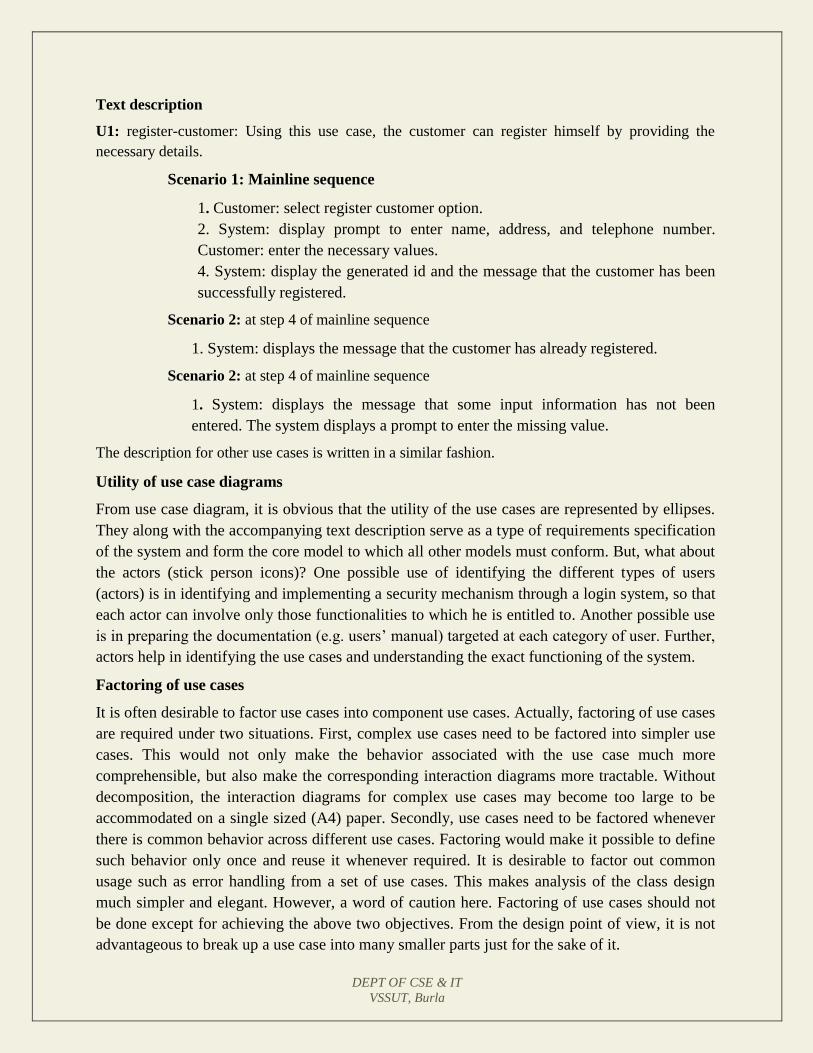
DEPT OF CSE & IT
VSSUT, Burla
Text description
U1: register-customer: Using this use case, the customer can register himself by providing the
necessary details.
Scenario 1: Mainline sequence
1. Customer: select register customer option.
2. System: display prompt to enter name, address, and telephone number.
Customer: enter the necessary values.
4. System: display the generated id and the message that the customer has been
successfully registered.
Scenario 2: at step 4 of mainline sequence
1. System: displays the message that the customer has already registered.
Scenario 2: at step 4 of mainline sequence
1. System: displays the message that some input information has not been
entered. The system displays a prompt to enter the missing value.
The description for other use cases is written in a similar fashion.
Utility of use case diagrams
From use case diagram, it is obvious that the utility of the use cases are represented by ellipses.
They along with the accompanying text description serve as a type of requirements specification
of the system and form the core model to which all other models must conform. But, what about
the actors (stick person icons)? One possible use of identifying the different types of users
(actors) is in identifying and implementing a security mechanism through a login system, so that
each actor can involve only those functionalities to which he is entitled to. Another possible use
is in preparing the documentation (e.g. users’ manual) targeted at each category of user. Further,
actors help in identifying the use cases and understanding the exact functioning of the system.
Factoring of use cases
It is often desirable to factor use cases into component use cases. Actually, factoring of use cases
are required under two situations. First, complex use cases need to be factored into simpler use
cases. This would not only make the behavior associated with the use case much more
comprehensible, but also make the corresponding interaction diagrams more tractable. Without
decomposition, the interaction diagrams for complex use cases may become too large to be
accommodated on a single sized (A4) paper. Secondly, use cases need to be factored whenever
there is common behavior across different use cases. Factoring would make it possible to define
such behavior only once and reuse it whenever required. It is desirable to factor out common
usage such as error handling from a set of use cases. This makes analysis of the class design
much simpler and elegant. However, a word of caution here. Factoring of use cases should not
be done except for achieving the above two objectives. From the design point of view, it is not
advantageous to break up a use case into many smaller parts just for the sake of it.
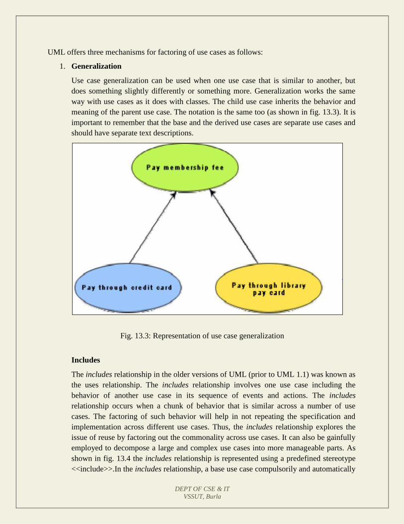
DEPT OF CSE & IT
VSSUT, Burla
UML offers three mechanisms for factoring of use cases as follows:
1. Generalization
Use case generalization can be used when one use case that is similar to another, but
does something slightly differently or something more. Generalization works the same
way with use cases as it does with classes. The child use case inherits the behavior and
meaning of the parent use case. The notation is the same too (as shown in fig. 13.3). It is
important to remember that the base and the derived use cases are separate use cases and
should have separate text descriptions.
Fig. 13.3: Representation of use case generalization
Includes
The includes relationship in the older versions of UML (prior to UML 1.1) was known as
the uses relationship. The includes relationship involves one use case including the
behavior of another use case in its sequence of events and actions. The includes
relationship occurs when a chunk of behavior that is similar across a number of use
cases. The factoring of such behavior will help in not repeating the specification and
implementation across different use cases. Thus, the includes relationship explores the
issue of reuse by factoring out the commonality across use cases. It can also be gainfully
employed to decompose a large and complex use cases into more manageable parts. As
shown in fig. 13.4 the includes relationship is represented using a predefined stereotype
<<include>>.In the includes relationship, a base use case compulsorily and automatically

DEPT OF CSE & IT
VSSUT, Burla
includes the behavior of the common use cases. As shown in example fig. 13.5, issue-
book and renew-book both include check-reservation use case. The base use case may
include several use cases. In such cases, it may interleave their associated common use
cases together. The common use case becomes a separate use case and the independent
text description should be provided for it.
Fig. 13.4 Representation of use case inclusion
Fig. 13.5: Example use case inclusion
Extends
The main idea behind the extends relationship among the use cases is that it allows you to
show optional system behavior. An optional system behavior is extended only under certain
conditions. This relationship among use cases is also predefined as a stereotype as shown in
fig. 13.6. The extends relationship is similar to generalization. But unlike generalization, the
extending use case can add additional behavior only at an extension point only when certain
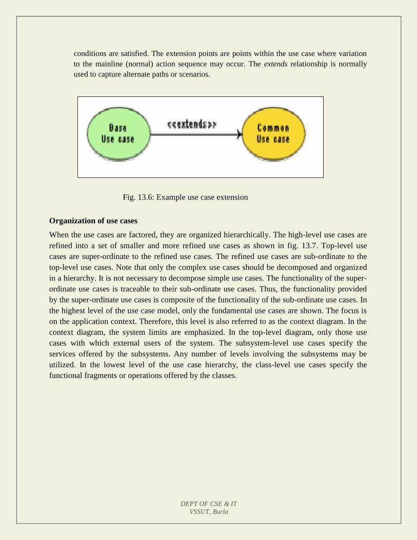
DEPT OF CSE & IT
VSSUT, Burla
conditions are satisfied. The extension points are points within the use case where variation
to the mainline (normal) action sequence may occur. The extends relationship is normally
used to capture alternate paths or scenarios.
Fig. 13.6: Example use case extension
Organization of use cases
When the use cases are factored, they are organized hierarchically. The high-level use cases are
refined into a set of smaller and more refined use cases as shown in fig. 13.7. Top-level use
cases are super-ordinate to the refined use cases. The refined use cases are sub-ordinate to the
top-level use cases. Note that only the complex use cases should be decomposed and organized
in a hierarchy. It is not necessary to decompose simple use cases. The functionality of the super-
ordinate use cases is traceable to their sub-ordinate use cases. Thus, the functionality provided
by the super-ordinate use cases is composite of the functionality of the sub-ordinate use cases. In
the highest level of the use case model, only the fundamental use cases are shown. The focus is
on the application context. Therefore, this level is also referred to as the context diagram. In the
context diagram, the system limits are emphasized. In the top-level diagram, only those use
cases with which external users of the system. The subsystem-level use cases specify the
services offered by the subsystems. Any number of levels involving the subsystems may be
utilized. In the lowest level of the use case hierarchy, the class-level use cases specify the
functional fragments or operations offered by the classes.
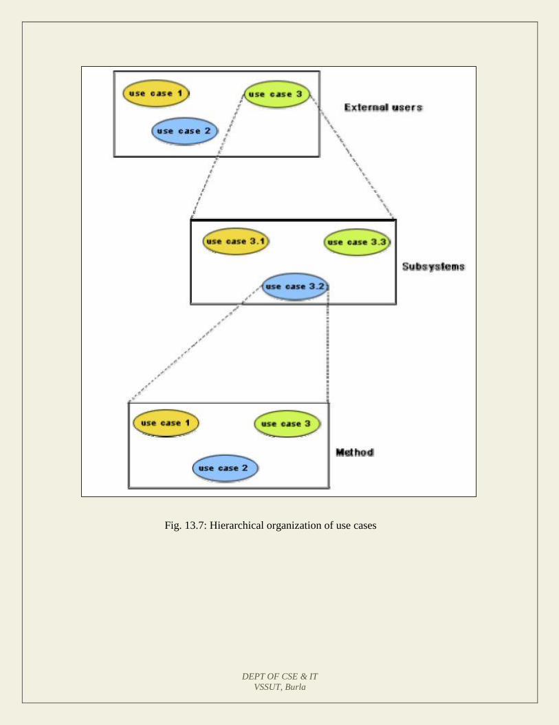
DEPT OF CSE & IT
VSSUT, Burla
Fig. 13.7: Hierarchical organization of use cases

DEPT OF CSE & IT
VSSUT, Burla
LECTURE NOTE 14
CLASS DIAGRAMS
A class diagram describes the static structure of a system. It shows how a system is structured rather
than how it behaves. The static structure of a system comprises of a number of class diagrams and
their dependencies. The main constituents of a class diagram are classes and their relationships:
generalization, aggregation, association, and various kinds of dependencies.
Classes
The classes represent entities with common features, i.e. attributes and operations. Classes are
represented as solid outline rectangles with compartments. Classes have a mandatory name
compartment where the name is written centered in boldface. The class name is usually written using
mixed case convention and begins with an uppercase. The class names are usually chosen to be
singular nouns. Classes have optional attributes and operations compartments. A class may appear on
several diagrams. Its attributes and operations are suppressed on all but one diagram.
Attributes
An attribute is a named property of a class. It represents the kind of data that an object might contain.
Attributes are listed with their names, and may optionally contain specification of their type, an
initial value, and constraints. The type of the attribute is written by appending a colon and the type
name after the attribute name. Typically, the first letter of a class name is a small letter. An example
for an attribute is given.
bookName : String
Operation
Operation is the implementation of a service that can be requested from any object of the class to
affect behaviour. An object’s data or state can be changed by invoking an operation of the object. A
class may have any number of operations or no operation at all. Typically, the first letter of an
operation name is a small letter. Abstract operations are written in italics. The parameters of an
operation (if any), may have a kind specified, which may be ‘in’, ‘out’ or ‘inout’. An operation may
have a return type consisting of a single return type expression. An example for an operation is given.
issueBook(in bookName):Boolean
Association
Associations are needed to enable objects to communicate with each other. An association describes
a connection between classes. The association relation between two objects is called object
connection or link. Links are instances of associations. A link is a physical or conceptual connection
between object instances. For example, suppose Amit has borrowed the book Graph Theory. Here,
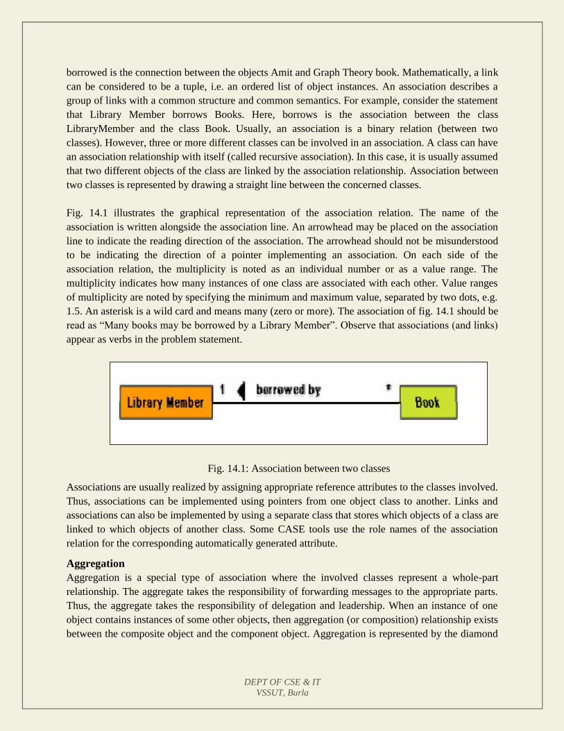
DEPT OF CSE & IT
VSSUT, Burla
borrowed is the connection between the objects Amit and Graph Theory book. Mathematically, a link
can be considered to be a tuple, i.e. an ordered list of object instances. An association describes a
group of links with a common structure and common semantics. For example, consider the statement
that Library Member borrows Books. Here, borrows is the association between the class
LibraryMember and the class Book. Usually, an association is a binary relation (between two
classes). However, three or more different classes can be involved in an association. A class can have
an association relationship with itself (called recursive association). In this case, it is usually assumed
that two different objects of the class are linked by the association relationship. Association between
two classes is represented by drawing a straight line between the concerned classes.
Fig. 14.1 illustrates the graphical representation of the association relation. The name of the
association is written alongside the association line. An arrowhead may be placed on the association
line to indicate the reading direction of the association. The arrowhead should not be misunderstood
to be indicating the direction of a pointer implementing an association. On each side of the
association relation, the multiplicity is noted as an individual number or as a value range. The
multiplicity indicates how many instances of one class are associated with each other. Value ranges
of multiplicity are noted by specifying the minimum and maximum value, separated by two dots, e.g.
1.5. An asterisk is a wild card and means many (zero or more). The association of fig. 14.1 should be
read as “Many books may be borrowed by a Library Member”. Observe that associations (and links)
appear as verbs in the problem statement.
Fig. 14.1: Association between two classes
Associations are usually realized by assigning appropriate reference attributes to the classes involved.
Thus, associations can be implemented using pointers from one object class to another. Links and
associations can also be implemented by using a separate class that stores which objects of a class are
linked to which objects of another class. Some CASE tools use the role names of the association
relation for the corresponding automatically generated attribute.
Aggregation
Aggregation is a special type of association where the involved classes represent a whole-part
relationship. The aggregate takes the responsibility of forwarding messages to the appropriate parts.
Thus, the aggregate takes the responsibility of delegation and leadership. When an instance of one
object contains instances of some other objects, then aggregation (or composition) relationship exists
between the composite object and the component object. Aggregation is represented by the diamond
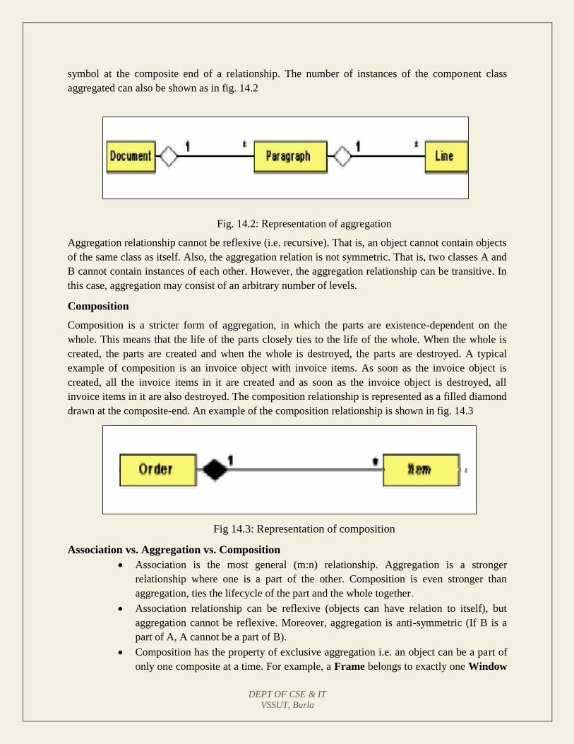
DEPT OF CSE & IT
VSSUT, Burla
symbol at the composite end of a relationship. The number of instances of the component class
aggregated can also be shown as in fig. 14.2
Fig. 14.2: Representation of aggregation
Aggregation relationship cannot be reflexive (i.e. recursive). That is, an object cannot contain objects
of the same class as itself. Also, the aggregation relation is not symmetric. That is, two classes A and
B cannot contain instances of each other. However, the aggregation relationship can be transitive. In
this case, aggregation may consist of an arbitrary number of levels.
Composition
Composition is a stricter form of aggregation, in which the parts are existence-dependent on the
whole. This means that the life of the parts closely ties to the life of the whole. When the whole is
created, the parts are created and when the whole is destroyed, the parts are destroyed. A typical
example of composition is an invoice object with invoice items. As soon as the invoice object is
created, all the invoice items in it are created and as soon as the invoice object is destroyed, all
invoice items in it are also destroyed. The composition relationship is represented as a filled diamond
drawn at the composite-end. An example of the composition relationship is shown in fig. 14.3
Fig 14.3: Representation of composition
Association vs. Aggregation vs. Composition
Association is the most general (m:n) relationship. Aggregation is a stronger
relationship where one is a part of the other. Composition is even stronger than
aggregation, ties the lifecycle of the part and the whole together.
Association relationship can be reflexive (objects can have relation to itself), but
aggregation cannot be reflexive. Moreover, aggregation is anti-symmetric (If B is a
part of A, A cannot be a part of B).
Composition has the property of exclusive aggregation i.e. an object can be a part of
only one composite at a time. For example, a Frame belongs to exactly one Window
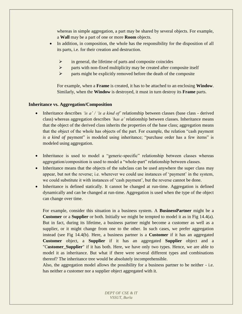
DEPT OF CSE & IT
VSSUT, Burla
whereas in simple aggregation, a part may be shared by several objects. For example,
a Wall may be a part of one or more Room objects.
In addition, in composition, the whole has the responsibility for the disposition of all
its parts, i.e. for their creation and destruction.
in general, the lifetime of parts and composite coincides
parts with non-fixed multiplicity may be created after composite itself
parts might be explicitly removed before the death of the composite
For example, when a Frame is created, it has to be attached to an enclosing Window.
Similarly, when the Window is destroyed, it must in turn destroy its Frame parts.
Inheritance vs. Aggregation/Composition
Inheritance describes ‘is a’ / ‘is a kind of’ relationship between classes (base class - derived
class) whereas aggregation describes ‘has a’ relationship between classes. Inheritance means
that the object of the derived class inherits the properties of the base class; aggregation means
that the object of the whole has objects of the part. For example, the relation “cash payment
is a kind of payment” is modeled using inheritance; “purchase order has a few items” is
modeled using aggregation.
Inheritance is used to model a “generic-specific” relationship between classes whereas
aggregation/composition is used to model a “whole-part” relationship between classes.
Inheritance means that the objects of the subclass can be used anywhere the super class may
appear, but not the reverse; i.e. wherever we could use instances of ‘payment’ in the system,
we could substitute it with instances of ‘cash payment’, but the reverse cannot be done.
Inheritance is defined statically. It cannot be changed at run-time. Aggregation is defined
dynamically and can be changed at run-time. Aggregation is used when the type of the object
can change over time.
For example, consider this situation in a business system. A BusinessPartner might be a
Customer or a Supplier or both. Initially we might be tempted to model it as in Fig 14.4(a).
But in fact, during its lifetime, a business partner might become a customer as well as a
supplier, or it might change from one to the other. In such cases, we prefer aggregation
instead (see Fig 14.4(b). Here, a business partner is a Customer if it has an aggregated
Customer object, a Supplier if it has an aggregated Supplier object and a
"Customer_Supplier" if it has both. Here, we have only two types. Hence, we are able to
model it as inheritance. But what if there were several different types and combinations
thereof? The inheritance tree would be absolutely incomprehensible.
Also, the aggregation model allows the possibility for a business partner to be neither - i.e.
has neither a customer nor a supplier object aggregated with it.
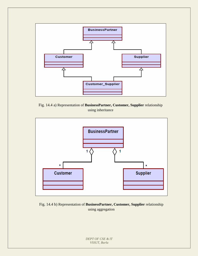
DEPT OF CSE & IT
VSSUT, Burla
Fig. 14.4 a) Representation of BusinessPartner, Customer, Supplier relationship
using inheritance
Fig. 14.4 b) Representation of BusinessPartner, Customer, Supplier relationship
using aggregation

DEPT OF CSE & IT
VSSUT, Burla
• The advantage of aggregation is the integrity of encapsulation. The operations of an object are the
interfaces of other objects which imply low implementation dependencies. The significant
disadvantage of aggregation is the increase in the number of objects and their relationships. On the
other hand, inheritance allows for an easy way to modify implementation for reusability. But the
significant disadvantage is that it breaks encapsulation, which implies implementation dependence.
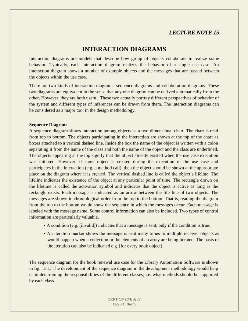
DEPT OF CSE & IT
VSSUT, Burla
LECTURE NOTE 15
INTERACTION DIAGRAMS
Interaction diagrams are models that describe how group of objects collaborate to realize some
behavior. Typically, each interaction diagram realizes the behavior of a single use case. An
interaction diagram shows a number of example objects and the messages that are passed between
the objects within the use case.
There are two kinds of interaction diagrams: sequence diagrams and collaboration diagrams. These
two diagrams are equivalent in the sense that any one diagram can be derived automatically from the
other. However, they are both useful. These two actually portray different perspectives of behavior of
the system and different types of inferences can be drawn from them. The interaction diagrams can
be considered as a major tool in the design methodology.
Sequence Diagram
A sequence diagram shows interaction among objects as a two dimensional chart. The chart is read
from top to bottom. The objects participating in the interaction are shown at the top of the chart as
boxes attached to a vertical dashed line. Inside the box the name of the object is written with a colon
separating it from the name of the class and both the name of the object and the class are underlined.
The objects appearing at the top signify that the object already existed when the use case execution
was initiated. However, if some object is created during the execution of the use case and
participates in the interaction (e.g. a method call), then the object should be shown at the appropriate
place on the diagram where it is created. The vertical dashed line is called the object’s lifeline. The
lifeline indicates the existence of the object at any particular point of time. The rectangle drawn on
the lifetime is called the activation symbol and indicates that the object is active as long as the
rectangle exists. Each message is indicated as an arrow between the life line of two objects. The
messages are shown in chronological order from the top to the bottom. That is, reading the diagram
from the top to the bottom would show the sequence in which the messages occur. Each message is
labeled with the message name. Some control information can also be included. Two types of control
information are particularly valuable.
• A condition (e.g. [invalid]) indicates that a message is sent, only if the condition is true.
• An iteration marker shows the message is sent many times to multiple receiver objects as
would happen when a collection or the elements of an array are being iterated. The basis of
the iteration can also be indicated e.g. [for every book object].
The sequence diagram for the book renewal use case for the Library Automation Software is shown
in fig. 15.1. The development of the sequence diagram in the development methodology would help
us in determining the responsibilities of the different classes; i.e. what methods should be supported
by each class.
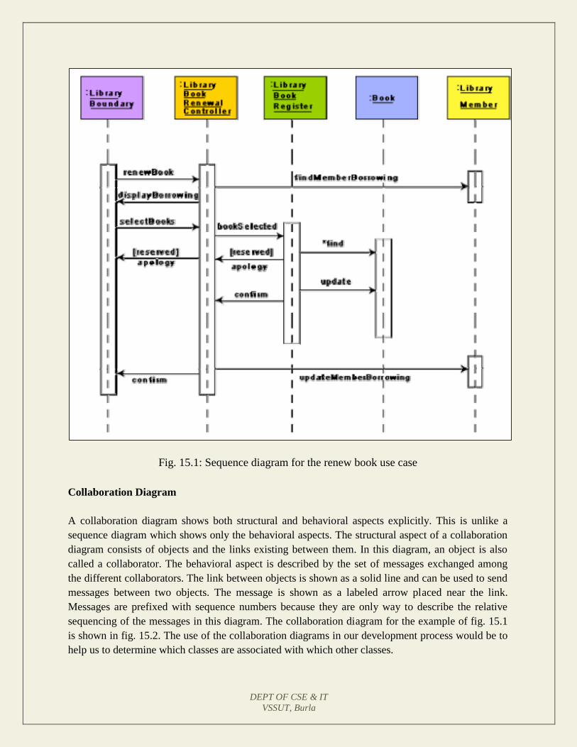
DEPT OF CSE & IT
VSSUT, Burla
Fig. 15.1: Sequence diagram for the renew book use case
Collaboration Diagram
A collaboration diagram shows both structural and behavioral aspects explicitly. This is unlike a
sequence diagram which shows only the behavioral aspects. The structural aspect of a collaboration
diagram consists of objects and the links existing between them. In this diagram, an object is also
called a collaborator. The behavioral aspect is described by the set of messages exchanged among
the different collaborators. The link between objects is shown as a solid line and can be used to send
messages between two objects. The message is shown as a labeled arrow placed near the link.
Messages are prefixed with sequence numbers because they are only way to describe the relative
sequencing of the messages in this diagram. The collaboration diagram for the example of fig. 15.1
is shown in fig. 15.2. The use of the collaboration diagrams in our development process would be to
help us to determine which classes are associated with which other classes.
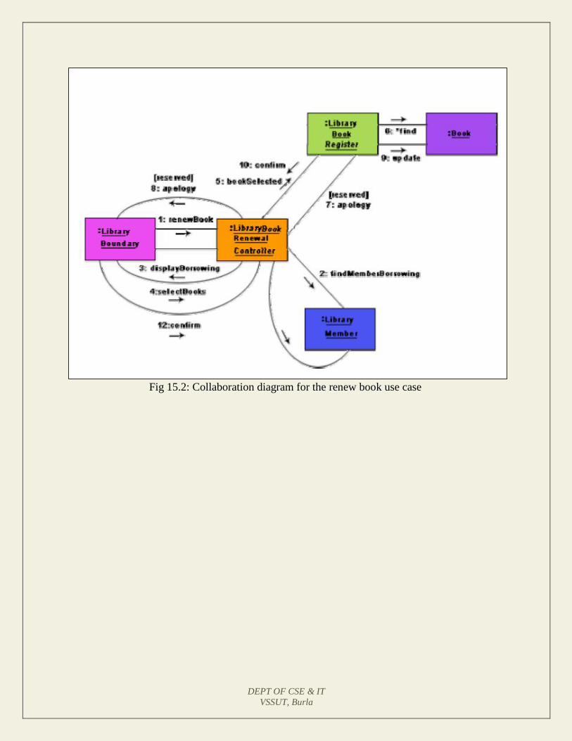
DEPT OF CSE & IT
VSSUT, Burla
Fig 15.2: Collaboration diagram for the renew book use case
DEPT OF CSE & IT
VSSUT, Burla
LECTURE NOTE 16
ACTIVITY AND STATE CHART DIAGRAM
The activity diagram is possibly one modeling element which was not present in any of the
predecessors of UML. No such diagrams were present either in the works of Booch, Jacobson, or
Rumbaugh. It is possibly based on the event diagram of Odell [1992] through the notation is very
different from that used by Odell. The activity diagram focuses on representing activities or chunks
of processing which may or may not correspond to the methods of classes. An activity is a state with
an internal action and one or more outgoing transitions which automatically follow the termination
of the internal activity. If an activity has more than one outgoing transitions, then these must be
identified through conditions. An interesting feature of the activity diagrams is the swim lanes. Swim
lanes enable you to group activities based on who is performing them, e.g. academic department vs.
hostel office. Thus swim lanes subdivide activities based on the responsibilities of some components.
The activities in a swim lane can be assigned to some model elements, e.g. classes or some
component, etc.
Activity diagrams are normally employed in business process modeling. This is carried out during
the initial stages of requirements analysis and specification. Activity diagrams can be very useful to
understand complex processing activities involving many components. Later these diagrams can be
used to develop interaction diagrams which help to allocate activities (responsibilities) to classes.
The student admission process in a university is shown as an activity diagram in fig. 16.1. This
shows the part played by different components of the Institute in the admission procedure. After the
fees are received at the account section, parallel activities start at the hostel office, hospital, and the
Department. After all these activities complete (this synchronization is represented as a horizontal
line), the identity card can be issued to a student by the Academic section.
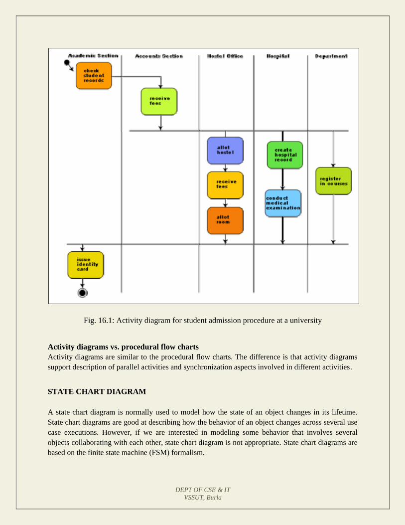
DEPT OF CSE & IT
VSSUT, Burla
Fig. 16.1: Activity diagram for student admission procedure at a university
Activity diagrams vs. procedural flow charts
Activity diagrams are similar to the procedural flow charts. The difference is that activity diagrams
support description of parallel activities and synchronization aspects involved in different activities.
STATE CHART DIAGRAM
A state chart diagram is normally used to model how the state of an object changes in its lifetime.
State chart diagrams are good at describing how the behavior of an object changes across several use
case executions. However, if we are interested in modeling some behavior that involves several
objects collaborating with each other, state chart diagram is not appropriate. State chart diagrams are
based on the finite state machine (FSM) formalism.
DEPT OF CSE & IT
VSSUT, Burla
A FSM consists of a finite number of states corresponding to those of the object being modeled. The
object undergoes state changes when specific events occur. The FSM formalism existed long before
the object-oriented technology and has been used for a wide variety of applications. Apart from
modeling, it has even been used in theoretical computer science as a generator for regular languages.
A major disadvantage of the FSM formalism is the state explosion problem. The number of states
becomes too many and the model too complex when used to model practical systems. This problem
is overcome in UML by using state charts. The state chart formalism was proposed by David Harel
[1990]. A state chart is a hierarchical model of a system and introduces the concept of a composite
state (also called nested state).
Actions are associated with transitions and are considered to be processes that occur quickly and are
not interruptible. Activities are associated with states and can take longer. An activity can be
interrupted by an event.
The basic elements of the state chart diagram are as follows:
Initial state- This is represented as a filled circle.
Final state- This is represented by a filled circle inside a larger circle.
State- These are represented by rectangles with rounded corners.
Transition- A transition is shown as an arrow between two states. Normally, the name of the
event which causes the transition is places alongside the arrow. A guard to the transition can
also be assigned. A guard is a Boolean logic condition. The transition can take place only if
the grade evaluates to true. The syntax for the label of the transition is shown in 3 parts: event
[guard]/action.
An example state chart for the order object of the Trade House Automation software is shown in fig.
16.2.
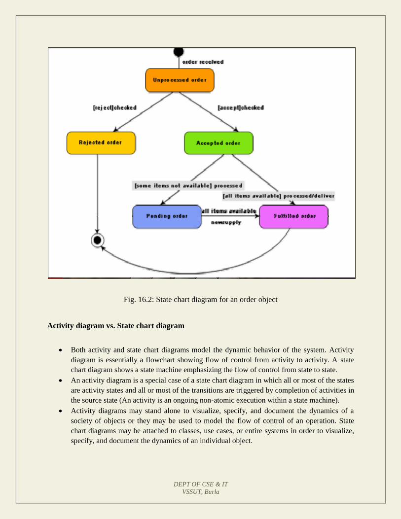
DEPT OF CSE & IT
VSSUT, Burla
Fig. 16.2: State chart diagram for an order object
Activity diagram vs. State chart diagram
Both activity and state chart diagrams model the dynamic behavior of the system. Activity
diagram is essentially a flowchart showing flow of control from activity to activity. A state
chart diagram shows a state machine emphasizing the flow of control from state to state.
An activity diagram is a special case of a state chart diagram in which all or most of the states
are activity states and all or most of the transitions are triggered by completion of activities in
the source state (An activity is an ongoing non-atomic execution within a state machine).
Activity diagrams may stand alone to visualize, specify, and document the dynamics of a
society of objects or they may be used to model the flow of control of an operation. State
chart diagrams may be attached to classes, use cases, or entire systems in order to visualize,
specify, and document the dynamics of an individual object.

DEPT OF CSE & IT
VSSUT, Burla
MODULE 3
LECTURE NOTE 17
CODING
Coding- The objective of the coding phase is to transform the design of a system into code in a
high level language and then to unit test this code. The programmers adhere to standard and well
defined style of coding which they call their coding standard. The main advantages of adhering
to a standard style of coding are as follows:
A coding standard gives uniform appearances to the code written by different
engineers
It facilitates code of understanding.
Promotes good programming practices.
For implementing our design into a code, we require a good high level language. A programming
language should have the following features:
Characteristics of a Programming Language
Readability: A good high-level language will allow programs to be written in some ways
that resemble a quite-English description of the underlying algorithms. If care is taken,
the coding may be done in a way that is essentially self-documenting.
Portability: High-level languages, being essentially machine independent, should be able
to develop portable software.
Generality: Most high-level languages allow the writing of a wide variety of programs,
thus relieving the programmer of the need to become expert in many diverse languages.
Brevity: Language should have the ability to implement the algorithm with less amount
of code. Programs expressed in high-level languages are often considerably shorter than
their low-level equivalents.
Error checking: Being human, a programmer is likely to make many mistakes in the
development of a computer program. Many high-level languages enforce a great deal of
error checking both at compile-time and at run-time.
Cost: The ultimate cost of a programming language is a function of many of its
characteristics.
DEPT OF CSE & IT
VSSUT, Burla
Familiar notation: A language should have familiar notation, so it can be understood by
most of the programmers.
Quick translation: It should admit quick translation.
Efficiency: It should permit the generation of efficient object code.
Modularity: It is desirable that programs can be developed in the language as a
collection of separately compiled modules, with appropriate mechanisms for ensuring
self-consistency between these modules.
Widely available: Language should be widely available and it should be possible to
provide translators for all the major machines and for all the major operating systems.
A coding standard lists several rules to be followed during coding, such as the way variables are
to be named, the way the code is to be laid out, error return conventions, etc.
Coding standards and guidelines
Good software development organizations usually develop their own coding standards and
guidelines depending on what best suits their organization and the type of products they develop.
The following are some representative coding standards.
1. Rules for limiting the use of global: These rules list what types of data can be declared
global and what cannot.
2. Contents of the headers preceding codes for different modules: The information
contained in the headers of different modules should be standard for an organization. The
exact format in which the header information is organized in the header can also be
specified. The following are some standard header data:
• Name of the module.
• Date on which the module was created.
• Author’s name.
• Modification history.
• Synopsis of the module.
• Different functions supported, along with their input/output parameters.
• Global variables accessed/modified by the module.
DEPT OF CSE & IT
VSSUT, Burla
3. Naming conventions for global variables, local variables, and constant identifiers: A
possible naming convention can be that global variable names always start with a capital
letter, local variable names are made of small letters, and constant names are always
capital letters.
4. Error return conventions and exception handling mechanisms: The way error
conditions are reported by different functions in a program are handled should be
standard within an organization. For example, different functions while encountering an
error condition should either return a 0 or 1 consistently.
The following are some representative coding guidelines recommended by many software
development organizations.
1. Do not use a coding style that is too clever or too difficult to understand: Code
should be easy to understand. Many inexperienced engineers actually take pride in
writing cryptic and incomprehensible code. Clever coding can obscure meaning of the
code and hamper understanding. It also makes maintenance difficult.
2. Avoid obscure side effects: The side effects of a function call include modification of
parameters passed by reference, modification of global variables, and I/O operations. An
obscure side effect is one that is not obvious from a casual examination of the code.
Obscure side effects make it difficult to understand a piece of code. For example, if a
global variable is changed obscurely in a called module or some file I/O is performed
which is difficult to infer from the function’s name and header information, it becomes
difficult for anybody trying to understand the code.
3. Do not use an identifier for multiple purposes: Programmers often use the same
identifier to denote several temporary entities. For example, some programmers use a
temporary loop variable for computing and a storing the final result. The rationale that is
usually given by these programmers for such multiple uses of variables is memory
efficiency, e.g. three variables use up three memory locations, whereas the same variable
used in three different ways uses just one memory location. However, there are several
things wrong with this approach and hence should be avoided. Some of the problems
caused by use of variables for multiple purposes as follows:
Each variable should be given a descriptive name indicating its purpose. This is
not possible if an identifier is used for multiple purposes. Use of a variable for
multiple purposes can lead to confusion and make it difficult for somebody trying to
read and understand the code.
DEPT OF CSE & IT
VSSUT, Burla
Use of variables for multiple purposes usually makes future enhancements more
difficult.
4. The code should be well-documented: As a rule of thumb, there must be at least one
comment line on the average for every three-source line.
5. The length of any function should not exceed 10 source lines: A function that is very
lengthy is usually very difficult to understand as it probably carries out many different
functions. For the same reason, lengthy functions are likely to have disproportionately
larger number of bugs.
6. Do not use goto statements: Use of goto statements makes a program unstructured and
very difficult to understand.
Code Review
Code review for a model is carried out after the module is successfully compiled and the all the
syntax errors have been eliminated. Code reviews are extremely cost-effective strategies for
reduction in coding errors and to produce high quality code. Normally, two types of reviews are
carried out on the code of a module. These two types code review techniques are code inspection
and code walk through.
Code Walk Throughs
Code walk through is an informal code analysis technique. In this technique, after a module has
been coded, successfully compiled and all syntax errors eliminated. A few members of the
development team are given the code few days before the walk through meeting to read and
understand code. Each member selects some test cases and simulates execution of the code by
hand (i.e. trace execution through each statement and function execution). The main objectives
of the walk through are to discover the algorithmic and logical errors in the code. The members
note down their findings to discuss these in a walk through meeting where the coder of the
module is present. Even though a code walk through is an informal analysis technique, several
guidelines have evolved over the years for making this naïve but useful analysis technique more
effective. Of course, these guidelines are based on personal experience, common sense, and
several subjective factors. Therefore, these guidelines should be considered as examples rather
than accepted as rules to be applied dogmatically. Some of these guidelines are the following:
The team performing code walk through should not be either too big or too small. Ideally,
it should consist of between three to seven members.
Discussion should focus on discovery of errors and not on how to fix the discovered
errors.

DEPT OF CSE & IT
VSSUT, Burla
In order to foster cooperation and to avoid the feeling among engineers that they are
being evaluated in the code walk through meeting, managers should not attend the walk
through meetings.
Code Inspection
In contrast to code walk through, the aim of code inspection is to discover some common types
of errors caused due to oversight and improper programming. In other words, during code
inspection the code is examined for the presence of certain kinds of errors, in contrast to the hand
simulation of code execution done in code walk throughs. For instance, consider the classical
error of writing a procedure that modifies a formal parameter while the calling routine calls that
procedure with a constant actual parameter. It is more likely that such an error will be discovered
by looking for these kinds of mistakes in the code, rather than by simply hand simulating
execution of the procedure. In addition to the commonly made errors, adherence to coding
standards is also checked during code inspection. Good software development companies collect
statistics regarding different types of errors commonly committed by their engineers and identify
the type of errors most frequently committed. Such a list of commonly committed errors can be
used during code inspection to look out for possible errors.
Following is a list of some classical programming errors which can be checked during code
inspection:
Use of uninitialized variables.
Jumps into loops.
Nonterminating loops.
Incompatible assignments.
Array indices out of bounds.
Improper storage allocation and deallocation.
Mismatches between actual and formal parameter in procedure calls.
Use of incorrect logical operators or incorrect precedence among operators.
Improper modification of loop variables.
Comparison of equally of floating point variables, etc.
Clean Room Testing
Clean room testing was pioneered by IBM. This type of testing relies heavily on walk throughs,
inspection, and formal verification. The programmers are not allowed to test any of their code by
executing the code other than doing some syntax testing using a compiler. The software
development philosophy is based on avoiding software defects by using a rigorous inspection
process. The objective of this software is zero-defect software. The name ‘clean room’ was
derived from the analogy with semi-conductor fabrication units. In these units (clean rooms),
defects are avoided by manufacturing in ultra-clean atmosphere. In this kind of development,
inspections to check the consistency of the components with their specifications has replaced
unit-testing.
DEPT OF CSE & IT
VSSUT, Burla
This technique reportedly produces documentation and code that is more reliable and
maintainable than other development methods relying heavily on code execution-based testing.
The clean room approach to software development is based on five characteristics:
Formal specification: The software to be developed is formally specified. A state-
transition model which shows system responses to stimuli is used to express the
specification.
Incremental development: The software is partitioned into increments which are
developed and validated separately using the clean room process. These increments are
specified, with customer input, at an early stage in the process.
Structured programming: Only a limited number of control and data abstraction
constructs are used. The program development process is process of stepwise refinement
of the specification.
Static verification: The developed software is statically verified using rigorous software
inspections. There is no unit or module testing process for code components
Statistical testing of the system: The integrated software increment is tested statistically
to determine its reliability. These statistical tests are based on the operational profile
which is developed in parallel with the system specification. The main problem with this
approach is that testing effort is increased as walk throughs, inspection, and verification
are time-consuming.
Software Documentation
When various kinds of software products are developed then not only the executable files and the
source code are developed but also various kinds of documents such as users’ manual, software
requirements specification (SRS) documents, design documents, test documents, installation
manual, etc are also developed as part of any software engineering process. All these documents
are a vital part of good software development practice. Good documents are very useful and
server the following purposes:
o Good documents enhance understandability and maintainability of a software
product. They reduce the effort and time required for maintenance.
o Use documents help the users in effectively using the system.
o Good documents help in effectively handling the manpower turnover problem.
Even when an engineer leaves the organization, and a new engineer comes in, he
can build up the required knowledge easily.
o Production of good documents helps the manager in effectively tracking the
progress of the project. The project manager knows that measurable progress is
achieved if a piece of work is done and the required documents have been
produced and reviewed.
DEPT OF CSE & IT
VSSUT, Burla
Different types of software documents can broadly be classified into the following:
• Internal documentation
• External documentation
Internal documentation is the code comprehension features provided as part of the source code
itself. Internal documentation is provided through appropriate module headers and comments
embedded in the source code. Internal documentation is also provided through the useful variable
names, module and function headers, code indentation, code structuring, use of enumerated types
and constant identifiers, use of user-defined data types, etc. Careful experiments suggest that out
of all types of internal documentation meaningful variable names is most useful in understanding
the code. This is of course in contrast to the common expectation that code commenting would
be the most useful. The research finding is obviously true when comments are written without
thought. For example, the following style of code commenting does not in any way help in
understanding the code.
a = 10; /* a made 10 */
But even when code is carefully commented, meaningful variable names still are more helpful in
understanding a piece of code. Good software development organizations usually ensure good
internal documentation by appropriately formulating their coding standards and coding
guidelines.
External documentation is provided through various types of supporting documents such as
users’ manual, software requirements specification document, design document, test documents,
etc. A systematic software development style ensures that all these documents are produced in an
orderly fashion.
DEPT OF CSE & IT
VSSUT, Burla
LECTURE NOTE 18
TESTING
Program Testing
Testing a program consists of providing the program with a set of test inputs (or test cases) and
observing if the program behaves as expected. If the program fails to behave as expected, then
the conditions under which failure occurs are noted for later debugging and correction.
Some commonly used terms associated with testing are:
Failure: This is a manifestation of an error (or defect or bug). But, the mere presence of
an error may not necessarily lead to a failure.
Test case: This is the triplet [I,S,O], where I is the data input to the system, S is the state
of the system at which the data is input, and O is the expected output of the system.
Test suite: This is the set of all test cases with which a given software product is to be
tested.
Aim of Testing
The aim of the testing process is to identify all defects existing in a software product. However
for most practical systems, even after satisfactorily carrying out the testing phase, it is not
possible to guarantee that the software is error free. This is because of the fact that the input data
domain of most software products is very large. It is not practical to test the software
exhaustively with respect to each value that the input data may assume. Even with this practical
limitation of the testing process, the importance of testing should not be underestimated. It must
be remembered that testing does expose many defects existing in a software product. Thus
testing provides a practical way of reducing defects in a system and increasing the users’
confidence in a developed system.
Verification Vs Validation
Verification is the process of determining whether the output of one phase of software
development conforms to that of its previous phase, whereas validation is the process of
determining whether a fully developed system conforms to its requirements specification. Thus
while verification is concerned with phase containment of errors, the aim of validation is that the
final product be error free.
Design of Test Cases
Exhaustive testing of almost any non-trivial system is impractical due to the fact that the domain
of input data values to most practical software systems is either extremely large or infinite.
Therefore, we must design an optional test suite that is of reasonable size and can uncover as
many errors existing in the system as possible. Actually, if test cases are selected randomly,
many of these randomly selected test cases do not contribute to the significance of the test suite,
DEPT OF CSE & IT
VSSUT, Burla
i.e. they do not detect any additional defects not already being detected by other test cases in the
suite. Thus, the number of random test cases in a test suite is, in general, not an indication of the
effectiveness of the testing. In other words, testing a system using a large collection of test cases
that are selected at random does not guarantee that all (or even most) of the errors in the system
will be uncovered. Consider the following example code segment which finds the greater of two
integer values x and y. This code segment has a simple programming error.
if (x>y)
max = x;
else
max = x;
For the above code segment, the test suite, {(x=3,y=2);(x=2,y=3)} can detect the error, whereas a
larger test suite {(x=3,y=2);(x=4,y=3);(x=5,y=1)} does not detect the error. So, it would be
incorrect to say that a larger test suite would always detect more errors than a smaller one, unless
of course the larger test suite has also been carefully designed. This implies that the test suite
should be carefully designed than picked randomly. Therefore, systematic approaches should be
followed to design an optimal test suite. In an optimal test suite, each test case is designed to
detect different errors.
Functional Testing Vs. Structural Testing
In the black-box testing approach, test cases are designed using only the functional specification
of the software, i.e. without any knowledge of the internal structure of the software. For this
reason, black-box testing is known as functional testing. On the other hand, in the white-box
testing approach, designing test cases requires thorough knowledge about the internal structure
of software, and therefore the white-box testing is called structural testing.
DEPT OF CSE & IT
VSSUT, Burla
LECTURE NOTE 19
BLACK-BOX TESTING
Testing in the large vs. testing in the small
Software products are normally tested first at the individual component (or unit) level. This is
referred to as testing in the small. After testing all the components individually, the components
are slowly integrated and tested at each level of integration (integration testing). Finally, the fully
integrated system is tested (called system testing). Integration and system testing are known as
testing in the large.
Unit Testing
Unit testing is undertaken after a module has been coded and successfully reviewed. Unit testing
(or module testing) is the testing of different units (or modules) of a system in isolation.
In order to test a single module, a complete environment is needed to provide all that is necessary
for execution of the module. That is, besides the module under test itself, the following steps are
needed in order to be able to test the module:
• The procedures belonging to other modules that the module under test calls.
• Nonlocal data structures that the module accesses.
• A procedure to call the functions of the module under test with appropriate parameters.
Modules are required to provide the necessary environment (which either call or are called by the
module under test) is usually not available until they too have been unit tested, stubs and drivers
are designed to provide the complete environment for a module. The role of stub and driver
modules is pictorially shown in fig. 19.1. A stub procedure is a dummy procedure that has the
same I/O parameters as the given procedure but has a highly simplified behavior. For example, a
stub procedure may produce the expected behavior using a simple table lookup mechanism. A
driver module contain the nonlocal data structures accessed by the module under test, and would
also have the code to call the different functions of the module with appropriate parameter
values.
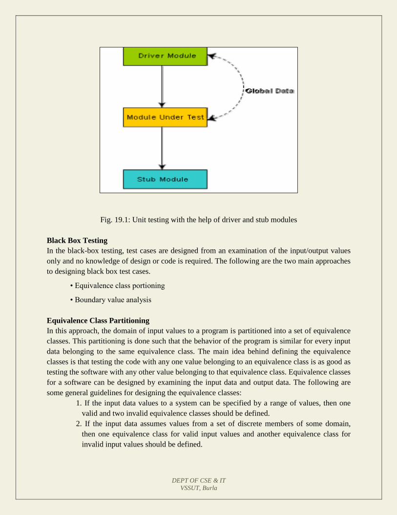
DEPT OF CSE & IT
VSSUT, Burla
Fig. 19.1: Unit testing with the help of driver and stub modules
Black Box Testing
In the black-box testing, test cases are designed from an examination of the input/output values
only and no knowledge of design or code is required. The following are the two main approaches
to designing black box test cases.
• Equivalence class portioning
• Boundary value analysis
Equivalence Class Partitioning
In this approach, the domain of input values to a program is partitioned into a set of equivalence
classes. This partitioning is done such that the behavior of the program is similar for every input
data belonging to the same equivalence class. The main idea behind defining the equivalence
classes is that testing the code with any one value belonging to an equivalence class is as good as
testing the software with any other value belonging to that equivalence class. Equivalence classes
for a software can be designed by examining the input data and output data. The following are
some general guidelines for designing the equivalence classes:
1. If the input data values to a system can be specified by a range of values, then one
valid and two invalid equivalence classes should be defined.
2. If the input data assumes values from a set of discrete members of some domain,
then one equivalence class for valid input values and another equivalence class for
invalid input values should be defined.
DEPT OF CSE & IT
VSSUT, Burla
Example 1: For a software that computes the square root of an input integer which can assume
values in the range of 0 to 5000, there are three equivalence classes: The set of negative integers,
the set of integers in the range of 0 and 5000, and the integers larger than 5000. Therefore, the
test cases must include representatives for each of the three equivalence classes and a possible
test set can be: {-5,500,6000}.
Example 2: Design the black-box test suite for the following program. The program computes
the intersection point of two straight lines and displays the result. It reads two integer pairs (m1,
c1) and (m2, c2) defining the two straight lines of the form y=mx + c.
The equivalence classes are the following:
• Parallel lines (m1=m2, c1≠c2)
• Intersecting lines (m1≠m2)
• Coincident lines (m1=m2, c1=c2)
Now, selecting one representative value from each equivalence class, the test suit (2, 2) (2, 5), (5,
5) (7, 7), (10, 10) (10, 10) are obtained.
Boundary Value Analysis
A type of programming error frequently occurs at the boundaries of different equivalence classes
of inputs. The reason behind such errors might purely be due to psychological factors.
Programmers often fail to see the special processing required by the input values that lie at the
boundary of the different equivalence classes. For example, programmers may improperly use <
instead of <=, or conversely <= for <. Boundary value analysis leads to selection of test cases at
the boundaries of the different equivalence classes.
Example: For a function that computes the square root of integer values in the range of 0 and
5000, the test cases must include the following values: {0, -1,5000,5001}.
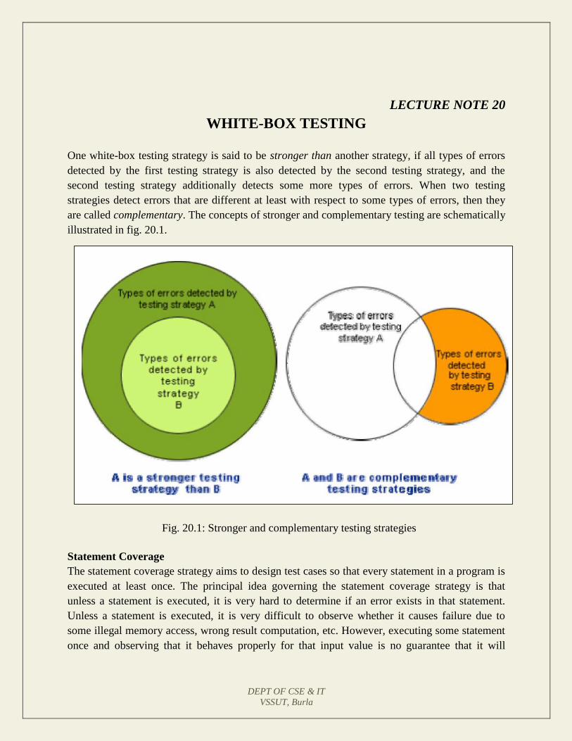
DEPT OF CSE & IT
VSSUT, Burla
LECTURE NOTE 20
WHITE-BOX TESTING
One white-box testing strategy is said to be stronger than another strategy, if all types of errors
detected by the first testing strategy is also detected by the second testing strategy, and the
second testing strategy additionally detects some more types of errors. When two testing
strategies detect errors that are different at least with respect to some types of errors, then they
are called complementary. The concepts of stronger and complementary testing are schematically
illustrated in fig. 20.1.
Fig. 20.1: Stronger and complementary testing strategies
Statement Coverage
The statement coverage strategy aims to design test cases so that every statement in a program is
executed at least once. The principal idea governing the statement coverage strategy is that
unless a statement is executed, it is very hard to determine if an error exists in that statement.
Unless a statement is executed, it is very difficult to observe whether it causes failure due to
some illegal memory access, wrong result computation, etc. However, executing some statement
once and observing that it behaves properly for that input value is no guarantee that it will
DEPT OF CSE & IT
VSSUT, Burla
behave correctly for all input values. In the following, designing of test cases using the statement
coverage strategy have been shown.
Example: Consider the Euclid’s GCD computation algorithm:
int compute_gcd(x, y)
int x, y;
{
1 while (x! = y)
{
2 if (x>y) then
3 x= x – y;
4 else y= y – x;
5 }
6 return x;
}
By choosing the test set {(x=3, y=3), (x=4, y=3), (x=3, y=4)}, we can exercise the program such
that all statements are executed at least once.
Branch Coverage
In the branch coverage-based testing strategy, test cases are designed to make each branch
condition to assume true and false values in turn. Branch testing is also known as edge testing as
in this testing scheme, each edge of a program’s control flow graph is traversed at least once.
It is obvious that branch testing guarantees statement coverage and thus is a stronger testing
strategy compared to the statement coverage-based testing. For Euclid’s GCD computation
algorithm, the test cases for branch coverage can be {(x=3, y=3), (x=3, y=2), (x=4, y=3), (x=3,
y=4)}.
Condition Coverage
In this structural testing, test cases are designed to make each component of a composite
conditional expression to assume both true and false values. For example, in the conditional
expression ((c1.and.c2).or.c3), the components c1, c2 and c3 are each made to assume both true
and false values. Branch testing is probably the simplest condition testing strategy where only
the compound conditions appearing in the different branch statements are made to assume the
true and false values. Thus, condition testing is a stronger testing strategy than branch testing and
branch testing is stronger testing strategy than the statement coverage-based testing. For a
composite conditional expression of n components, for condition coverage, 2ⁿ test cases are
required. Thus, for condition coverage, the number of test cases increases exponentially with the
number of component conditions. Therefore, a condition coverage-based testing technique is
practical only if n (the number of conditions) is small.
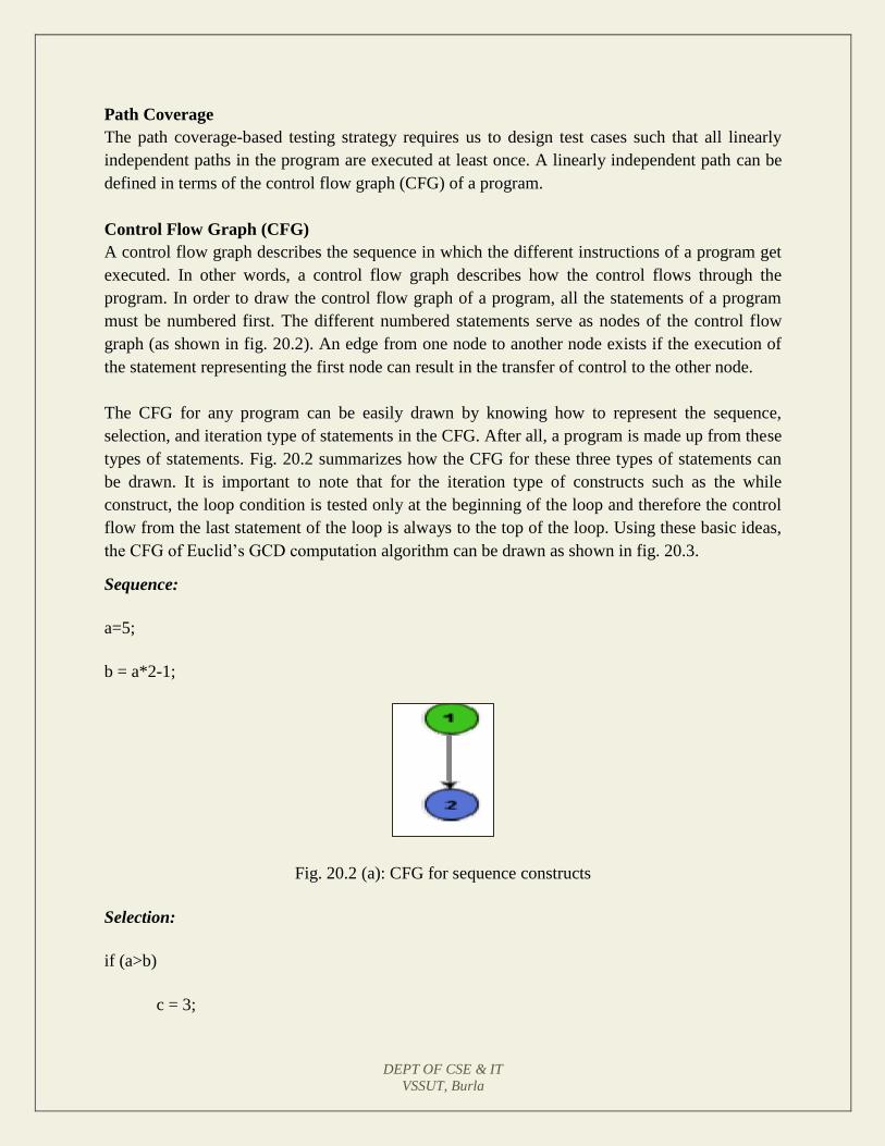
DEPT OF CSE & IT
VSSUT, Burla
Path Coverage
The path coverage-based testing strategy requires us to design test cases such that all linearly
independent paths in the program are executed at least once. A linearly independent path can be
defined in terms of the control flow graph (CFG) of a program.
Control Flow Graph (CFG)
A control flow graph describes the sequence in which the different instructions of a program get
executed. In other words, a control flow graph describes how the control flows through the
program. In order to draw the control flow graph of a program, all the statements of a program
must be numbered first. The different numbered statements serve as nodes of the control flow
graph (as shown in fig. 20.2). An edge from one node to another node exists if the execution of
the statement representing the first node can result in the transfer of control to the other node.
The CFG for any program can be easily drawn by knowing how to represent the sequence,
selection, and iteration type of statements in the CFG. After all, a program is made up from these
types of statements. Fig. 20.2 summarizes how the CFG for these three types of statements can
be drawn. It is important to note that for the iteration type of constructs such as the while
construct, the loop condition is tested only at the beginning of the loop and therefore the control
flow from the last statement of the loop is always to the top of the loop. Using these basic ideas,
the CFG of Euclid’s GCD computation algorithm can be drawn as shown in fig. 20.3.
Sequence:
a=5;
b = a*2-1;
Fig. 20.2 (a): CFG for sequence constructs
Selection:
if (a>b)
c = 3;
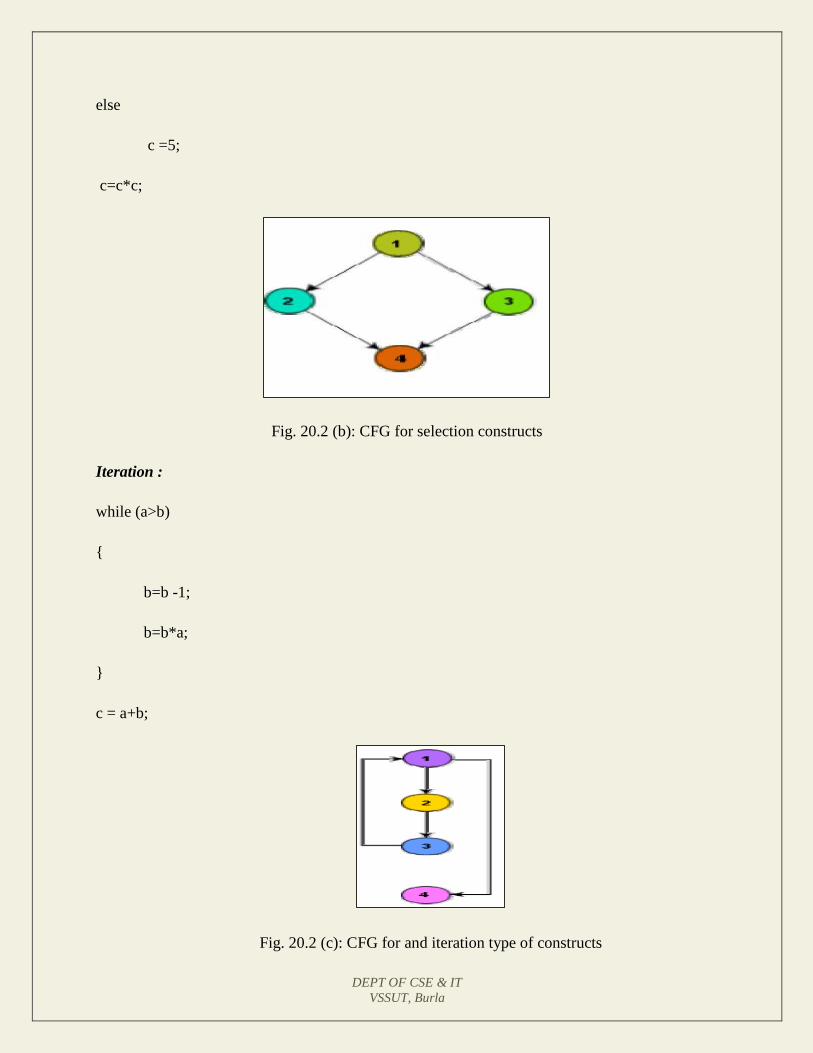
DEPT OF CSE & IT
VSSUT, Burla
else
c =5;
c=c*c;
Fig. 20.2 (b): CFG for selection constructs
Iteration :
while (a>b)
{
b=b -1;
b=b*a;
}
c = a+b;
Fig. 20.2 (c): CFG for and iteration type of constructs
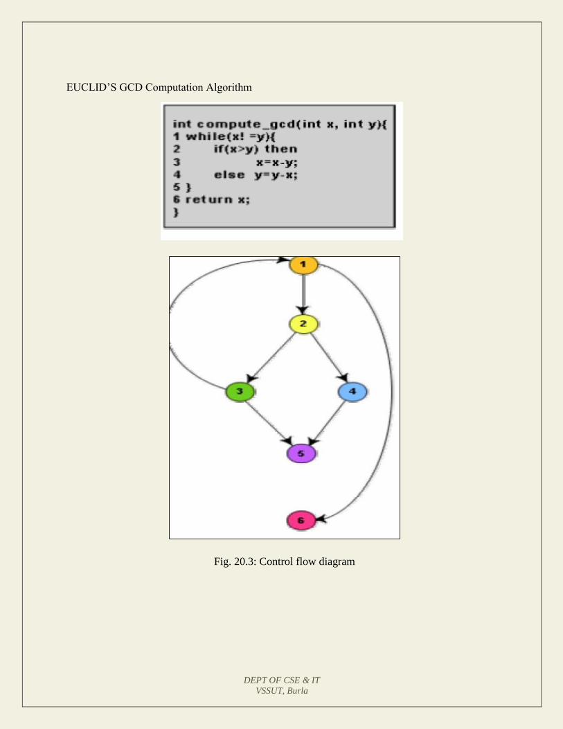
DEPT OF CSE & IT
VSSUT, Burla
EUCLID’S GCD Computation Algorithm
Fig. 20.3: Control flow diagram
DEPT OF CSE & IT
VSSUT, Burla
LECTURE NOTE 21
Path
A path through a program is a node and edge sequence from the starting node to a terminal node
of the control flow graph of a program. There can be more than one terminal node in a program.
Writing test cases to cover all the paths of a typical program is impractical. For this reason, the
path-coverage testing does not require coverage of all paths but only coverage of linearly
independent paths.
Linearly independent path
A linearly independent path is any path through the program that introduces at least one new
edge that is not included in any other linearly independent paths. If a path has one new node
compared to all other linearly independent paths, then the path is also linearly independent. This is
because; any path having a new node automatically implies that it has a new edge. Thus, a path that
is sub-path of another path is not considered to be a linearly independent path.
Control Flow Graph
In order to understand the path coverage-based testing strategy, it is very much necessary to
understand the control flow graph (CFG) of a program. Control flow graph (CFG) of a program has
been discussed earlier.
Linearly Independent Path
The path-coverage testing does not require coverage of all paths but only coverage of linearly
independent paths. Linearly independent paths have been discussed earlier.
Cyclomatic Complexity
For more complicated programs it is not easy to determine the number of independent paths of the
program. McCabe’s cyclomatic complexity defines an upper bound for the number of linearly
independent paths through a program. Also, the McCabe’s cyclomatic complexity is very simple to
compute. Thus, the McCabe’s cyclomatic complexity metric provides a practical way of determining
the maximum number of linearly independent paths in a program. Though the McCabe’s metric does
not directly identify the linearly independent paths, but it informs approximately how many paths to
look for.
There are three different ways to compute the cyclomatic complexity. The answers computed by the
three methods are guaranteed to agree.
DEPT OF CSE & IT
VSSUT, Burla
Method 1:
Given a control flow graph G of a program, the cyclomatic complexity V(G) can be
computed as:
V(G) = E – N + 2
where N is the number of nodes of the control flow graph and E is the number of edges in the
control flow graph.
For the CFG of example shown in fig. 20.3, E=7 and N=6. Therefore, the cyclomatic
complexity = 7-6+2 = 3.
Method 2:
An alternative way of computing the cyclomatic complexity of a program from an inspection
of its control flow graph is as follows:
V(G) = Total number of bounded areas + 1
In the program’s control flow graph G, any region enclosed by nodes and edges can be called
as a bounded area. This is an easy way to determine the McCabe’s cyclomatic complexity.
But, what if the graph G is not planar, i.e. however you draw the graph, two or more edges
intersect? Actually, it can be shown that structured programs always yield planar graphs. But,
presence of GOTO’s can easily add intersecting edges. Therefore, for non-structured
programs, this way of computing the McCabe’s cyclomatic complexity cannot be used.
The number of bounded areas increases with the number of decision paths and loops.
Therefore, the McCabe’s metric provides a quantitative measure of testing difficulty and the
ultimate reliability. For the CFG example shown in fig. 20.3, from a visual examination of
the CFG the number of bounded areas is 2. Therefore the cyclomatic complexity, computing
with this method is also 2+1 = 3. This method provides a very easy way of computing the
cyclomatic complexity of CFGs, just from a visual examination of the CFG. On the other
hand, the other method of computing CFGs is more amenable to automation, i.e. it can be
easily coded into a program which can be used to determine the cyclomatic complexities of
arbitrary CFGs.
Method 3:
The cyclomatic complexity of a program can also be easily computed by computing the
number of decision statements of the program. If N is the number of decision statement of a
program, then the McCabe’s metric is equal to N+1.
DEPT OF CSE & IT
VSSUT, Burla
Data Flow-Based Testing
Data flow-based testing method selects test paths of a program according to the locations of the
definitions and uses of different variables in a program.
For a statement numbered S, let
DEF(S) = {X/statement S contains a definition of X}, and
USES(S) = {X/statement S contains a use of X}
For the statement S:a=b+c;, DEF(S) = {a}. USES(S) = {b,c}. The definition of variable X at
statement S is said to be live at statement S1, if there exists a path from statement S to statement S1
which does not contain any definition of X.
The definition-use chain (or DU chain) of a variable X is of form [X, S, S1], where S and S1 are
statement numbers, such that X Є DEF(S) and X Є USES(S1), and the definition of X in the
statement S is live at statement S1. One simple data flow testing strategy is to require that every DU
chain be covered at least once. Data flow testing strategies are useful for selecting test paths of a
program containing nested if and loop statements.
Mutation Testing
In mutation testing, the software is first tested by using an initial test suite built up from the different
white box testing strategies. After the initial testing is complete, mutation testing is taken up. The
idea behind mutation testing is to make few arbitrary changes to a program at a time. Each time the
program is changed, it is called as a mutated program and the change effected is called as a mutant. A
mutated program is tested against the full test suite of the program. If there exists at least one test
case in the test suite for which a mutant gives an incorrect result, then the mutant is said to be dead. If
a mutant remains alive even after all the test cases have been exhausted, the test data is enhanced to
kill the mutant. The process of generation and killing of mutants can be automated by predefining a
set of primitive changes that can be applied to the program. These primitive changes can be
alterations such as changing an arithmetic operator, changing the value of a constant, changing a data
type, etc. A major disadvantage of the mutation-based testing approach is that it is computationally
very expensive, since a large number of possible mutants can be generated.
Since mutation testing generates a large number of mutants and requires us to check each mutant
with the full test suite, it is not suitable for manual testing. Mutation testing should be used in
conjunction of some testing tool which would run all the test cases automatically.
DEPT OF CSE & IT
VSSUT, Burla
LECTURE NOTE 22
DEBUGGING, INTEGRATION AND SYSTEM TESTING
Need for Debugging
Once errors are identified in a program code, it is necessary to first identify the precise program
statements responsible for the errors and then to fix them. Identifying errors in a program code
and then fix them up are known as debugging.
Debugging Approaches
The following are some of the approaches popularly adopted by programmers for debugging.
Brute Force Method:
This is the most common method of debugging but is the least efficient method. In this
approach, the program is loaded with print statements to print the intermediate values
with the hope that some of the printed values will help to identify the statement in error.
This approach becomes more systematic with the use of a symbolic debugger (also called
a source code debugger), because values of different variables can be easily checked and
break points and watch points can be easily set to test the values of variables effortlessly.
Backtracking:
This is also a fairly common approach. In this approach, beginning from the statement at
which an error symptom has been observed, the source code is traced backwards until the
error is discovered. Unfortunately, as the number of source lines to be traced back
increases, the number of potential backward paths increases and may become
unmanageably large thus limiting the use of this approach.
Cause Elimination Method:
In this approach, a list of causes which could possibly have contributed to the error
symptom is developed and tests are conducted to eliminate each. A related technique of
identification of the error from the error symptom is the software fault tree analysis.
Program Slicing:
This technique is similar to back tracking. Here the search space is reduced by defining
slices. A slice of a program for a particular variable at a particular statement is the set of
source lines preceding this statement that can influence the value of that variable.
DEPT OF CSE & IT
VSSUT, Burla
Debugging Guidelines
Debugging is often carried out by programmers based on their ingenuity. The following are some
general guidelines for effective debugging:
Many times debugging requires a thorough understanding of the program design. Trying
to debug based on a partial understanding of the system design and implementation may
require an inordinate amount of effort to be put into debugging even simple problems.
Debugging may sometimes even require full redesign of the system. In such cases, a
common mistake that novice programmers often make is attempting not to fix the error
but its symptoms.
One must be beware of the possibility that an error correction may introduce new errors.
Therefore after every round of error-fixing, regression testing must be carried out.
Program Analysis Tools
A program analysis tool means an automated tool that takes the source code or the executable
code of a program as input and produces reports regarding several important characteristics of
the program, such as its size, complexity, adequacy of commenting, adherence to programming
standards, etc. We can classify these into two broad categories of program analysis tools:
Static Analysis tools
Dynamic Analysis tools
Static program analysis tools
Static Analysis Tool is also a program analysis tool. It assesses and computes various
characteristics of a software product without executing it. Typically, static analysis tools analyze
some structural representation of a program to arrive at certain analytical conclusions, e.g. that
some structural properties hold. The structural properties that are usually analyzed are:
Whether the coding standards have been adhered to?
Certain programming errors such as uninitialized variables and mismatch
between actual and formal parameters, variables that are declared but never
used are also checked.
Code walk throughs and code inspections might be considered as static analysis methods. But,
the term static program analysis is used to denote automated analysis tools. So, a compiler can be
considered to be a static program analysis tool.
Dynamic program analysis tools - Dynamic program analysis techniques require the program to
be executed and its actual behavior recorded. A dynamic analyzer usually instruments the code
(i.e. adds additional statements in the source code to collect program execution traces). The
instrumented code when executed allows us to record the behavior of the software for different
test cases. After the software has been tested with its full test suite and its behavior recorded, the

DEPT OF CSE & IT
VSSUT, Burla
dynamic analysis tool caries out a post execution analysis and produces reports which describe
the structural coverage that has been achieved by the complete test suite for the program. For
example, the post execution dynamic analysis report might provide data on extent statement,
branch and path coverage achieved.
Normally the dynamic analysis results are reported in the form of a histogram or a pie chart to
describe the structural coverage achieved for different modules of the program. The output of a
dynamic analysis tool can be stored and printed easily and provides evidence that thorough
testing has been done. The dynamic analysis results the extent of testing performed in white-box
mode. If the testing coverage is not satisfactory more test cases can be designed and added to the
test suite. Further, dynamic analysis results can help to eliminate redundant test cases from the
test suite.
DEPT OF CSE & IT
VSSUT, Burla
LECTURE NOTE 23
INTEGRATION TESTING The primary objective of integration testing is to test the module interfaces, i.e. there are no
errors in the parameter passing, when one module invokes another module. During integration
testing, different modules of a system are integrated in a planned manner using an integration
plan. The integration plan specifies the steps and the order in which modules are combined to
realize the full system. After each integration step, the partially integrated system is tested. An
important factor that guides the integration plan is the module dependency graph. The structure
chart (or module dependency graph) denotes the order in which different modules call each
other. By examining the structure chart the integration plan can be developed.
Integration test approaches
There are four types of integration testing approaches. Any one (or a mixture) of the following
approaches can be used to develop the integration test plan. Those approaches are the following:
Big bang approach
Bottom- up approach
Top-down approach
Mixed-approach
Big-Bang Integration Testing
It is the simplest integration testing approach, where all the modules making up a system are
integrated in a single step. In simple words, all the modules of the system are simply put together
and tested. However, this technique is practicable only for very small systems. The main
problem with this approach is that once an error is found during the integration testing, it is very
difficult to localize the error as the error may potentially belong to any of the modules being
integrated. Therefore, debugging errors reported during big bang integration testing are very
expensive to fix.
Bottom-Up Integration Testing
In bottom-up testing, each subsystem is tested separately and then the full system is tested. A
subsystem might consist of many modules which communicate among each other through well-
defined interfaces. The primary purpose of testing each subsystem is to test the interfaces among
various modules making up the subsystem. Both control and data interfaces are tested. The test
cases must be carefully chosen to exercise the interfaces in all possible manners Large software
systems normally require several levels of subsystem testing; lower-level subsystems are
successively combined to form higher-level subsystems. A principal advantage of bottom-up
integration testing is that several disjoint subsystems can be tested simultaneously. In a pure
bottom-up testing no stubs are required, only test-drivers are required. A disadvantage of bottom-
up testing is the complexity that occurs when the system is made up of a large number of small
subsystems. The extreme case corresponds to the big-bang approach.
DEPT OF CSE & IT
VSSUT, Burla
Top-Down Integration Testing
Top-down integration testing starts with the main routine and one or two subordinate routines in
the system. After the top-level ‘skeleton’ has been tested, the immediately subroutines of the
‘skeleton’ are combined with it and tested. Top-down integration testing approach requires the
use of program stubs to simulate the effect of lower-level routines that are called by the routines
under test. A pure top-down integration does not require any driver routines. A disadvantage of
the top-down integration testing approach is that in the absence of lower-level routines, many
times it may become difficult to exercise the top-level routines in the desired manner since the
lower-level routines perform several low-level functions such as I/O.
Mixed Integration Testing
A mixed (also called sandwiched) integration testing follows a combination of top-down and
bottom-up testing approaches. In top-down approach, testing can start only after the top-level
modules have been coded and unit tested. Similarly, bottom-up testing can start only after the
bottom level modules are ready. The mixed approach overcomes this shortcoming of the top-
down and bottom-up approaches. In the mixed testing approaches, testing can start as and when
modules become available. Therefore, this is one of the most commonly used integration testing
approaches.
Phased Vs. Incremental Testing
The different integration testing strategies are either phased or incremental. A comparison of
these two strategies is as follows:
o In incremental integration testing, only one new module is added to the partial
system each time.
o In phased integration, a group of related modules are added to the partial system
each time.
Phased integration requires less number of integration steps compared to the incremental
integration approach. However, when failures are detected, it is easier to debug the system in the
incremental testing approach since it is known that the error is caused by addition of a single
module. In fact, big bang testing is a degenerate case of the phased integration testing approach.
System testing
System tests are designed to validate a fully developed system to assure that it meets its
requirements. There are essentially three main kinds of system testing:
Alpha Testing. Alpha testing refers to the system testing carried out by the test team
within the developing organization.
Beta testing. Beta testing is the system testing performed by a select group of friendly
customers.
Acceptance Testing. Acceptance testing is the system testing performed by the customer
to determine whether he should accept the delivery of the system.
DEPT OF CSE & IT
VSSUT, Burla
In each of the above types of tests, various kinds of test cases are designed by referring to the
SRS document. Broadly, these tests can be classified into functionality and performance tests.
The functionality test tests the functionality of the software to check whether it satisfies the
functional requirements as documented in the SRS document. The performance test tests the
conformance of the system with the nonfunctional requirements of the system.
Performance Testing
Performance testing is carried out to check whether the system needs the non-functional
requirements identified in the SRS document. There are several types of performance testing.
Among of them nine types are discussed below. The types of performance testing to be carried
out on a system depend on the different non-functional requirements of the system documented
in the SRS document. All performance tests can be considered as black-box tests.
• Stress testing
• Volume testing
• Configuration testing
• Compatibility testing
• Regression testing
• Recovery testing
• Maintenance testing
• Documentation testing
• Usability testing
Stress Testing -Stress testing is also known as endurance testing. Stress testing
evaluates system performance when it is stressed for short periods of time. Stress tests are
black box tests which are designed to impose a range of abnormal and even illegal input
conditions so as to stress the capabilities of the software. Input data volume, input data
rate, processing time, utilization of memory, etc. are tested beyond the designed capacity.
For example, suppose an operating system is supposed to support 15 multi programmed
jobs, the system is stressed by attempting to run 15 or more jobs simultaneously. A real-
time system might be tested to determine the effect of simultaneous arrival of several
high-priority interrupts.
Stress testing is especially important for systems that usually operate below the maximum
capacity but are severely stressed at some peak demand hours. For example, if the non-
functional requirement specification states that the response time should not be more than
20 secs per transaction when 60 concurrent users are working, then during the stress
testing the response time is checked with 60 users working simultaneously.
Volume Testing-It is especially important to check whether the data structures (arrays,
queues, stacks, etc.) have been designed to successfully extraordinary situations. For
DEPT OF CSE & IT
VSSUT, Burla
example, a compiler might be tested to check whether the symbol table overflows when a
very large program is compiled.
Configuration Testing - This is used to analyze system behavior in various hardware
and software configurations specified in the requirements. Sometimes systems are built in
variable configurations for different users. For instance, we might define a minimal
system to serve a single user, and other extension configurations to serve additional users.
The system is configured in each of the required configurations and it is checked if the
system behaves correctly in all required configurations.
Compatibility Testing -This type of testing is required when the system interfaces with
other types of systems. Compatibility aims to check whether the interface functions
perform as required. For instance, if the system needs to communicate with a large
database system to retrieve information, compatibility testing is required to test the speed
and accuracy of data retrieval.
Regression Testing -This type of testing is required when the system being tested is an
upgradation of an already existing system to fix some bugs or enhance functionality,
performance, etc. Regression testing is the practice of running an old test suite after each
change to the system or after each bug fix to ensure that no new bug has been introduced
due to the change or the bug fix. However, if only a few statements are changed, then the
entire test suite need not be run - only those test cases that test the functions that are
likely to be affected by the change need to be run.
Recovery Testing -Recovery testing tests the response of the system to the presence of
faults, or loss of power, devices, services, data, etc. The system is subjected to the loss of
the mentioned resources (as applicable and discussed in the SRS document) and it is
checked if the system recovers satisfactorily. For example, the printer can be
disconnected to check if the system hangs. Or, the power may be shut down to check the
extent of data loss and corruption.
Maintenance Testing- This testing addresses the diagnostic programs, and other
procedures that are required to be developed to help maintenance of the system. It is
verified that the artifacts exist and they perform properly.
Documentation Testing- It is checked that the required user manual, maintenance
manuals, and technical manuals exist and are consistent. If the requirements specify the
types of audience for which a specific manual should be designed, then the manual is
checked for compliance.
DEPT OF CSE & IT
VSSUT, Burla
Usability Testing- Usability testing concerns checking the user interface to see if it
meets all user requirements concerning the user interface. During usability testing, the
display screens, report formats, and other aspects relating to the user interface
requirements are tested.
Error Seeding
Sometimes the customer might specify the maximum number of allowable errors that may be
present in the delivered system. These are often expressed in terms of maximum number of
allowable errors per line of source code. Error seed can be used to estimate the number of
residual errors in a system. Error seeding, as the name implies, seeds the code with some known
errors. In other words, some artificial errors are introduced into the program artificially. The
number of these seeded errors detected in the course of the standard testing procedure is
determined. These values in conjunction with the number of unseeded errors detected can be
used to predict:
• The number of errors remaining in the product.
• The effectiveness of the testing strategy.
Let N be the total number of defects in the system and let n of these defects be found by testing.
Let S be the total number of seeded defects, and let s of these defects be found during testing.
n/N = s/S
or
N = S × n/s
Defects still remaining after testing = N–n = n×(S – s)/s
Error seeding works satisfactorily only if the kind of seeded errors matches closely with the kind
of defects that actually exist. However, it is difficult to predict the types of errors that exist in a
software. To some extent, the different categories of errors that remain can be estimated to a first
approximation by analyzing historical data of similar projects. Due to the shortcoming that the
types of seeded errors should match closely with the types of errors actually existing in the code,
error seeding is useful only to a moderate extent.
Regression Testing
Regression testing does not belong to either unit test, integration test, or system testing. Instead,
it is a separate dimension to these three forms of testing. The functionality of regression testing
has been discussed earlier.

DEPT OF CSE & IT
VSSUT, Burla
LECTURE NOTE 24
SOFTWARE MAINTENANCE
Necessity of Software Maintenance
Software maintenance is becoming an important activity of a large number of software
organizations. This is no surprise, given the rate of hardware obsolescence, the immortality of a
software product per se, and the demand of the user community to see the existing software
products run on newer platforms, run in newer environments, and/or with enhanced features.
When the hardware platform is changed, and a software product performs some low-level
functions, maintenance is necessary. Also, whenever the support environment of a software
product changes, the software product requires rework to cope up with the newer interface. For
instance, a software product may need to be maintained when the operating system changes.
Thus, every software product continues to evolve after its development through maintenance
efforts. Therefore it can be stated that software maintenance is needed to correct errors, enhance
features, port the software to new platforms, etc.
Types of software maintenance
There are basically three types of software maintenance. These are:
Corrective: Corrective maintenance of a software product is necessary to rectify the bugs
observed while the system is in use.
Adaptive: A software product might need maintenance when the customers need the
product to run on new platforms, on new operating systems, or when they need the
product to interface with new hardware or software.
Perfective: A software product needs maintenance to support the new features that users
want it to support, to change different functionalities of the system according to customer
demands, or to enhance the performance of the system.
Problems associated with software maintenance
Software maintenance work typically is much more expensive than what it should be and takes
more time than required. In software organizations, maintenance work is mostly carried out
using ad hoc techniques. The primary reason being that software maintenance is one of the most
neglected areas of software engineering. Even though software maintenance is fast becoming an
important area of work for many companies as the software products of yester years age, still
software maintenance is mostly being carried out as fire-fighting operations, rather than through
systematic and planned activities.
Software maintenance has a very poor image in industry. Therefore, an organization often cannot
employ bright engineers to carry out maintenance work. Even though maintenance suffers from a
poor image, the work involved is often more challenging than development work. During
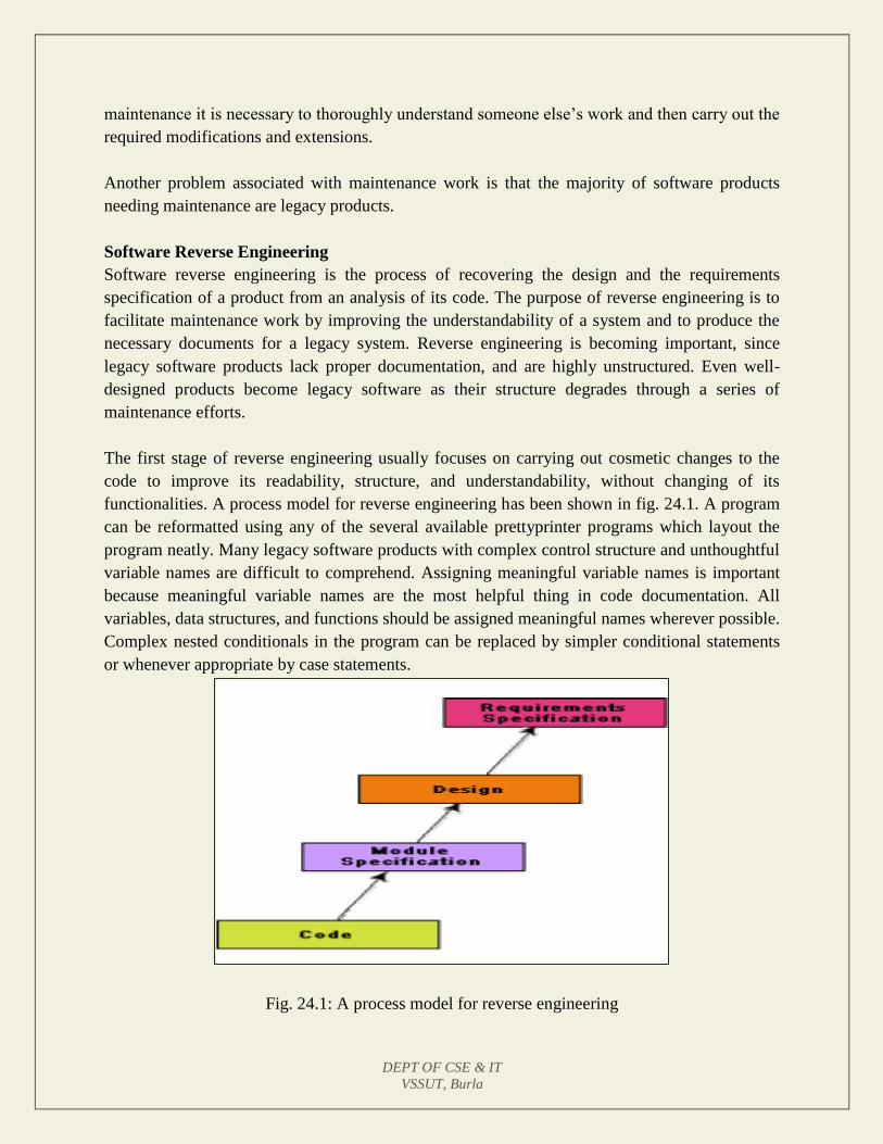
DEPT OF CSE & IT
VSSUT, Burla
maintenance it is necessary to thoroughly understand someone else’s work and then carry out the
required modifications and extensions.
Another problem associated with maintenance work is that the majority of software products
needing maintenance are legacy products.
Software Reverse Engineering
Software reverse engineering is the process of recovering the design and the requirements
specification of a product from an analysis of its code. The purpose of reverse engineering is to
facilitate maintenance work by improving the understandability of a system and to produce the
necessary documents for a legacy system. Reverse engineering is becoming important, since
legacy software products lack proper documentation, and are highly unstructured. Even well-
designed products become legacy software as their structure degrades through a series of
maintenance efforts.
The first stage of reverse engineering usually focuses on carrying out cosmetic changes to the
code to improve its readability, structure, and understandability, without changing of its
functionalities. A process model for reverse engineering has been shown in fig. 24.1. A program
can be reformatted using any of the several available prettyprinter programs which layout the
program neatly. Many legacy software products with complex control structure and unthoughtful
variable names are difficult to comprehend. Assigning meaningful variable names is important
because meaningful variable names are the most helpful thing in code documentation. All
variables, data structures, and functions should be assigned meaningful names wherever possible.
Complex nested conditionals in the program can be replaced by simpler conditional statements
or whenever appropriate by case statements.
Fig. 24.1: A process model for reverse engineering
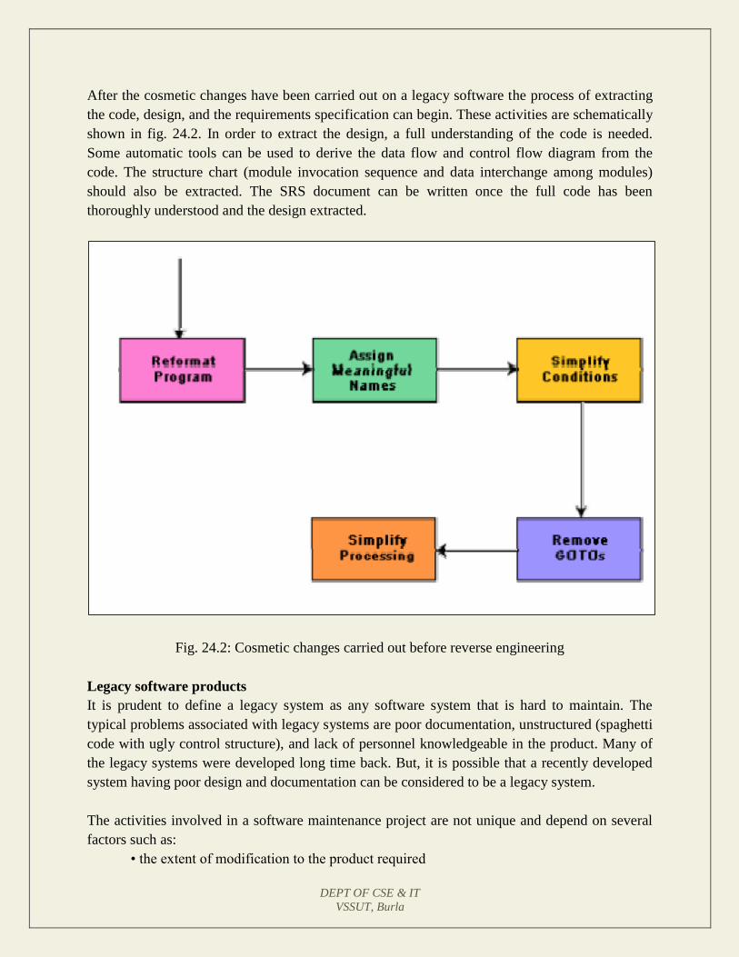
DEPT OF CSE & IT
VSSUT, Burla
After the cosmetic changes have been carried out on a legacy software the process of extracting
the code, design, and the requirements specification can begin. These activities are schematically
shown in fig. 24.2. In order to extract the design, a full understanding of the code is needed.
Some automatic tools can be used to derive the data flow and control flow diagram from the
code. The structure chart (module invocation sequence and data interchange among modules)
should also be extracted. The SRS document can be written once the full code has been
thoroughly understood and the design extracted.
Fig. 24.2: Cosmetic changes carried out before reverse engineering
Legacy software products
It is prudent to define a legacy system as any software system that is hard to maintain. The
typical problems associated with legacy systems are poor documentation, unstructured (spaghetti
code with ugly control structure), and lack of personnel knowledgeable in the product. Many of
the legacy systems were developed long time back. But, it is possible that a recently developed
system having poor design and documentation can be considered to be a legacy system.
The activities involved in a software maintenance project are not unique and depend on several
factors such as:
• the extent of modification to the product required
DEPT OF CSE & IT
VSSUT, Burla
• the resources available to the maintenance team
• the conditions of the existing product (e.g., how structured it is, how well documented it
is, etc.)
• the expected project risks, etc.
When the changes needed to a software product are minor and straightforward, the code can be
directly modified and the changes appropriately reflected in all the documents. But more
elaborate activities are required when the required changes are not so trivial. Usually, for
complex maintenance projects for legacy systems, the software process can be represented by a
reverse engineering cycle followed by a forward engineering cycle with an emphasis on as much
reuse as possible from the existing code and other documents.
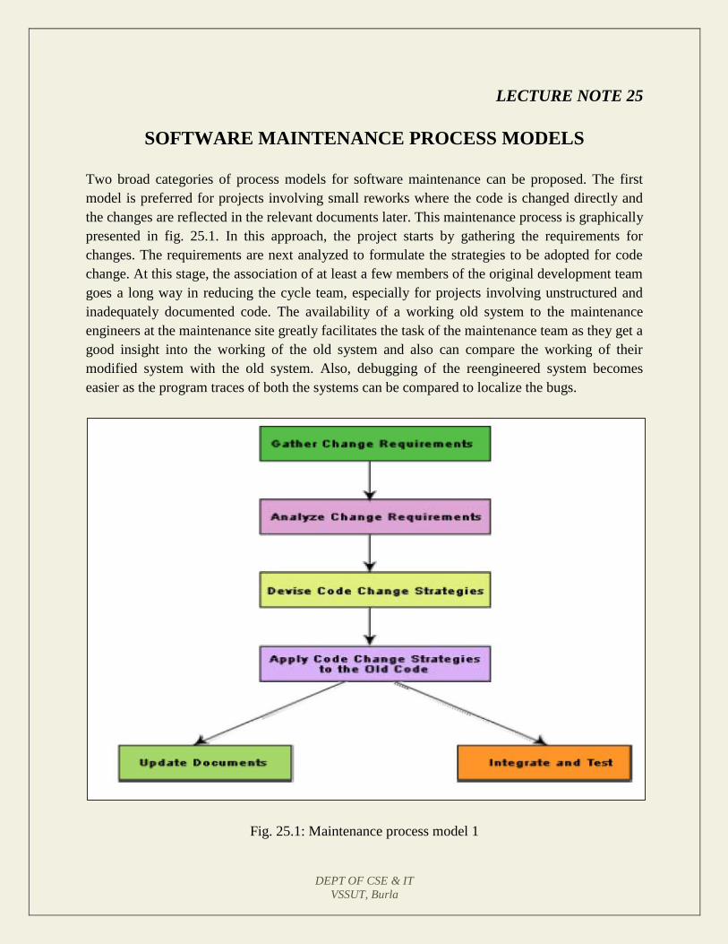
DEPT OF CSE & IT
VSSUT, Burla
LECTURE NOTE 25
SOFTWARE MAINTENANCE PROCESS MODELS
Two broad categories of process models for software maintenance can be proposed. The first
model is preferred for projects involving small reworks where the code is changed directly and
the changes are reflected in the relevant documents later. This maintenance process is graphically
presented in fig. 25.1. In this approach, the project starts by gathering the requirements for
changes. The requirements are next analyzed to formulate the strategies to be adopted for code
change. At this stage, the association of at least a few members of the original development team
goes a long way in reducing the cycle team, especially for projects involving unstructured and
inadequately documented code. The availability of a working old system to the maintenance
engineers at the maintenance site greatly facilitates the task of the maintenance team as they get a
good insight into the working of the old system and also can compare the working of their
modified system with the old system. Also, debugging of the reengineered system becomes
easier as the program traces of both the systems can be compared to localize the bugs.
Fig. 25.1: Maintenance process model 1

DEPT OF CSE & IT
VSSUT, Burla
The second process model for software maintenance is preferred for projects where the amount
of rework required is significant. This approach can be represented by a reverse engineering
cycle followed by a forward engineering cycle. Such an approach is also known as software
reengineering. This process model is depicted in fig. 25.2. The reverse engineering cycle is
required for legacy products. During the reverse engineering, the old code is analyzed
(abstracted) to extract the module specifications. The module specifications are then analyzed to
produce the design. The design is analyzed (abstracted) to produce the original requirements
specification. The change requests are then applied to this requirements specification to arrive at
the new requirements specification. At the design, module specification, and coding a substantial
reuse is made from the reverse engineered products. An important advantage of this approach is
that it produces a more structured design compared to what the original product had, produces
good documentation, and very often results in increased efficiency. The efficiency improvements
are brought about by a more efficient design. However, this approach is more costly than the first
approach. An empirical study indicates that process 1 is preferable when the amount of rework is
no more than 15%. Besides the amount of rework, several other factors might affect the decision
regarding using process model 1 over process model 2:
Reengineering might be preferable for products which exhibit a high failure rate.
Reengineering might also be preferable for legacy products having poor design
and code structure.
Fig. 25.2: Maintenance process model 2
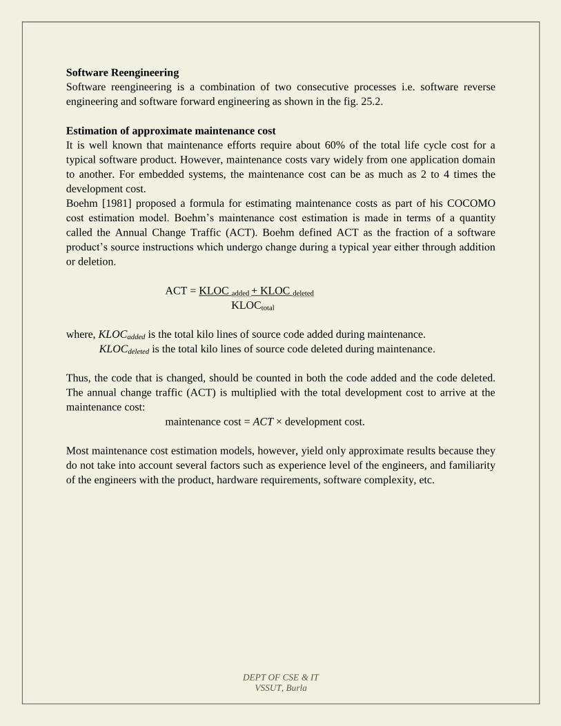
DEPT OF CSE & IT
VSSUT, Burla
Software Reengineering
Software reengineering is a combination of two consecutive processes i.e. software reverse
engineering and software forward engineering as shown in the fig. 25.2.
Estimation of approximate maintenance cost
It is well known that maintenance efforts require about 60% of the total life cycle cost for a
typical software product. However, maintenance costs vary widely from one application domain
to another. For embedded systems, the maintenance cost can be as much as 2 to 4 times the
development cost.
Boehm [1981] proposed a formula for estimating maintenance costs as part of his COCOMO
cost estimation model. Boehm’s maintenance cost estimation is made in terms of a quantity
called the Annual Change Traffic (ACT). Boehm defined ACT as the fraction of a software
product’s source instructions which undergo change during a typical year either through addition
or deletion.
ACT = KLOC added + KLOC deleted
KLOCtotal
where, KLOCadded is the total kilo lines of source code added during maintenance.
KLOCdeleted is the total kilo lines of source code deleted during maintenance.
Thus, the code that is changed, should be counted in both the code added and the code deleted.
The annual change traffic (ACT) is multiplied with the total development cost to arrive at the
maintenance cost:
maintenance cost = ACT × development cost.
Most maintenance cost estimation models, however, yield only approximate results because they
do not take into account several factors such as experience level of the engineers, and familiarity
of the engineers with the product, hardware requirements, software complexity, etc.
DEPT OF CSE & IT
VSSUT, Burla
LECTURE NOTE 26
SOFTWARE RELIABILITY AND QUALITY MANAGEMENT
Repeatable vs. non-repeatable software development organization
A repeatable software development organization is one in which the software development
process is person-independent. In a non-repeatable software development organization, a
software development project becomes successful primarily due to the initiative, effort,
brilliance, or enthusiasm displayed by certain individuals. Thus, in a non-repeatable software
development organization, the chances of successful completion of a software project is to a
great extent depends on the team members.
Software Reliability
Reliability of a software product essentially denotes its trustworthiness or dependability.
Alternatively, reliability of a software product can also be defined as the probability of the
product working “correctly” over a given period of time.
It is obvious that a software product having a large number of defects is unreliable. It is also
clear that the reliability of a system improves, if the number of defects in it is reduced. However,
there is no simple relationship between the observed system reliability and the number of latent
defects in the system. For example, removing errors from parts of a software which are rarely
executed makes little difference to the perceived reliability of the product. It has been
experimentally observed by analyzing the behavior of a large number of programs that 90% of
the execution time of a typical program is spent in executing only 10% of the instructions in the
program. These most used 10% instructions are often called the core of the program. The rest
90% of the program statements are called non-core and are executed only for 10% of the total
execution time. It therefore may not be very surprising to note that removing 60% product
defects from the least used parts of a system would typically lead to only 3% improvement to the
product reliability. It is clear that the quantity by which the overall reliability of a program
improves due to the correction of a single error depends on how frequently the corresponding
instruction is executed.
Thus, reliability of a product depends not only on the number of latent errors but also on the
exact location of the errors. Apart from this, reliability also depends upon how the product is
used, i.e. on its execution profile. If it is selected input data to the system such that only the
“correctly” implemented functions are executed, none of the errors will be exposed and the
perceived reliability of the product will be high. On the other hand, if the input data is selected
such that only those functions which contain errors are invoked, the perceived reliability of the
system will be very low.

DEPT OF CSE & IT
VSSUT, Burla
Reasons for software reliability being difficult to measure
The reasons why software reliability is difficult to measure can be summarized as
follows:
The reliability improvement due to fixing a single bug depends on where the bug is
located in the code.
The perceived reliability of a software product is highly observer-dependent.
The reliability of a product keeps changing as errors are detected and fixed.
Hardware reliability vs. software reliability differs.
Reliability behavior for hardware and software are very different. For example, hardware failures
are inherently different from software failures. Most hardware failures are due to component
wear and tear. A logic gate may be stuck at 1 or 0, or a resistor might short circuit. To fix
hardware faults, one has to either replace or repair the failed part. On the other hand, a software
product would continue to fail until the error is tracked down and either the design or the code is
changed. For this reason, when a hardware is repaired its reliability is maintained at the level that
existed before the failure occurred; whereas when a software failure is repaired, the reliability
may either increase or decrease (reliability may decrease if a bug introduces new errors). To put
this fact in a different perspective, hardware reliability study is concerned with stability (for
example, inter-failure times remain constant). On the other hand, software reliability study aims
at reliability growth (i.e. inter-failure times increase). The change of failure rate over the product
lifetime for a typical hardware and a software product are sketched in fig. 26.1. For hardware
products, it can be observed that failure rate is high initially but decreases as the faulty
components are identified and removed. The system then enters its useful life. After some time
(called product life time) the components wear out, and the failure rate increases. This gives the
plot of hardware reliability over time its characteristics “bath tub” shape. On the other hand, for
software the failure rate is at it’s highest during integration and test. As the system is tested,
more and more errors are identified and removed resulting in reduced failure rate. This error
removal continues at a slower pace during the useful life of the product. As the software
becomes obsolete no error corrections occurs and the failure rate remains unchanged.

DEPT OF CSE & IT
VSSUT, Burla
(a) Hardware product
(b) Software product
Fig. 26.1: Change in failure rate of a product
Reliability Metrics
The reliability requirements for different categories of software products may be different. For
this reason, it is necessary that the level of reliability required for a software product should be
specified in the SRS (software requirements specification) document. In order to be able to do
this, some metrics are needed to quantitatively express the reliability of a software product. A
good reliability measure should be observer-dependent, so that different people can agree on the
degree of reliability a system has. For example, there are precise techniques for measuring
performance, which would result in obtaining the same performance value irrespective of who is
carrying out the performance measurement. However, in practice, it is very difficult to formulate
a precise reliability measurement technique. The next base case is to have measures that correlate
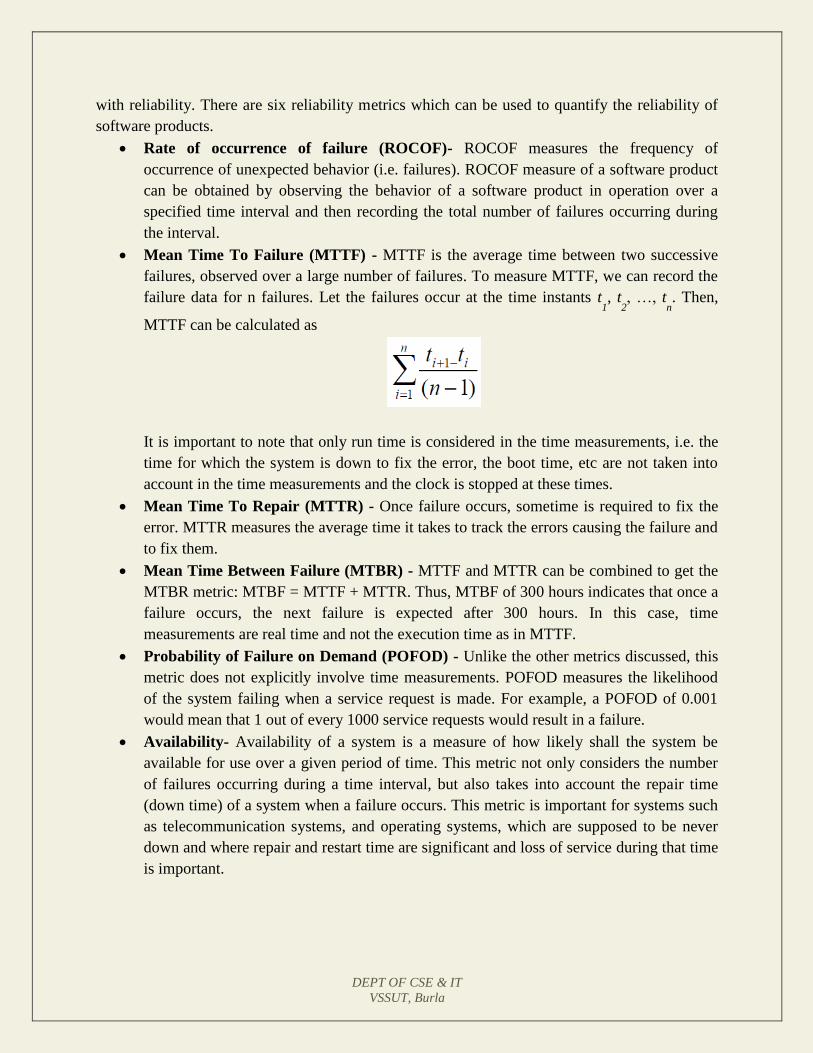
DEPT OF CSE & IT
VSSUT, Burla
with reliability. There are six reliability metrics which can be used to quantify the reliability of
software products.
Rate of occurrence of failure (ROCOF)- ROCOF measures the frequency of
occurrence of unexpected behavior (i.e. failures). ROCOF measure of a software product
can be obtained by observing the behavior of a software product in operation over a
specified time interval and then recording the total number of failures occurring during
the interval.
Mean Time To Failure (MTTF) - MTTF is the average time between two successive
failures, observed over a large number of failures. To measure MTTF, we can record the
failure data for n failures. Let the failures occur at the time instants t1, t
2, …, t
n. Then,
MTTF can be calculated as
It is important to note that only run time is considered in the time measurements, i.e. the
time for which the system is down to fix the error, the boot time, etc are not taken into
account in the time measurements and the clock is stopped at these times.
Mean Time To Repair (MTTR) - Once failure occurs, sometime is required to fix the
error. MTTR measures the average time it takes to track the errors causing the failure and
to fix them.
Mean Time Between Failure (MTBR) - MTTF and MTTR can be combined to get the
MTBR metric: MTBF = MTTF + MTTR. Thus, MTBF of 300 hours indicates that once a
failure occurs, the next failure is expected after 300 hours. In this case, time
measurements are real time and not the execution time as in MTTF.
Probability of Failure on Demand (POFOD) - Unlike the other metrics discussed, this
metric does not explicitly involve time measurements. POFOD measures the likelihood
of the system failing when a service request is made. For example, a POFOD of 0.001
would mean that 1 out of every 1000 service requests would result in a failure.
Availability- Availability of a system is a measure of how likely shall the system be
available for use over a given period of time. This metric not only considers the number
of failures occurring during a time interval, but also takes into account the repair time
(down time) of a system when a failure occurs. This metric is important for systems such
as telecommunication systems, and operating systems, which are supposed to be never
down and where repair and restart time are significant and loss of service during that time
is important.
DEPT OF CSE & IT
VSSUT, Burla
Classification of software failures
A possible classification of failures of software products into five different types is as follows:
Transient- Transient failures occur only for certain input values while invoking a
function of the system.
Permanent- Permanent failures occur for all input values while invoking a function of
the system.
Recoverable- When recoverable failures occur, the system recovers with or without operator
intervention.
Unrecoverable- In unrecoverable failures, the system may need to be restarted.
Cosmetic- These classes of failures cause only minor irritations, and do not lead to
incorrect results. An example of a cosmetic failure is the case where the mouse button has
to be clicked twice instead of once to invoke a given function through the graphical user
interface.
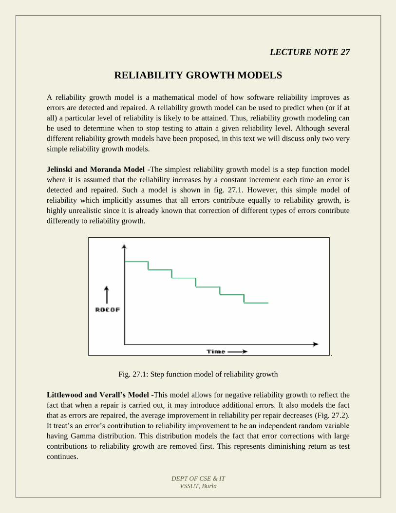
DEPT OF CSE & IT
VSSUT, Burla
LECTURE NOTE 27
RELIABILITY GROWTH MODELS
A reliability growth model is a mathematical model of how software reliability improves as
errors are detected and repaired. A reliability growth model can be used to predict when (or if at
all) a particular level of reliability is likely to be attained. Thus, reliability growth modeling can
be used to determine when to stop testing to attain a given reliability level. Although several
different reliability growth models have been proposed, in this text we will discuss only two very
simple reliability growth models.
Jelinski and Moranda Model -The simplest reliability growth model is a step function model
where it is assumed that the reliability increases by a constant increment each time an error is
detected and repaired. Such a model is shown in fig. 27.1. However, this simple model of
reliability which implicitly assumes that all errors contribute equally to reliability growth, is
highly unrealistic since it is already known that correction of different types of errors contribute
differently to reliability growth.
.
Fig. 27.1: Step function model of reliability growth
Littlewood and Verall’s Model -This model allows for negative reliability growth to reflect the
fact that when a repair is carried out, it may introduce additional errors. It also models the fact
that as errors are repaired, the average improvement in reliability per repair decreases (Fig. 27.2).
It treat’s an error’s contribution to reliability improvement to be an independent random variable
having Gamma distribution. This distribution models the fact that error corrections with large
contributions to reliability growth are removed first. This represents diminishing return as test
continues.
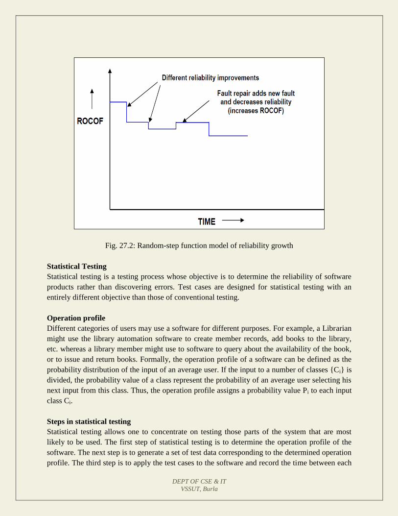
DEPT OF CSE & IT
VSSUT, Burla
Fig. 27.2: Random-step function model of reliability growth
Statistical Testing
Statistical testing is a testing process whose objective is to determine the reliability of software
products rather than discovering errors. Test cases are designed for statistical testing with an
entirely different objective than those of conventional testing.
Operation profile
Different categories of users may use a software for different purposes. For example, a Librarian
might use the library automation software to create member records, add books to the library,
etc. whereas a library member might use to software to query about the availability of the book,
or to issue and return books. Formally, the operation profile of a software can be defined as the
probability distribution of the input of an average user. If the input to a number of classes {Ci} is
divided, the probability value of a class represent the probability of an average user selecting his
next input from this class. Thus, the operation profile assigns a probability value Pi to each input
class Ci.
Steps in statistical testing
Statistical testing allows one to concentrate on testing those parts of the system that are most
likely to be used. The first step of statistical testing is to determine the operation profile of the
software. The next step is to generate a set of test data corresponding to the determined operation
profile. The third step is to apply the test cases to the software and record the time between each

DEPT OF CSE & IT
VSSUT, Burla
failure. After a statistically significant number of failures have been observed, the reliability can
be computed.
Advantages and disadvantages of statistical testing
Statistical testing allows one to concentrate on testing parts of the system that are most likely to
be used. Therefore, it results in a system that the users to be more reliable (than actually it is!).
Reliability estimation using statistical testing is more accurate compared to those of other
methods such as ROCOF, POFOD etc. But it is not easy to perform statistical testing properly.
There is no simple and repeatable way of defining operation profiles. Also it is very much
cumbersome to generate test cases for statistical testing because the number of test cases with
which the system is to be tested should be statistically significant.
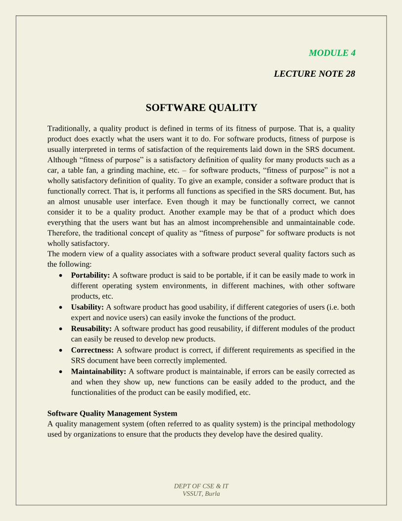
DEPT OF CSE & IT
VSSUT, Burla
MODULE 4
LECTURE NOTE 28
SOFTWARE QUALITY
Traditionally, a quality product is defined in terms of its fitness of purpose. That is, a quality
product does exactly what the users want it to do. For software products, fitness of purpose is
usually interpreted in terms of satisfaction of the requirements laid down in the SRS document.
Although “fitness of purpose” is a satisfactory definition of quality for many products such as a
car, a table fan, a grinding machine, etc. – for software products, “fitness of purpose” is not a
wholly satisfactory definition of quality. To give an example, consider a software product that is
functionally correct. That is, it performs all functions as specified in the SRS document. But, has
an almost unusable user interface. Even though it may be functionally correct, we cannot
consider it to be a quality product. Another example may be that of a product which does
everything that the users want but has an almost incomprehensible and unmaintainable code.
Therefore, the traditional concept of quality as “fitness of purpose” for software products is not
wholly satisfactory.
The modern view of a quality associates with a software product several quality factors such as
the following:
Portability: A software product is said to be portable, if it can be easily made to work in
different operating system environments, in different machines, with other software
products, etc.
Usability: A software product has good usability, if different categories of users (i.e. both
expert and novice users) can easily invoke the functions of the product.
Reusability: A software product has good reusability, if different modules of the product
can easily be reused to develop new products.
Correctness: A software product is correct, if different requirements as specified in the
SRS document have been correctly implemented.
Maintainability: A software product is maintainable, if errors can be easily corrected as
and when they show up, new functions can be easily added to the product, and the
functionalities of the product can be easily modified, etc.
Software Quality Management System
A quality management system (often referred to as quality system) is the principal methodology
used by organizations to ensure that the products they develop have the desired quality.

DEPT OF CSE & IT
VSSUT, Burla
A quality system consists of the following:
Managerial Structure and Individual Responsibilities- A quality system is actually the
responsibility of the organization as a whole. However, every organization has a separate quality
department to perform several quality system activities. The quality system of an organization
should have support of the top management. Without support for the quality system at a high
level in a company, few members of staff will take the quality system seriously.
Quality System Activities- The quality system activities encompass the following:
- auditing of projects
- review of the quality system
- development of standards, procedures, and guidelines, etc.
- production of reports for the top management summarizing the effectiveness of the
quality system in the organization.
Evolution of Quality Management System
Quality systems have rapidly evolved over the last five decades. Prior to World War II, the usual
method to produce quality products was to inspect the finished products to eliminate defective
products. Since that time, quality systems of organizations have undergone through four stages
of evolution as shown in the fig. 28.1. The initial product inspection method gave way to quality
control (QC). Quality control focuses not only on detecting the defective products and
eliminating them but also on determining the causes behind the defects. Thus, quality control
aims at correcting the causes of errors and not just rejecting the products. The next breakthrough
in quality systems was the development of quality assurance principles.
The basic premise of modern quality assurance is that if an organization’s processes are good
and are followed rigorously, then the products are bound to be of good quality. The modern
quality paradigm includes guidance for recognizing, defining, analyzing, and improving the
production process. Total quality management (TQM) advocates that the process followed by an
organization must be continuously improved through process measurements. TQM goes a step
further than quality assurance and aims at continuous process improvement. TQM goes beyond
documenting processes to optimizing them through redesign. A term related to TQM is Business
Process Reengineering (BPR). BPR aims at reengineering the way business is carried out in an
organization. From the above discussion it can be stated that over the years the quality paradigm
has shifted from product assurance to process assurance (as shown in fig. 28.1).
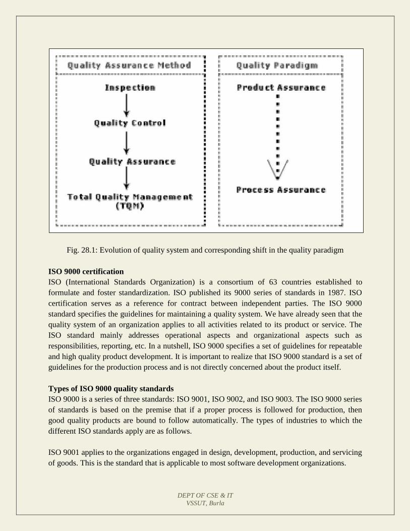
DEPT OF CSE & IT
VSSUT, Burla
Fig. 28.1: Evolution of quality system and corresponding shift in the quality paradigm
ISO 9000 certification
ISO (International Standards Organization) is a consortium of 63 countries established to
formulate and foster standardization. ISO published its 9000 series of standards in 1987. ISO
certification serves as a reference for contract between independent parties. The ISO 9000
standard specifies the guidelines for maintaining a quality system. We have already seen that the
quality system of an organization applies to all activities related to its product or service. The
ISO standard mainly addresses operational aspects and organizational aspects such as
responsibilities, reporting, etc. In a nutshell, ISO 9000 specifies a set of guidelines for repeatable
and high quality product development. It is important to realize that ISO 9000 standard is a set of
guidelines for the production process and is not directly concerned about the product itself.
Types of ISO 9000 quality standards
ISO 9000 is a series of three standards: ISO 9001, ISO 9002, and ISO 9003. The ISO 9000 series
of standards is based on the premise that if a proper process is followed for production, then
good quality products are bound to follow automatically. The types of industries to which the
different ISO standards apply are as follows.
ISO 9001 applies to the organizations engaged in design, development, production, and servicing
of goods. This is the standard that is applicable to most software development organizations.
DEPT OF CSE & IT
VSSUT, Burla
ISO 9002 applies to those organizations which do not design products but are only involved in
production. Examples of these category industries include steel and car manufacturing industries
that buy the product and plant designs from external sources and are involved in only
manufacturing those products. Therefore, ISO 9002 is not applicable to software development
organizations.
ISO 9003 applies to organizations that are involved only in installation and testing of the
products.
Software products vs. other products
There are mainly two differences between software products and any other type of products.
Software is intangible in nature and therefore difficult to control. It is very difficult to
control and manage anything that is not seen. In contrast, any other industries such as car
manufacturing industries where one can see a product being developed through various
stages such as fitting engine, fitting doors, etc. Therefore, it is easy to accurately
determine how much work has been completed and to estimate how much more time will
it take.
During software development, the only raw material consumed is data. In contrast, large
quantities of raw materials are consumed during the development of any other product.
Need for obtaining ISO 9000 certification
There is a mad scramble among software development organizations for obtaining ISO
certification due to the benefits it offers. Some benefits that can be acquired to organizations by
obtaining ISO certification are as follows:
Confidence of customers in an organization increases when organization qualifies for
ISO certification. This is especially true in the international market. In fact, many
organizations awarding international software development contracts insist that the
development organization have ISO 9000 certification. For this reason, it is vital for
software organizations involved in software export to obtain ISO 9000 certification.
ISO 9000 requires a well-documented software production process to be in place. A well-
documented software production process contributes to repeatable and higher quality of
the developed software.
ISO 9000 makes the development process focused, efficient, and cost-effective.
ISO 9000 certification points out the weak points of an organization and recommends
remedial action.
ISO 9000 sets the basic framework for the development of an optimal process and Total
Quality Management (TQM).
DEPT OF CSE & IT
VSSUT, Burla
Summary of ISO 9001 certification
A summary of the main requirements of ISO 9001 as they relate of software development is as
follows. Section numbers in brackets correspond to those in the standard itself:
Management Responsibility (4.1)
The management must have an effective quality policy.
The responsibility and authority of all those whose work affects quality must be defined
and documented.
A management representative, independent of the development process, must be
responsible for the quality system. This requirement probably has been put down so that
the person responsible for the quality system can work in an unbiased manner.
The effectiveness of the quality system must be periodically reviewed by audits.
Quality System (4.2)
A quality system must be maintained and documented.
Contract Reviews (4.3)
Before entering into a contract, an organization must review the contract to ensure that it is
understood, and that the organization has the necessary capability for carrying out its obligations.
Design Control (4.4)
The design process must be properly controlled, this includes controlling coding also.
This requirement means that a good configuration control system must be in place.
Design inputs must be verified as adequate.
Design must be verified.
Design output must be of required quality.
Design changes must be controlled.
Document Control (4.5)
There must be proper procedures for document approval, issue and removal.
Document changes must be controlled. Thus, use of some configuration management
tools is necessary.
Purchasing (4.6)
Purchasing material, including bought-in software must be checked for conforming to
requirements.
Purchaser Supplied Product (4.7)
Material supplied by a purchaser, for example, client-provided software must be properly
managed and checked.
DEPT OF CSE & IT
VSSUT, Burla
Product Identification (4.8)
The product must be identifiable at all stages of the process. In software terms this means
configuration management.
Process Control (4.9)
The development must be properly managed.
Quality requirement must be identified in a quality plan.
Inspection and Testing (4.10)
In software terms this requires effective testing i.e., unit testing, integration testing and system
testing. Test records must be maintained.
Inspection, Measuring and Test Equipment (4.11)
If integration, measuring, and test equipments are used, they must be properly maintained and
calibrated.
Inspection and Test Status (4.12)
The status of an item must be identified. In software terms this implies configuration
management and release control.
Control of Nonconforming Product (4.13)
In software terms, this means keeping untested or faulty software out of the released product, or
other places whether it might cause damage.
Corrective Action (4.14)
This requirement is both about correcting errors when found, and also investigating why the
errors occurred and improving the process to prevent occurrences. If an error occurs despite the
quality system, the system needs improvement.
Handling, (4.15)
This clause deals with the storage, packing, and delivery of the software product.
Quality records (4.16)
Recording the steps taken to control the quality of the process is essential in order to be able to
confirm that they have actually taken place.
Quality Audits (4.17)
Audits of the quality system must be carried out to ensure that it is effective.

DEPT OF CSE & IT
VSSUT, Burla
Training (4.18)
Training needs must be identified and met.
Salient features of ISO 9001 certification
The salient features of ISO 9001 are as follows:
All documents concerned with the development of a software product should be properly
managed, authorized, and controlled. This requires a configuration management system
to be in place.
Proper plans should be prepared and then progress against these plans should be
monitored.
Important documents should be independently checked and reviewed for effectiveness
and correctness.
The product should be tested against specification.
Several organizational aspects should be addressed e.g., management reporting of the
quality team.
Shortcomings of ISO 9000 certification
Even though ISO 9000 aims at setting up an effective quality system in an organization, it suffers
from several shortcomings. Some of these shortcomings of the ISO 9000 certification process are
the following:
ISO 9000 requires a software production process to be adhered to but does not guarantee
the process to be of high quality. It also does not give any guideline for defining an
appropriate process.
ISO 9000 certification process is not fool-proof and no international accreditation agency
exists. Therefore it is likely that variations in the norms of awarding certificates can exist
among the different accreditation agencies and also among the registrars.
Organizations getting ISO 9000 certification often tend to downplay domain expertise.
These organizations start to believe that since a good process is in place, any engineer is
as effective as any other engineer in doing any particular activity relating to software
development. However, many areas of software development are so specialized that
special expertise and experience in these areas (domain expertise) is required. In
manufacturing industry there is a clear link between process quality and product quality.
Once a process is calibrated, it can be run again and again producing quality goods. In
contrast, software development is a creative process and individual skills and experience
are important.
ISO 9000 does not automatically lead to continuous process improvement, i.e. does not
automatically lead to TQM.
DEPT OF CSE & IT
VSSUT, Burla
LECTURE NOTE 29
SEI CAPABILITY MATURITY MODEL
SEI Capability Maturity Model (SEI CMM) helped organizations to improve the quality of the
software they develop and therefore adoption of SEI CMM model has significant business
benefits.
SEI CMM can be used two ways: capability evaluation and software process assessment.
Capability evaluation and software process assessment differ in motivation, objective, and the
final use of the result. Capability evaluation provides a way to assess the software process
capability of an organization. The results of capability evaluation indicates the likely contractor
performance if the contractor is awarded a work. Therefore, the results of software process
capability assessment can be used to select a contractor. On the other hand, software process
assessment is used by an organization with the objective to improve its process capability. Thus,
this type of assessment is for purely internal use.
SEI CMM classifies software development industries into the following five maturity levels. The
different levels of SEI CMM have been designed so that it is easy for an organization to slowly
build its quality system starting from scratch.
Level 1: Initial - A software development organization at this level is characterized by ad hoc
activities. Very few or no processes are defined and followed. Since software production
processes are not defined, different engineers follow their own process and as a result
development efforts become chaotic. Therefore, it is also called chaotic level. The success of
projects depends on individual efforts and heroics. When engineers leave, the successors have
great difficulty in understanding the process followed and the work completed. Since formal
project management practices are not followed, under time pressure short cuts are tried out
leading to low quality.
Level 2: Repeatable - At this level, the basic project management practices such as tracking cost
and schedule are established. Size and cost estimation techniques like function point analysis,
COCOMO, etc. are used. The necessary process discipline is in place to repeat earlier success on
projects with similar applications. Please remember that opportunity to repeat a process exists
only when a company produces a family of products.
Level 3: Defined - At this level the processes for both management and development activities
are defined and documented. There is a common organization-wide understanding of activities,
roles, and responsibilities. The processes though defined, the process and product qualities are
not measured. ISO 9000 aims at achieving this level.
DEPT OF CSE & IT
VSSUT, Burla
Level 4: Managed - At this level, the focus is on software metrics. Two types of metrics are
collected. Product metrics measure the characteristics of the product being developed, such as its
size, reliability, time complexity, understandability, etc. Process metrics reflect the effectiveness
of the process being used, such as average defect correction time, productivity, average number
of defects found per hour inspection, average number of failures detected during testing per
LOC, etc. Quantitative quality goals are set for the products. The software process and product
quality are measured and quantitative quality requirements for the product are met. Various tools
like Pareto charts, fishbone diagrams, etc. are used to measure the product and process quality.
The process metrics are used to check if a project performed satisfactorily. Thus, the results of
process measurements are used to evaluate project performance rather than improve the process.
Level 5: Optimizing - At this stage, process and product metrics are collected. Process and
product measurement data are analyzed for continuous process improvement. For example, if
from an analysis of the process measurement results, it was found that the code reviews were not
very effective and a large number of errors were detected only during the unit testing, then the
process may be fine-tuned to make the review more effective. Also, the lessons learned from
specific projects are incorporated in to the process. Continuous process improvement is achieved
both by carefully analyzing the quantitative feedback from the process measurements and also
from application of innovative ideas and technologies. Such an organization identifies the best
software engineering practices and innovations which may be tools, methods, or processes.
These best practices are transferred throughout the organization.
Key process areas (KPA) of a software organization
Except for SEI CMM level 1, each maturity level is characterized by several Key Process Areas
(KPAs) that includes the areas an organization should focus to improve its software process to
the next level. The focus of each level and the corresponding key process areas are shown in the
fig. 29.1.

DEPT OF CSE & IT
VSSUT, Burla
CMM Level Focus Key Process Ares
1. Initial Competent people
2. Repeatable Project management Software project planning
Software configuration management
3. Defined Definition of processes Process definition
Training program
Peer reviews
4. Managed Product and process
quality
Quantitative process metrics
Software quality management
5. Optimizing Continuous process
improvement
Defect prevention
Process change management
Technology change management
Fig. 29.1: The focus of each SEI CMM level and the corresponding key process areas
SEI CMM provides a list of key areas on which to focus to take an organization from one level
of maturity to the next. Thus, it provides a way for gradual quality improvement over several
stages. Each stage has been carefully designed such that one stage enhances the capability
already built up. For example, it considers that trying to implement a defined process (SEI CMM
level 3) before a repeatable process (SEI CMM level 2) would be counterproductive as it
becomes difficult to follow the defined process due to schedule and budget pressures. ISO 9000
certification vs. SEI/CMM
For quality appraisal of a software development organization, the characteristics of ISO 9000
certification and the SEI CMM differ in some respects. The differences are as follows:
ISO 9000 is awarded by an international standards body. Therefore, ISO 9000
certification can be quoted by an organization in official documents, communication with
external parties, and the tender quotations. However, SEI CMM assessment is purely for
internal use.
SEI CMM was developed specifically for software industry and therefore addresses many
issues which are specific to software industry alone.
SEI CMM goes beyond quality assurance and prepares an organization to ultimately
achieve Total Quality Management (TQM). In fact, ISO 9001 aims at level 3 of SEI
CMM model.
SEI CMM model provides a list of key process areas (KPAs) on which an organization at
any maturity level needs to concentrate to take it from one maturity level to the next.
Thus, it provides a way for achieving gradual quality improvement.
DEPT OF CSE & IT
VSSUT, Burla
Applicability of SEI CMM to organizations
Highly systematic and measured approach to software development suits large organizations
dealing with negotiated software, safety-critical software, etc. For those large organizations, SEI
CMM model is perfectly applicable. But small organizations typically handle applications such
as Internet, e-commerce, and are without an established product range, revenue base, and
experience on past projects, etc. For such organizations, a CMM-based appraisal is probably
excessive. These organizations need to operate more efficiently at the lower levels of maturity.
For example, they need to practice effective project management, reviews, configuration
management, etc.
Personal Software Process
Personal Software Process (PSP) is a scaled down version of the industrial software process. PSP
is suitable for individual use. It is important to note that SEI CMM does not tell software
developers how to analyze, design, code, test, or document software products, but assumes that
engineers use effective personal practices. PSP recognizes that the process for individual use is
different from that necessary for a team.
The quality and productivity of an engineer is to a great extent dependent on his process. PSP is
a framework that helps engineers to measure and improve the way they work. It helps in
developing personal skills and methods by estimating and planning, by showing how to track
performance against plans, and provides a defined process which can be tuned by individuals.
Time measurement- PSP advocates that engineers should rack the way they spend time.
Because, boring activities seem longer than actual and interesting activities seem short.
Therefore, the actual time spent on a task should be measured with the help of a stop-clock to get
an objective picture of the time spent. For example, he may stop the clock when attending a
telephone call, taking a coffee break etc. An engineer should measure the time he spends for
designing, writing code, testing, etc.
PSP Planning- Individuals must plan their project. They must estimate the maximum, minimum,
and the average LOC required for the product. They should use their productivity in
minutes/LOC to calculate the maximum, minimum, and the average development time. They
must record the plan data in a project plan summary.
The PSP is schematically shown in fig. 29.2. While carrying out the different phases, they must
record the log data using time measurement. During post-mortem, they can compare the log data
with their project plan to achieve better planning in the future projects, to improve their process,
etc.
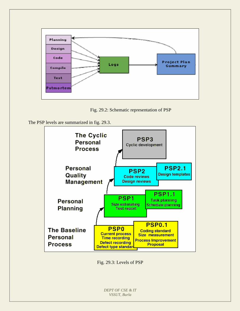
DEPT OF CSE & IT
VSSUT, Burla
Fig. 29.2: Schematic representation of PSP
The PSP levels are summarized in fig. 29.3.
Fig. 29.3: Levels of PSP
DEPT OF CSE & IT
VSSUT, Burla
PSP2 introduces defect management via the use of checklists for code and design reviews. The
checklists are developed from gathering and analyzing defect data earlier projects.
Six Sigma
The purpose of Six Sigma is to improve processes to do things better, faster, and at lower cost. It
can be used to improve every facet of business, from production, to human resources, to order
entry, to technical support. Six Sigma can be used for any activity that is concerned with cost,
timeliness, and quality of results. Therefore, it is applicable to virtually every industry.
Six Sigma at many organizations simply means striving for near perfection. Six Sigma is a
disciplined, data-driven approach to eliminate defects in any process – from manufacturing to
transactional and product to service.
The statistical representation of Six Sigma describes quantitatively how a process is performing.
To achieve Six Sigma, a process must not produce more than 3.4 defects per million
opportunities. A Six Sigma defect is defined as any system behavior that is not as per customer
specifications. Total number of Six Sigma opportunities is then the total number of chances for a
defect. Process sigma can easily be calculated using a Six Sigma calculator.
The fundamental objective of the Six Sigma methodology is the implementation of a
measurement-based strategy that focuses on process improvement and variation reduction
through the application of Six Sigma improvement projects. This is accomplished through the
use of two Six Sigma sub-methodologies: DMAIC and DMADV. The Six Sigma DMAIC
process (define, measure, analyze, improve, control) is an improvement system for existing
processes failing below specification and looking for incremental improvement. The Six Sigma
DMADV process (define, measure, analyze, design, verify) is an improvement system used to
develop new processes or products at Six Sigma quality levels. It can also be employed if a
current process requires more than just incremental improvement. Both Six Sigma processes are
executed by Six Sigma Green Belts and Six Sigma Black Belts, and are overseen by Six Sigma
Master Black Belts.
Many frameworks exist for implementing the Six Sigma methodology. Six Sigma Consultants
all over the world have also developed proprietary methodologies for implementing Six Sigma
quality, based on the similar change management philosophies and applications of tools.

DEPT OF CSE & IT
VSSUT, Burla
LECTURE NOTE 30
SOFTWARE PROJECT PLANNING
Project Planning and Project Estimation Techniques
Responsibilities of a software project manager
Software project managers take the overall responsibility of steering a project to success. It is
very difficult to objectively describe the job responsibilities of a project manager. The job
responsibility of a project manager ranges from invisible activities like building up team morale
to highly visible customer presentations. Most managers take responsibility for project proposal
writing, project cost estimation, scheduling, project staffing, software process tailoring, project
monitoring and control, software configuration management, risk management, interfacing with
clients, managerial report writing and presentations, etc. These activities are certainly numerous,
varied and difficult to enumerate, but these activities can be broadly classified into project
planning, and project monitoring and control activities. The project planning activity is
undertaken before the development starts to plan the activities to be undertaken during
development. The project monitoring and control activities are undertaken once the development
activities start with the aim of ensuring that the development proceeds as per plan and changing
the plan whenever required to cope up with the situation.
Skills necessary for software project management
A theoretical knowledge of different project management techniques is certainly necessary to
become a successful project manager. However, effective software project management
frequently calls for good qualitative judgment and decision taking capabilities. In addition to
having a good grasp of the latest software project management techniques such as cost
estimation, risk management, configuration management, project managers need good
communication skills and the ability get work done. However, some skills such as tracking and
controlling the progress of the project, customer interaction, managerial presentations, and team
building are largely acquired through experience. None the less, the importance of sound
knowledge of the prevalent project management techniques cannot be overemphasized.
Project Planning
Once a project is found to be feasible, software project managers undertake project planning.
Project planning is undertaken and completed even before any development activity starts.
Project planning consists of the following essential activities:
Estimating the following attributes of the project:
Project size: What will be problem complexity in terms of the effort and time
required to develop the product?
Cost: How much is it going to cost to develop the project?
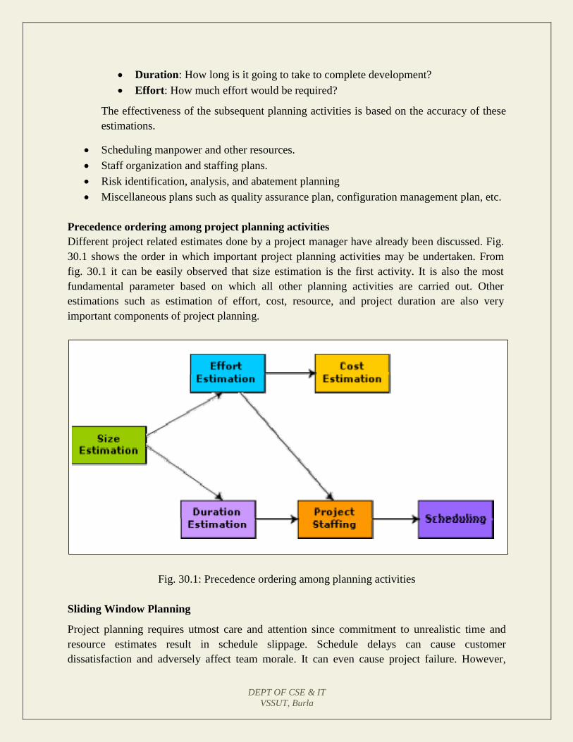
DEPT OF CSE & IT
VSSUT, Burla
Duration: How long is it going to take to complete development?
Effort: How much effort would be required?
The effectiveness of the subsequent planning activities is based on the accuracy of these
estimations.
Scheduling manpower and other resources.
Staff organization and staffing plans.
Risk identification, analysis, and abatement planning
Miscellaneous plans such as quality assurance plan, configuration management plan, etc.
Precedence ordering among project planning activities
Different project related estimates done by a project manager have already been discussed. Fig.
30.1 shows the order in which important project planning activities may be undertaken. From
fig. 30.1 it can be easily observed that size estimation is the first activity. It is also the most
fundamental parameter based on which all other planning activities are carried out. Other
estimations such as estimation of effort, cost, resource, and project duration are also very
important components of project planning.
Fig. 30.1: Precedence ordering among planning activities
Sliding Window Planning
Project planning requires utmost care and attention since commitment to unrealistic time and
resource estimates result in schedule slippage. Schedule delays can cause customer
dissatisfaction and adversely affect team morale. It can even cause project failure. However,

DEPT OF CSE & IT
VSSUT, Burla
project planning is a very challenging activity. Especially for large projects, it is very much
difficult to make accurate plans. A part of this difficulty is due to the fact that the proper
parameters, scope of the project, project staff, etc. may change during the span of the project. In
order to overcome this problem, sometimes project managers undertake project planning in
stages. Planning a project over a number of stages protects managers from making big
commitments too early. This technique of staggered planning is known as Sliding Window
Planning. In the sliding window technique, starting with an initial plan, the project is planned
more accurately in successive development stages. At the start of a project, project managers
have incomplete knowledge about the details of the project. Their information base gradually
improves as the project progresses through different phases. After the completion of every phase,
the project managers can plan each subsequent phase more accurately and with increasing levels
of confidence.
Software Project Management Plan (SPMP)
Once project planning is complete, project managers document their plans in a Software Project
Management Plan (SPMP) document. The SPMP document should discuss a list of different
items that have been discussed below. This list can be used as a possible organization of the
SPMP document.
Organization of the Software Project Management Plan (SPMP) Document
1. Introduction
(a) Objectives
(b) Major Functions
(c) Performance Issues
(d) Management and Technical Constraints
2. Project Estimates
(a) Historical Data Used
(b) Estimation Techniques Used
(c) Effort, Resource, Cost, and Project Duration Estimates
3. Schedule
(a) Work Breakdown Structure
(b) Task Network Representation
(c) Gantt Chart Representation
(d) PERT Chart Representation
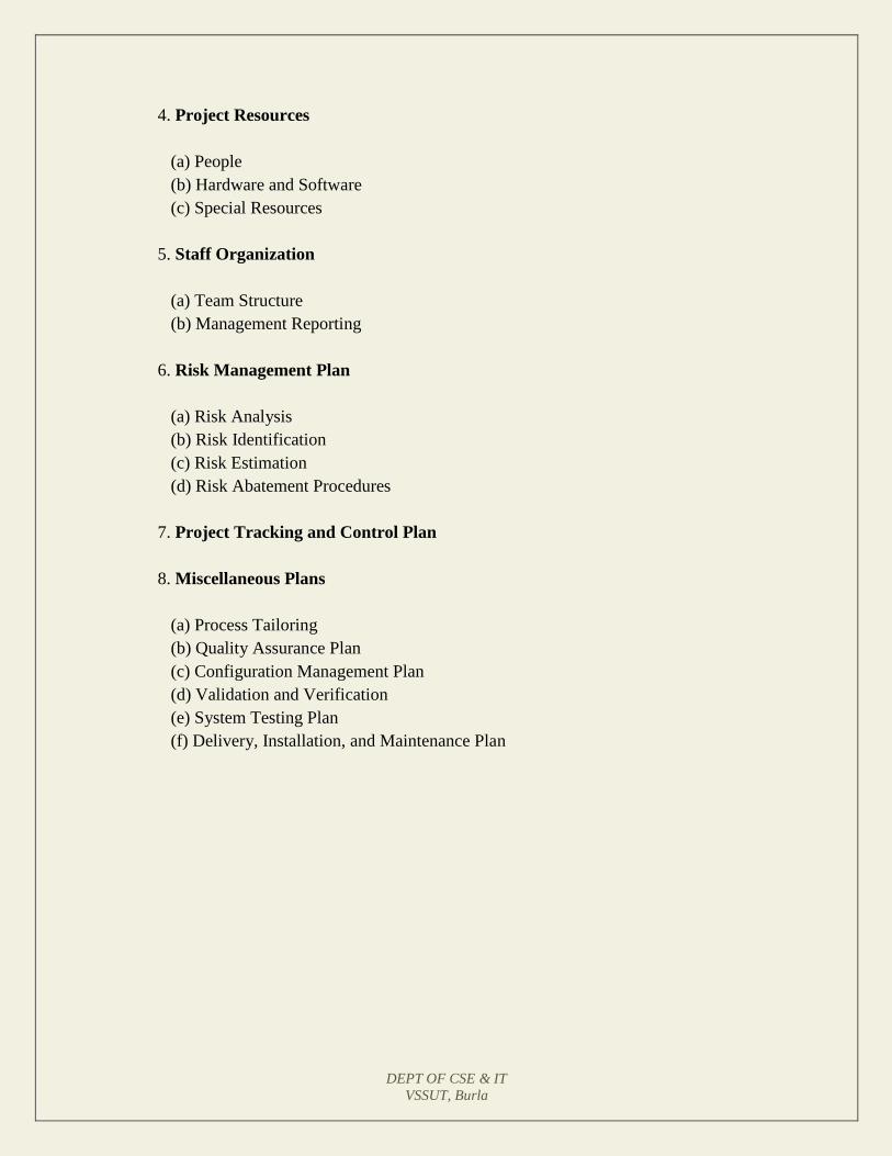
DEPT OF CSE & IT
VSSUT, Burla
4. Project Resources
(a) People
(b) Hardware and Software
(c) Special Resources
5. Staff Organization
(a) Team Structure
(b) Management Reporting
6. Risk Management Plan
(a) Risk Analysis
(b) Risk Identification
(c) Risk Estimation
(d) Risk Abatement Procedures
7. Project Tracking and Control Plan
8. Miscellaneous Plans
(a) Process Tailoring
(b) Quality Assurance Plan
(c) Configuration Management Plan
(d) Validation and Verification
(e) System Testing Plan
(f) Delivery, Installation, and Maintenance Plan
DEPT OF CSE & IT
VSSUT, Burla
LECTURE NOTE 31
METRICS FOR SOFTWARE PROJECT SIZE ESTIMATION
Accurate estimation of the problem size is fundamental to satisfactory estimation of effort, time
duration and cost of a software project. In order to be able to accurately estimate the project size,
some important metrics should be defined in terms of which the project size can be expressed.
The size of a problem is obviously not the number of bytes that the source code occupies. It is
neither the byte size of the executable code. The project size is a measure of the problem
complexity in terms of the effort and time required to develop the product.
Currently two metrics are popularly being used widely to estimate size: lines of code (LOC) and
function point (FP). The usage of each of these metrics in project size estimation has its own
advantages and disadvantages.
Lines of Code (LOC)
LOC is the simplest among all metrics available to estimate project size. This metric is very
popular because it is the simplest to use. Using this metric, the project size is estimated by
counting the number of source instructions in the developed program. Obviously, while counting
the number of source instructions, lines used for commenting the code and the header lines
should be ignored.
Determining the LOC count at the end of a project is a very simple job. However, accurate
estimation of the LOC count at the beginning of a project is very difficult. In order to estimate
the LOC count at the beginning of a project, project managers usually divide the problem into
modules, and each module into submodules and so on, until the sizes of the different leaf-level
modules can be approximately predicted. To be able to do this, past experience in developing
similar products is helpful. By using the estimation of the lowest level modules, project
managers arrive at the total size estimation.
Function point (FP)
Function point metric was proposed by Albrecht [1983]. This metric overcomes many of the
shortcomings of the LOC metric. Since its inception in late 1970s, function point metric has been
slowly gaining popularity. One of the important advantages of using the function point metric is
that it can be used to easily estimate the size of a software product directly from the problem
specification. This is in contrast to the LOC metric, where the size can be accurately determined
only after the product has fully been developed. The conceptual idea behind the function point
metric is that the size of a software product is directly dependent on the number of different
functions or features it supports. A software product supporting many features would certainly be
of larger size than a product with less number of features. Each function when invoked reads
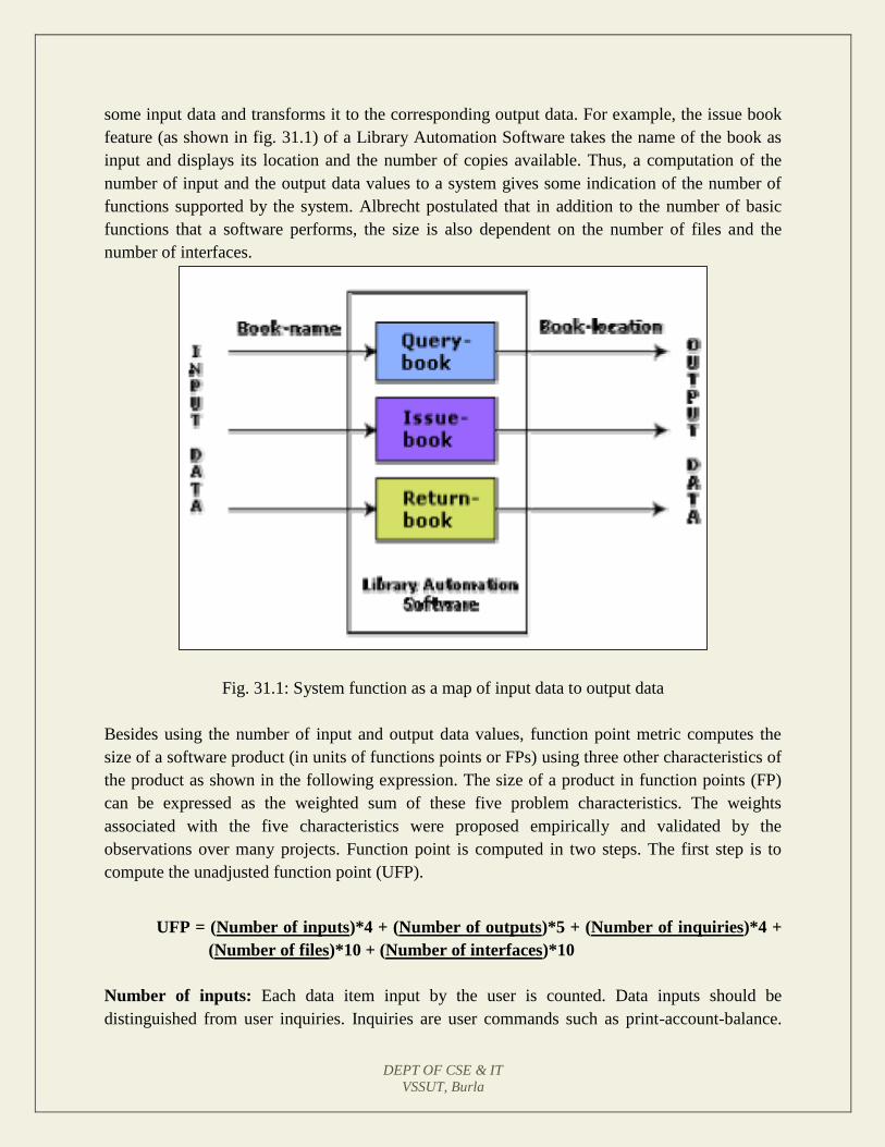
DEPT OF CSE & IT
VSSUT, Burla
some input data and transforms it to the corresponding output data. For example, the issue book
feature (as shown in fig. 31.1) of a Library Automation Software takes the name of the book as
input and displays its location and the number of copies available. Thus, a computation of the
number of input and the output data values to a system gives some indication of the number of
functions supported by the system. Albrecht postulated that in addition to the number of basic
functions that a software performs, the size is also dependent on the number of files and the
number of interfaces.
Fig. 31.1: System function as a map of input data to output data
Besides using the number of input and output data values, function point metric computes the
size of a software product (in units of functions points or FPs) using three other characteristics of
the product as shown in the following expression. The size of a product in function points (FP)
can be expressed as the weighted sum of these five problem characteristics. The weights
associated with the five characteristics were proposed empirically and validated by the
observations over many projects. Function point is computed in two steps. The first step is to
compute the unadjusted function point (UFP).
UFP = (Number of inputs)*4 + (Number of outputs)*5 + (Number of inquiries)*4 +
(Number of files)*10 + (Number of interfaces)*10
Number of inputs: Each data item input by the user is counted. Data inputs should be
distinguished from user inquiries. Inquiries are user commands such as print-account-balance.
DEPT OF CSE & IT
VSSUT, Burla
Inquiries are counted separately. It must be noted that individual data items input by the user are
not considered in the calculation of the number of inputs, but a group of related inputs are
considered as a single input. For example, while entering the data concerning an employee to an
employee pay roll software; the data items name, age, sex, address, phone number, etc. are
together considered as a single input. All these data items can be considered to be related, since
they pertain to a single employee.
Number of outputs: The outputs considered refer to reports printed, screen outputs, error
messages produced, etc. While outputting the number of outputs the individual data items within
a report are not considered, but a set of related data items is counted as one input.
Number of inquiries: Number of inquiries is the number of distinct interactive queries which
can be made by the users. These inquiries are the user commands which require specific action
by the system.
Number of files: Each logical file is counted. A logical file means groups of logically related
data. Thus, logical files can be data structures or physical files.
Number of interfaces: Here the interfaces considered are the interfaces used to exchange
information with other systems. Examples of such interfaces are data files on tapes, disks,
communication links with other systems etc.
Once the unadjusted function point (UFP) is computed, the technical complexity factor (TCF) is
computed next. TCF refines the UFP measure by considering fourteen other factors such as high
transaction rates, throughput, and response time requirements, etc. Each of these 14 factors is
assigned from 0 (not present or no influence) to 6 (strong influence). The resulting numbers are
summed, yielding the total degree of influence (DI). Now, TCF is computed as (0.65+0.01*DI).
As DI can vary from 0 to 70, TCF can vary from 0.65 to 1.35. Finally, FP=UFP*TCF.
Shortcomings of function point (FP) metric
LOC as a measure of problem size has several shortcomings:
LOC gives a numerical value of problem size that can vary widely with individual coding
style – different programmers lay out their code in different ways. For example, one
programmer might write several source instructions on a single line whereas another
might split a single instruction across several lines. Of course, this problem can be easily
overcome by counting the language tokens in the program rather than the lines of code.
However, a more intricate problem arises because the length of a program depends on the
choice of instructions used in writing the program. Therefore, even for the same problem,
different programmers might come up with programs having different LOC counts. This
situation does not improve even if language tokens are counted instead of lines of code.
DEPT OF CSE & IT
VSSUT, Burla
A good problem size measure should consider the overall complexity of the problem and
the effort needed to solve it. That is, it should consider the local effort needed to specify,
design, code, test, etc. and not just the coding effort. LOC, however, focuses on the
coding activity alone; it merely computes the number of source lines in the final program.
We have already seen that coding is only a small part of the overall software
development activities. It is also wrong to argue that the overall product development
effort is proportional to the effort required in writing the program code. This is because
even though the design might be very complex, the code might be straightforward and
vice versa. In such cases, code size is a grossly improper indicator of the problem size.
LOC measure correlates poorly with the quality and efficiency of the code. Larger code
size does not necessarily imply better quality or higher efficiency. Some programmers
produce lengthy and complicated code as they do not make effective use of the available
instruction set. In fact, it is very likely that a poor and sloppily written piece of code
might have larger number of source instructions than a piece that is neat and efficient.
LOC metric penalizes use of higher-level programming languages, code reuse, etc. The
paradox is that if a programmer consciously uses several library routines, then the LOC
count will be lower. This would show up as smaller program size. Thus, if managers use
the LOC count as a measure of the effort put in the different engineers (that is,
productivity), they would be discouraging code reuse by engineers.
LOC metric measures the lexical complexity of a program and does not address the more
important but subtle issues of logical or structural complexities. Between two programs
with equal LOC count, a program having complex logic would require much more effort
to develop than a program with very simple logic. To realize why this is so, consider the
effort required to develop a program having multiple nested loop and decision constructs
with another program having only sequential control flow.
It is very difficult to accurately estimate LOC in the final product from the problem
specification. The LOC count can be accurately computed only after the code has been
fully developed. Therefore, the LOC metric is little use to the project managers during
project planning, since project planning is carried out even before any development
activity has started. This possibly is the biggest shortcoming of the LOC metric from the
project manager’s perspective.
Feature Point Metric
A major shortcoming of the function point measure is that it does not take into account the
algorithmic complexity of a software. That is, the function point metric implicitly assumes that
the effort required to design and develop any two functionalities of the system is the same. But,
we know that this is normally not true, the effort required to develop any two functionalities may
vary widely. It only takes the number of functions that the system supports into consideration
DEPT OF CSE & IT
VSSUT, Burla
without distinguishing the difficulty level of developing the various functionalities. To overcome
this problem, an extension of the function point metric called feature point metric is proposed.
Feature point metric incorporates an extra parameter algorithm complexity. This parameter
ensures that the computed size using the feature point metric reflects the fact that the more is the
complexity of a function, the greater is the effort required to develop it and therefore its size
should be larger compared to simpler functions.
Project Estimation Techniques
Estimation of various project parameters is a basic project planning activity. The important
project parameters that are estimated include: project size, effort required to develop the
software, project duration, and cost. These estimates not only help in quoting the project cost to
the customer, but are also useful in resource planning and scheduling. There are three broad
categories of estimation techniques:
• Empirical estimation techniques
• Heuristic techniques
• Analytical estimation techniques
Empirical Estimation Techniques
Empirical estimation techniques are based on making an educated guess of the project
parameters. While using this technique, prior experience with development of similar
products is helpful. Although empirical estimation techniques are based on common
sense, different activities involved in estimation have been formalized over the years.
Two popular empirical estimation techniques are: Expert judgment technique and
Delphi cost estimation.
Expert Judgment Technique
Expert judgment is one of the most widely used estimation techniques. In this approach,
an expert makes an educated guess of the problem size after analyzing the problem
thoroughly. Usually, the expert estimates the cost of the different components (i.e.
modules or subsystems) of the system and then combines them to arrive at the overall
estimate. However, this technique is subject to human errors and individual bias. Also, it
is possible that the expert may overlook some factors inadvertently. Further, an expert
making an estimate may not have experience and knowledge of all aspects of a project.
For example, he may be conversant with the database and user interface parts but may not
be very knowledgeable about the computer communication part.
A more refined form of expert judgment is the estimation made by group of experts.
Estimation by a group of experts minimizes factors such as individual oversight, lack of
familiarity with a particular aspect of a project, personal bias, and the desire to win
contract through overly optimistic estimates. However, the estimate made by a group of
DEPT OF CSE & IT
VSSUT, Burla
experts may still exhibit bias on issues where the entire group of experts may be biased
due to reasons such as political considerations. Also, the decision made by the group may
be dominated by overly assertive members.
Delphi Cost Estimation
Delphi cost estimation approach tries to overcome some of the shortcomings of the expert
judgment approach. Delphi estimation is carried out by a team comprising of a group of
experts and a coordinator. In this approach, the coordinator provides each estimator with
a copy of the software requirements specification (SRS) document and a form for
recording his cost estimate. Estimators complete their individual estimates anonymously
and submit to the coordinator. In their estimates, the estimators mention any unusual
characteristic of the product which has influenced his estimation. The coordinator
prepares and distributes the summary of the responses of all the estimators, and includes
any unusual rationale noted by any of the estimators. Based on this summary, the
estimators re-estimate. This process is iterated for several rounds. However, no
discussion among the estimators is allowed during the entire estimation process. The idea
behind this is that if any discussion is allowed among the estimators, then many
estimators may easily get influenced by the rationale of an estimator who may be more
experienced or senior. After the completion of several iterations of estimations, the
coordinator takes the responsibility of compiling the results and preparing the final
estimate.
DEPT OF CSE & IT
VSSUT, Burla
LECTURE NOTE 32
HEURISTIC TECHNIQUES
Heuristic techniques assume that the relationships among the different project parameters can be
modeled using suitable mathematical expressions. Once the basic (independent) parameters are
known, the other (dependent) parameters can be easily determined by substituting the value of
the basic parameters in the mathematical expression. Different heuristic estimation models can
be divided into the following two classes: single variable model and the multi variable model.
Single variable estimation models provide a means to estimate the desired characteristics of a
problem, using some previously estimated basic (independent) characteristic of the software
product such as its size. A single variable estimation model takes the following form:
Estimated Parameter = c1
* ed
1
In the above expression, e is the characteristic of the software which has already been estimated
(independent variable). Estimated Parameter is the dependent parameter to be estimated. The
dependent parameter to be estimated could be effort, project duration, staff size, etc. c1
and d1
are
constants. The values of the constants c1
and d1
are usually determined using data collected from
past projects (historical data). The basic COCOMO model is an example of single variable cost
estimation model.
A multivariable cost estimation model takes the following form:
Estimated Resource = c1*e
1
d
1 + c
2*e
2
d
2 + ...
Where e1, e
2, … are the basic (independent) characteristics of the software already estimated, and
c1, c
2, d
1, d
2, … are constants. Multivariable estimation models are expected to give more
accurate estimates compared to the single variable models, since a project parameter is typically
influenced by several independent parameters. The independent parameters influence the
dependent parameter to different extents. This is modeled by the constants c1, c
2, d
1, d
2, … .
Values of these constants are usually determined from historical data. The intermediate
COCOMO model can be considered to be an example of a multivariable estimation model.
Analytical Estimation Techniques
Analytical estimation techniques derive the required results starting with basic assumptions
regarding the project. Thus, unlike empirical and heuristic techniques, analytical techniques do
have scientific basis. Halstead’s software science is an example of an analytical technique.
Halstead’s software science can be used to derive some interesting results starting with a few
DEPT OF CSE & IT
VSSUT, Burla
simple assumptions. Halstead’s software science is especially useful for estimating software
maintenance efforts. In fact, it outperforms both empirical and heuristic techniques when used
for predicting software maintenance efforts.
Halstead’s Software Science – An Analytical Technique
Halstead’s software science is an analytical technique to measure size, development effort, and
development cost of software products. Halstead used a few primitive program parameters to
develop the expressions for overall program length, potential minimum value, actual volume,
effort, and development time.
For a given program, let:
η1
be the number of unique operators used in the program,
η2
be the number of unique operands used in the program,
N1
be the total number of operators used in the program,
N2
be the total number of operands used in the program.
Length and Vocabulary
The length of a program as defined by Halstead, quantifies total usage of all operators and
operands in the program. Thus, length N = N1
+N2. Halstead’s definition of the length of the
program as the total number of operators and operands roughly agrees with the intuitive notation
of the program length as the total number of tokens used in the program.
The program vocabulary is the number of unique operators and operands used in the program.
Thus, program vocabulary η = η1
+ η2.
Program Volume
The length of a program (i.e. the total number of operators and operands used in the code)
depends on the choice of the operators and operands used. In other words, for the same
programming problem, the length would depend on the programming style. This type of
dependency would produce different measures of length for essentially the same problem when
different programming languages are used. Thus, while expressing program size, the
programming language used must be taken into consideration:
V = Nlog2η
Here the program volume V is the minimum number of bits needed to encode the program. In
fact, to represent η different identifiers uniquely, at least log2η bits (where η is the program
vocabulary) will be needed. In this scheme, Nlog2η bits will be needed to store a program of
length N. Therefore, the volume V represents the size of the program by approximately
compensating for the effect of the programming language used.

DEPT OF CSE & IT
VSSUT, Burla
Potential Minimum Volume
The potential minimum volume V* is defined as the volume of most succinct program in which a
problem can be coded. The minimum volume is obtained when the program can be expressed
using a single source code instruction. say a function call like foo( ) ;. In other words, the volume
is bound from below due to the fact that a program would have at least two operators and no less
than the requisite number of operands.
Thus, if an algorithm operates on input and output data d1, d
2, … d
n, the most succinct program
would be f(d1, d
2, … d
n); for which η
1 = 2, η
2 = n. Therefore, V* = (2 + η
2)log
2(2 + η
2).
The program level L is given by L = V*/V. The concept of program level L is introduced in an
attempt to measure the level of abstraction provided by the programming language. Using this
definition, languages can be ranked into levels that also appear intuitively correct.
The above result implies that the higher the level of a language, the less effort it takes to develop
a program using that language. This result agrees with the intuitive notion that it takes more
effort to develop a program in assembly language than to develop a program in a high-level
language to solve a problem.
Effort and Time
The effort required to develop a program can be obtained by dividing the program volume with
the level of the programming language used to develop the code. Thus, effort E = V/L, where E
is the number of mental discriminations required to implement the program and also the effort
required to read and understand the program. Thus, the programming effort E = V²/V* (since L =
V*/V) varies as the square of the volume. Experience shows that E is well correlated to the effort
needed for maintenance of an existing program.
The programmer’s time T = E/S, where S the speed of mental discriminations. The value of S
has been empirically developed from psychological reasoning, and its recommended value for
programming applications is 18.
Length Estimation
Even though the length of a program can be found by calculating the total number of operators
and operands in a program, Halstead suggests a way to determine the length of a program using
the number of unique operators and operands used in the program. Using this method, the
program parameters such as length, volume, cost, effort, etc. can be determined even before the
start of any programming activity. His method is summarized below.

DEPT OF CSE & IT
VSSUT, Burla
Halstead assumed that it is quite unlikely that a program has several identical parts – in formal
language terminology identical substrings – of length greater than η (η being the program
vocabulary). In fact, once a piece of code occurs identically at several places, it is made into a
procedure or a function. Thus, it can be assumed that any program of length N consists of N/ η
unique strings of length η. Now, it is standard combinatorial result that for any given alphabet of
size K, there are exactly Kr
different strings of length r.
Thus.
N/η ≤ ηη
Or, N ≤ ηη+1
Since operators and operands usually alternate in a program, the upper bound can be further
refined into N ≤ η η1
η1
η2
η2
. Also, N must include not only the ordered set of n elements, but it
should also include all possible subsets of that ordered sets, i.e. the power set of N strings (This
particular reasoning of Halstead is not very convincing!!!).
Therefore,
2N
= η η1
η1
η2
η2
Or, taking logarithm on both sides,
N = log2η +log
2(η
1
η1
η2
η2
)
So we get,
N = log 2(η
1
η1
η2
η2
)
(approximately, by ignoring log2η)
Or,
N = log2η
1
η1
+ log2η
2
η2
= η1log
2η
1 + η
2log
2η
2
Experimental evidence gathered from the analysis of larger number of programs suggests that the
computed and actual lengths match very closely. However, the results may be inaccurate when
small programs when considered individually.
In conclusion, Halstead’s theory tries to provide a formal definition and quantification of such
qualitative attributes as program complexity, ease of understanding, and the level of abstraction
based on some low-level parameters such as the number of operands, and operators appearing in
DEPT OF CSE & IT
VSSUT, Burla
the program. Halstead’s software science provides gross estimation of properties of a large
collection of software, but extends to individual cases rather inaccurately.
Example:
Let us consider the following C program:
main( )
{
int a, b, c, avg;
scanf(“%d %d %d”, &a, &b, &c);
avg = (a+b+c)/3;
printf(“avg = %d”, avg);
}
The unique operators are:
main,(),{},int,scanf,&,“,”,“;”,=,+,/, printf
The unique operands are:
a, b, c, &a, &b, &c, a+b+c, avg, 3,
“%d %d %d”, “avg = %d”
Therefore,
η1
= 12, η2
= 11
Estimated Length = (12*log12 + 11*log11)
= (12*3.58 + 11*3.45)
= (43+38) = 81
Volume = Length*log(23)
= 81*4.52
= 366
DEPT OF CSE & IT
VSSUT, Burla
LECTURE NOTE 33
COCOMO MODEL
Organic, Semidetached and Embedded software projects
Boehm postulated that any software development project can be classified into one of the
following three categories based on the development complexity: organic, semidetached, and
embedded. In order to classify a product into the identified categories, Boehm not only
considered the characteristics of the product but also those of the development team and
development environment. Roughly speaking, these three product classes correspond to
application, utility and system programs, respectively. Normally, data processing programs are
considered to be application programs. Compilers, linkers, etc., are utility programs. Operating
systems and real-time system programs, etc. are system programs. System programs interact
directly with the hardware and typically involve meeting timing constraints and concurrent
processing.
Boehm’s [1981] definition of organic, semidetached, and embedded systems are elaborated
below.
Organic: A development project can be considered of organic type, if the project deals with
developing a well understood application program, the size of the development team is
reasonably small, and the team members are experienced in developing similar types of projects.
Semidetached: A development project can be considered of semidetached type, if the
development consists of a mixture of experienced and inexperienced staff. Team members may
have limited experience on related systems but may be unfamiliar with some aspects of the
system being developed.
Embedded: A development project is considered to be of embedded type, if the software being
developed is strongly coupled to complex hardware, or if the stringent regulations on the
operational procedures exist.
COCOMO
COCOMO (Constructive Cost Estimation Model) was proposed by Boehm [1981]. According to
Boehm, software cost estimation should be done through three stages: Basic COCOMO,
Intermediate COCOMO, and Complete COCOMO.
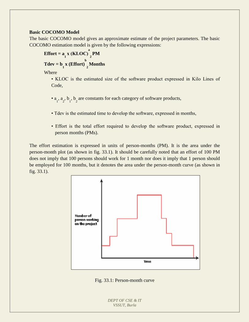
DEPT OF CSE & IT
VSSUT, Burla
Basic COCOMO Model
The basic COCOMO model gives an approximate estimate of the project parameters. The basic
COCOMO estimation model is given by the following expressions:
Effort = a1
х (KLOC)a
2 PM
Tdev = b1 x (Effort)
b
2 Months
Where
• KLOC is the estimated size of the software product expressed in Kilo Lines of
Code,
• a1, a
2, b
1, b
2 are constants for each category of software products,
• Tdev is the estimated time to develop the software, expressed in months,
• Effort is the total effort required to develop the software product, expressed in
person months (PMs).
The effort estimation is expressed in units of person-months (PM). It is the area under the
person-month plot (as shown in fig. 33.1). It should be carefully noted that an effort of 100 PM
does not imply that 100 persons should work for 1 month nor does it imply that 1 person should
be employed for 100 months, but it denotes the area under the person-month curve (as shown in
fig. 33.1).
Fig. 33.1: Person-month curve
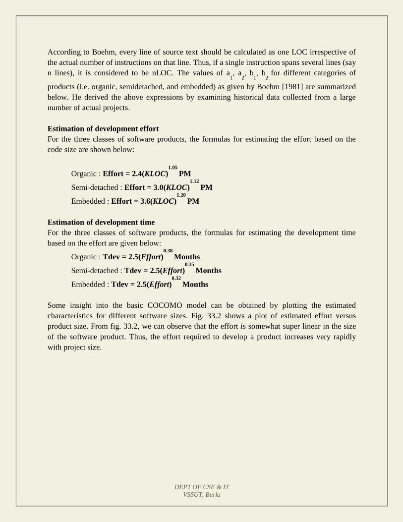
DEPT OF CSE & IT
VSSUT, Burla
According to Boehm, every line of source text should be calculated as one LOC irrespective of
the actual number of instructions on that line. Thus, if a single instruction spans several lines (say
n lines), it is considered to be nLOC. The values of a1, a
2, b
1, b
2 for different categories of
products (i.e. organic, semidetached, and embedded) as given by Boehm [1981] are summarized
below. He derived the above expressions by examining historical data collected from a large
number of actual projects.
Estimation of development effort
For the three classes of software products, the formulas for estimating the effort based on the
code size are shown below:
Organic : Effort = 2.4(KLOC)1.05
PM
Semi-detached : Effort = 3.0(KLOC)1.12
PM
Embedded : Effort = 3.6(KLOC)1.20
PM
Estimation of development time
For the three classes of software products, the formulas for estimating the development time
based on the effort are given below:
Organic : Tdev = 2.5(Effort)0.38
Months
Semi-detached : Tdev = 2.5(Effort)0.35
Months
Embedded : Tdev = 2.5(Effort)0.32
Months
Some insight into the basic COCOMO model can be obtained by plotting the estimated
characteristics for different software sizes. Fig. 33.2 shows a plot of estimated effort versus
product size. From fig. 33.2, we can observe that the effort is somewhat super linear in the size
of the software product. Thus, the effort required to develop a product increases very rapidly
with project size.
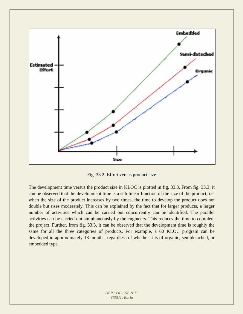
DEPT OF CSE & IT
VSSUT, Burla
Fig. 33.2: Effort versus product size
The development time versus the product size in KLOC is plotted in fig. 33.3. From fig. 33.3, it
can be observed that the development time is a sub linear function of the size of the product, i.e.
when the size of the product increases by two times, the time to develop the product does not
double but rises moderately. This can be explained by the fact that for larger products, a larger
number of activities which can be carried out concurrently can be identified. The parallel
activities can be carried out simultaneously by the engineers. This reduces the time to complete
the project. Further, from fig. 33.3, it can be observed that the development time is roughly the
same for all the three categories of products. For example, a 60 KLOC program can be
developed in approximately 18 months, regardless of whether it is of organic, semidetached, or
embedded type.

DEPT OF CSE & IT
VSSUT, Burla
Fig. 33.3: Development time versus size
From the effort estimation, the project cost can be obtained by multiplying the required effort by
the manpower cost per month. But, implicit in this project cost computation is the assumption
that the entire project cost is incurred on account of the manpower cost alone. In addition to
manpower cost, a project would incur costs due to hardware and software required for the project
and the company overheads for administration, office space, etc.
It is important to note that the effort and the duration estimations obtained using the COCOMO
model are called as nominal effort estimate and nominal duration estimate. The term nominal
implies that if anyone tries to complete the project in a time shorter than the estimated duration,
then the cost will increase drastically. But, if anyone completes the project over a longer period
of time than the estimated, then there is almost no decrease in the estimated cost value.
DEPT OF CSE & IT
VSSUT, Burla
Example:
Assume that the size of an org organic type software product has been estimated to be 32,000
lines of source code. Assume that the average salary of software engineers be Rs. 15,000/- per
month. Determine the effort required to develop the software product and the nominal
development time.
From the basic COCOMO estimation formula for organic software:
Effort = 2.4 х (32)1.05
= 91 PM
Nominal development time = 2.5 х (91)0.38
= 14 months
Cost required to develop the product = 14 х 15,000
= Rs. 210,000/-
DEPT OF CSE & IT
VSSUT, Burla
LECTURE NOTE 34
INTERMEDIATE COCOMO MODEL
The basic COCOMO model assumes that effort and development time are functions of the
product size alone. However, a host of other project parameters besides the product size affect
the effort required to develop the product as well as the development time. Therefore, in order to
obtain an accurate estimation of the effort and project duration, the effect of all relevant
parameters must be taken into account. The intermediate COCOMO model recognizes this fact
and refines the initial estimate obtained using the basic COCOMO expressions by using a set of
15 cost drivers (multipliers) based on various attributes of software development. For example, if
modern programming practices are used, the initial estimates are scaled downward by
multiplication with a cost driver having a value less than 1. If there are stringent reliability
requirements on the software product, this initial estimate is scaled upward. Boehm requires the
project manager to rate these 15 different parameters for a particular project on a scale of one to
three. Then, depending on these ratings, he suggests appropriate cost driver values which should
be multiplied with the initial estimate obtained using the basic COCOMO. In general, the cost
drivers can be classified as being attributes of the following items:
Product: The characteristics of the product that are considered include the inherent complexity
of the product, reliability requirements of the product, etc.
Computer: Characteristics of the computer that are considered include the execution speed
required, storage space required etc.
Personnel: The attributes of development personnel that are considered include the experience
level of personnel, programming capability, analysis capability, etc.
Development Environment: Development environment attributes capture the development
facilities available to the developers. An important parameter that is considered is the
sophistication of the automation (CASE) tools used for software development.
Complete COCOMO model
A major shortcoming of both the basic and intermediate COCOMO models is that they consider
a software product as a single homogeneous entity. However, most large systems are made up
several smaller sub-systems. These sub-systems may have widely different characteristics. For
example, some sub-systems may be considered as organic type, some semidetached, and some
embedded. Not only that the inherent development complexity of the subsystems may be
different, but also for some subsystems the reliability requirements may be high, for some the
DEPT OF CSE & IT
VSSUT, Burla
development team might have no previous experience of similar development, and so on. The
complete COCOMO model considers these differences in characteristics of the subsystems and
estimates the effort and development time as the sum of the estimates for the individual
subsystems. The cost of each subsystem is estimated separately. This approach reduces the
margin of error in the final estimate.
The following development project can be considered as an example application of the complete
COCOMO model. A distributed Management Information System (MIS) product for an
organization having offices at several places across the country can have the following sub-
components:
• Database part
• Graphical User Interface (GUI) part
• Communication part
Of these, the communication part can be considered as embedded software. The database part
could be semi-detached software, and the GUI part organic software. The costs for these three
components can be estimated separately, and summed up to give the overall cost of the system.

DEPT OF CSE & IT
VSSUT, Burla
LECTURE NOTE 35
STAFFING LEVEL ESTIMATION
Once the effort required to develop a software has been determined, it is necessary to determine
the staffing requirement for the project. Putnam first studied the problem of what should be a
proper staffing pattern for software projects. He extended the work of Norden who had earlier
investigated the staffing pattern of research and development (R&D) type of projects. In order to
appreciate the staffing pattern of software projects, Norden’s and Putnam’s results must be
understood.
Norden’s Work
Norden studied the staffing patterns of several R & D projects. He found that the staffing pattern
can be approximated by the Rayleigh distribution curve (as shown in fig. 35.1). Norden
represented the Rayleigh curve by the following equation:
E = K/t²d
* t * e-t² / 2 t²
d
Where E is the effort required at time t. E is an indication of the number of engineers (or the
staffing level) at any particular time during the duration of the project, K is the area under the
curve, and td
is the time at which the curve attains its maximum value. It must be remembered
that the results of Norden are applicable to general R & D projects and were not meant to model
the staffing pattern of software development projects.
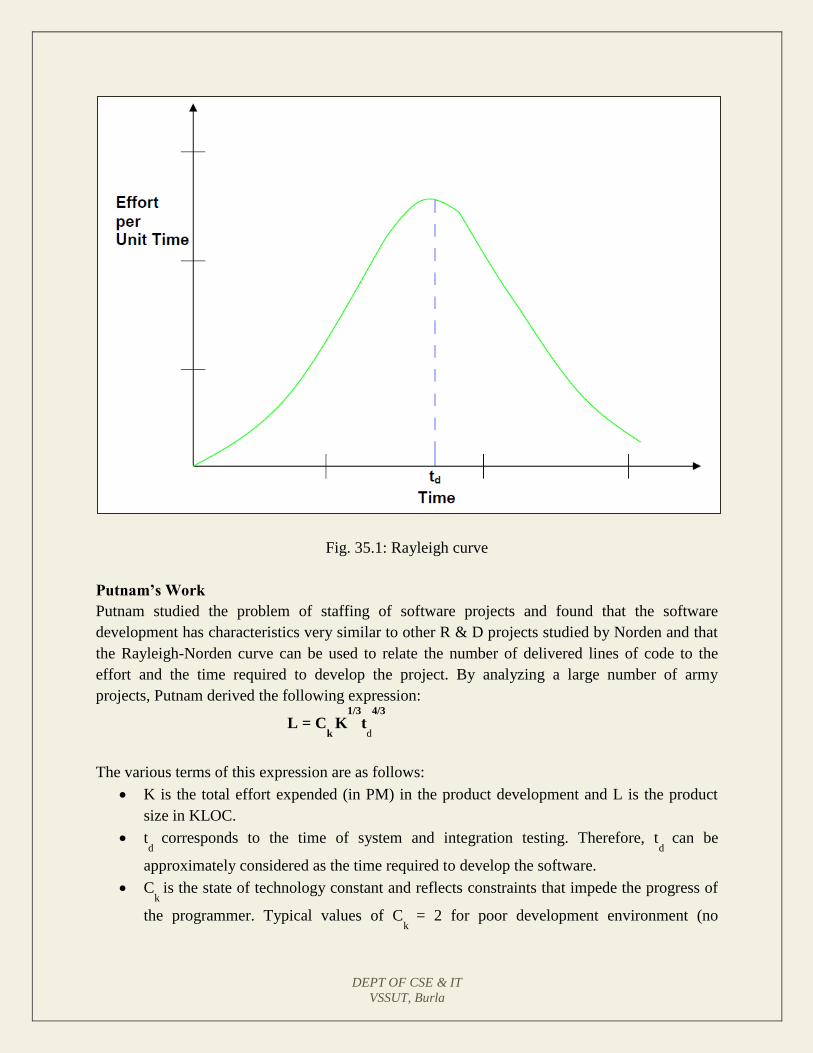
DEPT OF CSE & IT
VSSUT, Burla
Fig. 35.1: Rayleigh curve
Putnam’s Work
Putnam studied the problem of staffing of software projects and found that the software
development has characteristics very similar to other R & D projects studied by Norden and that
the Rayleigh-Norden curve can be used to relate the number of delivered lines of code to the
effort and the time required to develop the project. By analyzing a large number of army
projects, Putnam derived the following expression:
L = Ck
K1/3
td
4/3
The various terms of this expression are as follows:
K is the total effort expended (in PM) in the product development and L is the product
size in KLOC.
td
corresponds to the time of system and integration testing. Therefore, td
can be
approximately considered as the time required to develop the software.
Ck
is the state of technology constant and reflects constraints that impede the progress of
the programmer. Typical values of Ck
= 2 for poor development environment (no
DEPT OF CSE & IT
VSSUT, Burla
methodology, poor documentation, and review, etc.), Ck
= 8 for good software
development environment (software engineering principles are adhered to), Ck
= 11 for an
excellent environment (in addition to following software engineering principles,
automated tools and techniques are used). The exact value of Ck
for a specific project can
be computed from the historical data of the organization developing it.
Putnam suggested that optimal staff build-up on a project should follow the Rayleigh curve.
Only a small number of engineers are needed at the beginning of a project to carry out planning
and specification tasks. As the project progresses and more detailed work is required, the number
of engineers reaches a peak. After implementation and unit testing, the number of project staff
falls.
However, the staff build-up should not be carried out in large installments. The team size should
either be increased or decreased slowly whenever required to match the Rayleigh-Norden curve.
Experience shows that a very rapid build up of project staff any time during the project
development correlates with schedule slippage.
It should be clear that a constant level of manpower throughout the project duration would lead
to wastage of effort and increase the time and effort required to develop the product. If a constant
number of engineers are used over all the phases of a project, some phases would be overstaffed
and the other phases would be understaffed causing inefficient use of manpower, leading to
schedule slippage and increase in cost.
Effect of schedule change on cost
By analyzing a large number of army projects, Putnam derived the following expression:
L = Ck
K1/3
td
4/3
Where, K is the total effort expended (in PM) in the product development and L is the product
size in KLOC, td
corresponds to the time of system and integration testing and Ck
is the state of
technology constant and reflects constraints that impede the progress of the programmer
Now by using the above expression it is obtained that,
K = L3/C
k
3
td
4
Or,
K = C/td
4
For the same product size, C = L3 / Ck
3
is a constant.

DEPT OF CSE & IT
VSSUT, Burla
or, K1/K2 = td24/ td1
4
or, K ∝ 1/td
4
or, cost ∝ 1/td
(as project development effort is equally proportional to project development cost)
From the above expression, it can be easily observed that when the schedule of a project is
compressed, the required development effort as well as project development cost increases in
proportion to the fourth power of the degree of compression. It means that a relatively small
compression in delivery schedule can result in substantial penalty of human effort as well as
development cost. For example, if the estimated development time is 1 year, then in order to
develop the product in 6 months, the total effort required to develop the product (and hence the
project cost) increases 16 times.
DEPT OF CSE & IT
VSSUT, Burla
LECTURE NOTE 36
PROJECT SCHEDULING
Project-task scheduling is an important project planning activity. It involves deciding which
tasks would be taken up when. In order to schedule the project activities, a software project
manager needs to do the following:
1. Identify all the tasks needed to complete the project.
2. Break down large tasks into small activities.
3. Determine the dependency among different activities.
4. Establish the most likely estimates for the time durations necessary to complete the
activities.
5. Allocate resources to activities.
6. Plan the starting and ending dates for various activities.
7. Determine the critical path. A critical path is the chain of activities that determines the
duration of the project.
The first step in scheduling a software project involves identifying all the tasks necessary to
complete the project. A good knowledge of the intricacies of the project and the development
process helps the managers to effectively identify the important tasks of the project. Next, the
large tasks are broken down into a logical set of small activities which would be assigned to
different engineers. The work breakdown structure formalism helps the manager to breakdown
the tasks systematically after the project manager has broken down the tasks and created the
work breakdown structure, he has to find the dependency among the activities. Dependency
among the different activities determines the order in which the different activities would be
carried out. If an activity A requires the results of another activity B, then activity A must be
scheduled after activity B. In general, the task dependencies define a partial ordering among
tasks, i.e. each tasks may precede a subset of other tasks, but some tasks might not have any
precedence ordering defined between them (called concurrent task). The dependency among the
activities is represented in the form of an activity network.
Once the activity network representation has been worked out, resources are allocated to each
activity. Resource allocation is typically done using a Gantt chart. After resource allocation is
done, a PERT chart representation is developed. The PERT chart representation is suitable for
program monitoring and control. For task scheduling, the project manager needs to decompose
the project tasks into a set of activities. The time frame when each activity is to be performed is
to be determined. The end of each activity is called milestone. The project manager tracks the
progress of a project by monitoring the timely completion of the milestones. If he observes that
the milestones start getting delayed, then he has to carefully control the activities, so that the
overall deadline can still be met.
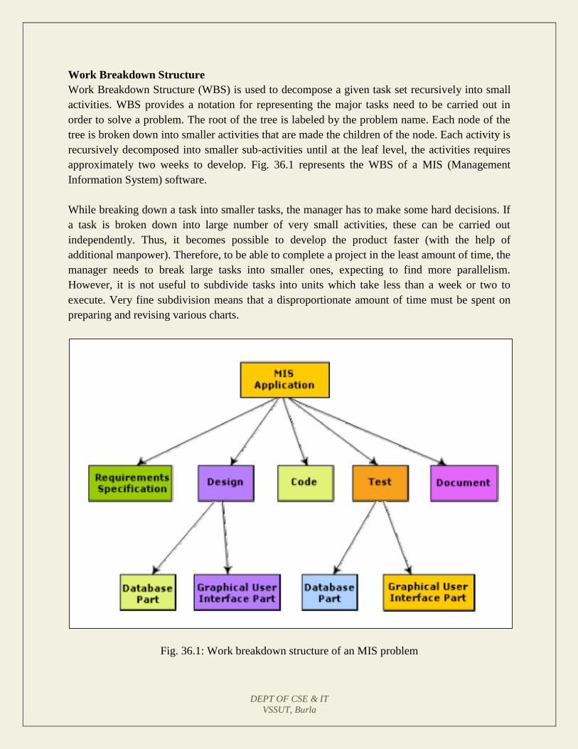
DEPT OF CSE & IT
VSSUT, Burla
Work Breakdown Structure
Work Breakdown Structure (WBS) is used to decompose a given task set recursively into small
activities. WBS provides a notation for representing the major tasks need to be carried out in
order to solve a problem. The root of the tree is labeled by the problem name. Each node of the
tree is broken down into smaller activities that are made the children of the node. Each activity is
recursively decomposed into smaller sub-activities until at the leaf level, the activities requires
approximately two weeks to develop. Fig. 36.1 represents the WBS of a MIS (Management
Information System) software.
While breaking down a task into smaller tasks, the manager has to make some hard decisions. If
a task is broken down into large number of very small activities, these can be carried out
independently. Thus, it becomes possible to develop the product faster (with the help of
additional manpower). Therefore, to be able to complete a project in the least amount of time, the
manager needs to break large tasks into smaller ones, expecting to find more parallelism.
However, it is not useful to subdivide tasks into units which take less than a week or two to
execute. Very fine subdivision means that a disproportionate amount of time must be spent on
preparing and revising various charts.
Fig. 36.1: Work breakdown structure of an MIS problem
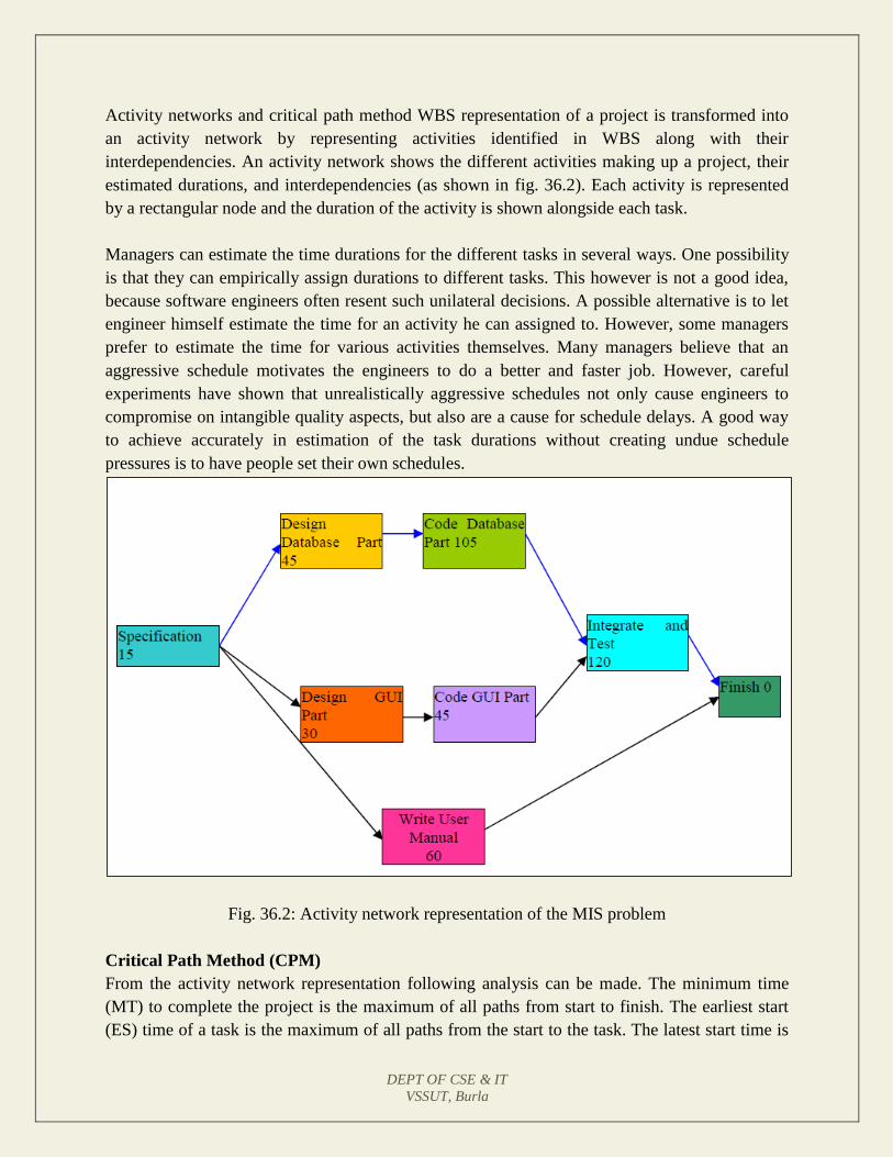
DEPT OF CSE & IT
VSSUT, Burla
Activity networks and critical path method WBS representation of a project is transformed into
an activity network by representing activities identified in WBS along with their
interdependencies. An activity network shows the different activities making up a project, their
estimated durations, and interdependencies (as shown in fig. 36.2). Each activity is represented
by a rectangular node and the duration of the activity is shown alongside each task.
Managers can estimate the time durations for the different tasks in several ways. One possibility
is that they can empirically assign durations to different tasks. This however is not a good idea,
because software engineers often resent such unilateral decisions. A possible alternative is to let
engineer himself estimate the time for an activity he can assigned to. However, some managers
prefer to estimate the time for various activities themselves. Many managers believe that an
aggressive schedule motivates the engineers to do a better and faster job. However, careful
experiments have shown that unrealistically aggressive schedules not only cause engineers to
compromise on intangible quality aspects, but also are a cause for schedule delays. A good way
to achieve accurately in estimation of the task durations without creating undue schedule
pressures is to have people set their own schedules.
Fig. 36.2: Activity network representation of the MIS problem
Critical Path Method (CPM)
From the activity network representation following analysis can be made. The minimum time
(MT) to complete the project is the maximum of all paths from start to finish. The earliest start
(ES) time of a task is the maximum of all paths from the start to the task. The latest start time is
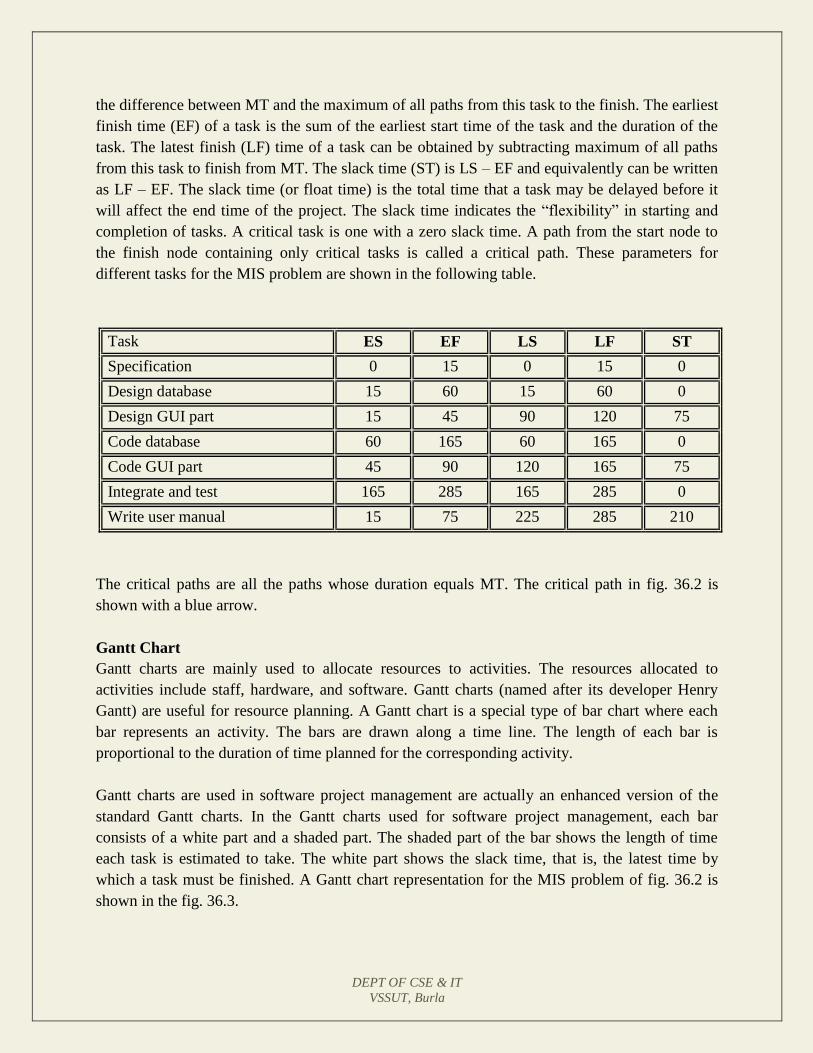
DEPT OF CSE & IT
VSSUT, Burla
the difference between MT and the maximum of all paths from this task to the finish. The earliest
finish time (EF) of a task is the sum of the earliest start time of the task and the duration of the
task. The latest finish (LF) time of a task can be obtained by subtracting maximum of all paths
from this task to finish from MT. The slack time (ST) is LS – EF and equivalently can be written
as LF – EF. The slack time (or float time) is the total time that a task may be delayed before it
will affect the end time of the project. The slack time indicates the “flexibility” in starting and
completion of tasks. A critical task is one with a zero slack time. A path from the start node to
the finish node containing only critical tasks is called a critical path. These parameters for
different tasks for the MIS problem are shown in the following table.
Task ES EF LS LF ST
Specification 0 15 0 15 0
Design database 15 60 15 60 0
Design GUI part 15 45 90 120 75
Code database 60 165 60 165 0
Code GUI part 45 90 120 165 75
Integrate and test 165 285 165 285 0
Write user manual 15 75 225 285 210
The critical paths are all the paths whose duration equals MT. The critical path in fig. 36.2 is
shown with a blue arrow.
Gantt Chart
Gantt charts are mainly used to allocate resources to activities. The resources allocated to
activities include staff, hardware, and software. Gantt charts (named after its developer Henry
Gantt) are useful for resource planning. A Gantt chart is a special type of bar chart where each
bar represents an activity. The bars are drawn along a time line. The length of each bar is
proportional to the duration of time planned for the corresponding activity.
Gantt charts are used in software project management are actually an enhanced version of the
standard Gantt charts. In the Gantt charts used for software project management, each bar
consists of a white part and a shaded part. The shaded part of the bar shows the length of time
each task is estimated to take. The white part shows the slack time, that is, the latest time by
which a task must be finished. A Gantt chart representation for the MIS problem of fig. 36.2 is
shown in the fig. 36.3.
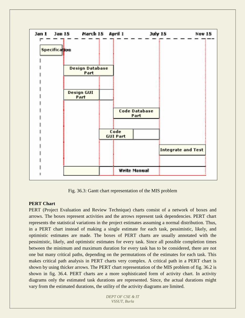
DEPT OF CSE & IT
VSSUT, Burla
Fig. 36.3: Gantt chart representation of the MIS problem
PERT Chart
PERT (Project Evaluation and Review Technique) charts consist of a network of boxes and
arrows. The boxes represent activities and the arrows represent task dependencies. PERT chart
represents the statistical variations in the project estimates assuming a normal distribution. Thus,
in a PERT chart instead of making a single estimate for each task, pessimistic, likely, and
optimistic estimates are made. The boxes of PERT charts are usually annotated with the
pessimistic, likely, and optimistic estimates for every task. Since all possible completion times
between the minimum and maximum duration for every task has to be considered, there are not
one but many critical paths, depending on the permutations of the estimates for each task. This
makes critical path analysis in PERT charts very complex. A critical path in a PERT chart is
shown by using thicker arrows. The PERT chart representation of the MIS problem of fig. 36.2 is
shown in fig. 36.4. PERT charts are a more sophisticated form of activity chart. In activity
diagrams only the estimated task durations are represented. Since, the actual durations might
vary from the estimated durations, the utility of the activity diagrams are limited.
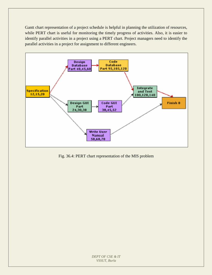
DEPT OF CSE & IT
VSSUT, Burla
Gantt chart representation of a project schedule is helpful in planning the utilization of resources,
while PERT chart is useful for monitoring the timely progress of activities. Also, it is easier to
identify parallel activities in a project using a PERT chart. Project managers need to identify the
parallel activities in a project for assignment to different engineers.
Fig. 36.4: PERT chart representation of the MIS problem
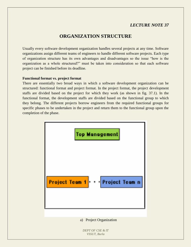
DEPT OF CSE & IT
VSSUT, Burla
LECTURE NOTE 37
ORGANIZATION STRUCTURE
Usually every software development organization handles several projects at any time. Software
organizations assign different teams of engineers to handle different software projects. Each type
of organization structure has its own advantages and disadvantages so the issue “how is the
organization as a whole structured?” must be taken into consideration so that each software
project can be finished before its deadline.
Functional format vs. project format
There are essentially two broad ways in which a software development organization can be
structured: functional format and project format. In the project format, the project development
staffs are divided based on the project for which they work (as shown in fig. 37.1). In the
functional format, the development staffs are divided based on the functional group to which
they belong. The different projects borrow engineers from the required functional groups for
specific phases to be undertaken in the project and return them to the functional group upon the
completion of the phase.
a) Project Organization
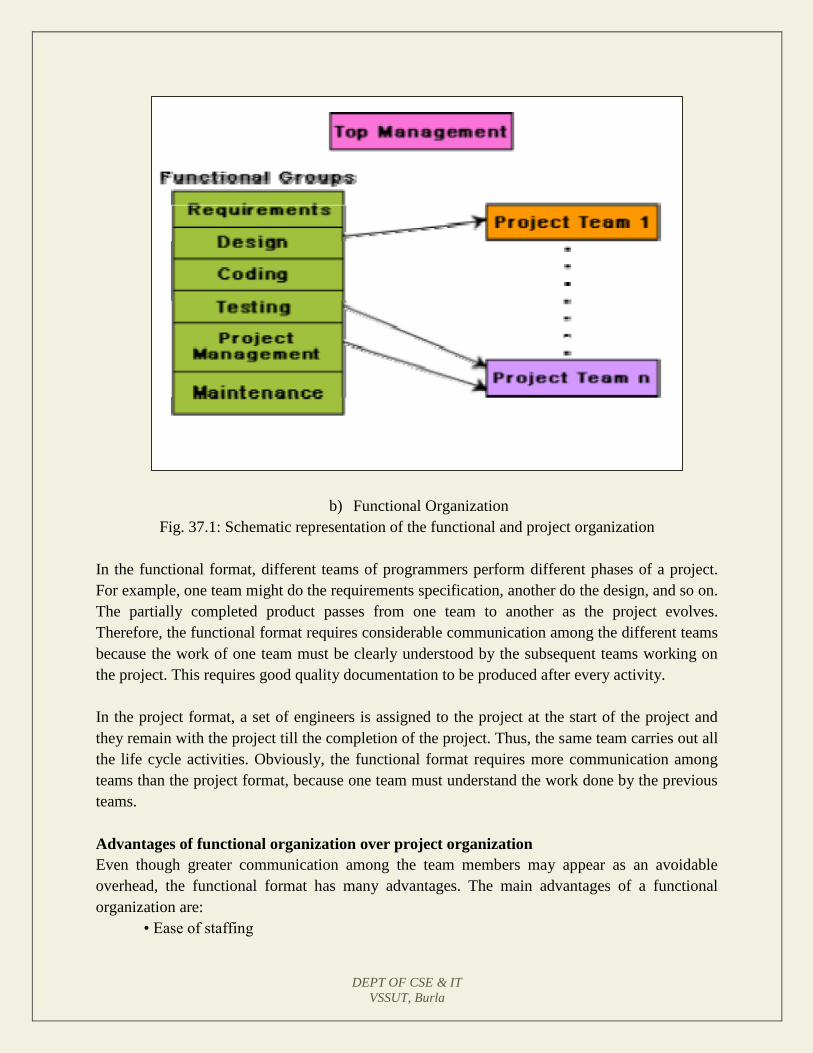
DEPT OF CSE & IT
VSSUT, Burla
b) Functional Organization
Fig. 37.1: Schematic representation of the functional and project organization
In the functional format, different teams of programmers perform different phases of a project.
For example, one team might do the requirements specification, another do the design, and so on.
The partially completed product passes from one team to another as the project evolves.
Therefore, the functional format requires considerable communication among the different teams
because the work of one team must be clearly understood by the subsequent teams working on
the project. This requires good quality documentation to be produced after every activity.
In the project format, a set of engineers is assigned to the project at the start of the project and
they remain with the project till the completion of the project. Thus, the same team carries out all
the life cycle activities. Obviously, the functional format requires more communication among
teams than the project format, because one team must understand the work done by the previous
teams.
Advantages of functional organization over project organization
Even though greater communication among the team members may appear as an avoidable
overhead, the functional format has many advantages. The main advantages of a functional
organization are:
• Ease of staffing
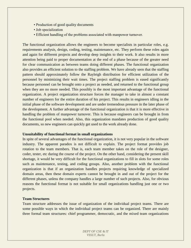
DEPT OF CSE & IT
VSSUT, Burla
• Production of good quality documents
• Job specialization
• Efficient handling of the problems associated with manpower turnover.
The functional organization allows the engineers to become specialists in particular roles, e.g.
requirements analysis, design, coding, testing, maintenance, etc. They perform these roles again
and again for different projects and develop deep insights to their work. It also results in more
attention being paid to proper documentation at the end of a phase because of the greater need
for clear communication as between teams doing different phases. The functional organization
also provides an efficient solution to the staffing problem. We have already seen that the staffing
pattern should approximately follow the Rayleigh distribution for efficient utilization of the
personnel by minimizing their wait times. The project staffing problem is eased significantly
because personnel can be brought onto a project as needed, and returned to the functional group
when they are no more needed. This possibly is the most important advantage of the functional
organization. A project organization structure forces the manager to take in almost a constant
number of engineers for the entire duration of his project. This results in engineers idling in the
initial phase of the software development and are under tremendous pressure in the later phase of
the development. A further advantage of the functional organization is that it is more effective in
handling the problem of manpower turnover. This is because engineers can be brought in from
the functional pool when needed. Also, this organization mandates production of good quality
documents, so new engineers can quickly get used to the work already done.
Unsuitability of functional format in small organizations
In spite of several advantages of the functional organization, it is not very popular in the software
industry. The apparent paradox is not difficult to explain. The project format provides job
rotation to the team members. That is, each team member takes on the role of the designer,
coder, tester, etc during the course of the project. On the other hand, considering the present skill
shortage, it would be very difficult for the functional organizations to fill in slots for some roles
such as maintenance, testing, and coding groups. Also, another problem with the functional
organization is that if an organization handles projects requiring knowledge of specialized
domain areas, then these domain experts cannot be brought in and out of the project for the
different phases, unless the company handles a large number of such projects. Also, for obvious
reasons the functional format is not suitable for small organizations handling just one or two
projects.
Team Structures
Team structure addresses the issue of organization of the individual project teams. There are
some possible ways in which the individual project teams can be organized. There are mainly
three formal team structures: chief programmer, democratic, and the mixed team organizations
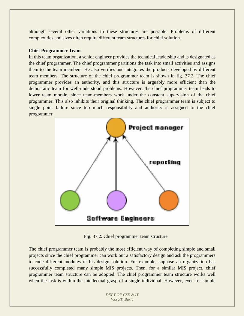
DEPT OF CSE & IT
VSSUT, Burla
although several other variations to these structures are possible. Problems of different
complexities and sizes often require different team structures for chief solution.
Chief Programmer Team
In this team organization, a senior engineer provides the technical leadership and is designated as
the chief programmer. The chief programmer partitions the task into small activities and assigns
them to the team members. He also verifies and integrates the products developed by different
team members. The structure of the chief programmer team is shown in fig. 37.2. The chief
programmer provides an authority, and this structure is arguably more efficient than the
democratic team for well-understood problems. However, the chief programmer team leads to
lower team morale, since team-members work under the constant supervision of the chief
programmer. This also inhibits their original thinking. The chief programmer team is subject to
single point failure since too much responsibility and authority is assigned to the chief
programmer.
Fig. 37.2: Chief programmer team structure
The chief programmer team is probably the most efficient way of completing simple and small
projects since the chief programmer can work out a satisfactory design and ask the programmers
to code different modules of his design solution. For example, suppose an organization has
successfully completed many simple MIS projects. Then, for a similar MIS project, chief
programmer team structure can be adopted. The chief programmer team structure works well
when the task is within the intellectual grasp of a single individual. However, even for simple
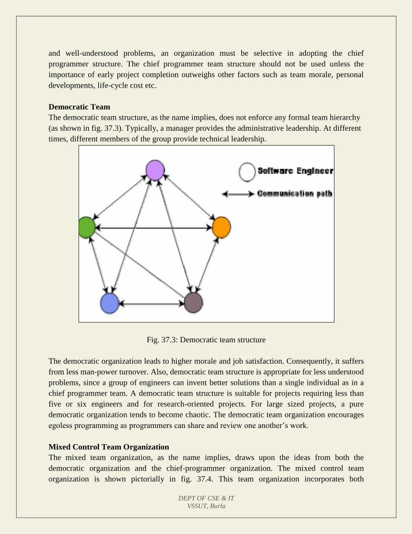
DEPT OF CSE & IT
VSSUT, Burla
and well-understood problems, an organization must be selective in adopting the chief
programmer structure. The chief programmer team structure should not be used unless the
importance of early project completion outweighs other factors such as team morale, personal
developments, life-cycle cost etc.
Democratic Team
The democratic team structure, as the name implies, does not enforce any formal team hierarchy
(as shown in fig. 37.3). Typically, a manager provides the administrative leadership. At different
times, different members of the group provide technical leadership.
Fig. 37.3: Democratic team structure
The democratic organization leads to higher morale and job satisfaction. Consequently, it suffers
from less man-power turnover. Also, democratic team structure is appropriate for less understood
problems, since a group of engineers can invent better solutions than a single individual as in a
chief programmer team. A democratic team structure is suitable for projects requiring less than
five or six engineers and for research-oriented projects. For large sized projects, a pure
democratic organization tends to become chaotic. The democratic team organization encourages
egoless programming as programmers can share and review one another’s work.
Mixed Control Team Organization
The mixed team organization, as the name implies, draws upon the ideas from both the
democratic organization and the chief-programmer organization. The mixed control team
organization is shown pictorially in fig. 37.4. This team organization incorporates both
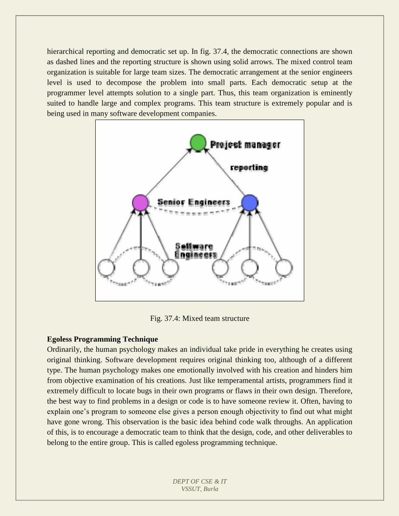
DEPT OF CSE & IT
VSSUT, Burla
hierarchical reporting and democratic set up. In fig. 37.4, the democratic connections are shown
as dashed lines and the reporting structure is shown using solid arrows. The mixed control team
organization is suitable for large team sizes. The democratic arrangement at the senior engineers
level is used to decompose the problem into small parts. Each democratic setup at the
programmer level attempts solution to a single part. Thus, this team organization is eminently
suited to handle large and complex programs. This team structure is extremely popular and is
being used in many software development companies.
Fig. 37.4: Mixed team structure
Egoless Programming Technique
Ordinarily, the human psychology makes an individual take pride in everything he creates using
original thinking. Software development requires original thinking too, although of a different
type. The human psychology makes one emotionally involved with his creation and hinders him
from objective examination of his creations. Just like temperamental artists, programmers find it
extremely difficult to locate bugs in their own programs or flaws in their own design. Therefore,
the best way to find problems in a design or code is to have someone review it. Often, having to
explain one’s program to someone else gives a person enough objectivity to find out what might
have gone wrong. This observation is the basic idea behind code walk throughs. An application
of this, is to encourage a democratic team to think that the design, code, and other deliverables to
belong to the entire group. This is called egoless programming technique.
DEPT OF CSE & IT
VSSUT, Burla
Characteristics of a good software engineer
The attributes that good software engineers should possess are as follows:
Exposure to systematic techniques, i.e. familiarity with software engineering principles.
Good technical knowledge of the project areas (Domain knowledge).
Good programming abilities.
Good communication skills. These skills comprise of oral, written, and interpersonal
skills.
High motivation.
Sound knowledge of fundamentals of computer science.
Intelligence.
Ability to work in a team
Discipline, etc.
Studies show that these attributes vary as much as 1:30 for poor and bright candidates. An
experiment conducted by Sackman [1968] shows that the ratio of coding hour for the worst to the
best programmers is 25:1, and the ratio of debugging hours is 28:1. Also, the ability of a software
engineer to arrive at the design of the software from a problem description varies greatly with
respect to the parameters of quality and time.
Technical knowledge in the area of the project (domain knowledge) is an important factor
determining the productivity of an individual for a particular project, and the quality of the
product that he develops. A programmer having a thorough knowledge of database application
(e.g. MIS) may turn out to be a poor data communication engineer. Lack of familiarity with the
application areas can result in low productivity and poor quality of the product.
Since software development is a group activity, it is vital for a software engineer to possess three
main kinds of communication skills: Oral, Written, and Interpersonal. A software engineer not
only needs to effectively communicate with his teammates (e.g. reviews, walk throughs, and
other team communications) but may also have to communicate with the customer to gather
product requirements. Poor interpersonal skills hamper these vital activities and often show up as
poor quality of the product and low productivity. Software engineers are also required at times to
make presentations to the managers and to the customers. This requires a different kind of
communication skill (oral communication skill). A software engineer is also expected to
document his work (design, code, test, etc.) as well as write the users’ manual, training manual,
installation manual, maintenance manual, etc. This requires good written communication skill.
Motivation level of software engineers is another crucial factor contributing to his work quality
and productivity. Even though no systematic studies have been reported in this regard, it is
generally agreed that even bright engineers may turn out to be poor performers when they have
lack motivation. An average engineer who can work with a single mind track can outperform
other engineers, higher incentives and better working conditions have only limited effect on their

DEPT OF CSE & IT
VSSUT, Burla
motivation levels. Motivation is to a great extent determined by personal traits, family and social
backgrounds, etc.
DEPT OF CSE & IT
VSSUT, Burla
LECTURE NOTE 38
RISK MANAGEMENT
A software project can be affected by a large variety of risks. In order to be able to
systematically identify the important risks which might affect a software project, it is necessary
to categorize risks into different classes. The project manager can then examine which risks from
each class are relevant to the project.
There are three main categories of risks which can affect a software project:
1. Project risks
Project risks concern varies forms of budgetary, schedule, personnel, resource, and
customer-related problems. An important project risk is schedule slippage. Since,
software is intangible, it is very difficult to monitor and control a software project. It is
very difficult to control something which cannot be seen. For any manufacturing project,
such as manufacturing of cars, the project manager can see the product taking shape. He
can for instance, see that the engine is fitted, after that the doors are fitted, the car is
getting painted, etc. Thus he can easily assess the progress of the work and control it. The
invisibility of the product being developed is an important reason why many software
projects suffer from the risk of schedule slippage.
2. Technical risks
Technical risks concern potential design, implementation, interfacing, testing, and
maintenance problems. Technical risks also include ambiguous specification, incomplete
specification, changing specification, technical uncertainty, and technical obsolescence.
Most technical risks occur due to the development team’s insufficient knowledge about
the project.
3. Business risks
This type of risks include risks of building an excellent product that no one wants, losing
budgetary or personnel commitments, etc.
Risk Assessment
The objective of risk assessment is to rank the risks in terms of their damage causing potential.
For risk assessment, first each risk should be rated in two ways:
• The likelihood of a risk coming true (denoted as r).
• The consequence of the problems associated with that risk (denoted as s).
DEPT OF CSE & IT
VSSUT, Burla
Based on these two factors, the priority of each risk can be computed:
p = r * s
Where, p is the priority with which the risk must be handled, r is the probability of the risk
becoming true, and s is the severity of damage caused due to the risk becoming true. If all
identified risks are prioritized, then the most likely and damaging risks can be handled first and
more comprehensive risk abatement procedures can be designed for these risks.
Risk Containment
After all the identified risks of a project are assessed, plans must be made to contain the most
damaging and the most likely risks. Different risks require different containment procedures. In
fact, most risks require ingenuity on the part of the project manager in tackling the risk.
There are three main strategies to plan for risk containment:
Avoid the risk- This may take several forms such as discussing with the customer to change the
requirements to reduce the scope of the work, giving incentives to the engineers to avoid the risk
of manpower turnover, etc.
Transfer the risk- This strategy involves getting the risky component developed by a third
party, buying insurance cover, etc.
Risk reduction- This involves planning ways to contain the damage due to a risk. For example,
if there is risk that some key personnel might leave, new recruitment may be planned.
Risk Leverage
To choose between the different strategies of handling a risk, the project manager must consider
the cost of handling the risk and the corresponding reduction of risk. For this the risk leverage of
the different risks can be computed.
Risk leverage is the difference in risk exposure divided by the cost of reducing the risk. More
formally,
risk leverage = (risk exposure before reduction – risk exposure after reduction) / (cost
of reduction)
Risk related to schedule slippage
Even though there are three broad ways to handle any risk, but still risk handling requires a lot of
ingenuity on the part of a project manager. As an example, it can be considered the options
available to contain an important type of risk that occurs in many software projects – that of
schedule slippage. Risks relating to schedule slippage arise primarily due to the intangible nature
DEPT OF CSE & IT
VSSUT, Burla
of software. Therefore, these can be dealt with by increasing the visibility of the software
product. Visibility of a software product can be increased by producing relevant documents
during the development process wherever meaningful and getting these documents reviewed by
an appropriate team. Milestones should be placed at regular intervals through a software
engineering process to provide a manager with regular indication of progress. Completion of a
phase of the development process before followed need not be the only milestones. Every phase
can be broken down to reasonable-sized tasks and milestones can be scheduled for these tasks
too. A milestone is reached, once documentation produced as part of a software engineering task
is produced and gets successfully reviewed. Milestones need not be placed for every activity. An
approximate rule of thumb is to set a milestone every 10 to 15 days.
Software Configuration Management
The results (also called as the deliverables) of a large software development effort typically
consist of a large number of objects, e.g. source code, design document, SRS document, test
document, user’s manual, etc. These objects are usually referred to and modified by a number of
software engineers through out the life cycle of the software. The state of all these objects at any
point of time is called the configuration of the software product. The state of each deliverable
object changes as development progresses and also as bugs are detected and fixed.
Release vs. Version vs. Revision
A new version of a software is created when there is a significant change in functionality,
technology, or the hardware it runs on, etc. On the other hand a new revision of a software refers
to minor bug fix in that software. A new release is created if there is only a bug fix, minor
enhancements to the functionality, usability, etc.
For example, one version of a mathematical computation package might run on Unix-based
machines, another on Microsoft Windows and so on. As a software is released and used by the
customer, errors are discovered that need correction. Enhancements to the functionalities of the
software may also be needed. A new release of software is an improved system intended to
replace an old one. Often systems are described as version m, release n; or simple m.n. Formally,
a history relation is version of can be defined between objects. This relation can be split into two
sub relations is revision of and is variant of.
Necessity of software configuration management
There are several reasons for putting an object under configuration management. But, possibly
the most important reason for configuration management is to control the access to the different
deliverable objects. Unless strict discipline is enforced regarding updation and storage of
different objects, several problems appear. The following are some of the important problems
that appear if configuration management is not used.
DEPT OF CSE & IT
VSSUT, Burla
Inconsistency problem when the objects are replicated. A scenario can be considered
where every software engineer has a personal copy of an object (e.g. source code). As
each engineer makes changes to his local copy, he is expected to intimate them to other
engineers, so that the changes in interfaces are uniformly changed across all modules.
However, many times an engineer makes changes to the interfaces in his local copies and
forgets to intimate other teammates about the changes. This makes the different copies of
the object inconsistent. Finally, when the product is integrated, it does not work.
Therefore, when several team members work on developing an object, it is necessary for
them to work on a single copy of the object, otherwise inconsistency may arise.
Problems associated with concurrent access. Suppose there is a single copy of a
problem module, and several engineers are working on it. Two engineers may
simultaneously carry out changes to different portions of the same module, and while
saving overwrite each other. Though the problem associated with concurrent access to
program code has been explained, similar problems occur for any other deliverable
object.
Providing a stable development environment. When a project is underway, the team
members need a stable environment to make progress. Suppose somebody is trying to
integrate module A, with the modules B and C, he cannot make progress if developer of
module C keeps changing C; this can be especially frustrating if a change to module C
forces him to recompile A. When an effective configuration management is in place, the
manager freezes the objects to form a base line. When anyone needs any of the objects
under configuration control, he is provided with a copy of the base line item. The
requester makes changes to his private copy. Only after the requester is through with all
modifications to his private copy, the configuration is updated and a new base line gets
formed instantly. This establishes a baseline for others to use and depend on. Also,
configuration may be frozen periodically. Freezing a configuration may involve archiving
everything needed to rebuild it. (Archiving means copying to a safe place such as a
magnetic tape).
System accounting and maintaining status information. System accounting keeps
track of who made a particular change and when the change was made.
Handling variants. Existence of variants of a software product causes some peculiar
problems. Suppose somebody has several variants of the same module, and finds a bug in
one of them. Then, it has to be fixed in all versions and revisions. To do it efficiently, he
should not have to fix it in each and every version and revision of the software separately.
DEPT OF CSE & IT
VSSUT, Burla
Software Configuration Management Activities
Normally, a project manager performs the configuration management activity by using an
automated configuration management tool. A configuration management tool provides
automated support for overcoming all the problems mentioned above. In addition, a
configuration management tool helps to keep track of various deliverable objects, so that the
project manager can quickly and unambiguously determine the current state of the project. The
configuration management tool enables the engineers to change the various components in a
controlled manner.
Configuration management is carried out through two principal activities:
• Configuration identification involves deciding which parts of the system should be kept
track of.
• Configuration control ensures that changes to a system happen smoothly.
Configuration Identification
The project manager normally classifies the objects associated with a software development
effort into three main categories: controlled, pre controlled, and uncontrolled. Controlled objects
are those which are already put under configuration control. One must follow some formal
procedures to change them. Pre controlled objects are not yet under configuration control, but
will eventually be under configuration control. Uncontrolled objects are not and will not be
subjected to configuration control. Controllable objects include both controlled and pre
controlled objects. Typical controllable objects include:
• Requirements specification document
• Design documents
Tools used to build the system, such as compilers, linkers, lexical analyzers, parsers, etc.
• Source code for each module
• Test cases
• Problem reports
The configuration management plan is written during the project planning phase and it lists all
controlled objects. The managers who develop the plan must strike a balance between controlling
too much, and controlling too little. If too much is controlled, overheads due to configuration
management increase to unreasonably high levels. On the other hand, controlling too little might
lead to confusion when something changes.
Configuration Control
Configuration control is the process of managing changes to controlled objects. Configuration
control is the part of a configuration management system that most directly affects the day-to-
day operations of developers. The configuration control system prevents unauthorized changes to

DEPT OF CSE & IT
VSSUT, Burla
any controlled objects. In order to change a controlled object such as a module, a developer can
get a private copy of the module by a reserve operation as shown in fig. 38.1. Configuration
management tools allow only one person to reserve a module at a time. Once an object is
reserved, it does not allow anyone else to reserve this module until the reserved module is
restored as shown in fig. 38.1. Thus, by preventing more than one engineer to simultaneously
reserve a module, the problems associated with concurrent access are solved.
Fig. 38.1: Reserve and restore operation in configuration control
It can be shown how the changes to any object that is under configuration control can be
achieved. The engineer needing to change a module first obtains a private copy of the module
through a reserve operation. Then, he carries out all necessary changes on this private copy.
However, restoring the changed module to the system configuration requires the permission of a
change control board (CCB). The CCB is usually constituted from among the development team
members. For every change that needs to be carried out, the CCB reviews the changes made to
the controlled object and certifies several things about the change:
1. Change is well-motivated.
2. Developer has considered and documented the effects of the change.
3. Changes interact well with the changes made by other developers.
4. Appropriate people (CCB) have validated the change, e.g. someone has tested the changed
code, and has verified that the change is consistent with the requirement.
DEPT OF CSE & IT
VSSUT, Burla
The change control board (CCB) sounds like a group of people. However, except for very
large projects, the functions of the change control board are normally discharged by the
project manager himself or some senior member of the development team. Once the CCB
reviews the changes to the module, the project manager updates the old base line through a
restore operation (as shown in fig. 38.1). A configuration control tool does not allow a
developer to replace an object he has reserved with his local copy unless he gets an
authorization from the CCB. By constraining the developers’ ability to replace reserved
objects, a stable environment is achieved. Since a configuration management tool allows only
one engineer to work on one module at any one time, problem of accidental overwriting is
eliminated. Also, since only the manager can update the baseline after the CCB approval,
unintentional changes are eliminated.
Configuration Management Tools
SCCS and RCS are two popular configuration management tools available on most UNIX
systems. SCCS or RCS can be used for controlling and managing different versions of text files.
SCCS and RCS do not handle binary files (i.e. executable files, documents, files containing
diagrams, etc.) SCCS and RCS provide an efficient way of storing versions that minimizes the
amount of occupied disk space. Suppose, a module MOD is present in three versions MOD1.1,
MOD1.2, and MOD1.3. Then, SCCS and RCS stores the original module MOD1.1 together with
changes needed to transform MOD1.1 into MOD1.2 and MOD1.2 to MOD1.3. The changes
needed to transform each base lined file to the next version are stored and are called deltas. The
main reason behind storing the deltas rather than storing the full version files is to save disk
space. The change control facilities provided by SCCS and RCS include the ability to
incorporate restrictions on the set of individuals who can create new versions, and facilities for
checking components in and out (i.e. reserve and restore operations). Individual developers
check out components and modify them. After they have made all necessary changes to a module
and after the changes have been reviewed, they check in the changed module into SCCS or RCS.
Revisions are denoted by numbers in ascending order, e.g., 1.1, 1.2, 1.3 etc. It is also possible to
create variants or revisions of a component by creating a fork in the development history.
DEPT OF CSE & IT
VSSUT, Burla
LECTURE NOTE 39
COMPUTER AIDED SOFTWARE ENGINEERING
CASE tool and its scope
A CASE (Computer Aided Software Engineering) tool is a generic term used to denote any form
of automated support for software engineering. In a more restrictive sense, a CASE tool means
any tool used to automate some activity associated with software development. Many CASE
tools are available. Some of these CASE tools assist in phase related tasks such as specification,
structured analysis, design, coding, testing, etc.; and others to non-phase activities such as project
management and configuration management.
Reasons for using CASE tools
The primary reasons for using a CASE tool are:
• To increase productivity
• To help produce better quality software at lower cost
CASE environment
Although individual CASE tools are useful, the true power of a tool set can be realized only
when these set of tools are integrated into a common framework or environment. CASE tools are
characterized by the stage or stages of software development life cycle on which they focus.
Since different tools covering different stages share common information, it is required that they
integrate through some central repository to have a consistent view of information associated
with the software development artifacts. This central repository is usually a data dictionary
containing the definition of all composite and elementary
data items. Through the central repository all the CASE tools in a CASE environment share
common information among themselves. Thus a CASE environment facilities the automation of
the step-by-step methodologies for software development. A schematic representation of a CASE
environment is shown in fig. 39.1.
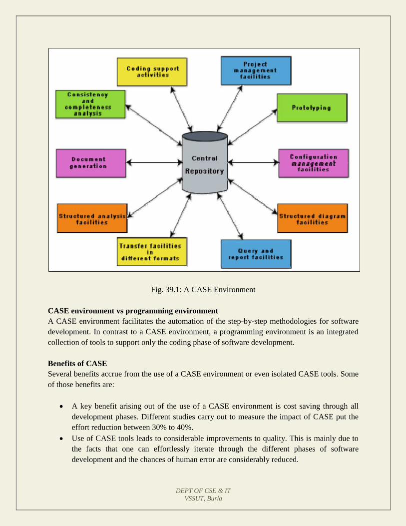
DEPT OF CSE & IT
VSSUT, Burla
Fig. 39.1: A CASE Environment
CASE environment vs programming environment
A CASE environment facilitates the automation of the step-by-step methodologies for software
development. In contrast to a CASE environment, a programming environment is an integrated
collection of tools to support only the coding phase of software development.
Benefits of CASE
Several benefits accrue from the use of a CASE environment or even isolated CASE tools. Some
of those benefits are:
A key benefit arising out of the use of a CASE environment is cost saving through all
development phases. Different studies carry out to measure the impact of CASE put the
effort reduction between 30% to 40%.
Use of CASE tools leads to considerable improvements to quality. This is mainly due to
the facts that one can effortlessly iterate through the different phases of software
development and the chances of human error are considerably reduced.
DEPT OF CSE & IT
VSSUT, Burla
CASE tools help produce high quality and consistent documents. Since the important
data relating to a software product are maintained in a central repository, redundancy in
the stored data is reduced and therefore chances of inconsistent documentation is reduced
to a great extent.
CASE tools take out most of the drudgery in a software engineer’s work. For example,
they need not check meticulously the balancing of the DFDs but can do it effortlessly
through the press of a button.
CASE tools have led to revolutionary cost saving in software maintenance efforts. This
arises not only due to the tremendous value of a CASE environment in traceability and
consistency checks, but also due to the systematic information capture during the various
phases of software development as a result of adhering to a CASE environment.
Introduction of a CASE environment has an impact on the style of working of a
company, and makes it oriented towards the structured and orderly approach.
Requirements of a prototyping CASE tool
Prototyping is useful to understand the requirements of complex software products, to
demonstrate a concept, to market new ideas, and so on. The important features of a prototyping
CASE tool are as follows:
• Define user interaction
• Define the system control flow
• Store and retrieve data required by the system
• Incorporate some processing logic
Features of a good prototyping CASE tool
There are several stand-alone prototyping tools. But a tool that integrates with the data dictionary
can make use of the entries in the data dictionary, help in populating the data dictionary and
ensure the consistency between the design data and the prototype. A good prototyping tool
should support the following features:
Since one of the main uses of a prototyping CASE tool is graphical user interface (GUI)
development, prototyping CASE tool should support the user to create a GUI using a
graphics editor. The user should be allowed to define all data entry forms, menus and
controls.
It should integrate with the data dictionary of a CASE environment.
If possible, it should be able to integrate with external user defined modules written in C
or some popular high level programming languages.
The user should be able to define the sequence of states through which a created
prototype can run. The user should also be allowed to control the running of the
prototype.
DEPT OF CSE & IT
VSSUT, Burla
The run time system of prototype should support mock runs of the actual system and
management of the input and output data.
Structured analysis and design with CASE tools
Several diagramming techniques are used for structured analysis and structured design. The
following supports might be available from CASE tools.
A CASE tool should support one or more of the structured analysis and design
techniques.
It should support effortlessly drawing analysis and design diagrams.
It should support drawing for fairly complex diagrams, preferably through a hierarchy of
levels.
The CASE tool should provide easy navigation through the different levels and through
the design and analysis.
The tool must support completeness and consistency checking across the design and
analysis and through all levels of analysis hierarchy. Whenever it is possible, the system
should disallow any inconsistent operation, but it may be very difficult to implement such
a feature. Whenever there arises heavy computational load while consistency checking, it
should be possible to temporarily disable consistency checking.
Code generation and CASE tools
As far as code generation is concerned, the general expectation of a CASE tool is quite low. A
reasonable requirement is traceability from source file to design data. More pragmatic supports
expected from a CASE tool during code generation phase are the following:
The CASE tool should support generation of module skeletons or templates in one or
more popular languages. It should be possible to include copyright message, brief
description of the module, author name and the date of creation in some selectable
format.
The tool should generate records, structures, class definition automatically from the
contents of the data dictionary in one or more popular languages.
It should generate database tables for relational database management systems.
The tool should generate code for user interface from prototype definition for X window
and MS window based applications.
Test case generation CASE tool
The CASE tool for test case generation should have the following features:
It should support both design and requirement testing.
It should generate test set reports in ASCII format which can be directly imported into the
test plan document.
DEPT OF CSE & IT
VSSUT, Burla
Hardware and environmental requirements
In most cases, it is the existing hardware that would place constraints upon the CASE tool
selection. Thus, instead of defining hardware requirements for a CASE tool, the task at hand
becomes to fit in an optimal configuration of CASE tool in the existing hardware capabilities.
Therefore, it can be emphasized on selecting the most optimal CASE tool configuration for a
given hardware configuration.
The heterogeneous network is one instance of distributed environment and this can be chosen for
illustration as it is more popular due to its machine independent features. The CASE tool
implementation in heterogeneous network makes use of client-server paradigm. The multiple
clients who run different modules access data dictionary through this server. The data dictionary
server may support one or more projects. Though it is possible to run many servers for different
projects but distributed implementation of data dictionary is not common.
The tool set is integrated through the data dictionary which supports multiple projects, multiple
users working simultaneously and allows sharing information between users and projects. The
data dictionary provides consistent view of all project entities, e.g. a data record definition and its
entity-relationship diagram be consistent. The server should depict the per-project logical view
of the data dictionary. This means that it should allow back up/restore, copy, cleaning part of the
data dictionary, etc.
The tool should work satisfactorily for maximum possible number of users working
simultaneously. The tool should support multi-windowing environment for the users. This is
important to enable the users to see more than one diagram at a time. It also facilitates navigation
and switching from one part to the other.
Documentation Support
The deliverable documents should be organized graphically and should be able to incorporate
text and diagrams from the central repository. This helps in producing up-to-date documentation.
The CASE tool should integrate with one or more of the commercially available desktop
publishing packages. It should be possible to export text, graphics, tables, data dictionary reports
to the DTP package in standard forms such as PostScript.
Project Management Support
The CASE tool should support collecting, storing, and analyzing information on the software
project’s progress such as the estimated task duration, scheduled and actual task start, completion
date, dates and results of the reviews, etc.
DEPT OF CSE & IT
VSSUT, Burla
External Interface
The CASE tool should allow exchange of information for reusability of design. The information
which is to be exported by the CASE tool should be preferably in ASCII format and support
open architecture. Similarly, the data dictionary should provide a programming interface to
access information. It is required for integration of custom utilities, building new techniques, or
populating the data dictionary.
Reverse Engineering
The CASE tool should support generation of structure charts and data dictionaries from the
existing source codes. It should populate the data dictionary from the source code. If the tool is
used for re-engineering information systems, it should contain conversion tool from indexed
sequential file structure, hierarchical and network database to relational database systems.
Data Dictionary Interface
The data dictionary interface should provide view and update access to the entities and relations
stored in it. It should have print facility to obtain hard copy of the viewed screens. It should
provide analysis reports like cross-referencing, impact analysis, etc. Ideally, it should support a
query language to view its contents.
Second-generation CASE tool
An important feature of the second-generation CASE tool is the direct support of any adapted
methodology. This would necessitate the function of a CASE administrator organization who can
tailor the CASE tool to a particular methodology. In addition, the second-generation CASE tools
have following features:
Intelligent diagramming support- The fact that diagramming techniques are useful for
system analysis and design is well established. The future CASE tools would provide
help to aesthetically and automatically lay out the diagrams.
Integration with implementation environment- The CASE tools should provide
integration between design and implementation.
Data dictionary standards- The user should be allowed to integrate many development
tools into one environment. It is highly unlikely that any one vendor will be able to
deliver a total solution. Moreover, a preferred tool would require tuning up for a
particular system. Thus the user would act as a system integrator. This is possibly only if
some standard on data dictionary emerges.
Customization support- The user should be allowed to define new types of objects and
connections. This facility may be used to build some special methodologies. Ideally it
should be possible to specify the rules of a methodology to a rule engine for carrying out
the necessary consistency checks.
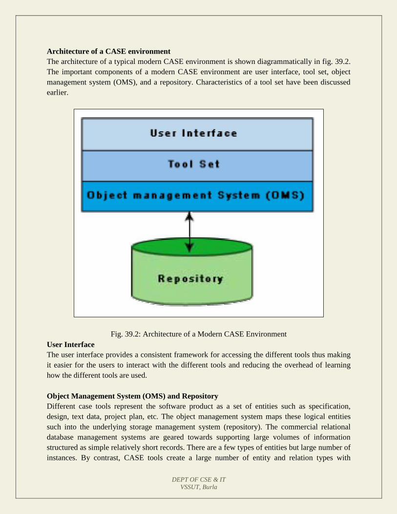
DEPT OF CSE & IT
VSSUT, Burla
Architecture of a CASE environment
The architecture of a typical modern CASE environment is shown diagrammatically in fig. 39.2.
The important components of a modern CASE environment are user interface, tool set, object
management system (OMS), and a repository. Characteristics of a tool set have been discussed
earlier.
Fig. 39.2: Architecture of a Modern CASE Environment
User Interface
The user interface provides a consistent framework for accessing the different tools thus making
it easier for the users to interact with the different tools and reducing the overhead of learning
how the different tools are used.
Object Management System (OMS) and Repository
Different case tools represent the software product as a set of entities such as specification,
design, text data, project plan, etc. The object management system maps these logical entities
such into the underlying storage management system (repository). The commercial relational
database management systems are geared towards supporting large volumes of information
structured as simple relatively short records. There are a few types of entities but large number of
instances. By contrast, CASE tools create a large number of entity and relation types with

DEPT OF CSE & IT
VSSUT, Burla
perhaps a few instances of each. Thus the object management system takes care of appropriately
mapping into the underlying storage management system.
DEPT OF CSE & IT
VSSUT, Burla
LECTURE NOTE 40
SOFTWARE REUSE
Advantages of software reuse
Software products are expensive. Software project managers are worried about the high cost of
software development and are desperately look for ways to cut development cost. A possible
way to reduce development cost is to reuse parts from previously developed software. In addition
to reduced development cost and time, reuse also leads to higher quality of the developed
products since the reusable components are ensured to have high quality.
Artifacts that can be reused
It is important to know about the kinds of the artifacts associated with software development that
can be reused. Almost all artifacts associated with software development, including project plan
and test plan can be reused. However, the prominent items that can be effectively reused are:
• Requirements specification
• Design
• Code
• Test cases
• Knowledge
Pros and cons of knowledge reuse
Knowledge is the most abstract development artifact that can be reused. Out of all the reuse
artifacts i.e. requirements specification, design, code, test cases, reuse of knowledge occurs
automatically without any conscious effort in this direction. However, two major difficulties with
unplanned reuse of knowledge are that a developer experienced in one type of software product
might be included in a team developing a different type of software. Also, it is difficult to
remember the details of the potentially reusable development knowledge. A planned reuse of
knowledge can increase the effectiveness of reuse. For this, the reusable knowledge should be
systematically extracted and documented. But, it is usually very difficult to extract and document
reusable knowledge.
Easiness of reuse of mathematical functions
The routines of mathematical libraries are being reused very successfully by almost every
programmer. No one in his right mind would think of writing a routine to compute sine or
cosine. Reuse of commonly used mathematical functions is easy. Several interesting aspects
emerge. Cosine means the same to all. Everyone has clear ideas about what kind of argument
should cosine take, the type of processing to be carried out and the results returned. Secondly,
DEPT OF CSE & IT
VSSUT, Burla
mathematical libraries have a small interface. For example, cosine requires only one parameter.
Also, the data formats of the parameters are standardized.
Basic issues in any reuse program
The following are some of the basic issues that must be clearly understood for starting any reuse
program.
• Component creation
• Component indexing and storing
• Component search
• Component understanding
• Component adaptation
• Repository maintenance
Component creation- For component creation, the reusable components have to be first
identified. Selection of the right kind of components having potential for reuse is important.
Domain analysis is a promising technique which can be used to create reusable components.
Component indexing and storing- Indexing requires classification of the reusable
components so that they can be easily searched when looking for a component for reuse. The
components need to be stored in a Relational Database Management System (RDBMS) or an
Object-Oriented Database System (ODBMS) for efficient access when the number of
components becomes large.
Component searching- The programmers need to search for right components matching
their requirements in a database of components. To be able to search components efficiently,
the programmers require a proper method to describe the components that they are looking
for.
Component understanding- The programmers need a precise and sufficiently complete
understanding of what the component does to be able to decide whether they can reuse the
component. To facilitate understanding, the components should be well documented and
should do something simple.
Component adaptation- Often, the components may need adaptation before they can be
reused, since a selected component may not exactly fit the problem at hand. However,
tinkering with the code is also not a satisfactory solution because this is very likely to be a
source of bugs.
Repository maintenance- A component repository once is created requires continuous
maintenance. New components, as and when created have to be entered into the repository.
DEPT OF CSE & IT
VSSUT, Burla
The faulty components have to be tracked. Further, when new applications emerge, the older
applications become obsolete. In this case, the obsolete components might have to be
removed from the repository.
Domain Analysis
The aim of domain analysis is to identify the reusable components for a problem domain.
Reuse domain- A reuse domain is a technically related set of application areas. A body of
information is considered to be a problem domain for reuse, if a deep and comprehensive
relationship exists among the information items as categorized by patterns of similarity among
the development components of the software product. A reuse domain is shared understanding of
some community, characterized by concepts, techniques, and terminologies that show some
coherence. Examples of domains are accounting software domain, banking software domain,
business software domain, manufacturing automation software domain, telecommunication
software domain, etc.
Just to become familiar with the vocabulary of a domain requires months of interaction with the
experts. Often, one needs to be familiar with a network of related domains for successfully
carrying out domain analysis. Domain analysis identifies the objects, operations, and the
relationships among them. For example, consider the airline reservation system, the reusable
objects can be seats, flights, airports, crew, meal orders, etc. The reusable operations can be
scheduling a flight, reserving a seat, assigning crew to flights, etc. The domain analysis
generalizes the application domain. A domain model transcends specific applications. The
common characteristics or the similarities between systems are generalized.
During domain analysis, a specific community of software developers gets together to discuss
community-wide-solutions. Analysis of the application domain is required to identify the
reusable components. The actual construction of reusable components for a domain is called
domain engineering.
Evolution of a reuse domain- The ultimate result of domain analysis is development of
problem-oriented languages. The problem-oriented languages are also known as application
generators. These application generators, once developed form application development
standards. The domains slowly develop. As a domain develops, it is distinguishable the various
stages it undergoes:
Stage 1: There is no clear and consistent set of notations. Obviously, no reusable components are
available. All software is written from scratch.
Stage 2: Here, only experience from similar projects is used in a development effort. This means
that there is only knowledge reuse.

DEPT OF CSE & IT
VSSUT, Burla
Stage 3: At this stage, the domain is ripe for reuse. The set of concepts are stabilized and the
notations standardized. Standard solutions to standard problems are available. There is both
knowledge and component reuse.
Stage 4: The domain has been fully explored. The software development for the domain can be
largely automated. Programs are not written in the traditional sense any more. Programs are
written using a domain specific language, which is also known as an application generator.
DEPT OF CSE & IT
VSSUT, Burla
LECTURE NOTE 41
REUSE APPROACH
Components Classification
Components need to be properly classified in order to develop an effective indexing and storage
scheme. Hardware reuse has been very successful. Hardware components are classified using a
multilevel hierarchy. At the lowest level, the components are described in several forms: natural
language description, logic schema, timing information, etc. The higher the level at which a
component is described, the more is the ambiguity. This has motivated the Prieto-Diaz’s
classification scheme.
Prieto-Diaz’s classification scheme: Each component is best described using a number of
different characteristics or facets. For example, objects can be classified using the following:
Searching- The domain repository may contain thousands of reuse items. A popular search
technique that has proved to be very effective is one that provides a web interface to the
repository. Using such a web interface, one would search an item using an approximate
automated search using key words, and then from these results do a browsing using the links
provided to look up related items. The approximate automated search locates products that
appear to fulfill some of the specified requirements. The items located through the approximate
search serve as a starting point for browsing the repository. These serve as the starting point for
browsing the repository. The developer may follow links to other products until a sufficiently
good match is found. Browsing is done using the keyword-to-keyword, keyword-to-product, and
product-to-product links. These links help to locate additional products and compare their
detailed attributes. Finding a satisfactorily item from the repository may require several locations
of approximate search followed by browsing. With each iteration, the developer would get a
better understanding of the available products and their differences. However, we must
remember that the items to be searched may be components, designs, models, requirements, and
even knowledge.
Repository maintenance - Repository maintenance involves entering new items, retiring those
items which are no more necessary, and modifying the search attributes of items to improve the
effectiveness of search. The software industry is always trying to implement something that has
not been quite done before. As patterns requirements emerge, new reusable components are
identified, which may ultimately become more or less the standards. However, as technology
advances, some components which are still reusable, do not fully address the current
requirements. On the other hand, restricting reuse to highly mature components, sacrifices one of
that creates potential reuse opportunity. Making a product available before it has been thoroughly
DEPT OF CSE & IT
VSSUT, Burla
assessed can be counter productive. Negative experiences tend to dissolve the trust in the entire
reuse framework.
Application generator -The problem- oriented languages are known as application generators.
Application generators translate specifications into application programs. The specification is
usually written using 4GL. The specification might also in a visual form. Application generator
can be applied successfully to data processing application, user interface, and compiler
development.
Advantages of application generators
Application generators have significant advantages over simple parameterized programs. The
biggest of these is that the application generators can express the variant information in an
appropriate language rather than being restricted to function parameters, named constants, or
tables. The other advantages include fewer errors, easier to maintain, substantially reduced
development effort, and the fact that one need not bother about the implementation details.
Shortcomings of application generators
Application generators are handicapped when it is necessary to support some new concepts or
features. Application generators are less successful with the development of applications with
close interaction with hardware such as real-time systems.
Re-use at organization level
Achieving organization-level reuse requires adoption of the following steps:
• Assessing a product’s potential for reuse
• Refining products for greater reusability
• Entering the product in the reuse repository
Assessing a product’s potential for reuse. Assessment of components reuse potential
can be obtained from an analysis of a questionnaire circulated among the developers. The
questionnaire can be devised to access a component’s reusability. The programmers
working in similar application domain can be used to answer the questionnaire about the
product’s reusability. Depending on the answers given by the programmers, either the
component be taken up for reuse as it is, it is modified and refined before it is entered
into the reuse repository, or it is ignored. A sample questionnaire to assess a component’s
reusability is the following.
• Is the component’s functionality required for implementation of systems in the
future?
• How common is the component’s function within its domain?
• Would there be a duplication of functions within the domain if the component is
taken up?
DEPT OF CSE & IT
VSSUT, Burla
• Is the component hardware dependent?
• Is the design of the component optimized enough?
• If the component is non-reusable, then can it be decomposed to yield some reusable
components?
Can we parameterize a non-reusable component so that it becomes reusable?
Refining products for greater reusability. For a product to be reusable, it must be
relatively easy to adapt it to different contexts. Machine dependency must be abstracted
out or localized using data encapsulation techniques. The following refinements may be
carried out:
• Name generalization: The names should be general, rather than being directly
related to a specific application.
• Operation generalization: Operations should be added to make the component
more general. Also, operations that are too specific to an application can be removed.
• Exception generalization: This involves checking each component to see which
exceptions it might generate. For a general component, several types of exceptions
might have to be handled.
• Handling portability problems: Programs typically make some assumption
regarding the representation of information in the underlying machine. These
assumptions are in general not true for all machines. The programs also often need to
call some operating system functionality and these calls may not be same on all
machines. Also, programs use some function libraries, which may not be available on
all host machines. A portability solution to overcome these problems is shown in fig.
41.1. The portability solution suggests that rather than call the operating system and
I/O procedures directly, abstract versions of these should be called by the application
program. Also, all platform-related calls should be routed through the portability
interface. One problem with this solution is the significant overhead incurred, which
makes it inapplicable to many real-time systems and applications requiring very fast
response.

DEPT OF CSE & IT
VSSUT, Burla
Fig. 41.1: Improving reusability of a component by using a portability interface
Factors that inhibit an effective reuse program
In spite of all the shortcomings of the state-of-the-art reuse techniques, it is the experience of
several organizations that most of the factors inhibiting an effective reuse program are non-
technical. Some of these factors are the following.
Need for commitment from the top management.
Adequate documentation to support reuse.
Adequate incentive to reward those who reuse. Both the people contributing new reusable
components and those reusing the existing components should be rewarded to start a
reuse program and keep it going.
Providing access to and information about reusable components. Organizations are often
hesitant to provide an open access to the reuse repository for the fear of the reuse
components finding a way to their competitors.
DEPT OF CSE & IT
VSSUT, Burla
REFERENCES
BIBLIOGRAPHY
1. “Fundamentals of Software Engineering”, Rajib Mall, Prentice-Hall of India.
WEBLIOGRAPGY
2. http://www.tutorialspoint.com/