Embed Size (px)
Citation preview
Lecture Notes onQuantum Algorithms
Andrew M. Childs
Department of Computer Science,Institute for Advanced Computer Studies, and
Joint Center for Quantum Information and Computer Science
University of Maryland
30 May 2017

ii

Contents
Preface vii
1 Preliminaries 11.1 Quantum data . . . . . . . . . . . . . . . . . . . . . . . . . . . . . . . . . . . . . . . . . . . . 11.2 Quantum circuits . . . . . . . . . . . . . . . . . . . . . . . . . . . . . . . . . . . . . . . . . . . 11.3 Universal gate sets . . . . . . . . . . . . . . . . . . . . . . . . . . . . . . . . . . . . . . . . . . 21.4 Reversible computation . . . . . . . . . . . . . . . . . . . . . . . . . . . . . . . . . . . . . . . 21.5 Uniformity . . . . . . . . . . . . . . . . . . . . . . . . . . . . . . . . . . . . . . . . . . . . . . 31.6 Quantum complexity . . . . . . . . . . . . . . . . . . . . . . . . . . . . . . . . . . . . . . . . . 31.7 Fault tolerance . . . . . . . . . . . . . . . . . . . . . . . . . . . . . . . . . . . . . . . . . . . . 3
I Quantum circuits 5
2 Efficient universality of quantum circuits 72.1 Subadditivity of errors . . . . . . . . . . . . . . . . . . . . . . . . . . . . . . . . . . . . . . . . 72.2 The group commutator and a net around the identity . . . . . . . . . . . . . . . . . . . . . . 82.3 Proof of the Solovay-Kitaev Theorem . . . . . . . . . . . . . . . . . . . . . . . . . . . . . . . . 82.4 Proof of Lemma 2.3 . . . . . . . . . . . . . . . . . . . . . . . . . . . . . . . . . . . . . . . . . 9
3 Quantum circuit synthesis over Clifford+T 113.1 Converting to Matsumoto-Amano normal form . . . . . . . . . . . . . . . . . . . . . . . . . . 113.2 Uniqueness of Matsumoto-Amano normal form . . . . . . . . . . . . . . . . . . . . . . . . . . 123.3 Algebraic characterization of Clifford+T unitaries . . . . . . . . . . . . . . . . . . . . . . . . . 133.4 From exact to approximate synthesis . . . . . . . . . . . . . . . . . . . . . . . . . . . . . . . . 14
II Quantum algorithms for algebraic problems 15
4 The abelian quantum Fourier transform and phase estimation 174.1 Quantum Fourier transform . . . . . . . . . . . . . . . . . . . . . . . . . . . . . . . . . . . . . 174.2 QFT over Z2n . . . . . . . . . . . . . . . . . . . . . . . . . . . . . . . . . . . . . . . . . . . . . 174.3 Phase estimation . . . . . . . . . . . . . . . . . . . . . . . . . . . . . . . . . . . . . . . . . . . 194.4 QFT over ZN and over a general finite abelian group . . . . . . . . . . . . . . . . . . . . . . . 19
5 Discrete log and the hidden subgroup problem 215.1 Discrete log . . . . . . . . . . . . . . . . . . . . . . . . . . . . . . . . . . . . . . . . . . . . . . 215.2 Diffie-Hellman key exchange . . . . . . . . . . . . . . . . . . . . . . . . . . . . . . . . . . . . . 215.3 The hidden subgroup problem . . . . . . . . . . . . . . . . . . . . . . . . . . . . . . . . . . . . 225.4 Shor’s algorithm . . . . . . . . . . . . . . . . . . . . . . . . . . . . . . . . . . . . . . . . . . . 23
6 The abelian HSP and decomposing abelian groups 256.1 The abelian HSP . . . . . . . . . . . . . . . . . . . . . . . . . . . . . . . . . . . . . . . . . . . 256.2 Decomposing abelian groups . . . . . . . . . . . . . . . . . . . . . . . . . . . . . . . . . . . . . 27
7 Quantum attacks on elliptic curve cryptography 297.1 Elliptic curves . . . . . . . . . . . . . . . . . . . . . . . . . . . . . . . . . . . . . . . . . . . . . 297.2 Elliptic curve cryptography . . . . . . . . . . . . . . . . . . . . . . . . . . . . . . . . . . . . . 317.3 Shor’s algorithm for discrete log over elliptic curves . . . . . . . . . . . . . . . . . . . . . . . . 32
8 Quantum algorithms for number fields 33
iii

iv Contents
8.1 Review: Order finding . . . . . . . . . . . . . . . . . . . . . . . . . . . . . . . . . . . . . . . . 338.2 Pell’s equation . . . . . . . . . . . . . . . . . . . . . . . . . . . . . . . . . . . . . . . . . . . . 338.3 Some basic algebraic number theory . . . . . . . . . . . . . . . . . . . . . . . . . . . . . . . . 348.4 A periodic function for the units of Z[
√d] . . . . . . . . . . . . . . . . . . . . . . . . . . . . . 35
9 Period finding from Z to R 379.1 Period finding over the integers . . . . . . . . . . . . . . . . . . . . . . . . . . . . . . . . . . . 379.2 Period finding over the reals . . . . . . . . . . . . . . . . . . . . . . . . . . . . . . . . . . . . . 399.3 Other algorithms for number fields . . . . . . . . . . . . . . . . . . . . . . . . . . . . . . . . . 41
10 Quantum query complexity of the HSP 4310.1 The nonabelian HSP and its applications . . . . . . . . . . . . . . . . . . . . . . . . . . . . . 4310.2 The standard method . . . . . . . . . . . . . . . . . . . . . . . . . . . . . . . . . . . . . . . . 4410.3 Query complexity of the HSP . . . . . . . . . . . . . . . . . . . . . . . . . . . . . . . . . . . . 45
11 Fourier analysis in nonabelian groups 4711.1 A brief introduction to representation theory . . . . . . . . . . . . . . . . . . . . . . . . . . . 4711.2 Fourier analysis for nonabelian groups . . . . . . . . . . . . . . . . . . . . . . . . . . . . . . . 49
12 Fourier sampling 5112.1 Weak Fourier sampling . . . . . . . . . . . . . . . . . . . . . . . . . . . . . . . . . . . . . . . . 5112.2 Normal subgroups . . . . . . . . . . . . . . . . . . . . . . . . . . . . . . . . . . . . . . . . . . 5212.3 Strong Fourier sampling . . . . . . . . . . . . . . . . . . . . . . . . . . . . . . . . . . . . . . . 53
13 Kuperberg’s algorithm for the dihedral HSP 5513.1 The HSP in the dihedral group . . . . . . . . . . . . . . . . . . . . . . . . . . . . . . . . . . . 5513.2 Fourier sampling in the dihedral group . . . . . . . . . . . . . . . . . . . . . . . . . . . . . . . 5613.3 Combining states . . . . . . . . . . . . . . . . . . . . . . . . . . . . . . . . . . . . . . . . . . . 5613.4 The Kuperberg sieve . . . . . . . . . . . . . . . . . . . . . . . . . . . . . . . . . . . . . . . . . 5713.5 Analysis of the Kuperberg sieve . . . . . . . . . . . . . . . . . . . . . . . . . . . . . . . . . . . 5713.6 Entangled measurements . . . . . . . . . . . . . . . . . . . . . . . . . . . . . . . . . . . . . . . 58
14 The HSP in the Heisenberg group 5914.1 The Heisenberg group . . . . . . . . . . . . . . . . . . . . . . . . . . . . . . . . . . . . . . . . 5914.2 Fourier sampling . . . . . . . . . . . . . . . . . . . . . . . . . . . . . . . . . . . . . . . . . . . 6014.3 Two states are better than one . . . . . . . . . . . . . . . . . . . . . . . . . . . . . . . . . . . 60
15 Approximating the Jones polynomial 6315.1 The Hadamard test . . . . . . . . . . . . . . . . . . . . . . . . . . . . . . . . . . . . . . . . . . 6315.2 The Jones polynomial . . . . . . . . . . . . . . . . . . . . . . . . . . . . . . . . . . . . . . . . 6315.3 Links from braids . . . . . . . . . . . . . . . . . . . . . . . . . . . . . . . . . . . . . . . . . . . 6415.4 Representing braids in the Temperley-Lieb algebra . . . . . . . . . . . . . . . . . . . . . . . . 6415.5 A quantum algorithm . . . . . . . . . . . . . . . . . . . . . . . . . . . . . . . . . . . . . . . . 6515.6 Quality of approximation . . . . . . . . . . . . . . . . . . . . . . . . . . . . . . . . . . . . . . 6515.7 Other algorithms . . . . . . . . . . . . . . . . . . . . . . . . . . . . . . . . . . . . . . . . . . . 66
III Quantum walk 67
16 Continuous-time quantum walk 6916.1 Continuous-time quantum walk . . . . . . . . . . . . . . . . . . . . . . . . . . . . . . . . . . . 6916.2 Random and quantum walks on the hypercube . . . . . . . . . . . . . . . . . . . . . . . . . . 7016.3 Random and quantum walks in one dimension . . . . . . . . . . . . . . . . . . . . . . . . . . . 7116.4 Black-box traversal of the glued trees graph . . . . . . . . . . . . . . . . . . . . . . . . . . . . 7116.5 Quantum walk algorithm to traverse the glued trees graph . . . . . . . . . . . . . . . . . . . . 7216.6 Classical and quantum mixing . . . . . . . . . . . . . . . . . . . . . . . . . . . . . . . . . . . . 7416.7 Classical lower bound . . . . . . . . . . . . . . . . . . . . . . . . . . . . . . . . . . . . . . . . 76
17 Discrete-time quantum walk 7717.1 Discrete-time quantum walk . . . . . . . . . . . . . . . . . . . . . . . . . . . . . . . . . . . . . 7717.2 How to quantize a Markov chain . . . . . . . . . . . . . . . . . . . . . . . . . . . . . . . . . . 78

Contents v
17.3 Spectrum of the quantum walk . . . . . . . . . . . . . . . . . . . . . . . . . . . . . . . . . . . 7917.4 Hitting times . . . . . . . . . . . . . . . . . . . . . . . . . . . . . . . . . . . . . . . . . . . . . 80
18 Unstructured search 8318.1 Unstructured search . . . . . . . . . . . . . . . . . . . . . . . . . . . . . . . . . . . . . . . . . 8318.2 Quantum walk algorithm . . . . . . . . . . . . . . . . . . . . . . . . . . . . . . . . . . . . . . 8318.3 Amplitude amplification and quantum counting . . . . . . . . . . . . . . . . . . . . . . . . . . 8418.4 Search on graphs . . . . . . . . . . . . . . . . . . . . . . . . . . . . . . . . . . . . . . . . . . . 85
19 Quantum walk search 8719.1 Element distinctness . . . . . . . . . . . . . . . . . . . . . . . . . . . . . . . . . . . . . . . . . 8719.2 Quantum walk algorithm . . . . . . . . . . . . . . . . . . . . . . . . . . . . . . . . . . . . . . 8819.3 Quantum walk search algorithms with auxiliary data . . . . . . . . . . . . . . . . . . . . . . . 89
IV Quantum query complexity 91
20 Query complexity and the polynomial method 9320.1 Quantum query complexity . . . . . . . . . . . . . . . . . . . . . . . . . . . . . . . . . . . . . 9320.2 Quantum queries . . . . . . . . . . . . . . . . . . . . . . . . . . . . . . . . . . . . . . . . . . . 9420.3 Quantum algorithms and polynomials . . . . . . . . . . . . . . . . . . . . . . . . . . . . . . . 9420.4 Symmetrization . . . . . . . . . . . . . . . . . . . . . . . . . . . . . . . . . . . . . . . . . . . . 9520.5 Parity . . . . . . . . . . . . . . . . . . . . . . . . . . . . . . . . . . . . . . . . . . . . . . . . . 9520.6 Unstructured search . . . . . . . . . . . . . . . . . . . . . . . . . . . . . . . . . . . . . . . . . 96
21 The collision problem 9921.1 Problem statement . . . . . . . . . . . . . . . . . . . . . . . . . . . . . . . . . . . . . . . . . . 9921.2 Classical query complexity . . . . . . . . . . . . . . . . . . . . . . . . . . . . . . . . . . . . . . 9921.3 Quantum algorithm . . . . . . . . . . . . . . . . . . . . . . . . . . . . . . . . . . . . . . . . . 10021.4 Toward a quantum lower bound . . . . . . . . . . . . . . . . . . . . . . . . . . . . . . . . . . . 10021.5 Constructing the functions . . . . . . . . . . . . . . . . . . . . . . . . . . . . . . . . . . . . . . 10121.6 Finishing the proof . . . . . . . . . . . . . . . . . . . . . . . . . . . . . . . . . . . . . . . . . . 102
22 The quantum adversary method 10522.1 Quantum adversaries . . . . . . . . . . . . . . . . . . . . . . . . . . . . . . . . . . . . . . . . . 10522.2 The adversary method . . . . . . . . . . . . . . . . . . . . . . . . . . . . . . . . . . . . . . . . 10622.3 Example: Unstructured search . . . . . . . . . . . . . . . . . . . . . . . . . . . . . . . . . . . 109
23 Span programs and formula evaluation 11123.1 The dual of the adversary method . . . . . . . . . . . . . . . . . . . . . . . . . . . . . . . . . 11123.2 Span programs . . . . . . . . . . . . . . . . . . . . . . . . . . . . . . . . . . . . . . . . . . . . 11223.3 Unstructured search . . . . . . . . . . . . . . . . . . . . . . . . . . . . . . . . . . . . . . . . . 11323.4 Formulas and games . . . . . . . . . . . . . . . . . . . . . . . . . . . . . . . . . . . . . . . . . 11323.5 Function composition . . . . . . . . . . . . . . . . . . . . . . . . . . . . . . . . . . . . . . . . 11423.6 An algorithm from a dual adversary solution . . . . . . . . . . . . . . . . . . . . . . . . . . . 115
24 Learning graphs 11724.1 Learning graphs and their complexity . . . . . . . . . . . . . . . . . . . . . . . . . . . . . . . 11724.2 Unstructured search . . . . . . . . . . . . . . . . . . . . . . . . . . . . . . . . . . . . . . . . . 11724.3 From learning graphs to span programs . . . . . . . . . . . . . . . . . . . . . . . . . . . . . . 11824.4 Element distinctness . . . . . . . . . . . . . . . . . . . . . . . . . . . . . . . . . . . . . . . . . 11924.5 Other applications . . . . . . . . . . . . . . . . . . . . . . . . . . . . . . . . . . . . . . . . . . 120
V Quantum simulation 121
25 Simulating Hamiltonian dynamics 12325.1 Hamiltonian dynamics . . . . . . . . . . . . . . . . . . . . . . . . . . . . . . . . . . . . . . . . 12325.2 Efficient simulation . . . . . . . . . . . . . . . . . . . . . . . . . . . . . . . . . . . . . . . . . . 12325.3 Product formulas . . . . . . . . . . . . . . . . . . . . . . . . . . . . . . . . . . . . . . . . . . . 12425.4 Sparse Hamiltonians . . . . . . . . . . . . . . . . . . . . . . . . . . . . . . . . . . . . . . . . . 125

vi Contents
25.5 Measuring an operator . . . . . . . . . . . . . . . . . . . . . . . . . . . . . . . . . . . . . . . . 126
26 Fast quantum simulation algorithms 12926.1 No fast-forwarding . . . . . . . . . . . . . . . . . . . . . . . . . . . . . . . . . . . . . . . . . . 12926.2 Quantum walk . . . . . . . . . . . . . . . . . . . . . . . . . . . . . . . . . . . . . . . . . . . . 13026.3 Linear combinations of unitaries . . . . . . . . . . . . . . . . . . . . . . . . . . . . . . . . . . 130
VI Adiabatic quantum computing 133
27 The quantum adiabatic theorem 13527.1 Adiabatic evolution . . . . . . . . . . . . . . . . . . . . . . . . . . . . . . . . . . . . . . . . . . 13527.2 Proof of the adiabatic theorem . . . . . . . . . . . . . . . . . . . . . . . . . . . . . . . . . . . 136
28 Adiabatic optimization 14128.1 An adiabatic optimization algorithm . . . . . . . . . . . . . . . . . . . . . . . . . . . . . . . . 14128.2 The running time and the gap . . . . . . . . . . . . . . . . . . . . . . . . . . . . . . . . . . . . 14228.3 Adabatic optimization algorithm for unstructured search . . . . . . . . . . . . . . . . . . . . . 143
29 An example of the success of adiabatic optimization 14729.1 The ring of agrees . . . . . . . . . . . . . . . . . . . . . . . . . . . . . . . . . . . . . . . . . . 14729.2 The Jordan-Wigner transformation: From spins to fermions . . . . . . . . . . . . . . . . . . . 14829.3 Diagonalizing a system of free fermions . . . . . . . . . . . . . . . . . . . . . . . . . . . . . . . 15029.4 Diagonalizing the ring of agrees . . . . . . . . . . . . . . . . . . . . . . . . . . . . . . . . . . . 152
30 Universality of adiabatic quantum computation 15530.1 The Feynman quantum computer . . . . . . . . . . . . . . . . . . . . . . . . . . . . . . . . . . 15530.2 An adiabatic variant . . . . . . . . . . . . . . . . . . . . . . . . . . . . . . . . . . . . . . . . . 15630.3 Locality . . . . . . . . . . . . . . . . . . . . . . . . . . . . . . . . . . . . . . . . . . . . . . . . 159
Bibliography 161
Preface
This is a set of lecture notes on quantum algorithms. It is primarily intended for graduate students who havealready taken an introductory course on quantum information. Such a course typically covers only the earlybreakthroughs in quantum algorithms, namely Shor’s factoring algorithm (1994) and Grover’s searchingalgorithm (1996). Here we show that there is much more to quantum computing by exploring some of themany quantum algorithms that have been developed over the past twenty years.
These notes cover several major topics in quantum algorithms, divided into six parts:
• In Part I, we discuss quantum circuits—in particular, the problem of expressing a quantum algorithmusing a given universal set of quantum gates.
• In Part II, we discuss quantum algorithms for algebraic problems. Many of these algorithms generalizethe main idea of Shor’s algorithm. These algorithms use the quantum Fourier transform and typicallyachieve an exponential (or at least superpolynomial) speedup over classical computers. In particular,we explore a group-theoretic problem called the hidden subgroup problem. A solution of this problemfor abelian groups leads to several applications; we also discuss what is known about the nonabeliancase.
• In Part III, we explore the concept of quantum walk, a quantum generalization of random walk. Thisconcept leads to a powerful framework for solving search problems, generalizing Grover’s search algo-rithm.
• In Part IV, we discuss the model of quantum query complexity. We cover the two main methodsfor proving lower bounds on quantum query complexity (the polynomial method and the adversarymethod), demonstrating limitations on the power of quantum algorithms. We also discuss how theconcept of span programs turns the quantum adversary method into an upper bound, giving optimalquantum algorithms for evaluating Boolean formulas.
• In Part V, we describe quantum algorithms for simulating the dynamics of quantum systems. We alsodiscuss an application of quantum simulation to an algorithm for linear systems.
• In Part VI, we discuss adiabatic quantum computing, a general approach to solving optimization prob-lems (in a similar spirit to simulated annealing). Related ideas may also provide insights into how onemight build a quantum computer.
These notes were originally prepared for a course that was offered three times at the University ofWaterloo: in the winter terms of 2008 (as CO 781) and of 2011 and 2013 (as CO 781/CS 867/QIC 823). Ithank the students in the course for their feedback on the lecture notes. Each offering of the course covereda somewhat different set of topics. This document collects the material from all versions of the course andincludes a few subsequent improvements.
The material on quantum algorithms for algebraic problems has been collected into a review article thatwas written with Wim van Dam [33]. I thank Wim for his collaboration on that project, which stronglyinfluenced the presentation in Part II.
Please keep in mind that these are rough lecture notes; they are not meant to be a comprehensive treat-ment of the subject, and there are surely at least a few mistakes. Corrections (by email to [email protected])are welcome.
I hope you find these notes to be a useful resource for learning about quantum algorithms.
vii

viii Contents

Chapter 1
Preliminaries
This chapter briefly reviews some background material on quantum computation. We cover these topics ata very high level, just to give a sense of what you should know to understand the rest of the lecture notes.If any of these topics are unfamiliar, you can learn more about them from a text on quantum computationsuch as Nielsen and Chuang [75]; Kitaev, Shen, and Vyalyi [62]; or Kaye, Laflamme, and Mosca [60].
1.1 Quantum data
A quantum computer is a device that uses a quantum mechanical representation of information to performcalculations. Information is stored in quantum bits, the states of which can be represented as `2-normalizedvectors in a complex vector space. For example, we can write the state of n qubits as
|ψ〉 =∑
x∈0,1nax|x〉 (1.1)
where the ax ∈ C satisfy∑x |ax|2 = 1. We refer to the basis of states |x〉 as the computational basis.
It will often be useful to think of quantum states as storing data in a more abstract form. For example,given a group G, we could write |g〉 for a basis state corresponding to the group element g ∈ G, and
|φ〉 =∑g∈G
bg|g〉 (1.2)
for an arbitrary superposition over the group. We assume that there is some canonical way of efficientlyrepresenting group elements using bit strings; it is usually unnecessary to make this representation explicit.
If a quantum computer stores the state |ψ〉 and the state |φ〉, its overall state is given by the tensorproduct of those two states. This may be denoted |ψ〉 ⊗ |φ〉 = |ψ〉|φ〉 = |ψ, φ〉.
1.2 Quantum circuits
The allowed operations on (pure) quantum states are those that map normalized states to normalized states,namely unitary operators U , satisfying UU† = U†U = I. (You probably know that there are more generalquantum operations, but for the most part we will not need to use them in this course.)
To have a sensible notion of efficient computation, we require that the unitary operators appearing ina quantum computation are realized by quantum circuits. We are given a set of gates, each of which actson one or two qubits at a time (meaning that it is a tensor product of a one- or two-qubit operator withthe identity operator on the remaining qubits). A quantum computation begins in the |0〉 state, applies asequence of one- and two-qubit gates chosen from the set of allowed gates, and finally reports an outcomeobtained by measuring in the computational basis.
1

2 Chapter 1. Preliminaries
1.3 Universal gate sets
In principle, any unitary operator on n qubits can be implemented using only 1- and 2-qubit gates. Thuswe say that the set of all 1- and 2-qubit gates is (exactly) universal. Of course, some unitary operators maytake many more 1- and 2-qubit gates to realize than others, and indeed, a counting argument shows thatmost unitary operators on n qubits can only be realized using an exponentially large circuit of 1- and 2-qubitgates.
In general, we are content to give circuits that give good approximations of our desired unitary transfor-mations. We say that a circuit with gates U1, U2, . . . , Ut approximates U with precision ε if
‖U − Ut . . . U2U1‖ ≤ ε. (1.3)
Here ‖·‖ denotes some appropriate matrix norm, which should have the property that if ‖U − V ‖ is small,then U should be hard to distinguish from V no matter what quantum state they act on. A natural choice(which will be suitable for our purposes) is the spectral norm
‖A‖ := max|ψ〉‖A|ψ〉‖‖|ψ〉‖ , (1.4)
(where ‖|ψ〉‖ =√〈ψ|ψ〉 denotes the vector 2-norm of |ψ〉), i.e., the largest singular value of A. Then we call
a set of elementary gates universal if any unitary operator on a fixed number of qubits can be approximatedto any desired precision ε using elementary gates.
It turns out that there are finite sets of gates that are universal: for example, the set H,T,C with
H :=1√2
(1 11 −1
)T :=
(eiπ/8 0
0 e−iπ/8
)C :=
1 0 0 00 1 0 00 0 0 10 0 1 0
. (1.5)
There are situations in which we say a set of gates is effectively universal, even though it cannot actuallyapproximate any unitary operator on n qubits. For example, the set H,T 2,Tof, where
Tof :=
1 0 0 0 0 0 0 00 1 0 0 0 0 0 00 0 1 0 0 0 0 00 0 0 1 0 0 0 00 0 0 0 1 0 0 00 0 0 0 0 1 0 00 0 0 0 0 0 0 10 0 0 0 0 0 1 0
(1.6)
is universal, but only if we allow the use of ancilla qubits (qubits that start and end in the |0〉 state).Similarly, the basis H,Tof is universal in the sense that, with ancillas, it can approximate any orthogonalmatrix. It clearly cannot approximate complex unitary matrices, since the entries of H and Tof are real;but the effect of arbitrary unitary transformations can be simulated using orthogonal ones by simulating thereal and imaginary parts separately.
1.4 Reversible computation
Unitary matrices are invertible: in particular, U−1 = U†. Thus any unitary transformation is a reversibleoperation. This may seem at odds with how we often define classical circuits, using irreversible gates suchas and and or. But in fact, any classical computation can be made reversible by replacing any irreversiblegate x 7→ g(x) by the reversible gate (x, y) 7→ (x, y ⊕ g(x)), and running it on the input (x, 0), producing(x, g(x)). In other words, by storing all intermediate steps of the computation, we make it reversible.
On a quantum computer, storing all intermediate computational steps could present a problem, since twoidentical results obtained in different ways would not be able to interfere. However, there is an easy way to
1.5. Uniformity 3
remove the accumulated information. After performing the classical computation with reversible gates, wesimply xor the answer into an ancilla register, and then perform the computation in reverse. Thus we canimplement the map (x, y) 7→ (x, y ⊕ f(x)) even when f is a complicated circuit consisting of many gates.
Using this trick, any computation that can be performed efficiently on a classical computer can beperformed efficiently on a quantum computer: if we can efficiently implement the map x 7→ f(x) on a classicalcomputer, we can efficiently perform the transformation |x, y〉 7→ |x, y⊕f(x)〉 on a quantum computer. Thistransformation can be applied to any superposition of computational basis states, so for example, we canperform the transformation
1√2n
∑x∈0,1n
|x, 0〉 7→ 1√2n
∑x∈0,1n
|x, f(x)〉. (1.7)
Note that this does not necessarily mean we can efficiently implement the map |x〉 7→ |f(x)〉, even whenf is a bijection (so that this is indeed a unitary transformation). However, if we can efficiently invert f , thenwe can indeed do this efficiently.
1.5 Uniformity
When we give an algorithm for a computational problem, we consider inputs of varying sizes. Typically,the circuits for instances of different sizes will be related to one another in a simple way. But this need notbe the case; and indeed, given the ability to choose an arbitrary circuit for each input size, we could havecircuits computing uncomputable languages. Thus we require that our circuits be uniformly generated : say,that there exists a fixed (classical) Turing machine that, given a tape containing the symbol ‘1’ n times,outputs a description of the nth circuit in time poly(n).
1.6 Quantum complexity
We say that an algorithm for a problem is efficient if the circuit describing it contains a number of gatesthat is polynomial in the number of bits needed to write down the input. For example, if the input is anumber modulo N , the input size is dlog2Ne.
With a quantum computer, as with a randomized (or noisy) classical computer, the final result of acomputation may not be correct with certainty. Instead, we are typically content with an algorithm thatcan produce the correct answer with high enough probability (for a decision problem, bounded above 1/2;for a non-decision problem for which we can check a correct solution, Ω(1)). By repeating the computationmany times, we can make the probability of outputting an incorrect answer arbitrarily small.
In addition to considering explicit computational problems, in which the input is a string, we will alsoconsider the concept of query complexity. Here the input is a black box transformation, and our goal is todiscover some property of the transformation by making as few queries as possible. For example, in Simon’sproblem, we are given a transformation f : Zn2 → S satisfying f(x) = f(y) iff y = x ⊕ t for some unknownt ∈ Zn2 , and the goal is to learn t. The main advantage of considering query complexity is that it allows usto prove lower bounds on the number of queries required to solve a given problem. Furthermore, if we findan efficient algorithm for a problem in query complexity, then if we are given an explicit circuit realizing theblack-box transformation, we will have an efficient algorithm for an explicit computational problem.
Sometimes, we care not just about the size of a circuit for implementing a particular unitary operation,but also about its depth, the maximum number of gates on any path from an input to an output. The depthof a circuit tells us how long it takes to implement if we can perform gates in parallel.
1.7 Fault tolerance
In any real computer, operations cannot be performed perfectly. Quantum gates and measurements may beperformed imprecisely, and errors may happen even to stored data that is not being manipulated. Fortu-nately, there are protocols for dealing with faults that may occur during the execution of a quantum com-putation. Specifically, the threshold theorem states that as long as the noise level is below some threshold

4 Chapter 1. Preliminaries
(depending on the noise model, but typically in the range of 10−3 to 10−4), an arbitrarily long computationcan be performed with an arbitrarily small amount of error (see for example [48]).
In this course, we will always assume implicitly that fault-tolerant protocols have been applied, such thatwe can effectively assume a perfectly functioning quantum computer.

Part I
Quantum circuits
5


Chapter 2
Efficient universality of quantumcircuits
Are some universal gate sets better than others? Classically, this is not an issue: the set of possible operationsis discrete, so any gate acting on a constant number of bits can be simulated exactly using a constant numberof gates from any given universal gate set. But we might imagine that some quantum gates are much morepowerful than others. For example, given two rotations about strange axes by strange angles, it may not beobvious how to implement a Hadamard gate, and we might worry that implementing such a gate to highprecision could take a very large number of elementary operations, scaling badly with the required precision.
Fortunately, this is not the case: a unitary operator that can be realized efficiently with one set of 1- and2-qubit gates can also be realized efficiently with another such set. In particular, we have the following (see[75, Appendix 3], [37], and [62, Chapter 8]).
Theorem 2.1 (Solovay-Kitaev). Fix two universal gate sets that are closed under inverses. Then any t-gatecircuit using one gate set can be implemented to precision ε using a circuit of t · poly(log t
ε ) gates from otherset (indeed, there is a classical algorithm for finding this circuit in time t · poly(log t
ε )).
Thus, not only are the two gate sets equivalent under polynomial-time reduction, but the running timeof an algorithm using one gate set is the same as that using the other gate set up to logarithmic factors.This means that even polynomial quantum speedups are robust with respect to the choice of gate set.
2.1 Subadditivity of errors
We begin with the basic fact that errors in the approximation of one quantum circuit by another accumulateat most linearly.
Lemma 2.2. Let Ui, Vi be unitary matrices satisfying ‖Ui − Vi‖ ≤ ε for all i ∈ 1, 2, . . . , t. Then
‖Ut . . . U2U1 − Vt . . . V2V1‖ ≤ tε. (2.1)
Proof. We use induction on t. For t = 1 the lemma is trivial. Now suppose the lemma holds for a particularvalue of t. Then by the triangle inequality and the fact that the norm is unitarily invariant (‖UAV ‖ = ‖A‖for any unitary matrices U, V ),
‖Ut+1Ut . . . U1 − Vt+1Vt . . . V1‖= ‖Ut+1Ut . . . U1 − Ut+1Vt . . . V1 + Ut+1Vt . . . V1 − Vt+1Vt . . . V1‖ (2.2)
≤ ‖Ut+1Ut . . . U1 − Ut+1Vt . . . V1‖+ ‖Ut+1Vt . . . V1 − Vt+1Vt . . . V1‖ (2.3)
= ‖Ut+1(Ut . . . U1 − Vt . . . V1)‖+ ‖(Ut+1 − Vt+1)Vt . . . V1‖ (2.4)
= ‖Ut . . . U1 − Vt . . . V1‖+ ‖Ut+1 − Vt+1‖ (2.5)
≤ (t+ 1)ε, (2.6)
so the lemma follows by induction.
7

8 Chapter 2. Efficient universality of quantum circuits
Thus, in order to simulate a t-gate quantum circuit with total error at most ε, it suffices to simulate eachindividual gate with error at most ε/t.
2.2 The group commutator and a net around the identity
To simulate an arbitrary individual gate, the strategy is to first construct a very fine net covering a verysmall ball around the identity using the group commutator,
JU, V K := UV U−1V −1. (2.7)
To approximate general unitaries, we will effectively translate them close to the identity.Note that it suffices to consider unitary gates with determinant 1 (i.e., elements of SU(2)) since a global
phase is irrelevant. Let
Sε := U ∈ SU(2) : ‖I − U‖ ≤ ε (2.8)
denote the ε-ball around the identity. Given sets Γ, S ⊆ SU(2), we say that Γ is an ε-net for S if for anyA ∈ S, there is a U ∈ Γ such that ‖A− U‖ ≤ ε. The following result (to be proved later on) indicates howthe group commutator helps us to make a fine net around the identity.
Lemma 2.3. If Γ is an ε2-net for Sε, then JΓ,ΓK := JU, V K : U, V ∈ Γ is an O(ε3)-net for Sε2 .
To make an arbitrarily fine net, we apply this idea recursively. But first it is helpful to derive a consequenceof the lemma that is more suitable for recursion. We would like to maintain the quadratic relationshipbetween the size of the ball and the quality of the net. If we aim for a k2ε3-net (for some constant k),we would like it to apply to arbitrary points in Skε3/2 , whereas the lemma only lets us approximate pointsin Sε2 . To handle an arbitrary A ∈ Skε3/2 , we first let W be the closest gate in Γ to A. For sufficientlysmall ε we have kε3/2 < ε, so Skε3/2 ⊂ Sε, and therefore A ∈ Sε. Since Γ is an ε2-net for Sε, we have‖A−W‖ ≤ ε2, i.e., ‖AW † − I‖ ≤ ε2, so AW † ∈ Sε2 . Then we can apply the lemma to find U, V ∈ Γ suchthat ‖AW † − JU, V K‖ = ‖A− JU, V KW‖ ≤ k2ε3. In other words, if Γ is an ε2-net for Sε, then JΓ,ΓKΓ :=JU, V KW : U, V,W ∈ Γ is a k2ε3-net for Skε3/2 .
Now suppose that Γ0 is an ε20-net for Sε0 , and let Γi := JΓi−1,Γi−1KΓi−1 for all positive integers i. Then
Γi is an ε2i -net for Sεi , where εi = kε3/2i−1. Solving this recursion gives εi = (k2ε0)(3/2)i/k2.
2.3 Proof of the Solovay-Kitaev Theorem
With these tools in hand, we are prepared to establish the main result.
Proof of Theorem 2.1. It suffices to consider how to approximate an arbitrary U ∈ SU(2) to precision ε bya sequence of gates from a given universal gate set Γ.
First we take products of elements of Γ to form a new universal gate set Γ0 that is an ε20-net for SU(2),for some sufficiently small constant ε0. We know this can be done since Γ is universal. Since ε0 is a constant,the overhead in constructing Γ0 is constant.
Now we can find V0 ∈ Γ0 such that ‖U − V0‖ ≤ ε20. Since ‖U − V0‖ = ‖UV †0 − I‖, we have UV †0 ∈ Sε20 . If
ε0 is sufficiently small, then ε20 < kε3/20 = ε1, so UV †0 ∈ Sε1 .
Since Γ0 is an ε20-net for SU(2), in particular it is an ε20-net for Sε0 . Thus by the above argument, Γ1 is
an ε21-net for Sε1 , so we can find V1 ∈ Γ1 such that ‖UV †0 − V1‖ ≤ ε21 < kε3/21 = ε2, i.e., UV †0 V
†1 ∈ Sε2 .
In general, suppose we are given V0, V1, . . . , Vi−1 such that UV †0 V†1 . . . V
†i−1 ∈ Sεi . Since Γi is an ε2i -net
for Sεi , we can find Vi ∈ Γi such that ‖UV †0 V †1 . . . V †i−1 − Vi‖ ≤ ε2i . In turn, this implies that UV †0 V†1 . . . V
†i ∈
Sεi+1.
Repeating this process t times gives a very good approximation of U by Vt . . . V1V0: in particular, wehave ‖U − Vt . . . V1V0‖ ≤ ε2t . Suppose we consider a gate from Γ0 to be elementary. (These gates can beimplemented using only a constant number of gates from Γ, so there is a constant factor overhead if onlycount gates in Γ as elementary.) The number of elementary gates needed to implement a gate from Γi is 5i,

2.4. Proof of Lemma 2.3 9
so the total number of gates in the approximation is∑ti=0 5i = (5t+1 − 1)/4 = O(5t). To achieve an overall
error at most ε, we need ε2t = ((k2ε0)(3/2)t/k2)2 ≤ ε, i.e.,(3
2
)t>
12 log(k4ε)
log(k2ε0). (2.9)
Thus the number of gates used is O(logν 1ε ) where ν = log 5/ log 3
2 .At this point, it may not be clear that the approximation can be found quickly, since Γi contains a
large number of points, so we need to be careful about how we find a good approximation Vi ∈ Γi ofUV †0 V
†1 . . . V
†i−1. However, by constructing the approximation recursively, it can be shown that the running
time of this procedure is poly(log 1ε ). It will be clearer how to do this after we prove the lemma, but we leave
the details as an exercise.
2.4 Proof of Lemma 2.3
It remains to prove the lemma. A key idea is to move between the Lie group SU(2) and its Lie algebra, i.e.,the Hamiltonians generating these unitaries. In particular, we can represent any A ∈ SU(2) as A = ei~a·~σ,where ~a ∈ R3 and ~σ = (σx, σy, σz) is a vector of Pauli matrices. Note that we can choose ‖~a‖ ≤ π withoutloss of generality.
In the proof, the following basic facts about SU(2) will be useful.
(i) ‖I − ei~a·~σ‖ = 2 sin ‖~a‖2 = ‖~a‖+O(‖~a‖3)
(ii) ‖ei~b·~σ − ei~c·~σ‖ ≤ ‖~b− ~c‖(iii) [~b · ~σ,~c · ~σ] = 2i(~b× ~c) · ~σ(iv) ‖Jei~b·~σ, ei~c·~σK− e−[~b·~σ,~c·~σ]‖ = O(‖~b‖‖~c‖(‖~b‖+ ‖~c‖))
Here the big-O notation is with respect to ‖~a‖ → 0 in (i) and with respect to ‖~b‖, ‖~c‖ → 0 in (iv).
Proof of Lemma 2.3. Let A ∈ Sε2 . Our goal is to find U, V ∈ Γ such that ‖A− JU, V K‖ = O(ε3).Choose ~a ∈ R3 such that A = ei~a·~σ. Since A ∈ Sε2 , by (i) we can choose ~a so that ‖~a‖ = O(ε2).
Then choose ~b,~c ∈ R3 such that −2~b×~c = ~a. We can choose these vectors to be orthogonal and of equal
length, so that ‖~b‖ = ‖~c‖ =√‖~a‖/2 = O(ε). Let B = ei
~b·~σ and C = ei~c·~σ. Then the only difference betweenA and JB,CK is the difference between the commutator and the group commutator, which is O(ε3) by (iv).
However, we need to choose points from the net Γ. So let U = ei~u·~σ be the closest element of Γ to B,and let V = ei~v·~σ be the closest element of Γ to C. Since Γ is an ε2-net for Sε, we have ‖U −B‖ ≤ ε2 and
‖V − C‖ ≤ ε2, so in particular ‖~u−~b‖ = O(ε2) and ‖~v − ~c‖ = O(ε2).Now by the triangle inequality, we have
‖A− JU, V K‖ ≤ ‖A− e2i(~u×~v)·~σ‖+ ‖e2i(~u×~v)·~σ − JU, V K‖. (2.10)
For the first term, using (ii), we have
‖A− e2i(~u×~v)·~σ‖ = ‖e2i(~b×~c)·~σ − e2i(~u×~v)·~σ‖ (2.11)
≤ 2‖~b× ~c− ~u× ~v‖ (2.12)
= 2‖(~b− ~u+ ~u)× (~c− ~v + ~v)− ~u× ~v‖ (2.13)
= 2‖(~b− ~u)× (~c− ~v) + (~b− ~u)× ~v + ~u× (~c− ~v)‖ (2.14)
= O(ε3). (2.15)
For the second term, using (iii) and (iv) gives
‖e2i(~u×~v)·~σ − JU, V K‖ = ‖e−[~u·~σ,~v·~σ] − JU, V K‖ = O(ε3) (2.16)
The lemma follows.

10 Chapter 2. Efficient universality of quantum circuits
Note that it is possible to improve the construction somewhat over the version described above. Further-more, it can be generalized to SU(N) for arbitrary N . In general, the cost is exponential in N2, but for anyfixed N this is just a constant.

Chapter 3
Quantum circuit synthesis overClifford+T
As we discussed in Chapter 2, the Solovay-Kitaev Theorem tells us that we can convert between gate setswith overhead that is only poly(log(1/ε)). However, the overhead may not be that small in practice (weupper bounded the power of the log by log 5/ log 3
2 ≈ 3.97), and it is natural to ask if we can do better. Acounting argument shows that the best possible exponent is 1. Can we get close to this lower bound—ideallywhile retaining a fast algorithm?
In general, no such result is known (even if we do not require a fast algorithm). However, there arestrong circuit synthesis results for particular gate sets with nice structure. In particular, one can performfast, nearly-optimal synthesis for the set of single-qubit Clifford+T circuits. Not only does it admit fastsynthesis, but this gate set is also the most common choice for fault-tolerant quantum computation, so it islikely to be relevant in practice.
To understand the synthesis of Clifford+T circuits, we focus here on the problem of exactly expressinga given unitary operation over that gate set, assuming such a representation is possible. This result canbe extended to give an algorithm for approximately synthesizing arbitrary single-qubit gates, although thedetails are beyond the scope of this lecture. (Note that some of these ideas can also be applied to thesynthesis of multi-qubit circuits, but that is also beyond our scope.)
3.1 Converting to Matsumoto-Amano normal form
An algorithm for exact synthesis of Clifford+T circuits was first presented in [63]. However, our presentationhere is based on a simpler analysis [47] that uses a normal form for such circuits introduced by Matsumotoand Amano [71].
The single-qubit Clifford group C = 〈H,S, ω〉 is generated by the Hadamard gate H, the phase gate S,and the phase ω := eiπ/4, where
H :=1√2
(1 11 −1
)T :=
(1 00 ω
)S := T 2 =
(1 00 i
). (3.1)
By adding the T gate, we get a universal gate set—in other words, the set 〈H,T, ω〉 is dense in U(2). Wecall any unitary operation that can be represented exactly over this gate set a Clifford+T operation.
Clearly, any single-qubit Clifford+T operation M can be written in the form
M = CnTCn−1 · · ·C1TC0 (3.2)
where C0, . . . , Cn ∈ C. Our goal is to rewrite such an expression into a simpler form.
11

12 Chapter 3. Quantum circuit synthesis over Clifford+T
Let S := 〈S,X, ω〉 ≤ C. Any element of S can be pushed through T (say, to the right), since we have
ST = TS (3.3)
XT = ω−1TXS (3.4)
ωT = Tω. (3.5)
Thus we can assume C1, . . . , Cn /∈ S. (In some cases, pushing elements of S to the right might cause two Tgates to merge into S ∈ C; we take n to be the number of Clifford gates after any such cancellations.)
An explicit calculation shows that |S| = 64, whereas |C| = 192. Since I, H, and SH are in different leftcosets of S in C, they can be chosen as the three coset representatives, and we can write every element ofthe Clifford group in the form HS, where H ∈ I,H, SH. Similarly, every element of C \ S can be writtenin the same form, where H ∈ H,SH. Thus we can write M in the form
M = HnSnTHn−1Sn−1 · · ·H1S1TC0 (3.6)
where C0 ∈ C, H1, . . . ,Hn ∈ H,SH, and S1, . . . , Sn ∈ S.Now we can further simplify this expression by again pushing elements of S to the right. We have already
seen that such operators can be pushed through T gates, giving new elements of S. But furthermore, theycan also be pushed through elements of H,SH, since
SH ∈ H,SH SSH = HX (3.7)
XH = HZ = HS2 XSH = SHY = SH(ω2XS2) (3.8)
ωH = Hω ωSH = SHω. (3.9)
After applying these rules, we are left with an expression of the form
M = HkTHk−1 · · ·H1TC0 (3.10)
where H1, . . . ,Hk−1 ∈ H,SH and Hk ∈ I,H, SH. (Note that we can have k < n, since again we couldfind cancellations as we push gates to the right.) This expression is now in Matsumoto-Amano (MA) normalform. In terms of regular expressions, we can write this form as (ε | T ) (HT | SHT )∗ C.
Since the above argument is constructive, it also gives an algorithm for converting circuits to MA normalform. A naive implementation would take time O(n2), since we might make a pass through O(n) gates to finda simplification, and we might have to repeat this O(n) times before reaching MA normal form. However,we can reduce to MA normal form in linear time by simplifying the given circuit gate-by-gate, maintainingMA normal form along the way. If N is in MA normal form and C ∈ C, then NC can be reduced to MAnormal form in constant time (we simply combine the rightmost two Clifford operators). On the other hand,case analysis shows that reducing NT to MA normal form only requires updating the rightmost 5 gates, soit can also be reduced in constant time. Overall, this approach takes O(n) steps, each taking time O(1), fora total running time of O(n).
An important parameter of a Clifford+T circuit is its T -count, which is simply the number of T gates itcontains. Clearly there is a way of writing any Clifford+T circuit in MA normal form such that the T -countis minimal, simply because the reduction procedure described above never increases the T -count.
3.2 Uniqueness of Matsumoto-Amano normal form
In fact, the MA normal form is unique, so the procedure described above always produces a circuit withminimal T -count. Furthermore, the proof of this helps to develop an algebraic characterization of Clifford+Tunitaries that facilitates approximate synthesis.
Given a single-qubit unitary U , let U denote its Bloch sphere representation. If U(xX + yY + zZ)U† =
x′X + y′Y + z′Z, then U(xyz
)=(x′
y′
z′
), and this relationship serves to define U by linearity. We have
H =
0 0 10 −1 01 0 0
S =
0 −1 01 0 00 0 1
T =1√2
1 −1 01 1 0
0 0√
2
. (3.11)

3.3. Algebraic characterization of Clifford+T unitaries 13
These generators belong to the ring Z[ 1√2] = a+b
√2√
2k : a, b ∈ Z, k ∈ N, so clearly the Bloch sphere
representation of any Clifford+T operator has entries in this ring.
We say that k ∈ N is a denominator exponent of x ∈ Z[ 1√2] if√
2kx ∈ Z[
√2] = a+ b
√2 : a, b ∈ Z. We
call the smallest such k the least denominator exponent of x.Define the parity of x ∈ Z[
√2], denoted p(x), such that p(a+b
√2) is the parity of a (i.e., 0 if a is even and
1 if a is odd). If k is a denominator exponent for x, define the k-parity of x ∈ Z[ 1√2] as pk(x) := p(
√2kx).
Observe that the Bloch sphere representation of a Clifford operator is a signed permutation matrix, so ithas denominator exponent 0, and its parity (applied to the matrix elementwise) is a permutation.
We can define an equivalence relation on (k-)parity matrices of Bloch sphere representations of Clifford+Toperators such that they are equivalent if they differ by right-multiplication by the parity matrix of a Cliffordoperator (in other words, by permutation of the columns). Now consider what happens to the k-paritymatrix of the operator as we proceed through the MA normal form, where we increase k by one every timewe multiply by a T gate. A simple calculation shows that transitions between the resulting equivalenceclasses are as follows:
1 0 00 1 00 0 1
1 1 01 1 00 0 0
0 0 01 1 01 1 0
1 1 00 0 01 1 0
C
T
H
T
S
T
(3.12)
Here the matrices are representatives of equivalence classes of k-parity matrices, the labels on the arrowsshow what gates induce the transitions, k = 0 at the leftmost (starting) matrix, and the value of k is increasedby 1 along each thick arrow. For example, for the transitions under a T gate, we havea11 + b11
√2 a12 + b12
√2 a13 + b13
√2
a21 + b21
√2 a22 + b22
√2 a23 + b23
√2
a31 + b31
√2 a32 + b32
√2 a33 + b33
√2
7→ 1√2
1 −1 01 1 0
0 0√2
a11 + b11√2 a12 + b12
√2 a13 + b13
√2
a21 + b21√2 a22 + b22
√2 a23 + b23
√2
a31 + b31√2 a32 + b32
√2 a33 + b33
√2
=
1√2
(a11 − a21) + (b11 − b21)√2 (a12 − a22) + (b12 − b22)
√2 (a13 − a23) + (b13 − b23)
√2
(a11 + a21) + (b11 + b21)√2 (a12 + a22) + (b12 + b22)
√2 (a13 + a23) + (b13 + b23)
√2
2b31 + a31
√2 2b32 + a32
√2 2b33 + a33
√2
. (3.13)
At the leftmost matrix, we have a11, a22, a33 odd and aij even for i 6= j. Clearly the resulting 1-parity matrixis of the indicated form. Similar calculations verify the other transitions.
From this transition diagram, we can easily see that the MA normal form is unique. If we remain at theleftmost matrix, the operation is Clifford. On the other hand, if we end at one of the next three matrices tothe right, the leftmost syllable of M is T , HT , or SHT , respectively. Given a matrix M , let k be its leastdenominator exponent. By computing pk(M) and determining which equivalence class it belongs to, we candetermine the final syllable of its MA normal form. By induction, the entire MA normal form is determined.Note that this also shows that the least denominator exponent of M is its minimal T -count.
This argument also implies an algorithm for exact synthesis given the matrix of a Clifford+T operation(instead of some initial Clifford+T circuit). We simply convert to the Bloch matrix representation, computethe least denominator exponent k, use pk(M) to determine the leftmost syllable of the MA normal form, andrecurse until we are left with a Clifford operation. In this algorithm, the number of arithmetic operationsperformed is O(k).
3.3 Algebraic characterization of Clifford+T unitaries
We can use the ideas of the previous section to give an algebraic characterization of Clifford+T operations.Specifically, a matrix U ∈ SO(3) is the Bloch sphere representation of a Clifford+T unitary if and only if its

14 Chapter 3. Quantum circuit synthesis over Clifford+T
entries are in Z[ 1√2]. As noted above, the “only if” part is trivial; it remains to show that any such matrix
corresponds to a Clifford+T operation.The proof of this statement uses the orthogonality condition on U to characterize the possible values of
pk(U) (specifically, to show it is one of the forms in the above transition diagram, up to permutation of thecolumns), and then shows that the least denominator can always be reduced by multiplying from the left bythe inverse of a matrix from T,HT, SHT. The proofs of these statements are straightforward, but involvesome explicit calculation and case analysis; see [47] for details.
As a simple corollary, we can establish that U is a Clifford+T unitary if and only if its entries are inZ[ 1√
2, i] Again the “only if” direction is trivial. For the other direction, simply observe that if the entries of
U are in Z[ 1√2, i], then the entries of U are in Z[ 1√
2], and we can apply the characterization of Bloch matrices
of Clifford+T unitaries. Note that this only determines the actual matrix up to a phase, but this phase mustbe a power of ω, so indeed the original U must be a Clifford+T unitary.
In summary, we have seen that any Clifford+T unitary can be synthesized into a Clifford+T circuit, withthe minimal number of T gates (equal to the least denominator exponent of its Bloch sphere representation),in time linear in the T -count.
3.4 From exact to approximate synthesis
The methods described above can only be directly applied if the unitary operation in question can beperformed exactly using Clifford+T gates. However, the methods can be adapted to perform approximatesynthesis of arbitrary gates. The basic idea is to “round” a given unitary to a nearby element of Z[ 1√
2, i] and
then to synthesize that operation over Clifford+T . This is far from straightforward since a naive roundingprocedure (say, rounding the matrix elementwise) will generally yield an operation that is not unitary, andthus not amenable to synthesis. However, by a careful rounding procedure, we can produce a nearby unitarymatrix over Z[ 1√
2, i], and thus produce an ε-approximation of length O(log(1/ε)).

Part II
Quantum algorithmsfor algebraic problems
15

Chapter 4
The abelian quantum Fouriertransform and phase estimation
4.1 Quantum Fourier transform
Perhaps the most important unitary transformation in quantum computing is the quantum Fourier transform(QFT). Later, we will discuss the QFT over arbitrary finite groups, but for now we will focus on the case ofan abelian group G. Here the transformation is
FG :=1√|G|
∑x∈G
∑y∈G
χy(x)|y〉〈x| (4.1)
where G is a complete set of characters of G, and χy(x) denotes the yth character of G evaluated at x.
(You can verify that this is a unitary operator using the orthogonality of characters.) Since G and G areisomorphic, we can label the elements of G using elements of G, and it is often useful to do so.
The simplest QFT over a family of groups is the QFT over G = Zn2 . The characters of this group areχy(x) = (−1)x·y, so the QFT is simply
FZn2 =1√2n
∑x,y∈Zn2
(−1)x·y|y〉〈x| = H⊗n. (4.2)
You have presumably seen how this transformation is used in the solution of Simon’s problem [92].
4.2 QFT over Z2n
A more complex quantum Fourier transform is the QFT over G = Z2n :
FZ2n=
1√2n
∑x,y∈Z2n
ωxy2n |y〉〈x| (4.3)
where ωm := exp(2πi/m) is a primitive mth root of unity. To see how to realize this transformation by aquantum circuit, it is helpful to represent the input x as a string of bits, x = xn−1 . . . x1x0, and to consider
17

18 Chapter 4. The abelian quantum Fourier transform and phase estimation
how an input basis vector is transformed:
|x〉 7→ 1√2n
∑y∈Z2n
ωxy2n |y〉 (4.4)
=1√2n
∑y∈Z2n
ωx(
∑n−1k=0 yk2k)
2n |yn−1 . . . y1y0〉 (4.5)
=1√2n
∑y∈Z2n
n−1∏k=0
ωxyk2k
2n |yn−1 . . . y1y0〉 (4.6)
=1√2n
n−1⊗k=0
∑yk∈Z2
ωxyk2k
2n |yk〉 (4.7)
=
n−1⊗k=0
|zk〉 (4.8)
where
|zk〉 :=1√2
∑yk∈Z2
ωxyk2k
2n |yk〉 (4.9)
=1√2
(|0〉+ ωx2k
2n |1〉) (4.10)
=1√2
(|0〉+ ω∑n−1j=0 xj2
j+k
2n |1〉) (4.11)
=1√2
(|0〉+ e2πi(x02k−n+x12k+1−n+···+xn−1−k2−1)|1〉). (4.12)
(A more succinct way to write this is |zk〉 = 1√2(|0〉 + ωx2n−k |1〉), but the above expression is more helpful
for understanding the circuit.) In other words, F |x〉 is a tensor product of single-qubit states, where the kthqubit only depends on the n− k least significant bits of x.
This decomposition immediately gives a circuit for the QFT over Z2n . Let Rk denote the single-qubitunitary operator
Rk :=
(1 00 ω2k
). (4.13)
Then the circuit can be written as follows:
|x0〉 · · · • · · · • · · · • H |zn−1〉
|x1〉 · · · • · · · • · · · H R2 |zn−2〉
...... . .
.. .. ...
...
|xn−3〉 • · · · • · · · · · · |z2〉|xn−2〉 • · · · H R2 · · · Rn−2 Rn−1 · · · |z1〉
|xn−1〉 H R2 R3 · · · Rn−1 Rn · · · · · · |z0〉
This circuit uses O(n2) gates. However, there are many rotations by small angles that do not affect thefinal result very much. If we simply omit the gates Rk with k = Ω(log n), then we obtain a circuit withO(n log n) gates that implements the QFT with precision 1/ poly(n).

4.3. Phase estimation 19
4.3 Phase estimation
Aside from being directly useful in quantum algorithms, such as Shor’s algorithm, The QFT over Z2n
provides a useful quantum computing primitive called phase estimation [34, 62]. In the phase estimationproblem, we are given a unitary operator U (either as an explicit circuit, or as a black box that lets us applya controlled-U j operation for integer values of j). We are also given a state |φ〉 that is promised to be aneigenvector of U , namely U |φ〉 = eiφ|φ〉 for some φ ∈ R. The goal is to output an estimate of φ to somedesired precision.
The procedure for phase estimation is straightforward. To get an n-bit estimate of φ, prepare the quantumcomputer in the state
1√2n
∑x∈Z2n
|x, φ〉, (4.14)
apply the operator ∑x∈Z2n
|x〉〈x| ⊗ Ux (4.15)
to give the state1√2n
∑x∈Z2n
eiφx|x, φ〉, (4.16)
apply an inverse Fourier transform on the first register, and measure. If the binary expansion of φ/2πterminates after at most n bits (i.e., if φ = 2πy/2n for some y ∈ Z2n), then the state (4.16) is F2n |y〉 ⊗ |φ〉,so the result is guaranteed to be the binary expansion of φ/2π. In general, we obtain a good approximationwith high probability. In particular, the probability of obtaining the result y (corresponding to the estimate2πy/2n for the phase) is
Pr(y) =1
22n· sin2(2n−1φ)
sin2(φ2 −πy2n )
, (4.17)
which is strongly peaked around the best n-bit approximation (in particular, it gives the best n-bit approx-imation with probability at least 4/π2). We will see the details of a similar calculation when we discussperiod finding.
4.4 QFT over ZN and over a general finite abelian group
One useful application of phase estimation is to implement the QFT over an arbitrary cyclic group ZN :
FZN =1√N
∑x,y∈ZN
ωxyN |y〉〈x|. (4.18)
The circuit we derived using the binary representation of the input and output only works when N is apower of two (or, with a slight generalization, some other small integer). But there is a simple way to realizeFZN (approximately) using phase estimation.
We would like to perform the transformation that maps |x〉 7→ |x〉, where |x〉 := FZN |x〉 denotes a Fourierbasis state. (By linearity, if the transformation acts correctly on a basis, it acts correctly on all states.) It isstraightforward to perform the transformation |x, 0〉 7→ |x, x〉; then it remains to erase the register |x〉 fromsuch a state.
Consider the unitary operator that adds 1 modulo N :
U :=∑x∈ZN
|x+ 1〉〈x|. (4.19)
The eigenstates of this operator are precisely the Fourier basis states |x〉 := FZN |x〉, since (as a simplecalculation shows)
F †ZNUFZN =∑x∈ZN
ω−xN |x〉〈x|. (4.20)

20 Chapter 4. The abelian quantum Fourier transform and phase estimation
Thus, using phase estimation on U (with n bits of precision where n = O(logN)), we can perform thetransformation
|x, 0〉 7→ |x, x〉 (4.21)
(actually, phase estimation only gives an approximation of x, so we implement this transformation onlyapproximately). By running this operation in reverse, we can erase |x〉, and thereby produce the desiredQFT.
Given the Fourier transform over ZN , it is straightforward to implement the QFT over an arbitrary finiteabelian group: any finite abelian group can be written as a direct product of cyclic factors, and the QFTover a direct product of groups is simply the tensor product of QFTs over the individual groups.

Chapter 5
Discrete log and the hidden subgroupproblem
In this lecture we will discuss the discrete logarithm problem and its relevance to cryptography. We willintroduce the general hidden subgroup problem, and show how Shor’s algorithm solves a particular instanceof it, giving an efficient quantum algorithm for discrete log.
5.1 Discrete log
Let G = 〈g〉 be a cyclic group generated by g, written multiplicatively. Given an element x ∈ G, the discretelogarithm of x in G with respect to g, denoted logg x, is the smallest non-negative integer α such that gα = x.The discrete logarithm problem is the problem of calculating logg x.
Here are some simple examples of discrete logarithms:• For any G = 〈g〉, logg 1 = 0
• For G = Z×7 , log3 2 = 2
• For G = Z×541, log126 282 = 101The discrete logarithm seems like a good candidate for a one-way function. We can efficiently compute
gα, even if α is exponentially large (in log |G|), using repeated squaring. But given x, it is not immediatelyclear how to compute logg x, other than by checking exponentially many possibilities. (There are betteralgorithms than brute force search, but none is known that works in polynomial time.)
5.2 Diffie-Hellman key exchange
The apparent hardness of the discrete logarithm problem is the basis of the Diffie-Hellman key exchangeprotocol, the first published public-key cryptographic protocol.
The goal of key exchange is for two distant parties, Alice and Bob, to agree on a secret key using onlyan insecure public channel. The Diffie-Hellman protocol works as follows:
1. Alice and Bob publicly agree on a large prime p and an integer g of high order. For simplicity, supposethey choose a g for which 〈g〉 = Z×p (i.e., a primitive root modulo p). (In general, finding such a gmight be hard, but it can be done efficiently given certain restrictions on p.)
2a. Alice chooses some a ∈ Zp−1 uniformly at random. She computes A := ga mod p and sends the resultto Bob (keeping a secret).
2b. Bob chooses some b ∈ Zp−1 uniformly at random. He computes B := gb mod p and sends the result toAlice (keeping b secret).
3a. Alice computes K := Ba mod p = gab mod p.
3b. Bob computes Ab mod p = gab mod p = K.
21

22 Chapter 5. Discrete log and the hidden subgroup problem
At the end of the protocol, Alice and Bob share a key K, and Eve has only seen p, g, A, and B.The security of the Diffie-Hellman protocol relies on the assumption that discrete log is hard. Clearly, if
Eve can compute discrete logarithms, she can recover a and b, and hence the key. (Note that it is an openquestion whether, given the ability to break the protocol, Eve can calculate discrete logarithms, though somepartial results in this direction are known.)
This protocol only provides a means of exchanging a secret key, not of sending private messages. However,very similar ideas can be used to create a public-key cryptosystem (similar in spirit to RSA).
5.3 The hidden subgroup problem
It turns out that discrete logarithms can be calculated efficiently on a quantum computer, rendering cryp-tographic protocols such as Diffie-Hellman key exchange insecure. The quantum algorithm for discrete logsolves a particular instance of the hidden subgroup problem (HSP).
In the general HSP, we are given a black box function f : G→ S, where G is a known group and S is afinite set. The function is promised to satisfy
f(x) = f(y) if and only if x−1y ∈ Hi.e., y = xh for some h ∈ H (5.1)
for some unknown subgroup H ≤ G. We say that such a function hides H. The goal of the HSP is to learnH (say, specified in terms of a generating set) using queries to f .
It’s clear that H can in principle be reconstructed if we are given the entire truth table of f . Notice inparticular that f(1) = f(x) if and only if x ∈ H: the hiding function is constant on the hidden subgroup,and does not take that value anywhere else.
But the hiding function has a lot more structure as well. If we fix some element g ∈ G with g /∈ H, we seethat f(g) = f(x) if and only if x ∈ gH, a left coset of H in G with coset representative g. So f is constanton the left cosets of H in G, and distinct on different left cosets.
In the above definition of the HSP, we have made an arbitrary choice to multiply by elements of H onthe right, which is why the hiding function is constant on left cosets. We could just as well have chosen tomultiply by elements of H on the left, in which case the hiding function would be constant on right cosets;the resulting problem would be equivalent. Of course, in the case where G is abelian, we don’t need to makesuch a choice. For reasons that we will see later, this case turns out to be considerably simpler than thegeneral case; and indeed, there is an efficient quantum algorithm for the HSP in any abelian group, whereasthere are only a few nonabelian groups for which efficient algorithms are known.
You should be familiar with Simon’s problem, the HSP with G = Zn2 and H = 0, s for some s ∈ Zn2 .There is a very simple quantum algorithm for this problem, yet one can prove that any classical algorithmfor finding s must query the hiding function exponentially many times (in n). The gist of the argument isthat, since the set S is unstructured, we can do no better than querying random group elements so long aswe do not know two elements x, y for which f(x) = f(y). But by the birthday problem, we are unlikely tosee such a collision until we make Ω(
√|G|/|H|) random queries.
A similar argument applies to any HSP with a large number of trivially intersecting subgroups. Moreprecisely, we have
Theorem 5.1. Suppose that G has a set H of N subgroups whose only common element is the identity.Then a classical computer must make Ω(
√N) queries to solve the HSP.
Proof. Suppose the oracle does not a priori hide a particular subgroup, but instead behaves adversarially,as follows. On the `th query, the algorithm queries g`, which we assume to be different from g1, . . . , g`−1
without loss of generality. If there is any subgroup H ∈ H for which gk /∈ gjH for all 1 ≤ j < k ≤ ` (i.e.,there is some consistent way the oracle could assign g` to an as-yet-unqueried coset of a hidden subgroupfrom H), then the oracle simply outputs `; otherwise the oracle conceeds defeat and outputs a generatingset for some H ∈ H consistent with its answers so far (which must exist, by construction).
The goal of the algorithm is to force the oracle to conceed, and we want to lower bound the number ofqueries required. (Given an algorithm for the HSP in G, there is clearly an algorithm that forces this oracleto conceed using only one more query.) Now consider an algorithm that queries the oracle t times before

5.4. Shor’s algorithm 23
forcing the oracle to conceed. This algorithm simply sees a fixed sequence of responses 1, 2, . . . , t, so for thefirst t queries, the algorithm cannot be adaptive. But observe that, regardless of which t group elements arequeried, there are at most
(t2
)values of gkg
−1j , whereas there are N possible subgroups in H. Thus, to satisfy
the N conditions that for all H ∈ H, there is some pair j, k such that gkg−1j ∈ H, we must have
(t2
)≥ N ,
i.e., t = Ω(√N).
Note that there are cases where a classical algorithm can find the hidden subgroup with a polynomialnumber of queries. In particular, since a classical computer can easily test whether a certain subgroup isindeed the hidden one, the HSP is easy for a group with only a polynomial number of subgroups. Thus, forexample, a classical computer can easily solve the HSP in Zp for p prime (since it has only 2 subgroups) andin Z2n (since it has only n+ 1 subgroups).
5.4 Shor’s algorithm
Now we will see how Shor’s algorithm can be used to calculate discrete logarithms [91]. This is a niceexample because it’s simpler than the factoring algorithm, but the problem it solves is actually at least ashard: factoring N can be reduced to calculating discrete log in Z×N . (Unfortunately, this does not by itselfgive a quantum algorithm for factoring, because Shor’s algorithm for discrete log in G requires us to knowthe order of G—but computing |Z×N | = φ(N) is as hard as factoring N .)
Recall that we are given some element x of a cyclic group G = 〈g〉, we would like to calculate logg x, thesmallest integer α such that gα = x. For simplicity, let us assume that the order of G, N := |G|, is known.(For example, if G = Z×p , then we know N = p− 1. In general, if we do not know N , we can learn it usingShor’s period-finding algorithm, but we will not discuss that here.) We can also assume that x 6= g (i.e.,logg x 6= 1), since it is easy to check whether this is the case.
The discrete log problem can be cast as an abelian HSP in the (additive) group ZN × ZN . Define afunction f : ZN × ZN → G as follows:
f(α, β) = xαgβ . (5.2)
Since f(α, β) = gα logg x+β , f is constant on the lines
Lγ := (α, β) ∈ Z2N : α logg x+ β = γ. (5.3)
In other words, it hides the subgroup
H = L0 = (0, 0), (1,− logg x), (2,−2 logg x), . . . , (N − 1,−(N − 1) logg x). (5.4)
The cosets of H in ZN ×ZN are of the form (γ, δ) +H with γ, δ ∈ ZN . In particular, the set of cosets of theform
(0, δ) +H = (α, δ − α logg x) : α ∈ ZN = Lδ (5.5)
varying over all δ ∈ ZN gives a complete set of cosets (so the set 0 × ZN is a complete set of cosetrepresentatives, i.e., a transversal of H in ZN × ZN ).
Shor’s algorithm for finding H proceeds as follows. We start from the uniform superposition over ZN×ZNand compute the hiding function:
|ZN × ZN 〉 :=1
N
∑α,β∈ZN
|α, β〉 7→ 1
N
∑α,β∈ZN
|α, β, f(α, β)〉. (5.6)
Next we discard the third register. To see what this does, it may be conceptually helpful to imaginethat we actually measure the third register. Then the post-measurement state is a superposition over groupelements consistent with the observed function value, which by definition is some coset of H. In particular,if the measurement outcome is gδ, we are left with the coset state corresponding to (0, δ) +H, namely
|(0, δ) +H〉 = |Lδ〉 =1√N
∑α∈ZN
|α, δ − α logg x〉 (5.7)

24 Chapter 5. Discrete log and the hidden subgroup problem
However, note that the measurement outcome is unhelpful: each possible value occurs with equal proba-bility, and we cannot obtain δ from gδ unless we know how to take discrete logarithms. This is why we mayas well simply discard the third register, leaving the system in the mixed state described by the ensemble ofpure states (5.7) where δ is uniformly random and unknown.
Now we can exploit the symmetry of the quantum state by performing a QFT over ZN × ZN ; then thestate becomes
1
N3/2
∑α,µ,ν∈ZN
ωµα+ν(δ−α logg x)
N |µ, ν〉 =1
N3/2
∑µ,ν∈ZN
ωνδN∑α∈ZN
ωα(µ−ν logg x)
N |µ, ν〉, (5.8)
and using the identity∑α∈ZN ω
αβN = Nδβ,0, we have
1√N
∑ν∈ZN
ωνδN |ν logg x, ν〉. (5.9)
Now suppose we measure this state in the computational basis. Then we obtain some pair (ν logg x, ν) foruniformly random ν ∈ ZN . If ν has a multiplicative inverse modulo N , we can divide the first register by νto get the desired answer. If ν does not have a multiplicative inverse, we simply repeat the entire procedureagain. The probability of success for each independent attempt is φ(N)/N = Ω(1/ log logN), so we don’thave to repeat the procedure many times before we find an invertible ν.
This algorithm can be carried out for any cyclic group G so long as we have a unique representation ofthe group elements, and we are able to efficiently compute products in G. (We need to be able to computehigh powers of a group element, but recall that this can be done quickly by repeated squaring.)

Chapter 6
The abelian HSP and decomposingabelian groups
Here we describe an algorithm to solve the HSP in any finite abelian group of known structure. We alsoexplain how related ideas can be used to determine the structure of a black-box abelian group.
6.1 The abelian HSP
We now consider the HSP for a general abelian group. When the group elements commute, it often makesmore sense to use additive notation for the group operation. We use this convention here, writing thecondition that f hides H as f(x) = f(x) iff x− y ∈ H.
The strategy for the general abelian HSP closely follows the algorithm for the discrete log problem. Webegin by creating a uniform superposition over the group,
|G〉 :=1√|G|
∑x∈G|x〉. (6.1)
Then we compute the function value in another register, giving
1√|G|
∑x∈G|x, f(x)〉. (6.2)
Discarding the second register then gives a uniform superposition over the elements of some randomly chosencoset x+H := x+ h : h ∈ H of H in G,
|x+H〉 =1√|H|
∑h∈H|x+ h〉. (6.3)
Such a state is commonly called a coset state. Equivalently, since the coset is unknown and uniformlyrandom, the state can be described by the density matrix
ρH :=1
|G|∑x∈G|x+H〉〈x+H|. (6.4)
Next we apply the QFT over G. Then we obtain the state
|x+H〉 := FG|x+H〉 (6.5)
=1√
|H| · |G|∑y∈G
∑h∈H
χy(x+ h)|y〉 (6.6)
=
√|H||G|
∑y∈G
χy(x)χy(H)|y〉 (6.7)
25
26 Chapter 6. The abelian HSP and decomposing abelian groups
where
χy(H) :=1
|H|∑h∈H
χy(h). (6.8)
Note that applying the QFT was the right thing to do because the state ρH is G-invariant. In other words,it commutes with the regular representation of G, the unitary matrices U(x) satisfying U(x)|y〉 = |x+ y〉 forall x, y ∈ G: we have
U(x)ρH =1
|G|∑y∈G|x+ y +H〉〈y +H| (6.9)
=1
|G|∑z∈G|z +H〉〈z − x+H| (6.10)
= ρHU(−x)† (6.11)
= ρHU(x). (6.12)
It follows that ρH := FGρHF†G is diagonal (indeed, we verify this explicitly below), so we can measure
without losing any information. We will talk about this phenomenon more when we discuss nonabelianFourier sampling.
Note that χy is a character of H if we restrict our attention to that subgroup. If χy(h) = 1 for all h ∈ H,then clearly χy(H) = 1. On the other hand, if there is any h′ ∈ H with χy(h′) 6= 1 (i.e., if the restriction ofχy to H is not the trivial character of H), then since h′ +H = H, we have
χy(H) =1
|H|∑
h∈h′+Hχy(h) (6.13)
=1
|H|∑h∈H
χy(h′ + h) (6.14)
= χy(h′)χy(H), (6.15)
which implies that χy(H) = 0. (This also follows from the orthogonality of characters of H,
1
|H|∑x∈H
χy(x)χy′(x)∗ = δy,y′ , (6.16)
taking y′ to be the trivial character.) Thus we have
|x+H〉 =
√|H||G|
∑y : χy(H)=1
χy(x)|y〉 (6.17)
or, equivalently, the mixed quantum state
ρH =|H||G|2
∑x∈G
∑y,y′ : χy(H)=χy′ (H)=1
χy(x)χy′(x)∗|y〉〈y′| = |H||G|∑
y : χy(H)=1
|y〉〈y|. (6.18)
Next we measure in the computational basis. Then we obtain some character χy that is trivial on thehidden subgroup H. This information narrows down the possible elements of the hidden subgroup: we canrestrict our attention to those elements g ∈ G satisfying χy(g) = 1. The set of such elements is called thekernel of χy,
kerχy := g ∈ G : χy(g) = 1; (6.19)
it is a subgroup of G. Now our strategy is to repeat the entire sampling procedure many times and computethe intersection of the kernels of the resulting characters. After only polynomially many steps, we claim thatthe resulting subgroup is H with high probability. It clearly cannot be smaller than H (since the kernel ofevery sampled character contains H), so it suffices to show that each sample is likely to reduce the size ofH by a substantial fraction until H is reached.

6.2. Decomposing abelian groups 27
Suppose that at some point in this process, the intersection of the kernels is K ≤ G with K 6= H. SinceK is a subgroup of G with H < K, we have |K| ≥ 2|H| (by Lagrange’s theorem). Because each characterχy of G satisfying χy(H) = 1 has probability |H|/|G| of appearing, the probability that we see some χy forwhich K ≤ kerχy is
|H||G| |y ∈ G : K ≤ kerχy|. (6.20)
But the number of such ys is precisely |G|/|K|, since we know that if the subgroup K were hidden, we wouldsample such ys uniformly, with probability |K|/|G|. Therefore the probability that we see a y for whichK ≤ kerχy is precisely |H|/|K| ≤ 1/2. Now if we observe a y such that K 6≤ kerχy, then |K∩kerχy| ≤ |K|/2;furthermore, this happens with probability at least 1/2. Thus, if we repeat the process O(log |G|) times, itis extremely likely that the resulting subgroup is in fact H.
6.2 Decomposing abelian groups
To apply the above algorithm, we must understand the structure of the group G; in particular, we must beable to apply the Fourier transform FG. For some applications, we might not know the structure of G apriori. But if we assume only that we have a unique encoding of each element of G, the ability to performgroup operations on these elements, and a generating set for G, then there is an efficient quantum algorithm[27] that decomposes the group as
G = 〈γ1〉 ⊕ 〈γ2〉 ⊕ · · · ⊕ 〈γt〉 (6.21)
in terms of generators γ1, γ2, . . . , γt. Here ⊕ denotes an internal direct sum, meaning that the groups 〈γi〉intersect only in the identity element; in other words, we have
G ∼= Z|〈γ1〉| × Z|〈γ2〉| × · · · × Z|〈γt〉|. (6.22)
Given such a decomposition, it is straightforward to implement FG and thereby solve HSPs in G. We mightalso use this tool to decompose the structure of the hidden subgroup H output by the HSP algorithm, e.g.,to compute |H|.
First, it is helpful to simplify the problem by reducing to the case of a p-group for some prime p. Foreach given generator g of G, we compute its order, the smallest non-negative integer r such that rg = 0(where we are using additive notation; in multiplicative notation we would write gr = 1). Recall that thereis an efficient quantum algorithm for order finding. Furthermore, there is an efficient quantum algorithm forfactoring, so suppose we can write r = st for some relatively prime integers s, t. By Euclid’s algorithm, wecan find a, b such that as + bt = 1, so asg + btg = g. Therefore, we can replace the generator g by the twogenerators sg and tg and still have a generating set. By repeating this procedure, we eventually obtain agenerating set in which all the generators have prime power order.
For a given prime p, let Gp be the group generated by all the generators of G whose order is a power ofp. Then G =
⊕pGp: every element of G can be written as a sum of elements from the Gps (since together
they include a generating set), and since Gp is a p-group (i.e., the orders of all its elements are powers ofp), Gp ∩ Gp′ = 0. Thus, it suffices to focus on the generators of Gp and determine the structure of thisp-group. So from now on we assume that the order of G is a power of p.
Now, given a generating set g1, . . . , gd for G, let q (which is some power of p) be the largest order ofany of the generators. We consider a hidden subgroup problem in the group Zdq whose solution allows us to
determine the structure of G. Define f : Zdq → G by
f(x1, . . . , xd) = x1g1 + · · ·+ xdgd.
Now f(x1, . . . , xd) = f(y1, . . . , yd) if and only if (x1 − y1)g1 + · · · + (xd − yd)gd = 0, i.e., if and only iff(x− y) = 0. The elements of G for which f takes the value 0,
K := x ∈ Zdq : f(x) = 0,
form a subgroup of G called the kernel of f . Using the algorithm for the hidden subgroup problem in Zdq ,we can find generators for K. Suppose this generating set is W = w1, . . . , wm, where wi ∈ Zdq .

28 Chapter 6. The abelian HSP and decomposing abelian groups
The function f is clearly a homomorphism from Zdq to G, and it is also surjective (i.e., onto, meaning
that the image of f is all of G), which implies that Zdq/K ∼= G (this is called the first isomorphism theorem).
Thus, to determine the structure of G, it suffices to determine the structure of the quotient Zdq/K. In
particular, if Zdq/K = 〈u1 +K〉 ⊕ · · · ⊕ 〈ut +K〉, then G = 〈f(u1)〉 ⊕ · · · ⊕ 〈f(ut)〉. The final ingredient is apolynomial-time classical algorithm that produces such a direct sum decomposition of a quotient group.
To find such a decomposition, it is helpful to view the problem in terms of linear algebra. With x ∈ Zdq ,we have x + K = K (so that f(x) = 0, and there is no need to include x as a generator) if and only ifx ∈ spanZq W (recall that W is a generating set for K). We can easily modify this to allow arbitrary integer
vectors x ∈ Zd: then x+K = K if and only if x ∈ spanZ(W ∪ qe1, . . . , qed), where ei is the ith standardbasis vector. In other words, as x varies over the integer span of the vectors w1, . . . , wm, qe1, . . . , qed, weobtain redundant vectors.
Now we use a tool from integer linear algebra called the Smith normal form. A square integer matrixis called unimodular if it has determinant ±1. Given an integer matrix M , its Smith normal form is adecomposition M = UDV −1, where D = diag(1, . . . , 1, d1, . . . , dt, 0, . . . 0) is an integer diagonal matrix withits positive diagonal entries satisfying d1 | d2 | . . . | dt. The Smith normal form can be computed classicallyin polynomial time.
In the present context, let M be the matrix with columns w1, . . . , wm, qe1, . . . , qed. Let M = UDV −1 beits Smith normal form, and let u1, . . . , ut be the columns of U corresponding to diagonal entries of D thatare not 0 or 1 (i.e., if the ith diagonal entry of D is not 0 or 1, the ith column of U is included). We claimthat Zdq/K = 〈u1 +K〉 ⊕ · · · ⊕ 〈ut +K〉.
Since U is nonsingular, it is clear that we still have a generating set if we take all the columns of U .We’re claiming that the columns corresponding to 0 or 1 diagonal entries of D are redundant. Let u bethe jth column of U ; we know that u + K = K (i.e., u is redundant) if u ∈ spanZ cols(M) (where cols(M)denotes the set of columns of M). Since V is unimodular, spanZ cols(M) = spanZ cols(MV ). So u+K = Kif u ∈ spanZ cols(MV ), i.e., if ej ∈ spanZ cols(U−1MV ) = spanZ cols(D). If the jth diagonal entry of D is 0or 1, then clearly this is true, so u + K = K. This shows that the cosets u1 + K, . . . , ut + K alone indeedgenerate Zdq/K.
It remains to show that they generate Zdq/K as a direct sum. The above argument shows that diui+K =K, and this is not true for any smaller value than di, so the order of ui+K is di. Now suppose
∑i xiui+K =
K. Then∑i xiui ∈ spanZ cols(M) = spanZ cols(MV ), or in other words, x ∈ spanZ cols(U−1MV ) =
spanZ cols(D). But this implies that xi is an integer multiple of di, which shows that 〈u1 +K〉⊕· · ·⊕〈ut+K〉is indeed a direct sum decomposition.

Chapter 7
Quantum attacks on elliptic curvecryptography
In Chapter 5 we discussed Shor’s algorithm, which can calculate discrete logarithms over any cyclic group.In particular, this algorithm can be used to break the Diffie-Hellman key exchange protocol, which assumesthat the discrete log problem in Z×p (p prime) is hard. However, Shor’s algorithm also breaks elliptic curvecryptography, the main competitor to RSA. In this lecture we will introduce elliptic curves and show howthey give rise to abelian groups that can be used to define cryptosystems.
This lecture is only intended to be a survey of the main ideas behind elliptic curve cryptography. Whilebreaking such cryptosystems is a major potential application of quantum computers, only a few implemen-tation details differ between the algorithms for discrete log over the integers and over elliptic curves; no newquantum ideas are required.
7.1 Elliptic curves
Fix a field F whose characteristic is not equal to 2 or 3. (Cryptographic applications often use the field F2n
of characteristic 2, but the definition of an elliptic curve is slightly more complicated in this case, so we willnot consider it here.) Consider the equation
y2 = x3 + ax+ b (7.1)
where a, b ∈ F are parameters. The set of points (x, y) ∈ F2 satisfying this equation, together with a specialpoint O called the point at infinity, is called the elliptic curve Ea,b. A curve is called nonsingular if itsdiscriminant, ∆ := −16(4a3 + 27b2), is nonzero, and we will assume that this is the case for all curves weconsider.
Here are a few examples of elliptic curves over R2:Such pictures are helpful for developing intuition. However, for cryptographic applications it is useful tohave a curve whose points can be represented exactly with a finite number of bits, so we use curves overfinite fields. For simplicity, we will only consider the case Fp where p is a prime different from 2 or 3.
As an example, consider the curve
E−2,1 = (x, y) ∈ F27 : y2 = x3 − 2x+ 1 (7.2)
over F7. This curve has 4a3 + 27b2 = −32 + 27 = −5 = 2 mod 7, so it is nonsingular. It is tedious butstraightforward to check that the points on this curve are
E−2,1 = O, (0, 1), (0, 6), (1, 0), (3, 1), (3, 6), (4, 1), (4, 6), (5, 2), (5, 5), (6, 3), (6, 4). (7.3)
In general, the number of points on the curve depends on the parameters a and b. However, for largep it is quite close to p for all curves. Specifically, a theorem of Hasse says it is p + 1 − t, where |t| ≤ 2
√p.
(Note that for elliptic curves, there is a classical algorithm, Schoof’s algorithm, that computes the number
29

30 Chapter 7. Quantum attacks on elliptic curve cryptography
!2 !1 1 2
!2
!1
1
2
y2"x3!2x#1
!2 !1 1 2
!2
!1
1
2
y2"x3!x#1
!2 !1 1 2
!3
!2
!1
1
2
3
y2"x3#x#1
of points on the curve in time poly(log p). For more general curves defined by polynomial equations overfinite fields, there are similar estimates to the one provided by Hasse’s theorem, yet computing the precisenumber of points may be a classically hard problem. But for some such curves, there is an efficient quantumalgorithm, Kedlaya’s algorithm, for counting the number of points on the curve [61].)
It turns out that an elliptic curve defines an abelian group. Specifically, there is a binary operation ‘+’that maps a pair of points on the curve to a new point on the curve, in a way that satisfies all the groupaxioms. To motivate this definition, we go back to the case where F = R. Given two points P,Q ∈ Ea,b,their sum P +Q is defined geometrically, as follows. For now, assume that neither point is O. Draw a linethrough the points P and Q (or, if P = Q, draw the tangent to the curve at P ), and let R denote the thirdpoint of intersection (defined to be O if the line is vertical). Then P + Q is defined as the reflection of Rabout the x axis (where the reflection of O is O). If one of P or Q is O, we draw a vertical line through theother point, giving the result that P +O = P : O acts as the additive identity. Thus we define O +O = O.Note that reflection about the x axis corresponds to negation, so we can think of the rule as saying that thethree points of intersection of any line with the curve sum to 0.
P
Q
R
P!Q
"2 "1 1 2
"2
"1
1
2
It turns out that this law makes Ea,b into an abelian group for which the identity is O and the inverse ofP = (x, y) is −P = (x,−y). By definition, it is clear that (Ea,b,+) is abelian (the line through P and Q doesnot depend on which point is chosen first) and closed (we always choose P+Q to be some point on the curve).The only remaining group axiom to check is associativity: we must show that (P +Q) + T = P + (Q+ T ).

7.2. Elliptic curve cryptography 31
Using a diagram of a typical curve, and picking three arbitrary points, you should be able to convince yourselfthat associativity appears to hold. Actually proving it in these geometric terms requires a little algebraicgeometry.
For calculations, it is helpful to produce an algebraic description of the definition of elliptic curve pointaddition. Let P = (xP , yP ) and Q = (xQ, yQ). The slope of the line through P and Q (with P 6= Q) is
λ =yQ − yPxQ − xP
. (7.4)
Thus the set of points (x, y) on this line is y = λx + y0, where y0 = yP − λxP . Substituting this into (7.1)gives the equation
x3 − λ2x2 + (a− 2λy0)x+ b− y20 = 0, (7.5)
and solving this equation with the cubic formula shows that xP + xQ + xR = λ2. Thus we have
xP+Q = xR (7.6)
= λ2 − xP − xQ (7.7)
=
(yQ − yPxQ − xP
)2
− xP − xQ (7.8)
and
yP+Q = −yR (7.9)
= −λxP+Q − y0 (7.10)
= λ(xP − xP+Q)− yP (7.11)
=yQ − yPxQ − xP
(xP − xP+Q)− yP . (7.12)
A similar formula can be derived for the case where P = Q (i.e., we are computing 2P ). It is straightforwardto compute the slope of the tangent to the curve at P ; if yP = 0 then the slope is infinite, so 2P = O, butotherwise
λ =3x2
P + a
2yP. (7.13)
The rest of the calculation proceeds as before, and we have
x2P = λ2 − 2xP (7.14)
=
(3x2
P + a
2yP
)2
− 2xP (7.15)
and
y2P = λ(xP − x2P )− yP (7.16)
=3x2
P + a
2yP(xP − x2P )− yP . (7.17)
While the geometric picture does not necessarily make sense for the case where F is a finite field, we cantake its algebraic description as a definition of the + operation. Even over a finite field, it turns out that thisoperation defines an abelian group. It is a nice exercise to check explicitly (say, using Mathematica) thatwhen addition of points is defined by these algebraic expressions, it is commutative, closed, and associative,thereby proving that (Ea,b,+) is an abelian group over any field.
7.2 Elliptic curve cryptography
Suppose we fix an elliptic curve Ea,b and choose a point g ∈ Ea,b. Then we can consider the subgroup 〈g〉(which is possibly the entire group if it happens to be cyclic). Using exponentiation in this group (which is

32 Chapter 7. Quantum attacks on elliptic curve cryptography
simply multiplication in our additive notation), we can define analogs of Diffie-Hellman key exchange andrelated cryptosystems such as ElGamal. The security of such a cryptosystem then relies on the assumptionthat the discrete log problem on 〈g〉 is hard.
In practice, there are many details to consider when choosing an elliptic curve for cryptographic purposes.Algorithms are known for calculating discrete log on “supersingular” and “anomalous” curves that run fasterthan algorithms for the general case, so such curves should be avoided. Also, g should be chosen to be apoint of high order—ideally, the elliptic curve group should be cyclic, and g should be a generator. Suchcurves can be found efficiently, and in the general case, it is not known how to solve the discrete log problemover an elliptic curve classically any faster than by general methods (e.g., Pollard’s rho algorithm), whichrun in time O(
√p).
7.3 Shor’s algorithm for discrete log over elliptic curves
It is straightforward to use Shor’s algorithm to solve the discrete log problem for an elliptic curve over Fp intime poly(log p). Points on the curve can be represented uniquely by their coordinates, with a special symbolused to denote O, the point at infinity. Addition of points on the curve can be computed using the formulasdescribed above, which involve only elementary arithmetic operations in the field. The most complex of theseoperations is the calculation of modular inverses, which can easily be done using the extended Euclideanalgorithm.
Elliptic curve cryptosystems are commonly viewed as being more secure than RSA for a given key size,since the best classical algorithms for factoring run faster than the best classical algorithms for calculatingdiscrete log in an elliptic curve. Thus, in practice, much smaller key sizes are used in elliptic curve cryptog-raphy than in factoring-based cryptography. Ironically, Shor’s algorithm takes a comparable number of stepsfor both factoring and discrete log (regardless of the group involved), with the caveat that group operationson an elliptic curve take more time to calculate than ordinary multiplication of integers.

Chapter 8
Quantum algorithms for number fields
In this and the next lecture, we will explore a natural extension of the abelian hidden subgroup problem,namely an algorithm discovered by Hallgren for solving a quadratic diophantine equation known as Pell’sequation [54, 59]. This algorithm is interesting for at least two reasons. First, it gives an application ofquantum algorithms to a new area of mathematics, algebraic number theory (and indeed, subsequent workhas shown that quantum computers can also efficiently solve other problems in this area). Second, it extendsthe solution of the abelian HSP to the case of an infinite group, namely the real numbers.
There are two main parts to the quantum algorithm for solving Pell’s equation. First, we define a periodicfunction whose period encodes the solution to the problem. To define this function, we must introduce somenotions from algebraic number theory. Second, we show how to find the period of a black-box functiondefined over the real numbers even when the period is irrational.
8.1 Review: Order finding
Recall that in order finding, we are given an element g of a group G and our goal is to find the order ofg, the smallest r ∈ N such that gr = 1. We consider the function f : Z → G defined by f(x) = gx. Thisfunction is periodic with period r, and there is a quantum algorithm to efficiently find this period.
8.2 Pell’s equation
Given a squarefree integer d (i.e., an integer not divisible by any perfect square), the Diophantine equation
x2 − dy2 = 1 (8.1)
is known as Pell’s equation. Amusingly, Pell had nothing whatsoever to do with the equation. The misat-tribution is apparently due to Euler, who confused Pell with a contemporary, Brouncker, who had actuallyworked on the equation. In fact, Pell’s equation was studied in ancient India, where (inefficient) methodsfor solving it were developed about a century before Pell.
The left hand side of Pell’s equation can be factored as
x2 − dy2 = (x+ y√d)(x− y
√d). (8.2)
Note that a solution of the equation (x, y) ∈ Z2 can be encoded uniquely as the real number x+ y√d: since√
d is irrational, x + y√d = w + z
√d if and only if (x, y) = (w, z). (Proof: x−w
z−y =√d.) Thus we can also
refer to the number x+ y√d as a solution of Pell’s equation.
There is clearly no loss of generality in restricting our attention to positive solutions of the equation,namely those for which x > 0 and y > 0. It is straightforward to show that if x1 + y1
√d is a positive
solution, then (x1 + y1
√d)n is also a positive solution for any n ∈ N. In fact, one can show that all positive
solutions are obtained in this way, where x1 +y1
√d is the fundamental solution, the smallest positive solution
33

34 Chapter 8. Quantum algorithms for number fields
of the equation. Thus, even though Pell’s equation has an infinite number of solutions, we can in a sensefind them all by finding the fundamental solution.
Some examples of fundamental solutions for various values of d are shown in the following table. Noticethat while the size of the fundamental solution generally increases with increasing d, the behavior is farfrom monotonic: for example, x1 has 44 decimal digits when d = 6009, but only 11 decimal digits whend = 6013. But it is possible for the solutions to be very large—the size of x1 + y1
√d is only upper bounded
by 2O(√d log d). Thus it is not even possible to write down the fundamental solution with poly(log d) bits.
d x1 y1
2 3 23 2 15 9 4...13 649 18014 15 4...6009 131634010632725315892594469510599473884013975 1698114661157803451688949237883146576681644
≈ 1.3 × 1044 ≈ 1.6 × 1042
6013 40929908599 527831340...
To get around this difficulty, we define the regulator of the fundamental solution,
R := ln(x1 + y1
√d). (8.3)
Since R = O(√d log d), we can write down dRe using O(log d) bits. Now R is an irrational number, so
determining only its integer part may seem unsatisfactory. But in fact, given the integer part of R, there isa classical algorithm to compute n digits of R in time poly(log d, n). Thus it suffices to give an algorithmthat finds the integer part of R in time poly(log d). The best known classical algorithm for this problem
takes time 2O(√
log d log log d) assuming the generalized Riemann hypothesis, or time O(d1/4 poly(log d)) withno such assumptions.
8.3 Some basic algebraic number theory
As mentioned above, there are two main parts to the quantum algorithm for Pell’s equation: first, thedefinition of a periodic function over the reals whose period encodes the regulator, and second, a solutionof the period-finding problem in the case where the period might be irrational. We will start by showinghow to define the periodic function. To do this, we need to introduce some concepts from algebraic numbertheory.
Given a squarefree positive integer d, the quadratic number field Q(√d) is defined as
Q(√d) := x+ y
√d : x, y ∈ Q. (8.4)
You can easily check that this is a field with the usual addition and multiplication operations. We can alsodefine an operation called conjugation, defined by
x+ y√d := x− y
√d. (8.5)
Conjugation of elements of Q(√d) has many of the same properties as complex conjugation, and indeed
Q(√d) behaves in many respects like C, with
√d taking the place of the imaginary unit i =
√−1. Defining
the ring Z[√d] ⊂ Q(
√d) as
Z[√d] := x+ y
√d : x, y ∈ Z, (8.6)
we see that solutions of Pell’s equation correspond to ξ ∈ Z[√d] satisfying ξξ = 1.

8.4. A periodic function for the units of Z[√d] 35
Notice that any solution of Pell’s equation, ξ ∈ Z[√d], has the property that its multiplicative inverse
over Q(√d), ξ−1 = ξ/ξξ = ξ, is also an element of Z[
√d]. In general, an element of a ring with an inverse
that is also an element of the ring is called a unit. In Z, the only units are ±1, but in other rings it is possibleto have more units. It should not be a surprise that the set of units of Z[
√d] is closely related to the set of
solutions of Pell’s equation. Specifically, we have
Proposition 8.1. ξ = x+ y√d is a unit in Z[
√d] if and only if ξξ = x2 − dy2 = ±1.
Proof. We have
ξ−1 =ξ
ξξ=x− y
√d
x2 − dy2. (8.7)
If x2 − dy2 = ±1, then clearly ξ−1 ∈ Z[√d]. Conversely, if ξ−1 ∈ Z[
√d], then so is
ξ−1ξ−1 =(x− y
√d)(x+ y
√d)
(x2 − dy2)2=
1
x2 − dy2, (8.8)
which shows that x2 − dy2 = ±1.
It is not hard to show that the set of all units in Z[√d] is given by ±εn1 : n ∈ Z, where ε1 is the
fundamental unit, the smallest unit greater than 1. The proof is essentially the same as the proof that allsolutions of Pell’s equation are powers of the fundamental solution.
If we can find ε1, then it is straightforward to find all the solutions of Pell’s equation. If ε1 = x + y√d
has x2 − dy2 = +1, then the units are precisely the solutions of Pell’s equation. On the other hand, ifx2 − dy2 = −1, then ε2 := ε21 satisfies ε2ε2 = ε21ε
21 = (−1)2 = 1; in this case the solutions of Pell’s equation
are ±ε2n1 : n ∈ Z. Thus our goal is to find ε1. Just as in our discussion of the solutions to Pell’s equation,ε1 is too large to write down, so instead we will compute the regulator of the fundamental unit, R := ln ε1.
To define a periodic function that encodes R, we need to introduce the concept of an ideal of a ring (andmore specifically, a principal ideal). For any ring R, we say that I ⊆ R is an ideal if it is closed under integerlinear combinations and under multiplication by arbitrary elements of of R. For example, 2Z is an ideal ofZ.
We say that an ideal is principal if it is generated by a single element of the ring, i.e., if it is of the formαR for some α ∈ R. In the example above, 2Z is a principal ideal. (Not all ideals are principal; for example,consider xZ[x, y] + yZ[x, y] ⊆ Z[x, y], an ideal in the ring of polynomials in x, y with integer coefficients.)
8.4 A periodic function for the units of Z[√d]
Principal ideals are useful because the function mapping the ring element ξ ∈ Z[√d] to the principal ideal
ξR is periodic, and its periodicity corresponds to the units of Z[√d]. Specifically, we have
Proposition 8.2. ξZ[√d] = ζZ[
√d] if and only if ξ = ζε where ε is a unit in Z[
√d].
Proof. If ε is a unit, then ξZ[√d] = ζεZ[
√d] = ζZ[
√d] since εZ[
√d] = Z[
√d] by the definition of a unit.
Conversely, suppose that ξZ[√d] = ζZ[
√d]. Since 1 ∈ Z[
√d], ξ ∈ ξZ[
√d] = ζZ[
√d], so there is some
µ ∈ Z[√d] satisfying ξ = ζµ. Similarly, ζ ∈ ζZ[
√d] = ξZ[
√d], so there is some ν ∈ Z[
√d] satisfying ζ = ξν.
Thus we have ξ = ζµ = ξνµ. This shows that νµ = 1, so µ and ν are units (indeed, ν = µ−1).
Thus the function g(ξ) = ξZ[√d] is (multiplicatively) periodic with period ε1. In other words, letting
ξ = ez, the functionh(z) = ezZ[
√d] (8.9)
is (additively) periodic with period R. However, we cannot simply use this function since it is not possibleto succinctly represent the values it takes.
To define a more suitable periodic function, Hallgren uses the concept of a reduced ideal, and a way ofmeasuring the distance between principal ideals. The definition of a reduced ideal is rather technical, andwe will not go into the details. For our purposes, it is sufficient to note that there are only finitely many

36 Chapter 8. Quantum algorithms for number fields
reduced principal ideals, and in fact only O(d) of them, so we can represent a reduced principal ideal usingpoly(log d) bits.
Hallgren also uses a function that measures the distance of any principal ideal from the unit ideal, Z[√d].
This function is defined as
δ(ξZ[√d]) := ln
∣∣∣∣ξξ∣∣∣∣ mod R. (8.10)
Notice that the unit ideal has distance δ(1Z[√d]) = ln |1/1| mod R = 0, as required. Furthermore, the
distance function does not depend on which generator we choose to represent an ideal, since (by the aboveproposition) two equivalent ideals have generators that differ by some unit ε, and
δ(εZ[√d]) = ln
∣∣∣εε
∣∣∣ mod R = ln∣∣∣ εε−1
∣∣∣ mod R = ln |ε2| mod R = 2 ln |ε| mod R = 0. (8.11)
With this definition of distance, one can show that the reduced ideals are not too far apart, so that there isa reduced ideal close to any non-reduced ideal.
The periodic function used in Hallgren’s algorithm, f(z), is defined as the reduced principal ideal whosedistance from the unit ideal is maximal among all reduced principal ideals of distance at most z (togetherwith the distance from z mod R, to ensure that the function is one-to-one within each period). In otherwords, we select the reduced principal ideal “to the left of or at z”.
This function is periodic with period R, and can be computed in time poly(log d). Thus it remains toshow how to perform period finding when the period of the function might be irrational.

Chapter 9
Period finding from Z to R
In the previous chapter, we defined a periodic function over R whose period is an irrational number (theregulator) encoding the solutions of Pells equation. Here we review Shor’s approach to period finding, andshow how it can be adapted to find an irrational period.
9.1 Period finding over the integers
Shor’s factoring algorithm is based on a reduction of factoring to order finding (observed by Miller in the1970s). This reduction is typically covered in a first course on quantum computing, so we do not discuss thedetails in these notes.
In the order finding problem for a group G, we are given an element g ∈ G and our goal is to find theorder of g, the smallest r ∈ N such that gr = 1. In other words, we are trying to find the smallest positiveinteger r such that gx mod L = gx+r mod L for all x ∈ Z. (Factoring L reduces to order finding in G = ZLwith a random element g ∈ Z×L .) One way to approach this problem is to consider the function f : Z → Gdefined by f(x) = gx. This function is periodic with period r, and there is an efficient quantum algorithmto find this period, which we now review.
Note that since the period does not, in general, divide a known number N , we cannot simply reduce thistask to period finding over ZN ; rather, we should really think of it as period finding over Z (or, equivalently,the hidden subgroup problem over Z).
Of course, we cannot hope to represent arbitrary integers on a computer with finitely many bits ofmemory. Instead, we will consider the function only on the inputs 0, 1, . . . , N − 1 for some chosen N ,and we will perform Fourier sampling over ZN . We will see that this procedure can work even when thefunction is not precisely periodic over ZN . Of course, this can only have a chance of working if the periodis sufficiently small, since otherwise we could miss the period entirely. Later, we will see how to choose N ifwe are given an a priori upper bound of M on the period. If we don’t initially have such a bound, we cansimply start with M = 2 and repeatedly double M until it’s large enough for period finding to work. Theoverhead incurred by this procedure is only poly(log r).
Given a value of N , we prepare a uniform superposition over 0, 1, . . . , N − 1 and compute the functionin another register, giving
1√N
∑x∈0,...,N−1
|x〉 7→ 1√N
∑x∈0,...,N−1
|x, f(x)〉. (9.1)
Next we measure the second register, leaving the first register in a uniform superposition over those val-ues consistent with the measurement outcome. When f is periodic with minimum period r, we obtain asuperposition over points separated by the period r. The number of such points, n, depends on where thefirst point, x0 ∈ 0, 1, . . . , r− 1, appears. When restricted to 0, 1, . . . , N − 1, the function has bN/rc fullperiods and N − rbN/rc remaining points, as depicted below. Thus n = bN/rc+ 1 if x0 < N − rbN/rc andn = bN/rc otherwise.
37

38 Chapter 9. Period finding from Z to R
N︷ ︸︸ ︷•x0︸ ︷︷ ︸
r︸ ︷︷ ︸
r︸ ︷︷ ︸
r︸ ︷︷ ︸
r︸ ︷︷ ︸N−rbN/rc
Discarding the measurement outcome, we are left with the quantum state
1√n
n−1∑j=0
|x0 + jr〉 (9.2)
where x0 occurs nearly uniformly random (it appears with probability n/N) and is unknown. To obtaininformation about the period, we apply the Fourier transform over ZN , giving
1√nN
n−1∑j=0
∑k∈ZN
ωk(x0+jr)N |k〉 =
1√nN
∑k∈ZN
ωkx0
N
n−1∑j=0
ωjkrN |k〉. (9.3)
Now if we were lucky enough to choose a value of N for which r | N , then in fact n = N/r regardless of thevalue of x0, and the sum over j above is
n−1∑j=0
ωjkrN =
n−1∑j=0
ωjkn (9.4)
= nδk mod n,0. (9.5)
In this especially simple case, the quantum state is
n√nN
∑k∈ZN
ωkx0
N δk mod n,0|k〉 =1√r
∑k∈nZr
ωkx0
N |k〉, (9.6)
and measurement of k is guaranteed to give an integer multiple of n = N/r, with each of the r multiplesoccurring with probability 1/r. But more generally, the sum over j in (9.3) is the geometric series
n−1∑j=0
ωjkrN =ωkrnN − 1
ωkrN − 1(9.7)
= ω(n−1)kr/2N
sin πkrnN
sin πkrN
. (9.8)
The probability of seeing a particular value k is given by the normalization factor 1/nN times the magnitudesquared of this sum, namely
Pr(k) =sin2 πkrn
N
nN sin2 πkrN
. (9.9)
From the case where n = N/r, we expect this distribution to be strongly peaked around values of k that areclose to integer multiples of N/r. The probability of seeing k = bjN/re = jN/r + ε for some j ∈ Z, wherebxe denotes the nearest integer to x, is
Pr(k = bjN/re) =sin2(πjn+ πεrn
N )
nN sin2(πj + πεrN )
(9.10)
=sin2 πεrn
N
nN sin2 πεrN
. (9.11)
Now, to upper bound the denominator, we use sin2 x ≤ x2. To lower bound the numerator, observe thatsince |ε| ≤ 1/2 and rn/N ≤ 1 + O(1/n), we have |πεrnN | ≤ π
2 + O(1/n); thus sin2 πεrnN ≥ c(πεrnN )2 for some

9.2. Period finding over the reals 39
constant c (in particular, we can take c ≈ 4π2 for large n). Thus we have
Pr(k = bjN/re) ≥ c(πεrnN )2
nN(πεrN )2(9.12)
=cn
N(9.13)
≈ c
r. (9.14)
This bound shows that Fourier sampling produces a value of k that is the closest integer to one of the rinteger multiples of N/r with probability lower bounded by a constant.
To discover r given one of the values bjN/re, we can divide by N to obtain a rational approximation toj/r that deviates by at most 1/2N . Then consider the continued fraction expansion
bjN/reN
=1
a1 +1
a2 +1
a3 + · · ·
. (9.15)
Truncating this expansion after a finite number of terms gives a convergent of the expansion. The convergentsprovide a sequence of successively better approximations to bjN/re/N by fractions that can be computedin polynomial time (see for example Knuth’s The Art of Computer Programming, volume 2). Furthermore,it can be shown that any fraction p/q with |p/q − bjN/re/N | < 1/2q2 will appear as one of the convergents(see for example Hardy and Wright, Theorem 184). Since j/r differs by at most 1/2N from bjN/re/N , thefraction j/r will appear as a convergent provided r2 < N . By taking N is sufficiently large, this gives anefficient means of recovering the period.
9.2 Period finding over the reals
Now suppose we are given a function f : R → S satisfying f(x + r) = f(x) for some r ∈ R, and as usual,assume that f is injective within each (minimal) period. Now we’ll see how to adapt Shor’s procedure tofind an approximation to r, even if it happens to be irrational.
To perform period finding on a digital computer, we must of course discretize the function. We haveto be careful about how we perform this discretization. For example, suppose that S = R. If we simplyevaluate f at equally spaced points and round the resulting values (perhaps rescaled) to get integers, thereis no reason for the function values corresponding to inputs separated by an amount close to the period tobe related in any way whatsoever. It could be that the discretized function is injective, carrying absolutelyno information about the period.
Instead we will discretize in such a way that the resulting function is pseudoperiodic. We say thatf : Z → S is pseudoperiodic at k ∈ Z with period r ∈ R if for each ` ∈ Z, either f(k) = f(k + b`rc) orf(k) = f(k + d`re). We say that f is ε-pseudoperiodic if it is pseudoperiodic for at least an ε fraction of thevalues k = 0, 1, . . . , brc. We assume that the discretized function is ε-pseudoperiodic for some constant ε,and that it is injective on the subset of inputs where it is pseudoperiodic. Note that the periodic functionencoding the regulator of Pell’s equation can be constructed so that it satisfies these conditions.
Now let’s consider what happens when we apply Fourier sampling to a pseudoperiodic function. As before,we will Fourier sample over ZN , with N to be determined later (again, depending on some a priori upperbound M on the period r). We start by computing the pseudoperiodic function on a uniform superposition:∑
x∈0,...,N−1|x〉 7→
∑x∈0,...,N−1
|x, f(x)〉. (9.16)
Now measuring the second register gives, with constant probability, a value for which f is pseudo-periodic.Say that this value is f(x0) where 0 ≤ x0 ≤ r. As before, we see n = bN/rc+ 1 points if x0 < N − rbN/rcor n = bN/rc points otherwise (possibly offset by 1 depending on how the rounding occurs for the largest

40 Chapter 9. Period finding from Z to R
value of x, but let’s not be concerned with this detail). We will write [`] to denote an integer that could beeither b`c or d`e. With this notation, we obtain
1√n
n−1∑j=0
|x0 + [jr]〉. (9.17)
Next, performing the Fourier transform over ZN gives
1√nN
n−1∑j=0
∑k∈ZN
ωk(x0+[jr])N |k〉 =
1√nN
∑k∈ZN
ωkx0
N
n−1∑j=0
ωk[jr]N |k〉. (9.18)
Now we have [jr] = jr + δj , where −1 < δj < 1, so the sum over j is
n−1∑j=0
ωk[jr]N =
n−1∑j=0
ωkjrN ωkδjN . (9.19)
We would like this to be close to the corresponding sum in the case where the offsets δj are zero (which,when normalized, is Ω(1/
√r) by the same calculation as in the case of period finding over Z). Consider the
deviation in amplitude, ∣∣∣∣ n−1∑j=0
ωkjrN ωkδjN −
n−1∑j=0
ωkjrN
∣∣∣∣ ≤ n−1∑j=0
|ωkδjN − 1| (9.20)
= 2
n−1∑j=0
∣∣∣ sin πkδjN
∣∣∣ (9.21)
≤ 2
n−1∑j=0
∣∣∣πkδjN
∣∣∣ (9.22)
≤ 2πkn
N. (9.23)
At least insofar as this bound is concerned, the amplitudes may not be close for all values of k. However,suppose we only consider values of k less than N/ log r. (We will obtain such a k with probability about1/ log r, so we can condition on this event with only polynomial overhead.) For such a k, we have∣∣∣∣ 1√
nN
n−1∑j=0
ωk[jr]N
∣∣∣∣ = Ω(1/√r)−O( 1√
nN· n
log r ) (9.24)
= Ω(1/√r)−O( 1√
r log r) (9.25)
= Ω(1/√r). (9.26)
Thus, as in the case of period finding over Z, Fourier sampling allows us to sample from a distribution forwhich some value k = bjN/re (with j ∈ Z) appears with reasonably large probability (now Ω(1/ poly(log r))instead of Ω(1)).
Finally, we must obtain an approximation to r using these samples. Since r is not an integer, theprocedure used in Shor’s period-finding algorithm does not suffice. However, we can perform Fourier samplingsufficiently many times that we obtain two values bjN/re, bj′N/re such that j and j′ are relatively prime,again with only polynomial overhead. We prove below that if N ≥ 3r2, then j/j′ is guaranteed to be oneof the convergents in the continued fraction expansion for bjN/re/bj′N/re. Thus we can learn j, and hencecompute jN/bjN/re, which gives a good approximation to r: in particular, |r − bjN/bjN/ree| ≤ 1.
Lemma 9.1. If N ≥ 3r2, then j/j′ appears a convergent in the continued fraction expansion of bjN/re/bj′N/re.Furthermore, |r − bjN/bjN/ree| ≤ 1.

9.3. Other algorithms for number fields 41
Proof. A standard result on the theory of approximation by continued fractions says that if a, b ∈ Z with|x − a
b | ≤ 12b2 , then a/b appears as a convergent in the continued fraction expansion of x (see for example
Hardy and Wright, An Introduction to the Theory of Numbers, Theorem 184.) Thus it is sufficient to showthat ∣∣∣∣ bjN/rebj′N/re −
j
j′
∣∣∣∣ < 1
2j′2. (9.27)
Letting bjN/re = jN/r + µ and bj′N/re = j′N/r + ν with |µ|, |ν| ≤ 1/2, we have∣∣∣∣ bjN/rebj′N/re −j
j′
∣∣∣∣ =
∣∣∣∣ jN/r + µ
j′N/r + ν− j
j′
∣∣∣∣ (9.28)
=
∣∣∣∣ jN + µr
j′N + νr− j
j′
∣∣∣∣ (9.29)
=
∣∣∣∣ r(µj′ − νj)j′(j′N + νr)
∣∣∣∣ (9.30)
≤∣∣∣∣ r(j + j′)2j′2N − j′r
∣∣∣∣ (9.31)
≤ r
j′N − r/2 (9.32)
where in the last step we have assumed j < j′ wlog. This is upper bounded by 1/2j′2 provided j′N ≥r/2 + 2j′2r, which certainly holds if N ≥ 3r2 (using the fact that j′ < r).
Finally
r − jN⌊jNr
⌉ = r − jNjNr + µ
(9.33)
= r − jNr
jN + µr(9.34)
=µr2
jN + µr(9.35)
which is at most 1 in absolute value since N ≥ 3r2, |µ| ≤ 1/2, and j ≥ 1.
9.3 Other algorithms for number fields
To conclude, we mention some further applications of quantum computing to computational algebraic numbertheory.
Hallgren’s original paper on Pell’s equation [54] also solves another problem, the principal ideal problem,which is the problem of deciding whether an ideal is principal, and if so, finding a generator of the ideal.Factoring reduces to the problem of solving Pell’s equation, and Pell’s equation reduces to the principal idealproblem; but no reductions in the other direction are known. Motivated by the possibility that the principalideal problem is indeed harder than factoring, Buchmann and Williams designed a key exchange protocolbased on it. Hallgren’s algorithm shows that quantum computers can break this cryptosystem.
Subsequently, further related algorithms for problems in algebraic number theory have been found byHallgren [53] and, independently, by Schmidt and Vollmer [85]. Specifically, they found polynomial-timealgorithms for computing the unit group and the class group of a number field of constant degree. Thesealgorithms require generalizing period finding over R to a similar problem over Rd.
More recently, some of these algorithms have been extended to the case of arbitrary-degree number fields[38].

42 Chapter 9. Period finding from Z to R

Chapter 10
Quantum query complexity of theHSP
So far, we have considered the hidden subgroup problem in abelian groups. We now turn to the case wherethe group might be nonabelian. We will look at some of the potential applications of the HSP, and thenshow that the general problem has polynomial quantum query complexity.
10.1 The nonabelian HSP and its applications
Recall that in the hidden subgroup problem for a group G, we are given a black box function f : G → S,where S is a finite set. We say that f hides a subgroup H ≤ G provided
f(x) = f(y) if and only if x−1y ∈ H. (10.1)
In other words, f is constant on left cosets H, g1H, g2H, . . . of H in G, and distinct on different left cosets.When G is a nonabelian group, we refer to this problem as the nonabelian HSP.
The nonabelian HSP is of interest not only because it generalizes the abelian case in a natural way, butbecause a solution of certain nonabelian hidden subgroup problems would have particularly useful applica-tions. The most well-known (and also the most straightforward) applications are to the graph automorphismproblem and the graph isomorphism problem, problems for which no efficient classical algorithm is currentlyknown.
In the graph automorphism problem, we are given a graph Γ on n vertices, and the goal is to determinewhether it has some nontrivial automorphism. In other words, we would like to know whether there is anynontrival permutation π ∈ Sn such that π(Γ) = Γ. The automorphisms of Γ form a subgroup Aut Γ ≤ Sn;if Aut Γ is trivial then we say Γ is rigid. We may cast the graph automorphism problem as an HSP overSn by considering the function f(π) := π(Γ), which hides Aut Γ. If we could solve the HSP in Sn, then bychecking whether or not the automorphism group is trivial, we could decide graph automorphism.
In the graph isomorphism problem, we are given two graphs Γ,Γ′, each on n vertices, and our goal is todetermine whether there is any permutation π ∈ Sn such that π(Γ) = Γ′, in which case we say that Γ andΓ′ are isomorphic. We can cast graph isomorphism as an HSP in the wreath product Sn o S2 ≤ S2n, thesubgroup of S2n generated by permutations of the first n points, permutations of the second n points, andswapping the two sets of points. Writing elements of Sn o S2 in the form (σ, τ, b) where σ, τ ∈ Sn representpermutations of Γ,Γ′, respectively, and b ∈ 0, 1 denotes whether to swap the two graphs, we can define afunction
f(σ, τ, b) :=
(σ(Γ), τ(Γ′)) b = 0
(σ(Γ′), τ(Γ)) b = 1.(10.2)
This function hides the automorphism group of the disjoint union of Γ and Γ′, which contains an elementthat swaps the two graphs if and only if they are isomorphic. In particular, if Γ and Γ′ are rigid (whichseems to be the hardest case for the HSP approach to graph isomorphism), the hidden subgroup is trivial
43

44 Chapter 10. Quantum query complexity of the HSP
when Γ,Γ′ are non-isomorphic; and has order two, with its nontrival element the involution (π, π−1, 1), whenΓ = π(Γ′).
The second major potential application of the hidden subgroup problem is to lattice problems. An n-dimensional lattice is the set of all integer linear combinations of n linearly independent vectors in Rn (a basisfor the lattice). In the shortest vector problem, we are asked to find a shortest nonzero vector in the lattice.In particular, in the g(n)-unique shortest vector problem, we are promised that the shortest nonzero vector isunique (up to its sign), and is shorter than any other non-parallel vector by a factor g(n). This problem canbe solved in polynomial time on a classical computer if g(n) is sufficiently large (say, if it is exponentiallylarge), and is NP-hard if g(n) = O(1). Less is known about intermediate cases, but the problem is suspectedto be classically hard even for g(n) = poly(n), to the extent that cryptosystems have been designed basedon this assumption.
Regev showed that an efficient quantum algorithm for the dihedral hidden subgroup problem based onthe so-called standard method (described below) could be used to solve the poly(n)-unique shortest vectorproblem. Such an algorithm would be significant since it would break lattice cryptosystems, which are someof the few proposed cryptosystems that are not compromised by Shor’s algorithm.
So far, only the symmetric and dihedral hidden subgroup problems are known to have significant ap-plications. Nevertheless, there has been considerable interest in understanding the complexity of the HSPfor general groups. There are at least three reasons for this. First, the problem is simply of fundamentalinterest: it appears to be a natural setting for exploring the extent of the advantage of quantum computersover classical ones. Second, techniques developed for other HSPs may eventually find application to the sym-metric or dihedral groups. Finally, exploring the limitations of quantum computers for HSPs may suggestcryptosystems that could be robust even to quantum attacks.
10.2 The standard method
Nearly all known algorithms for the nonabelian hidden subgroup problem use the black box for f in essentiallythe same way as in the abelian HSP. This approach has therefore come to be known as the standard method.
In the standard method, we begin by preparing a uniform superposition over group elements:
|G〉 :=1√|G|
∑g∈G|g〉. (10.3)
We then compute the value f(g) in an ancilla register, giving the state
1√|G|
∑g∈G|g, f(g)〉. (10.4)
Finally, we measure the second register and discard the result (or equivalently, simply discard the secondregister). If we obtain the outcome s ∈ S, then the state is projected onto the uniform superposition of thoseg ∈ G such that f(g) = s, which by the definition of f is simply some left coset of H. Since every cosetcontains the same number of elements, each left coset occurs with equal probability. Thus this procedureproduces the coset state
|gH〉 :=1√|H|
∑h∈H|gh〉 with g ∈ G uniformly random (10.5)
(or, equivalently, we can view g as being chosen uniformly at random from some left transversal of H in G).Depending on context, it may be more convenient to view the outcome either as a random pure state, or
equivalently, as the mixed quantum state
ρH :=1
|G|∑g∈G|gH〉〈gH| (10.6)
which we refer to as a hidden subgroup state. In the standard approach to the hidden subgroup problem, weattempt to determine H using samples of this hidden subgroup state. In other words, given ρ⊗kH for somek = poly(log |G|), we try to find a generating set for H.

10.3. Query complexity of the HSP 45
10.3 Query complexity of the HSP
As a first step toward understanding the quantum complexity of the HSP, we can ask how many queriesof the hiding function are required to solve the problem. If we could show that an exponential number ofquantum queries were required, then we would know that there was no efficient quantum algorithm. Butit turns out that this is not the case: as shown by Ettiner, Høyer, and Knill, poly(log |G|) queries to fsuffice to determine H [40]. In particular, they showed this within the framework of the standard method:
ρ⊗ poly(log |G|)H contains enough information to recover H. Of course, this does not necessarily mean that the
quantum computational complexity of the HSP is polynomial, since it is not clear in general how to performthe quantum post-processing of the hidden subgroup states efficiently. Nevertheless, this is an importantobservation since it already shows a difference between quantum and classical computation, and offers someclues as to how we might design efficient quantum algorithms.
To show that the query complexity of the HSP is polynomial, it is sufficient to show that the (single-copy)hidden subgroup states are pairwise statistically distinguishable, as measured by the quantum fidelity
F (ρ, ρ′) := tr |√ρ√ρ′|. (10.7)
This follows from a result of Barnum and Knill [15], who showed the following.
Theorem 10.1. Suppose ρ is drawn from an ensemble ρ1, . . . , ρN, where each ρi occurs with some fixedprior probability pi. Then there exists a quantum measurement (namely, the so-called pretty good measure-ment) that identifies ρ with probability at least
1−N√
maxi 6=j
F (ρi, ρj). (10.8)
In fact, by the minimax theorem, this holds even without assuming a prior distribution for the ensemble.Given only one copy of the hidden subgroup state, (10.8) will typically give only a trivial bound. However,
by taking multiple copies of the hidden subgroup states, we can ensure that the overall states are nearlyorthogonal, and hence distinguishable. In particular, using k copies of ρ, we see that there is a measurementfor identifying ρ with probability at least
1−N√
maxi6=j
F (ρ⊗ki , ρ⊗kj ) = 1−N√
maxi 6=j
F (ρi, ρj)k (10.9)
(since the fidelity is multiplicative under tensor products). Setting this expression equal to 1− ε and solvingfor k, we see that arbitrarily small error probability ε can be achieved provided we use
k ≥⌈
2(logN − log ε)
log (1/maxi6=j F (ρi, ρj))
⌉(10.10)
copies of ρ.Provided that G does not have too many subgroups, and that the fidelity between two distinct hidden
subgroup states is not too close to 1, this shows that polynomially many copies of ρH suffice to solve theHSP. The total number of subgroups of G is 2O(log2 |G|), which can be seen as follows. Any group K can bespecified in terms of at most log2 |K| generators, since every additional (non-redundant) generator increasesthe size of the group by at least a factor of 2. Since every subgroup of G can be specified by a subset ofat most log2 |G| elements of G, the number of subgroups of G is upper bounded by |G|log2 |G| = 2(log2 |G|)2 .This shows that we can take logN = poly(log |G|) in (10.10). Thus k = poly(log |G|) copies of ρH sufficeto identify H with constant probability provided the maximum fidelity is bounded away from 1 by at least1/ poly(log |G|).
To upper bound the fidelity between two states ρ, ρ′, consider the two-outcome measurement that projectsonto the support of ρ or its orthogonal complement. The classical fidelity of the resulting distribution is anupper bound on the quantum fidelity, so
F (ρ, ρ′) ≤√
tr Πρρ tr Πρρ′ +√
tr((1−Πρ)ρ) tr((1−Πρ)ρ′) (10.11)
=√
tr Πρρ′. (10.12)

46 Chapter 10. Quantum query complexity of the HSP
where Πρ denotes the projector onto the support of ρ.Now consider the fidelity between ρH and ρH′ for two distinct subgroups H,H ′ ≤ G. Let |H| ≥ |H ′|
without loss of generality. We can write (10.6) as
ρH =1
|G|∑g∈G|gH〉〈gH| = |H||G|
∑g∈TH
|gH〉〈gH|. (10.13)
where TH denotes some left transversal of H in G. Since the right hand expression is a spectral decompositionof ρH , we have
ΠρH =∑g∈TH
|gH〉〈gH| = 1
|H|∑g∈G|gH〉〈gH|. (10.14)
Then we have
F (ρH , ρH′)2 ≤ tr ΠρHρH′ (10.15)
=1
|H| · |G|∑g,g′∈G
|〈gH|g′H ′〉|2 (10.16)
=1
|H| · |G|∑g,g′∈G
|gH ∩ g′H ′|2|H| · |H ′| (10.17)
=1
|G| · |H|2 · |H ′|∑g,g′∈G
|gH ∩ g′H ′|2. (10.18)
Now
|gH ∩ g′H ′| = |(h, h′) ∈ H ×H ′ : gh = g′h′| (10.19)
= |(h, h′) ∈ H ×H ′ : hh′ = g−1g′| (10.20)
=
|H ∩H ′| if g−1g′ ∈ HH ′0 if g−1g′ /∈ HH ′, (10.21)
so ∑g,g′∈G
|gH ∩ gH ′|2 = |G| · |HH ′| · |H ∩H ′|2 (10.22)
= |G| · |H| · |H ′| · |H ∩H ′|. (10.23)
Thus we have
F (ρH , ρH′)2 =|G| · |H| · |H ′| · |H ∩H ′|
|G| · |H|2 · |H ′| (10.24)
=|H ∩H ′||H| (10.25)
≤ 1
2. (10.26)
This shows that F (ρH , ρH′) ≤ 1/√
2, thereby establishing that the query complexity of the HSP is poly(log |G|).

Chapter 11
Fourier analysis in nonabelian groups
We have seen that hidden subgroup states contain sufficient information to determine the hidden subgroup.Now we would like to know whether this information can be extracted efficiently. In this lecture, we willintroduce the theory of Fourier analysis over general groups, an important tool for getting a handle on thisproblem.
11.1 A brief introduction to representation theory
To understand nonabelian Fourier analysis, we first need to introduce some notions from group representationtheory. For further information on this subject, a good basic reference is the book Linear Representationsof Finite Groups by Serre [87].
A linear representation (or simply representation) of a group G over the vector space Cn is a homomor-phism σ : G → GL(Cn), i.e., a map from group elements to nonsingular n × n complex matrices satisfyingσ(x)σ(y) = σ(xy) for all x, y ∈ G. Clearly, σ(1) = 1 and σ(x−1) = σ(x)−1. We call Cn the representationspace of σ, where n is called its dimension (or degree), denoted dσ.
Two representations σ and σ′ with representation spaces Cn are called isomorphic (denoted σ ∼ σ′) ifthere is an invertible linear transformation M ∈ Cn×n such that Mσ(x) = σ′(x)M for all x ∈ G. Otherwisethey are called non-isomorphic (denoted σ 6∼ σ′). In particular, representations of different dimensions arenon-isomorphic. Every representation of a finite group is isomorphic to a unitary representation, i.e., one forwhich σ(x)−1 = σ(x)† for all x ∈ G. Thus we can restrict our attention to unitary representations withoutloss of generality.
The simplest representations are those of dimension one, such that σ(x) ∈ C with |σ(x)| = 1 for all x ∈ G.Every group has a one-dimensional representation called the trivial representation, defined by σ(x) = 1 forall x ∈ G.
Two particularly useful representations of a group G are the left regular representation and the rightregular representation. Both of these representations have dimension |G|, and their representation space isthe group algebra CG, the |G|-dimensional complex vector space spanned by basis vectors |x〉 for x ∈ G.The left regular representation L satisfies L(x)|y〉 = |xy〉, and the right regular representation R satisfiesR(x)|y〉 = |yx−1〉. In particular, both regular representations are permutation representations: each of theirrepresentation matrices is a permutation matrix.
Given two representations σ : G → V and σ′ : G → V ′, we can define their direct sum, a representationσ⊕σ′ : G→ V ⊕V ′ of dimension dσ⊕σ′ = dσ+dσ′ . The representation matrices of σ⊕σ′ are block diagonal,of the form
(σ ⊕ σ′)(x) =
(σ(x) 0
0 σ′(x)
)(11.1)
for all x ∈ G.A representation is called irreducible if it cannot be decomposed as the direct sum of two other represen-
tations. Any representation of a finite group G can be written as a direct sum of irreducible representations(or irreps) of G.
47
48 Chapter 11. Fourier analysis in nonabelian groups
Another way to combine two representations is with the tensor product. The tensor product of σ : G→ Vand σ′ : G→ V ′ is σ ⊗ σ′ : G→ V ⊗ V ′, a representation of G of dimension dσ⊗σ′ = dσdσ′ .
The character of a representation σ is the function χσ : G→ C defined by χσ(x) := trσ(x). We have• χσ(1) = dσ (since σ(1) is Id, the d-dimensional identity matrix)
• χσ(x−1) = χσ(x)∗ (since we can assume that σ is unitary), and
• χσ(yx) = χσ(xy) for all x, y ∈ G (since the trace is cyclic).In particular, χσ(yxy−1) = χσ(x), so characters are constant on conjugacy classes. For two representationsσ, σ′, we have χσ⊕σ′ = χσ + χσ′ and χσ⊗σ′ = χσ · χσ′ .
The most useful result in representation theory is probably Schur’s Lemma, which can be stated asfollows:
Theorem 11.1 (Schur’s Lemma). Let σ and σ′ be two irreducible representations of G, and let M ∈ Cdσ×dσ′be a matrix satisfying σ(x)M = Mσ′(x) for all x ∈ G. Then if σ 6∼ σ′, M = 0; and if σ = σ′, M is a scalarmultiple of the identity matrix.
Schur’s Lemma can be used to prove the following orthogonality relation for irreducible representations:
Theorem 11.2 (Orthogonality of irreps). For two irreps σ and σ′ of G, we have
dσ|G|
∑x∈G
σ(x)∗i,j σ′(x)i′,j′ = δσ,σ′δi,i′δj,j′ , (11.2)
where we interpret δσ,σ′ to mean 1 if σ ∼ σ′, and 0 otherwise.
This implies a corresponding orthogonality relation for the irreducible characters (i.e., the characters ofthe irreducible representations):
Theorem 11.3 (Orthogonality of characters). For two irreps σ and σ′ of G, we have
(χσ, χσ′) :=1
|G|∑x∈G
χσ(x)∗ χσ′(x) = δσ,σ′ . (11.3)
The characters of G supply an orthonormal basis for the space of class functions, functions that are constanton conjugacy classes of G. (Recall that the characters themselves are class functions.) This is expressed bythe orthonormality of the character table of G, the square matrix whose rows are labeled by irreps, whosecolumns are labeled by conjugacy classes, and whose entries are the corresponding characters. The characterorthogonality theorem says that the rows of this matrix are orthonormal, provided each entry is weightedby the square root of the size of the corresponding conjugagcy class divided by |G|. In fact the columns areorthonormal in the same sense.
Any representation of G can be broken up into its irreducible components. The regular representationsof G are useful for understanding such decompositions, since they contain every possible irreducible repre-sentation of G, with each irrep occuring a number of times equal to its dimension. Let G denote a completeset of irreps of G (which are unique up to isomorphism). Then we have
L ∼=⊕σ∈G
(σ ⊗ Idσ
), R ∼=
⊕σ∈G
(Idσ ⊗ σ∗
). (11.4)
In fact, this holds with the same isomorphism for both L and R, since the left and right regular representationscommute. This isomorphism is simply the Fourier transform over G, which we discuss further below.
Considering χL(1) = χR(1) = |G| and using this decomposition, we find the well-known identity∑σ∈G
d2σ = |G|. (11.5)
Also, noting that χL(x) = χR(x) = 0 for any x ∈ G \ 1, we see that∑σ∈G
dσ χσ(x) = 0. (11.6)

11.2. Fourier analysis for nonabelian groups 49
In general, the multiplicity of the irrep σ ∈ G in an arbitrary representation τ of G is given by µτσ :=(χσ, χτ ). This gives the decomposition
τ ∼=⊕σ∈G
σ ⊗ Iµτσ . (11.7)
Characters also provide a simple test for irreducibility: for any representation σ, (χσ, χσ) is a positive integer,and is equal to 1 if and only if σ is irreducible.
Any representation σ of G can also be viewed as a representation of any subgroup H ≤ G, simply byrestricting its domain to elements of H. We denote the resulting restricted representation by ResGH σ. Evenif σ is irreducible over G, it may not be irreducible over H.
11.2 Fourier analysis for nonabelian groups
The Fourier transform is a unitary transformation from the group algebra, CG, to a complex vector spacewhose basis vectors correspond to matrix elements of the irreps of G,
⊕σ∈G(Cdσ ⊗Cdσ ). These two spaces
have the same dimension by (11.5).The Fourier transform of the basis vector |x〉 ∈ CG corresponding to the group element x ∈ G is a
weighted superposition over all irreducible representations σ ∈ G, namely
|x〉 :=∑σ∈G
dσ√|G||σ, σ(x)〉, (11.8)
where |σ〉 is a state that labels the irreducible representation, and |σ(x)〉 is a normalized, d2σ-dimensional
state whose amplitudes correspond to the entries of the matrix σ(x)/√dσ:
|σ(x)〉 :=
dσ∑j,k=1
σ(x)j,k√dσ|j, k〉. (11.9)
(If σ is one-dimensional, then |σ(x)〉 is simply a phase factor σ(x) = χσ(x) ∈ C with |σ(x)| = 1.) The Fouriertransform over G is the unitary matrix
FG :=∑x∈G|x〉〈x| (11.10)
=∑x∈G
∑σ∈G
√dσ|G|
dσ∑j,k=1
σ(x)j,k |σ, j, k〉〈x|. (11.11)
Note that the Fourier transform over G is not uniquely defined, but rather, depends on a choice of basis foreach irreducible representation.
It is straightforward to check that FG is indeed a unitary transformation. Using the identity
〈σ(y)|σ(x)〉 = trσ†(y)σ(x)/dσ (11.12)
= trσ(y−1x)/dσ (11.13)
= χσ(y−1x)/dσ, (11.14)
we have
〈y|x〉 =∑σ∈G
d2σ
|G| 〈σ(y)|σ(x)〉 (11.15)
=∑σ∈G
dσ|G|χσ(y−1x). (11.16)
Hence by (11.5–11.6) above, we see that 〈y|x〉 = δx,y.

50 Chapter 11. Fourier analysis in nonabelian groups
FG is precisely the transformation that decomposes both the left and right regular representations of Ginto their irreducible components. Let us check this explicitly for the left regular representation L. Recallthat this representation satisfies L(x)|y〉 = |xy〉, so we have
L(x) := FG L(x)F †G (11.17)
=∑y∈G|xy〉〈y| (11.18)
=∑y∈G
∑σ,σ′∈G
dσ∑j,k=1
dσ′∑j′,k′=1
√dσdσ′
|G| σ(xy)j,k σ′(y)∗j′,k′ |σ, j, k〉〈σ′, j′, k′| (11.19)
=∑y∈G
∑σ,σ′∈G
dσ∑j,k,`=1
dσ′∑j′,k′=1
√dσdσ′
|G| σ(x)j,` σ(y)`,k σ′(y)∗j′,k′ |σ, j, k〉〈σ′, j′, k′| (11.20)
=∑σ∈G
dσ∑j,k,`=1
σ(x)j,` |σ, j, k〉〈σ, `, k| (11.21)
=⊕σ∈G
(σ(x)⊗ Idσ
), (11.22)
where in the fourth line we have used the orthogonality relation for irreducible representations.A similar calculation can be done for the right regular representation defined by R(x)|y〉 = |yx−1〉, giving
R(x) := FGR(x)F †G (11.23)
=⊕σ∈G
(Idσ ⊗ σ(x)∗
). (11.24)
This identity will be useful when analyzing the application of the quantum Fourier transform to the hiddensubgroup problem.
To use the Fourier transform as part of a quantum computation, we must be able to implement it efficientlyby some quantum circuit. Efficient quantum circuits for the quantum Fourier transform are known for many,but not all, nonabelian groups. Groups for which an efficient QFT is known include metacyclic groups (i.e.,semidirect products of cyclic groups), such as the dihedral group; the symmetric group; and many familiesof groups that have suitably well-behaved towers of subgroups. There are a few notable groups for whichefficient QFTs are not known, such as the general linear group GLn(q) of n× n invertible matrices over Fq,the finite field with q elements.
Chapter 12
Fourier sampling
In this lecture, we will see how the Fourier transform can be used to simplify the structure of the statesobtained in the standard approach to the hidden subgroup problem. In particular, we will see how weakFourier sampling is sufficient to identify any normal hidden subgroup (generalizing the solution of the abelianHSP). We will also briefly discuss the potential of strong Fourier sampling to go beyond the limitations ofweak Fourier sampling.
12.1 Weak Fourier sampling
Recall that the standard approach to the HSP allows us to produce a coset state
|gH〉 :=1√|H|
∑h∈H|gh〉 (12.1)
where each g ∈ G occurs uniformly at random; or equivalently, the hidden subgroup state
ρH :=1
|G|∑g∈G|gH〉〈gH|. (12.2)
The symmetry of such a state can be exploited using the quantum Fourier transform. In particular, wehave
|gH〉 =1√|H|
∑h∈H
R(h)|g〉 (12.3)
where R is the right regular representation of G. Thus the hidden subgroup state can be written
ρH =1
|G| · |H|∑g∈G
∑h,h′∈H
R(h)|g〉〈g|R(h′)† (12.4)
=1
|G| · |H|∑
h,h′∈HR(hh′−1) (12.5)
=1
|G|∑h∈H
R(h). (12.6)
Since the right regular representation is block-diagonal in the Fourier basis, the same is true of ρH . Inparticular, we have
ρH := FG ρH F†G (12.7)
=1
|G|⊕σ∈G
(Idσ ⊗ σ(H)∗
)(12.8)
51

52 Chapter 12. Fourier sampling
whereσ(H) :=
∑h∈H
σ(h). (12.9)
Since ρH is block diagonal, with blocks labeled by irreducible representations, we may now measurethe irrep label without loss of information. This procedure is referred to as weak Fourier sampling. Theprobability of observing representation σ ∈ G under weak Fourier sampling is
Pr(σ) =1
|G| tr(Idσ ⊗ σ(H)∗
)(12.10)
=dσ|G|
∑h∈H
χσ(h)∗ (12.11)
=dσ|H||G| (χσ, χ1)H , (12.12)
or in other words, dσ|H|/|G| times the number of times the trivial representation appears in ResGH σ, therestriction of σ to H. We may now ask whether polynomially many samples from this distribution aresufficient to determine H, and if so, whether H can be reconstructed from this information efficiently.
12.2 Normal subgroups
If G is abelian, then all of its representations are one-dimensional, so weak Fourier sampling reveals allof the available information about ρH . (In this case there is no difference between weak Fourier samplingand strong Fourier sampling, which we will discuss later.) Indeed, for an abelian group, we saw that theinformation provided by Fourier sampling can be used to efficiently determine H.
Weak Fourier sampling succeeds for a similar reason whenever H is a normal subgroup of G (denotedH E G), i.e., whenever gHg−1 = H for all g ∈ G [52]. In this case, the hidden subgroup state within theirrep σ ∈ G is proportional to
σ(H)∗ =1
|G|∑
g∈G,h∈Hσ(ghg−1)∗. (12.13)
This commutes with σ(g)∗ for all g ∈ G, so by Schur’s Lemma, it is a multiple of the identity. Thus ρHis proportional to the identity within each block, and again weak Fourier sampling reveals all availableinformation about H.
Furthermore, when H EG, the distribution under weak Fourier sampling is a particularly simple gener-alization of the abelian case: we have
Pr(σ) =
d2σ|H|/|G| H ≤ kerσ
0 otherwise,(12.14)
where kerσ := g ∈ G : σ(g) = Idσ is the kernel of the representation σ (a normal subgroup of G). To seethis, note that if H 6≤ kerσ, then there is some h′ ∈ H with σ(h′) 6= 1; but then σ(h′)σ(H) =
∑h∈H σ(h′h) =
σ(H), and since σ(h′) is unitary and σ(H) is a scalar multiple of the identity, this can only be satisfied if infact σ(H) = 0. On the other hand, if H ≤ kerσ, then χσ(h) = dσ for all h ∈ H, and the result is immediate.
To find H, we can simply proceed as in the abelian case: perform weak Fourier sampling O(log |G|) timesand compute the intersection of the kernels of the resulting irreps (assuming this can be done efficiently).Again, it is clear that the resulting subgroup contains H, and we claim that it is equal to H with highprobability. For suppose that at some stage during this process, the intersection of the kernels is KEG withK 6= H; then the probability of obtaining an irrep σ for which K ≤ kerσ is
|H||G|
∑σ:K≤kerσ
d2σ =|H||K| ≤
1
2(12.15)
where we have used the fact that the distribution (12.14) remains normalized if H is replaced by any normalsubgroup of G. Since each repetition of weak Fourier sampling has a probability of at least 1/2 of cutting

12.3. Strong Fourier sampling 53
the intersection of the kernels at least in half, O(log |G|) repetitions suffice to converge to H with substantialprobability. In fact, applying the same approach when H is not necessarily normal in G gives an algorithmto find the normal core of H, the largest subgroup of H that is normal in G.
This algorithm can be applied to find hidden subgroups in groups that are “close to Abelian” in a certainsense. In particular, Grigni et al. showed that if κ(G), the intersection of the normalizers of all subgroups of
G, is sufficiently large—specifically, if |G|/|κ(G)| = 2O(log1/2 n), such as when G = Z3 o Z2n—then the HSPin G can be solved in polynomial time [49]. The idea is simply to apply the algorithm for normal subgroupsto the restriction of G to all subgroups containing κ(G); the union of all subgroups obtained in this waygives the hidden subgroup with high probability. This result was subsequently improved (by Gavinsky) togive a polynomial-time quantum algorithm whenever |G|/|κ(G)| = poly(log |G|).
12.3 Strong Fourier sampling
Despite the examples we have just discussed, weak Fourier sampling does not provide sufficient informationto recover the hidden subgroup for the majority of hidden subgroup problems. For example, weak Fouriersampling fails to solve the HSP in the symmetric group and the dihedral group.
To obtain more information about the hidden subgroup, we can perform a measurement on the d2σ-
dimensional state that results when weak Fourier sampling returns the outcome σ. Such an approach isreferred to as strong Fourier sampling.
Recall that the state ρH from (12.8) is maximally mixed over the row register, as a consequence of thefact that the left and right regular representations commute. Thus we may discard this register without lossof information, so that strong Fourier sampling is effectively faced with the dσ-dimensional state
ρH,σ :=σ(H)∗∑
h∈H χσ(h)∗. (12.16)
In fact, this state is proportional to a projector whose rank is simply the number of times the trivialrepresentation appears in ResGH σ
∗. This follows because
σ(H)2 =∑
h,h′∈Hσ(hh′) = |H|σ(H), (12.17)
which gives
ρ2H,σ =
|H|∑h∈H χσ(h)∗
ρH,σ, (12.18)
so that ρH,σ is proportional to a projector with rank(ρH,σ) =∑h∈H χσ(h)∗/|H|.
It is not immediately clear how to choose a good basis for strong Fourier sampling, so a natural firstapproach is to consider the effect of measuring in a random basis (i.e., a basis chosen uniformly with respectto the Haar measure over Cdσ ). There are a few cases in which such random strong Fourier sampling producessufficient information to identify the hidden subgroup—in particular, Sen showed that it succeeds wheneverrank(ρH,σ) = poly(log |G|) for all σ ∈ G [86].
However, in many cases random strong Fourier sampling is unhelpful. For example, Grigni et al. showedthat if H is sufficiently small and G is sufficiently non-Abelian (in a certain precise sense), then randomstrong Fourier sampling is not very informative [49]. In particular, they showed this for the problem offinding hidden involutions in the symmetric group. Another example was provided by Moore et al., whoshowed that random strong Fourier sampling fails in the metacyclic groups Zp oZq (subgroups of the affinegroup Zp o Z×p ) when q < p1−ε for some ε > 0 [73].
Even when measuring in a random basis is information-theoretically sufficient, it does not give an efficientquantum algorithm, since it is not possible to efficiently measure in a random basis. It would be interesting tofind informative pseduo-random bases that can be implemented efficiently. However, in the absence of suchtechniques, we can instead hope to find explicit bases in which strong Fourier sampling can be performedefficiently, and for which the results give a solution of the HSP. The first such algorithm was provided byMoore et al., for the aforementioned metacyclic groups, but with q = p/poly(log p) [73]. Note that for these

54 Chapter 12. Fourier sampling
values of p, q, unlike the case q < p1−ε mentioned above, measurement in a random basis is information-theoretically sufficient. Indeed, we do not know of any example of an HSP for which strong Fourier samplingsucceeds, yet random strong Fourier sampling fails; it would be interesting to find any such example (or toprove that none exists).
Note that simply finding an informative basis is not sufficient; it is also important that the measurementresults can be efficiently post-processed. This issue arises not only in the context of measurement in apseudo-random basis, but also in the context of certain explicit bases. For example, Ettinger and Høyergave a basis for the dihedral HSP in which a measurement gives sufficient classical information to infer thehidden subgroup, but no efficient means of post-processing this information is known [39].
For some groups, it turns out that strong Fourier sampling simply fails. Moore, Russell, and Schulmanshowed that, regardless of what basis is chosen, strong Fourier sampling provides insufficient informationto solve the HSP in the symmetric group [72]. Specifically, they showed that for any measurement basis(indeed, for any POVM applied to a hidden subgroup state), the distribution of outcomes in the cases wherethe hidden subgroup is trivial and where the hidden subgroup is an involution are exponentially close. Thus,in general one has to consider entangled measurements on multiple copies of the hidden subgroup states.(Indeed, entangled measurements on Ω(log |G|) copies may be necessary, as Hallgren et al. showed for thesymmetric group [51].) In the next two lectures, we will see some examples of quantum algorithms for theHSP that make use of entangled measurements.

Chapter 13
Kuperberg’s algorithm for thedihedral HSP
We now discuss a quantum algorithm for the dihedral hidden subgroup problem. No polynomial-time algo-rithm for this problem is known. However, Kuperberg gave a quantum algorithm that runs in subexponential
(though superpolynomial) time—specifically, it runs in time 2O(√
log |G|) [64].
13.1 The HSP in the dihedral group
The dihedral group of order 2N , denoted DN , is the group of symmetries of a regular N -gon. It has thepresentation
DN = 〈r, s : r2 = sN = 1, rsr = s−1〉. (13.1)
Here r can be thought of as a reflection about some fixed axis, and s can be thought of as a rotation of theN -gon by an angle 2π/N .
Using the defining relations, we can write any group element in the form sxra where x ∈ ZN and a ∈ Z2.Thus we can equivalently think of the group as consisting of elements (x, a) ∈ ZN × Z2. Since
(sxra)(syrb) = sxrasyrara+b (13.2)
= sxs(−1)ayra+b (13.3)
= sx+(−1)ayra+b, (13.4)
the group operation ‘·’ on such elements can be expressed as
(x, a) · (y, b) = (x+ (−1)ay, a+ b). (13.5)
(In particular, this shows that the dihedral group is the semidirect product ZN oϕ Z2, where ϕ : Z2 →Aut(ZN ) is defined by ϕ(a)(y) = (−1)ay.) It is also easy to see that the group inverse is
(x, a)−1 = (−(−1)ax, a). (13.6)
The subgroups of DN are either cyclic or dihedral. The possible cyclic subgroups are of the form 〈(x, 0)〉where x ∈ ZN is either 0 or some divisor of N . The possible dihedral subgroups are of the form 〈(y, 1)〉 wherey ∈ ZN , and of the form 〈(x, 0), (y, 1)〉 where x ∈ ZN is some divisor of N and y ∈ Zx. A result of Ettingerand Høyer reduces the general dihedral HSP, in which the hidden subgroup could be any of these possibilities,to the dihedral HSP with the promise that the hidden subgroup is of the form 〈(y, 1)〉 = (0, 0), (y, 1), i.e.,a subgroup of order 2 generated by the reflection (y, 1).
The basic idea of the Ettinger-Høyer reduction is as follows. Suppose that f : DN → S hides a subgroupH = 〈(x, 0), (y, 1)〉. Then we can consider the function f restricted to elements from the abelian groupZN × 0 ≤ DN . This restricted function hides the subgroup 〈(x, 0)〉, and since the restricted group is
55

56 Chapter 13. Kuperberg’s algorithm for the dihedral HSP
abelian, we can find x efficiently using Shor’s algorithm. Now 〈(x, 0)〉 E DN (since (z, a)(x, 0)(z, a)−1 =(z + (−1)ax, a)(−(−1)az, a) = ((−1)ax, 0) ∈ ZN × 0), so we can define the quotient group DN/〈(x, 0)〉.But this is simply a dihedral group (of order 2N/(N/x) = 2x), and if we now define a function f ′ as fevaluated on some coset representative, it hides the subgroup 〈(y, 1)〉. Thus, in the rest of this lecture, wewill assume that the hidden subgroup is of the form 〈(y, 1)〉 for some y ∈ ZN without loss of generality.
13.2 Fourier sampling in the dihedral group
When the hidden subgroup is H = 〈(y, 1)〉, one particular left transversal of H in G consists of the left cosetrepresentatives (z, 0) for all z ∈ ZN . The coset state corresponding to the coset (z, 0)H is
|(z, 0)(0, 0), (y, 1)〉 =1√2
(|z, 0〉+ |y + z, 1〉). (13.7)
We would like to determine y using samples of this state.We have seen that to distinguish coset states in general, one should start by performing weak Fourier
sampling: apply a Fourier transform over G and then measure the irrep label. However, in this case we willinstead simply Fourier transform the first register over ZN , leaving the second register alone. It is possibleto show that measuring the first register of the resulting state is essentially equivalent to performing weakFourier sampling over DN (and discarding the row register), but for simplicity we will just consider theabelian procedure.
Fourier transforming the first register over ZN , we obtain
(FZN ⊗ I2)|(z, 0)H〉 =1√2N
∑k∈ZN
(ωkzN |k, 0〉+ ωk(y+z)N |k, 1〉 (13.8)
=1√N
∑k∈ZN
ωkzN |k〉 ⊗1√2
(|0〉+ ωkyN |1〉). (13.9)
If we then measure the first register, we obtain one of the N values of k uniformly at random, and we areleft with the post-measurement state
|ψk〉 :=1√2
(|0〉+ ωykN |1〉). (13.10)
Thus we are left with the problem of determining y given the ability to produce single-qubit states |ψk〉 ofthis form (where k is known).
13.3 Combining states
It would be very useful if we could prepare states |ψk〉 with particular values of k. For example, if we couldprepare the state |ψN/2〉 = 1√
2(|0〉+ (−1)y|1〉), then we could learn the parity of y (i.e., its least significant
bit) by measuring in the basis of states |±〉 := (|0〉 ± |1〉)/√
2. The main idea of Kuperberg’s algorithm is tocombine states of the form (13.10) to produce new states of the same form, but with more desirable valuesof k.
To combine states, we can use the following procedure. Given two states |ψp〉 and |ψq〉, perform acontrolled-not gate from the former to the latter, giving
|ψp, ψq〉 =1
2(|0, 0〉+ ωypN |1, 0〉+ ωyqN |0, 1〉+ ω
y(p+q)N |1, 1〉) (13.11)
7→ 1
2(|0, 0〉+ ωypN |1, 1〉+ ωyqN |0, 1〉+ ω
y(p+q)N |1, 0〉) (13.12)
=1√2
(|ψp+q, 0〉+ ωyqN |ψp−q, 1〉). (13.13)

13.4. The Kuperberg sieve 57
Then a measurement on the second qubit leaves the first qubit in the state |ψp±q〉 (up to an irrelevant globalphase), with the + sign occurring when the outcome is 0 and the − sign occurring when the outcome is 1,each outcome occurring with probability 1/2.
This combination operation has a nice representation-theoretic interpretation: the state indices p and qcan be viewed as labels of irreducible representations of DN , and the extraction of |ψp±q〉 can be viewed asdecomposing their tensor product (a reducible representation of DN ) into one of two irreducible components.
13.4 The Kuperberg sieve
Now we are ready to describe how the algorithm works. For simplicity, we will assume from now on thatN = 2n is a power of 2. For such a dihedral group, it is actually sufficient to be able to determinethe least significant bit of y, since such an algorithm could be used recursively to determine all the bitsof y. This can be seen as follows. The group DN contains two subgroups isomorphic to DN/2, namely(2x, 0), (2x, 1) : x ∈ ZN/2 and (2x, 0), (2x + 1, 1) : x ∈ ZN/2. The hidden subgroup is a subgroup of theformer if y has even parity, and of the latter if y has odd parity. Thus, once we learn the parity of y, wecan restrict our attention to the appropriate DN/2 subgroup. The elements of either DN/2 subgroup can berepresented using only n − 1 bits, and finding the least significant bit of the hidden reflection within thissubgroup corresponds to finding the second least significant bit of y in DN . Continuing in this way, we canlearn all the bits of y with only n iterations of an algorithm for finding the least significant bit of the hiddenreflection.
The idea of Kuperberg’s algorithm is to start with a large number of states, and collect them into pairs|ψp〉, |ψq〉 that share many of their least significant bits, such that |ψp−q〉 is likely to have many of its leastsignificant bits equal to zero. Trying to zero out all but the most significant bit in one shot would requirean exponential running time, so instead we will proceed in stages, only trying to zero some of the leastsignificant bits in each stage; this will turn out to give an improvement.
Specifically, the algorithm proceeds as follows:1. Prepare Θ(16
√n) coset states of the form (13.10), where each copy has k ∈ Z2n chosen independently
and uniformly at random.
2. For each j = 0, 1, . . . ,m− 1 where m := d√n e, assume the current coset states are all of the form |ψk〉with at least mj of the least significant bits of k equal to 0. Collect them into pairs |ψp〉, |ψq〉 thatshare at least m of the next least significant bits, discarding any qubits that cannot be paired. Createa state |ψp±q〉 from each pair, and discard it if the + sign occurs. Notice that the resulting states haveat least m(j + 1) significant bits equal to 0.
3. The remaining states are of the form |ψ0〉 and |ψ2n−1〉. Measure one of the latter states in the |±〉 basisto determine the least significant bit of y.
Since this algorithm requires 2O(√n) initial queries and proceeds through O(
√n) stages, each of which
takes at most 2O(√n) steps, the overall running time is 2O(
√n).
13.5 Analysis of the Kuperberg sieve
To show that this algorithm works, we need to prove that some qubits survive to the final stage of the processwith non-negligible probability. Let’s analyze a more general version of the algorithm to see why we shouldtry to zero out
√n bits at a time, starting with 2O(
√n) states.
Suppose we try to cancel m bits in each stage, so that there are n/m stages (not yet assuming anyrelationship between m and n), starting with 2` states. Each combination operation succeeds with probability1/2, and turns 2 states into 1, so at each step we retain only about 1/4 of the states that can be paired. Nowwhen we pair states that allow us to cancel m bits, there can be at most 2m unpaired states, since that isthe number of values of the m bits to be canceled. Thus if we ensure that there are at least 2 · 2m states ateach stage, we expect to retain at least a 1/8 fraction of the states for the next stage. Since we begin with 2`
states,we expect to have at least 2`−3j states left after the jth stage. Thus, to have 2 · 2m states remainingat the last stage of the algorithm, we require 2`−3n/m > 2m+1, or ` > m+ 3n/m+ 1. This is minimized bychoosing m ≈ √n, so we see that ` ≈ 4
√n suffices.

58 Chapter 13. Kuperberg’s algorithm for the dihedral HSP
This analysis is not quite correct because we do not obtain precisely a 1/8 fraction of the paired statesfor use in the next stage. For most of the stages, we have many more than 2 ·2m states, so nearly all of themcan be paired, and the expected fraction remaining for the next stage is close to 1/4. Of course, the precisefraction will experience statistical fluctuations. However, since we are working with a large number of states,the deviations from the expected values are very small, and a more careful analysis (using the Chernoffbound) shows that the procedure succeeds with high probability. For a detailed argument, see section 3.1 ofKuperberg’s paper (SICOMP version). That paper also gives an improved algorithm that runs faster andthat works for general N .
Note that this algorithm uses not only superpolynomial time, but also superpolynomial space, since allΘ(16
√n) coset states are present at the start of the algorithm. However, by creating a smaller number of
coset states at a time and combining them according to the solution of a subset sum problem, Regev showedhow to make the space requirement polynomial with only a slight increase in the running time [77, 32].
13.6 Entangled measurements
Although this algorithm acts on pairs of coset states at a time, the overall algorithm effectively implementsa highly entangled measurement on all Θ(16
√n) registers, since the combination operation that produces
|ψp±q〉 entangles the coset states |ψp〉 and |ψq〉. The same is true of Regev’s polynomial-space variant.It is natural to ask whether a similar sieve could be applied to other hidden subgroup problems, such
as in the symmetric group, for which highly entangled measurements are necessary. Alagic, Moore, andRussell used a similar approach to give a subexponential-time algorithm for the hidden subgroup problemin the group Gn, where G is a fixed non-Abelian group [9]. (Note that the HSP in Gn can be much harderthan solving n instances of the HSP in G, since Gn has many subgroups that are not direct products ofsubgroups of G.) But unfortunately, this kind of sieve does not seem well-suited to the symmetric group. Inparticular, Moore, Russell, and Sniady gave the following negative result for the HSP in Sn o Z2, where thehidden subgroup is promised to be either trivial or an involution [74]. Consider any algorithm that worksby combining pairs of hidden subgroup states to produce a new state in the decomposition of their tensorproduct into irreps (i.e., in their Clebsch-Gordan decomposition), and uses the sequence of measurementresults to guess whether the hidden subgroup is trivial or nontrivial. Any such algorithm must use 2Ω(
√n)
queries. Thus it is not possible to give a significantly better-than-classical algorithm for graph isomorphism
in this way, since there are classical algorithms for graph isomorphism that run in time 2O(√n/ logn).
Note that entangled measurements are not information-theoretically necessary for the dihedral HSP:Ettinger and Høyer gave an explicit measurement (i.e., an explicit basis for strong Fourier sampling) fromwhich the measurement results give sufficient information to determine the hidden subgroup [39]. Supposethat, given the state (13.10), we simply measure in the |±〉 basis. Then we obtain the result |+〉 withprobability ∣∣∣∣∣
( 〈0|+ 〈1|√2
)( |0〉+ ωykN |1〉√2
)∣∣∣∣∣2
=
∣∣∣∣∣1 + ωykN2
∣∣∣∣∣2
= cos2 πyk
N. (13.14)
If we postselect on obtaining this outcome (which happens with probability 1/2 over the uniformly randomvalue of k, assuming y 6= 0), then we effectively obtain each value k ∈ ZN with probability Pr(k|+) =2N cos2 πyk
N . It is not hard to show that these distributions are statistically far apart for different values of k,so that they can in principle be distinguished with only polynomially many samples. However, no efficient(or even subexponential time) classical (or even quantum) algorithm for doing so is known.

Chapter 14
The HSP in the Heisenberg group
We showed that the quantum query complexity of the general hidden subgroup problem is polynomial
by measuring ρ⊗ poly(log |G|)H using a particular measurement strategy (the pretty good measurement) that
identifies H with high probability. One strategy for finding an efficient quantum algorithm for the HSP isto find an efficient way of implementing that particular measurement [14]. In this lecture, we will describean efficient quantum algorithm for the HSP in the Heisenberg group that effectively implements the prettygood measurement.
14.1 The Heisenberg group
There are several different ways to define the Heisenberg group. For those familiar with quantum errorcorrecting codes on higher-dimensional systems, perhaps the most familiar definition is as follows. Given aprime number p, define operators X and Z acting on an orthonormal basis of states |x〉 : x ∈ Zp by
X|x〉 = |x+ 1 mod p〉 (14.1)
Z|x〉 = ωxp |x〉. (14.2)
These operators satisfy the relation ZX = ωpXZ. Using this relation, any product of X’s and Z’s can bewritten in the form ωapX
bZc, where a, b, c ∈ Zp. Thus the operators X and Z generate a group of order p3,which is precisely the Heisenberg group. Writing the group elements in the form (a, b, c) with a, b, c ∈ Zp, itis straightforward to work out the group law
(a, b, c) · (a′, b′, c′) = (a+ a′ + b′c, b+ b′, c+ c′). (14.3)
Equivalently, the Heisenberg group is the group of lower triangular 3× 3 matrices1 0 0b 1 0a c 1
: a, b, c ∈ Fp
(14.4)
over Fp, and the semidirect product Z2poϕ Zp, where ϕ : Zp → Aut(Z2
p) is defined by ϕ(c)(a, b) = (a+ bc, b).To solve the HSP in the Heisenberg group, it is sufficient to be able to distinguish the following cyclic
subgroups of order p:Ha,b := 〈(a, b, 1)〉 = (a, b, 1)x : x ∈ Zp. (14.5)
The reduction to this case is essentially the same as the reduction of the dihedral hidden subgroup problemto the case of a hidden reflection, so we omit the details. The elements of such a subgroup are
(a, b, 1)2 = (2a+ b, 2b, 2) (14.6)
(a, b, 1)3 = (a, b, 1)(2a+ b, 2b, 2) = (3a+ 3b, 3b, 3) (14.7)
(a, b, 1)4 = (a, b, 1)(3a+ 3b, 3b, 3) = (4a+ 6b, 4b, 4) (14.8)
(a, b, 1)5 = (a, b, 1)(4a+ 6b, 4b, 4) = (5a+ 10b, 5b, 5) (14.9)
59

60 Chapter 14. The HSP in the Heisenberg group
etc., and a straightforward inductive argument shows that a general element has the form
(a, b, 1)x = (xa+(x2
)b, xb, x). (14.10)
Furthermore, it is easy to see that the p2 elements (`,m, 0) for `,m ∈ Zp form a left transversal of Ha,b inthe Heisenberg group for any a, b ∈ Zp.
14.2 Fourier sampling
Suppose we are given a function that hides Ha,b in the Heisenberg group. Then the standard method canbe used to produce the coset state
|(`,m, 0)Ha,b〉 =1√p
∑x∈Zp
|`+ xa+(x2
)b,m+ xb, x〉 (14.11)
for some uniformly random, unknown `,m ∈ Zp. Our goal is to determine the parameters a, b ∈ Zp usingthe ability to produce such states.
At this point, we could perform weak Fourier sampling over the Heisenberg group without discardingany information. However, as in the case of the dihedral group, it will be simpler to consider an abelianFourier transform instead of the full nonabelian Fourier transform. Using the representation theory of theHeisenberg group, one can show that this procedure is essentially equivalent to nonabelian Fourier sampling.
Fourier transforming the first two registers over Z2p, we obtain the state
(FZp ⊗ FZp ⊗ Ip)|(`,m, 0)Ha,b〉 =1
p3/2
∑x,s,t∈Zp
ωs(`+xa+(x2)b)+t(m+xb)p |s, t, x〉. (14.12)
Now suppose we measure the values s, t appearing in the first two registers. In fact this can be done withoutloss of information, since the density matrix of the state (mixed over the uniformly random values of `,m)is block diagonal, with blocks labeled by s, t. Collecting the coefficients of the unknown parameters a, b, theresulting p-dimensional quantum state is
|Ha,b;s,t〉 :=1√p
∑x∈Zp
ωs(xa+(x2)b)+t(xb)p |x〉 (14.13)
=1√p
∑x∈Zp
ωa(sx)+b(s(x2)+tx)p |x〉. (14.14)
where the values s, t ∈ Zp are known, and are obtained uniformly at random. We would like to use samplesof this state to determine a, b ∈ Zp.
14.3 Two states are better than one
With only one copy of this state, there is insufficient information to recover the hidden subgroup: Holevo’stheorem guarantees that a measurement on a p-dimensional quantum state can reliably communicate at mostp different outcomes, yet there are p2 possible values of (a, b) ∈ Z2
p. Thus we have to use at least two copiesof the state. One can show that there exist single-register measurements on this state that yield enoughinformation to recover a, b with poly(log p) samples—in fact, a random measurement has this property withhigh probability. But no single-register measurement is known from which a and b can be extracted efficiently(i.e., in time poly(log p)).
However, by making a joint measurement on two copies of the state, we can recover the informationabout a, b that is encoded in a quadratic function in the phase. To see this, consider the two-copy state
|Ha,b;s,t〉 ⊗ |Ha,b;u,v〉 =1
p
∑x,y∈Zp
ωa(sx+uy)+b(s(x2)+tx+u(y2)+vy)p |x, y〉 (14.15)
=1
p
∑x,y∈Zp
ωαa+βbp |x, y〉, (14.16)

14.3. Two states are better than one 61
where
α := sx+ uy (14.17)
β := s(x2
)+ tx+ u
(y2
)+ vy (14.18)
and where we suppress the dependence of α, β on s, t, u, v, x, y for clarity. If we could replace |x, y〉 by |α, β〉,then the resulting state would be simply the Fourier transform of |a, b〉, and an inverse Fourier transformwould reveal the solution. So let’s compute the values of α, β in ancilla registers, giving the state
1
p
∑x,y∈Zp
ωαa+βbp |x, y, α, β〉, (14.19)
and attempt to uncompute the first two registers.For fixed values of α, β, s, t, u, v ∈ Zp, the quadratic equations (14.17)–(14.18) could have zero, one, or
two solutions x, y ∈ Zp. Thus we cannot hope to erase the first and second registers by a classical procedureconditioned on the values in the third and fourth registers (and the known values of s, t, u, v). However, itis possible to implement a quantum procedure to erase the first two registers by considering the full set ofsolutions
Ss,t,u,vα,β:= (x, y) ∈ Z2
p : sx+ uy = α and s(x2
)+ tx+ u
(y2
)+ vy = β. (14.20)
The state (14.19) can be rewritten
1
p
∑α,β∈Zp
ωαa+βbp
√|Ss,t,u,vα,β | |Ss,t,u,vα,β , α, β〉, (14.21)
where we use the convention that |S〉 :=∑s∈S |s〉/
√|S| denotes the normalized uniform superposition over
the elements of the set S. Thus, if we could perform a unitary transformation satisfying
|Ss,t,u,vα,β 〉 7→ |α, β〉 for |Ss,t,u,vα,β | 6= 0 (14.22)
(and defined in any way consistent with unitarity for other values of α, β), we could erase the first tworegisters of (14.19), producing the state
1
p
∑α,β∈Zp
ωαa+βbp
√|Ss,t,u,vα,β | |α, β〉. (14.23)
(Note that in fact we could just apply the transformation (14.22) directly to the state (14.16); there is noneed to explicitly compute the values α, β in an ancilla register.)
We refer to the inverse of the transformation (14.22) as quantum sampling, since the goal is to producea uniform superposition over the set of solutions, a natural quantum analog of random sampling from thosesolutions.
Since the system of equations (14.17)–(14.18) consists of a pair of quadratic equations in two variablesover Fp, it has either zero, one, or two solutions x, y ∈ Fp. In particular, a straightforward calculation showsthat the solutions can be expressed in closed form as
x =αs+ sv − tu±
√∆
s(s+ u)y =
αu+ tu− sv ∓√
∆
u(s+ u)(14.24)
where∆ := (2βs+ αs− α2 − 2αt)(s+ u)u+ (αu+ tu− sv)2. (14.25)
Provided su(s + u) 6= 0, the number of solutions is completely determined by the value of ∆. If ∆ is anonzero square in Fp, then there are two distinct solutions; if ∆ = 0 then there is only one solution; and if∆ is a non-square then there are no solutions. In any event, since we can efficiently compute an explicit listof solutions in each of these cases, we can efficiently perform the transformation (14.22).

62 Chapter 14. The HSP in the Heisenberg group
It remains to show that the state (14.23) can be used to recover a, b. This state is close to the Fouriertransform of |a, b〉 provided the solutions are nearly uniformly distributed. Since the values of s, t, u, v areuniformly distributed over Fp, it is easy to see that ∆ is uniformly distributed over Fp. This means that ∆is a square about half the time, and is a non-square about half the time (with ∆ = 0 occurring only withprobability 1/p). Thus there are two solutions about half the time and no solutions about half the time.This distribution of solutions is uniform enough for the procedure to work.
Applying the inverse quantum Fourier transform over Zp × Zp, we obtain the state
1
p2
∑α,β,k,`∈Zp
ωα(a−k)+β(b−`)p
√|Ss,t,u,vα,β | |k, `〉. (14.26)
Measuring this state, the probability of obtaining the outcome k = a and ` = b for any particular values ofs, t, u, v is
1
p4
∑α,β∈Zp
√|Ss,t,u,vα,β |
2
. (14.27)
Since those values occur uniformly at random, the overall success probability of the algorithm is
1
p8
∑s,t,u,v∈Zp
∑α,β∈Zp
√|Ss,t,u,vα,β |
2
≥ 1
p12
∑s,t,u,v∈Zp
∑α,β∈Zp
√|Ss,t,u,vα,β |
2
(14.28)
≥ 1
p12
∑α,β∈Zp
p4
2 + o(1)
√2
2
(14.29)
=1
2(1− o(1)), (14.30)
which shows that the algorithm succeeds with probability close to 1/2.

Chapter 15
Approximating the Jones polynomial
In this final chapter of the part on algebraic problems, we discuss a very different class of quantum algorithms,ones that approximately solve various #P-complete problems. The best-known example of such a quantumalgorithm is for approximating the value of a link invariant called the Jones polynomial. This algorithm isnot based on the Fourier transform, but it does use properties of group representations.
15.1 The Hadamard test
The quantum algorithm for approximating the Jones polynomial uses a simple primitive called the Hadamardtest. This is equivalent to phase estimation with a single bit of precision. Given a unitary operation U anda state |ψ〉, the Hadamard test provides a means of estimating 〈ψ|U |ψ〉. The test applies a controlled-Uoperation to the state |+〉 ⊗ |ψ〉 and measures the first qubit in the basis |±〉 := 1√
2(|0〉 ± |1〉). The state
before the measurement is
1√2
(|0〉|ψ〉+ |1〉U |ψ〉) =1
2
(|+〉(|ψ〉+ U |ψ〉) + |−〉(|ψ〉 − U |ψ〉)
), (15.1)
so
Pr(±) =1
4‖|ψ〉 ± U |ψ〉‖2 (15.2)
=1
2(1± Re〈ψ|U |ψ〉). (15.3)
In other words, the expected value of the outcome is precisely Re〈ψ|U |ψ〉. Replacing the states |±〉 by thestates |±i〉 := 1√
2(|0〉 ± i|1〉), a simple calculation shows that we can approximate Im〈ψ|U |ψ〉.
15.2 The Jones polynomial
The Jones polynomial is a central object in low-dimensional topology with surprising connections to physics.Witten showed that the Jones polynomial is closely related to topological quantum field theory (TQFT).Friedman, Kitaev, Larsen, and Wang investigated the relationship between TQFT and topological quantumcomputing, showing that quantum computers can efficiently simulate TQFTs (thereby approximating theJones polynomial), and that in fact TQFTs essentially capture the power of quantum computation [46].Here we describe the quantum algorithm for approximating the Jones polynomial in a way that does notexplicitly refer to TQFT, following the treatment of Aharonov, Jones, and Landau [6].
To define the Jones polynomial, we must first introduce the concepts of knots and links. A knot is anembedding of the circle in R3, i.e., a closed loop of string that may wrap around itself in any way. Moregenerally, a link is a collection of any number of knots that may be intertwined. In an oriented link, eachloop of string is directed. It is natural to identify links that are isotopic, i.e., that can be transformed intoone another by continuous deformation of the strings.
63

64 Chapter 15. Approximating the Jones polynomial
The Jones polynomial of an oriented link L is a Laurent polynomial VL(t) in the variable√t, i.e., a
polynomial in√t and 1/
√t. It is a link invariant, meaning that VL(t) = VL′(t) if the oriented links L and L′
are isotopic. While it is possible for the Jones polynomial to take the same value on two non-isotopic links,it can often distinguish links; for example, the Jones polynomials of the two orientations of the trefoil knotare different.
An oriented link L can be specified by a link diagram, a drawing of the link in the plane with over- andunder-crossings indicated. One way to define the Jones polynomial of a link diagram is as follows. First, letus define the Kauffman bracket 〈L〉, which does not depend on the orientation of L. Each crossing in thelink diagram can be opened in one of two ways, and for any given crossing we have⟨ ⟩
= t1/4⟨ ⟩
+ t−1/4⟨ ⟩
, (15.4)
where the rest of the link remains unchanged. Repeatedly applying this rule, we eventually arrive at a linkconsisting of disjoint unknots. The Kauffman bracket of a single unknot is 〈©〉 := 1, and more generally, theKauffman bracket of n unknots is (−t1/2− t−1/2)n−1. By itself, the Kauffman bracket is not a link invariant,but it can be turned into one by taking into account the orientation of the link, giving the Jones polynomial.
For any oriented link diagram L, we define its writhe w(L) as the number of crossings of the form??__minus
the number of crossings of the form??__. Then the Jones polynomial is defined as
VL(t) := (−t−1/4)3w(L)〈L〉. (15.5)
Computing the Jones polynomial of a link diagram is quite difficult. A brute-force calculation usingthe definition in terms of the Kauffman bracket takes time exponential in the number of crossings. Indeed,exactly computing the Jones polynomial is #P-hard (except for a few special values of t), as shown byJaeger, Vertigan, and Welsh. Here #P is the class of counting problems associated to problems in NP (e.g.,computing the number of satisfying assignments of a Boolean formula). Of course, approximate countingcan be easier than exact counting, and sometimes #P-hard problems have surprisingly good approximationalgorithms.
15.3 Links from braids
It is useful to view links as arising from braids. A braid is a collection of n parallel strands, with adjacentstrands allowed to cross over or under one another. Two braids on the same number of strands can becomposed by placing them end to end. The braid group on n strands is an infinite group with generatorsσ1, . . . , σn−1, where σi denotes a twist in which strand i passes over strand i + 1, interchanging the twostrands. More formally, the braid group is defined by the relations σiσi+1σi = σi+1σiσi+1 and σiσj = σjσifor |i− j| > 1.
Braids and links differ in that the ends of a braid are open, whereas a link consists of closed strands. Wecan obtain a link from a braid by connecting the ends of the strands in some way. One simple way to close abraid is via the trace closure, in which the ith strand of one end is connected to the ith strand of the otherend for each i = 1, . . . , n, without crossing the strands. A theorem of Alexander states that any link canbe obtained as the trace closure of some braid. Another natural closure (for braids with an even number ofstrands) is the plat closure, which connects the first and second strands, the third and fourth strands, etc.,at each end of the braid.
15.4 Representing braids in the Temperley-Lieb algebra
The Jones polynomial of the plat or trace closure of a braid can be expressed in terms of a representationof the braid group defined over an algebra called the Temperley-Lieb algebra. While the definition of thisalgebra is fairly straightforward, the description of its representations is somewhat technical, and we will notgive the details here; instead we only mention some general features.
We consider the case where t = e2πi/k is a kth root of unity. For such values, the relevant representationof the braid group is unitary. The dimension of this representation is exponential in n (specifically, it is the

15.5. A quantum algorithm 65
number of paths of length n that start from one end of a path with k − 1 vertices), so it corresponds to aunitary operation on poly(n) qubits. The Jones polynomial of the plat closure of a braid is proportional tothe expectation 〈ψ|U |ψ〉 of the associated representation matrix U in a fixed quantum state |ψ〉.
15.5 A quantum algorithm
The description of the Jones polynomial in terms of a representation of the Temperley-Lieb algebra naturallysuggests a quantum algorithm for approximating the Jones polynomial. Suppose that we can efficientlyimplement unitary operations corresponding to twists of adjacent strands on a quantum computer. Bycomposing such operations, we can implement a unitary operation corresponding to the entire braid. Thenwe can approximate the desired expectation value using the Hadamard test.
With a suitable choice for an encoding of the basis states of the representation of the braid group usingqubits, one can show that the braid group representation operators corresponding to elementary twists canindeed be performed efficiently on a quantum computer. Given an explicit description of the braid grouprepresentation, the details of this implementation are fairly straightforward.
Applying this approach to the relevant unitary representation of the braid group, one obtains a quantumalgorithm for approximating the Jones polynomial of the plat closure of a braid at a root of unity. Inparticular, for a braid on n strands, with m crossings, and with t = e2πi/k, there is an algorithm runningin time poly(n,m, k) that outputs an approximation differing from the actual value VL(t) of the Jonespolynomial by at most (2 cos πk )3n/2/(N · poly(n, k,m)), with only exponentially small probability of failure.Here N is an exponentially larger factor derived from the representation of the braid group.
The Jones polynomial of the trace closure of a braid can be similarly approximated by noting thatthis quantity is given by the Markov trace of the representation of the braid. The Markov trace is simplya weighted version of the usual trace, so it can be approximated by sampling 〈ψp|U |ψp〉 from an appro-priate distribution over states |ψp〉. Performing such a procedure, one obtains an approximation of theJones polynomial with additive error at most (2 cos πk )n−1/ poly(n, k,m), again in polynomial time and withexponentially small failure probability.
15.6 Quality of approximation
Without knowing more about the possible values of the Jones polynomial, it is hard to say whether theapproximations described above are good. Notice that the algorithms only provide additive approximations,meaning that the error incurred by the algorithm is independent of the value being approximated, which isundesirable when that value is small. Indeed, the additive error increases exponentially with n, the numberof strands in the braid. For some braids, the error might be larger than the value being approximated. Itwould be preferable to obtain a multiplicative approximation, but no such algorithm is known.
However, it can be shown that obtaining the additive approximation described above for the Jonespolynomial of the plat closure of a braid is as hard as any quantum computation. In other words, thisquality of Jones polynomial approximation is BQP-complete. This can be shown by demonstrating that,with an appropriate encoding of qubits, the representations of the braid group can be used to implement auniversal set of quantum gates. Thus, in principle, any quantum algorithm can be described in terms of somebraid whose plat closure has a Jones polynomial encoding the result of the computation, with exponentiallydiffering values corresponding to yes and no outcomes. Therefore, it is unlikely that a classical computer canobtain the same approximation, since this would give a classical algorithm for simulating a general quantumcomputation.
Approximating the Jones polynomial of the trace closure of a braid to the level described above turns outto be substantially easier: such a computation can be performed using a quantum computer whose initialstate has only one pure qubit and many maximally mixed qubits. Such a device can approximate trU bysupplying the maximally mixed state in place of the pure state |ψ〉 in the Hadamard test. This does notimmediately show how to approximate the Jones polynomial of the trace closure, since the Markov traceis a weighted trace. However, by using a different representation of the braid group to describe the Jonespolynomial, Jordan and Shor showed that a single pure qubit indeed suffices. Furthermore, they showed

66 Chapter 15. Approximating the Jones polynomial
that this problem is complete for the one clean qubit model, and hence apparently unlikely to be solvableby classical computers.
15.7 Other algorithms
The results described above can be generalized to many other related problems. Wocjan and Yard showed howto evaluate the Jones polynomial of a generalized closure of a braid, and how to evaluate a generalization ofthe Jones polynomial called the HOMFLYPT polynomial [98]. Work of Aharonov, Arad, Eban, and Landaushows how to approximate the Tutte polynomial of a planar graph, which in particular gives an approximationof the partition function of the Potts model on a planar graph; this problem also characterizes the powerof quantum computation, albeit only for unphysical choices of parameters [4]. More generally, there areefficient quantum algorithms to compute additive approximations of tensor networks, as shown by Arad andLandau [13]. There are also related quantum algorithms for approximating invariants of manifolds.

Part III
Quantum walk
67


Chapter 16
Continuous-time quantum walk
We now turn to our second major topic in quantum algorithms, the concept of quantum walk. In this lecturewe will introduce continuous-time quantum walk as a natural analog of continuous-time classical randomwalk, and we’ll see some examples of how the two kinds of processes differ.
16.1 Continuous-time quantum walk
Random walks come in two flavors: discrete- and continuous-time. It is easiest to define a quantum analogof a continuous-time random walk [43], so we consider this case first. Given a graph G = (V,E), we definethe continuous-time random walk on G as follows. Let A be the adjacency matrix of G, the |V |× |V | matrixwith
Aj,k =
1 (j, k) ∈ E0 (j, k) /∈ E (16.1)
for every pair j, k ∈ V . In particular, if we disallow self loops, then the diagonal of A is zero. There isanother matrix associated with G that is nearly as important: the Laplacian of G, which has
Lj,k =
−deg(j) j = k
1 (j, k) ∈ E0 otherwise
(16.2)
where deg(j) denotes the degree of vertex j. (The Laplacian is sometimes defined differently than this—e.g.,sometimes with the opposite sign. We use this definition because it makes L a discrete approximation of theLaplacian operator ∇2 in the continuum.)
The continuous-time random walk on G is defined as the solution of the differential equation
d
dtpj(t) =
∑k∈V
Ljk pk(t). (16.3)
Here pj(t) denotes the probability associated with vertex j at time t. This can be viewed as a discrete analogof the diffusion equation. Note that
d
dt
∑j∈V
pj(t) =∑j,k∈V
Ljk pk(t) = 0 (16.4)
(since the columns of L sum to 0), which shows that an initially normalized distribution remains normalized:the evolution of the continuous-time random walk for any time t is a stochastic process. The solution of thedifferential equation can be given in closed form as
p(t) = eLtp(0). (16.5)
69

70 Chapter 16. Continuous-time quantum walk
Now notice that the equation (16.3) is very similar to the Schrodinger equation
id
dt|ψ〉 = H|ψ〉 (16.6)
except that it lacks the factor of i. If we simply insert this factor, and rename the probabilities pj(t) asquantum amplitudes qj(t) = 〈j|ψ(t)〉 (where |j〉 : j ∈ V is an orthonormal basis for the Hilbert space),then we obtain the equation
id
dtqj(t) =
∑k∈V
Ljk qk(t), (16.7)
which is simply the Schrodinger equation with the Hamiltonian given by the Laplacian of the graph. Since theLaplacian is a Hermitian operator, these dynamics preserve normalization in the sense that d
dt
∑j∈V |qj(t)|2 =
0. Again the solution of the differential equation can be given in closed form, but here it is |ψ(t)〉 =e−iLt|ψ(0)〉.
We could also define a continuous-time quantum walk using any Hermitian Hamiltonian that respectsthe structure of G. For example, we could use the adjacency matrix A of G, even though this matrix cannotbe used as the generator of a continuous-time classical random walk.
16.2 Random and quantum walks on the hypercube
Let’s begin by investigating a simple, dramatic example of a difference between the behavior of randomand quantum walks. Consider the Boolean hypercube, the graph with vertex set V = 0, 1n and edge setE = (x, y) ∈ V 2 : ∆(x, y) = 1, where ∆(x, y) denotes the Hamming distance between the strings x and y.When n = 1, the hypercube is simply an edge, with adjacency matrix
σx :=
(0 11 0
). (16.8)
For general n, the graph is the direct product of this graph with itself n times, and the adjacency matrix is
A =
n∑j=1
σ(j)x (16.9)
where σ(j)x denotes the operator acting as σx on the jth bit, and as the identity on every other bit.
For simplicity, let’s consider the quantum walk with the Hamiltonian given by the adjacency matrix. (Infact, since the graph is regular, the walk generated by the Laplacian would only differ by an overall phase.)Since the terms in the above expression for the adjacency matrix commute, the unitary operator describingthe evolution of this walk is simply
e−iAt =
n∏j=1
e−iσ(j)x t (16.10)
=
n⊗j=1
(cos t −i sin t−i sin t cos t
). (16.11)
After time t = π/2, this operator flips every bit of the state (up to an overall phase), mapping any inputstate |x〉 to the state |x〉 corresponding to the opposite vertex of the hypercube.
In contrast, consider the continuous- or discrete-time random walk starting from the vertex x. It isnot hard to show that the probability of reaching the opposite vertex x is exponentially small at any time,since the walk rapidly reaches the uniform distribution over all 2n vertices of the hypercube. So this simpleexample shows that random and quantum walks can exhibit radically different behavior.

16.3. Random and quantum walks in one dimension 71
16.3 Random and quantum walks in one dimension
Perhaps the best-known example of a random walk is the case of an infinite path, with V = Z and (j, k) ∈ Eiff |j − k| = 1. It is well known that the random walk on this graph starting from the origin (in eithercontinuous or discrete time) typically moves a distance proportional to
√t in time t. Now let’s consider the
corresponding quantum walk.
To calculate the behavior of the walk, it is helpful to diagonalize the Hamiltonian. The eigenstates ofthe Laplacian of the graph are the momentum states |p〉 with components
〈j|p〉 = eipj (16.12)
where −π ≤ p ≤ π. We have
〈j|L|p〉 = 〈j + 1|p〉+ 〈j − 1|p〉 − 2〈j|p〉 (16.13)
= (eip(j+1) + eip(j−1) − 2eipj) (16.14)
= eipj(eip + e−ip − 2) (16.15)
= 2(cos p− 1)〈j|p〉, (16.16)
so the corresponding eigenvalue is 2(cos p− 1). Thus the amplitude for the walk to move from j to k in timet is
〈k|e−iLt|j〉 =1
2π
∫ π
−πe−2it(cos p−1)〈k|p〉〈p|j〉dp (16.17)
=1
2π
∫ π
−πeip(k−j)−2it(cos p−1) dp (16.18)
= e2it(−i)k−jJk−j(2t) (16.19)
where Jν is the Bessel function of order ν. This expression can be understood using basic asymptoticproperties of the Bessel function. For large values of ν, the function Jν(t) is exponentially small in ν forν t, of order ν−1/3 for ν ≈ t, and of order ν−1/2 for ν t. Thus (16.19) describes a wave propagatingwith speed 2.
We can use a similar calculation to exactly describe the corresponding continuous-time classical randomwalk, which is simply the analytic continuation of the quantum case with t → it. Here the probability ofmoving from j to k in time t is
[eLt]kj = e−2tIk−j(2t), (16.20)
where Iν is the modified Bessel function of order ν. For large t, this expression is approximately 1√4πt
exp(−(k−j)2/4t), a Gaussian of width
√2t, in agreement with our expectations for a classical random walk in one
dimension.
16.4 Black-box traversal of the glued trees graph
We have seen that the behavior of a quantum walk can be dramatically different from that of its classicalcounterpart. Next we will see an even stronger example of the power of quantum walk: a black-box problemthat can be solved exponentially faster by a quantum walk than by any classical algorithm [30].
Consider a graph obtained by starting from two balanced binary trees of height n, and joining them by arandom cycle of length 2 · 2n that alternates between the leaves of the two trees. For example, such a graphfor n = 4 could look like the following:

72 Chapter 16. Continuous-time quantum walk
Suppose we take a random walk on the graph starting from the root of the left tree. It is not hard tosee that such a walk rapidly gets lost in the middle of the graph and never has a substantial probabilityof reaching the opposite root. In fact, by specifying the graph in such a way that it can only be exploredlocally, we can ensure that no classical procedure starting from the left root can efficiently reach the rightroot. However, a quantum walk starting from the left root produces a state with a large (lower bounded by1/ poly(n)) overlap on the right root in a short (upper bounded by poly(n)) amount of time.
To establish a provable separation between classical and quantum strategies, we will formulate the graphtraversal problem in terms of query complexity.
Let G = (V,E) be a graph with N vertices. To represent G by a black box, let m be such that 2m ≥ N ,and let k be at least as large as the maximum degree of G. For each vertex a ∈ V , assign a distinct m-bitstring (called the name of a), not assigning 11 . . . 1 as the name of any vertex. For each b ∈ V with (a, b) ∈ E,assign a unique label from 1, 2, . . . , k to the ordered pair (a, b). For a ∈ 0, 1m (identifying the vertexwith its name) and c ∈ 1, 2, . . . , k, define vc(a) as the name of the vertex reached by following the outgoingedge of a labeled by c, if such an edge exists. If there is no vertex of G named a or no outgoing edge from alabeled c, then let vc(a) = 11 . . . 1. The black box for G takes a ∈ 0, 1m and c ∈ 1, 2, . . . , k as input andreturns vc(a).
The black box graph traversal problem is as follows. Let G be a graph and let entrance and exit betwo vertices of G. Given a black box for G as described above, with the additional promise that the name ofthe entrance is 00 . . . 0, the goal is to output the name of the exit. We say an algorithm for this problemis efficient if its running time is polynomial in m.
Of course, a random walk is not necessarily the best classical strategy for this problem. For example,there is an efficient classical algorithm for traversing the n-dimensional hypercube (exercise: what is it?)even though a random walk does not work. However, no classical algorithm can efficiently traverse the gluedtrees, whereas a quantum walk can.
16.5 Quantum walk algorithm to traverse the glued trees graph
Given a black box for a graph G as specified above, we can efficiently compute a list of neighbors of anydesired vertex, provided k = poly(m) (i.e., provided the maximum degree of the graph is not too large).Thus it is straightforward to simulate the dynamics of the continuous-time quantum walk on any such G,and in particular, on the glued trees graph (which has maximum degree 3). Our strategy for solving thetraversal problem is simply to run the quantum walk and show that the resulting state has a substantialoverlap on the exit for some t = poly(n).
Let G be the glued trees graph. The dynamics of the quantum walk on this graph are dramaticallysimplified because of symmetry. Consider the basis of states |col j〉 that are uniform superpositions over thevertices at distance j from the entrance, i.e.,
|col j〉 :=1√Nj
∑δ(a,entrance)=j
|a〉 (16.21)

16.5. Quantum walk algorithm to traverse the glued trees graph 73
where
Nj :=
2j 0 ≤ j ≤ n22n+1−j n+ 1 ≤ j ≤ 2n+ 1
(16.22)
is the number of vertices at distance j from the entrance, and where δ(a, b) denotes the length of theshortest path in G from a to b. It is straightforward to see that the subspace span|col j〉 : 0 ≤ j ≤ 2n+ 1is invariant under the action of the adjacency matrix A of G. At the entrance and exit, we have
A|col 0〉 =√
2|col 1〉 (16.23)
A|col 2n+ 1〉 =√
2|col 2n〉. (16.24)
For any 0 < j < n, we have
A|col j〉 =1√Nj
∑δ(a,entrance)=j
A|a〉 (16.25)
=1√Nj
2∑
δ(a,entrance)=j−1
|a〉+∑
δ(a,entrance)=j+1
|a〉
(16.26)
=1√Nj
(2√Nj−1|col j − 1〉+
√Nj+1|col j + 1〉) (16.27)
=√
2(|col j − 1〉+ |col j + 1〉). (16.28)
Similarly, for any n+ 1 < j < 2n+ 1, we have
A|col j〉 =1√Nj
(√Nj−1|col j − 1〉+ 2
√Nj+1|col j + 1〉) (16.29)
=√
2(|col j − 1〉+ |col j + 1〉). (16.30)
The only difference occurs at the middle of the graph, where we have
A|coln〉 =1√Nn
(2√Nn−1|coln− 1〉+ 2
√Nn+1|coln+ 1〉) (16.31)
=√
2|coln− 1〉+ 2|coln+ 1〉 (16.32)
and similarly
A|coln+ 1〉 =1√Nn+1
(2√Nn|coln〉+ 2
√Nn+2|coln+ 2〉) (16.33)
= 2|coln〉+√
2|coln+ 2〉. (16.34)
In summary, the matrix elements of A between basis states for this invariant subspace can be depicted asfollows:
√2
√2
√2 2
√2
√2
√2
entrance exit
col 0 col 1 col 2 coln−1 coln coln+1 coln+2 col 2n−1 col 2n col 2n+1
By identifying the subspace of states |col j〉, we have found that the quantum walk on the glued treesgraph starting from the entrance is effectively the same as a quantum walk on a weighted path of 2n+ 2vertices, with all edge weights the same except for the middle one. Given our example of the quantum walkon the infinite path, we can expect this walk to reach the exit with amplitude 1/poly(n) in time linear inn. To prove that the walk indeed reaches the exit in polynomial time, we will use the notion of the mixingtime of a quantum walk.

74 Chapter 16. Continuous-time quantum walk
16.6 Classical and quantum mixing
Informally, the mixing time of a random walk is the amount of time it takes to come close to a stationarydistribution. Recall that the continuous-time random walk on a graph G = (V,E) with Laplacian L is defined
as the solution of the differential equation dp(t)dt = Lp(t), where p(t) ∈ R|V | denotes a vector of probabilities
for the walk to be at each vertex at time t. The uniform distribution over the vertices, u := (1, 1, . . . , 1)/|V |, isan eigenvector of L with eigenvalue 0. Indeed, if G is connected, then this is the unique eigenvector with thiseigenvalue. Letting vλ denote a normalized eigenvector of L with eigenvalue λ (so that L =
∑λ 6=0 λvλv
Tλ ),
we have
p(t) = eLtp(0) (16.35)
=
|V |uuT +∑λ6=0
eλtvλvTλ
p(0) (16.36)
= 〈|V |u, p(0)〉u+∑λ6=0
eλt〈vλ, p(0)〉vλ (16.37)
= u+∑λ6=0
eλt〈vλ, p(0)〉vλ (16.38)
(where in exponentiating L we have used the fact that√|V |u is a normalized eigenvector of L, so that |V |uuT
is the projector onto the corresponding subspace). The Laplacian is a negative semidefinite operator, so thecontributions eλt for λ 6= 0 decrease exponentially in time; thus the walk asymptotically approaches theuniform distribution. The deviation from uniform is small when t is large compared to the inverse of thelargest (i.e., least negative) nonzero eigenvalue of L.
Since a quantum walk is a unitary process, we should not expect it to approach a limiting quantum state,no matter how long we wait. Nevertheless, it is possible to define a notion of the limiting distribution of aquantum walk as follows. Suppose we pick a time t uniformly at random between 0 and T , run the quantumwalk starting at a ∈ V for a total time t, and then measure in the vertex basis. The resulting distribution is
pa→b(T ) =1
T
∫ T
0
|〈b|e−iHt|a〉|2dt (16.39)
=∑λ,λ′
〈b|λ〉〈λ|a〉〈a|λ′〉〈λ′|b〉 1
T
∫ T
0
e−i(λ−λ′)tdt (16.40)
=∑λ
|〈a|λ〉〈b|λ〉|2 +∑λ 6=λ′〈b|λ〉〈λ|a〉〈a|λ′〉〈λ′|b〉1− e
−i(λ−λ′)T
i(λ− λ′)T (16.41)
where we have considered a quantum walk generated by an unspecified Hamiltonian H (it could be theLaplacian or the adjacency matrix, or some other operator as desired), and where we have assumed forsimplicity that the spectrum of H =
∑λ λ|λ〉〈λ| is nondegenerate. We see that the distribution pa→b(T )
tends toward a limiting distribution
pa→b(∞) :=∑λ
|〈a|λ〉〈b|λ〉|2. (16.42)
The timescale for approaching this distribution is again governed by the spectrum of H, but now we see thatT must be large compared to the inverse of the smallest gap between any pair of distinct eigenvalues, notjust the smallest gap between a particular pair of eigenvalues as in the classical case.
Let’s apply this notion of quantum mixing to the quantum walk on the glued trees. It will be simplest toconsider the walk generated by the adjacency matrix A. Since the subspace of states |col j〉 has dimensiononly 2n+ 1, it should not be surprising that the limiting probability of traversing from entrance to exitis bigger than 1/poly(n). To see this, notice that A commutes with the reflection operator R defined asR|col j〉 = |col 2n + 1 − j〉, so these two operators can be simultaneously diagonalized. Now R2 = 1, so it

16.6. Classical and quantum mixing 75
has eigenvalues ±1, which shows that we can choose the eigenstates |λ〉 of A to satisfy 〈entrance|λ〉 =±〈exit|λ〉. Therefore,
pentrance→exit(∞) =∑λ
|〈entrance|λ〉〈exit|λ〉|2 (16.43)
=∑λ
|〈entrance|λ〉|4 (16.44)
≥ 1
2n+ 2
(∑λ
|〈entrance|λ〉|2)2
(16.45)
=1
2n+ 2(16.46)
where the lower bound follows by the Cauchy-Schwarz inequality. Thus it suffices to show that the mixingtime of the quantum walk is poly(n).
To see how long we must wait before the probability of reaching the exit is close to its limiting value,we can calculate
|pentrance→exit(∞)− pentrance→exit(T )|
=
∣∣∣∣∣∣∑λ6=λ′〈exit|λ〉〈λ|entrance〉〈entrance|λ′〉〈λ′|exit〉1− e
−i(λ−λ′)T
i(λ− λ′)T
∣∣∣∣∣∣ (16.47)
≤ 2
∆T
∑λ,λ′
|〈exit|λ〉〈λ|entrance〉〈entrance|λ′〉〈λ′|exit〉| (16.48)
=2
∆T
∑λ,λ′
|〈entrance|λ〉|2|〈entrance|λ′〉|2 (16.49)
=2
∆T, (16.50)
where ∆ denotes the smallest gap between any pair of distinct eigenvalues of A. All that remains is to lowerbound ∆.
To understand the spectrum of A, recall that an infinite path has eigenstates of the form eipj . For anyvalue of p, the state |λ〉 with amplitudes 〈col j|λ〉 = eipj satisfies 〈col j|A|λ〉 = λ〈col j|λ〉, where the eigenvalueis λ = 2
√2 cos p, for all values of j except 0, n, n + 1, 2n + 1. We can satisfy the eigenvalue condition for
j = 0, 2n+ 1 by taking linear combinations of e±ipj that vanish for j = −1 and j = 2n+ 2, namely
〈col j|λ〉 =
sin(p(j + 1)) 0 ≤ j ≤ n± sin(p(2n+ 2− j)) n+ 1 ≤ j ≤ 2n+ 1.
(16.51)
Finally, we can enforce the eigenvalue condition at j = n (which automatically enforces it at j = n + 1 bysymmetry), which restricts the values of p to a finite set. We have
√2 sin(pn)± 2 sin(p(n+ 1)) = 2
√2 cos(p) sin(p(n+ 1)), (16.52)
which can be simplified to
sin(p(n+ 2))
sin(p(n+ 1))= ±√
2. (16.53)
The left hand side of this equation decreases monotonically, with poles at integer multiples of π/(n+ 1). Forexample, with n = 4, we have the following:

76 Chapter 16. Continuous-time quantum walk
With a bit of analysis (see quant-ph/0209131 for details), one can show that the solutions of this equationgive 2n values of p, each of which is separated from the integer multiples of π/(n + 1) by Ω(1/n2). Thespacings between the corresponding eigenvalues of A, λ = 2
√2 cos p, are Ω(1/n3). The remaining two
eigenvalues of A can be obtained by considering solutions with p imaginary, and it is easy to show that theyare separated from the rest of the spectrum by a constant amount. By taking (say) T = 5n/∆ = O(n4), wecan ensure that the probability to reach the exit is Ω(1/n). Thus there is an efficient quantum algorithmto traverse the glued trees graph.
16.7 Classical lower bound
It remains to show that this problem is difficult for a classical computer. A formal proof of this fact canbe given using a sequence of reductions to problems that are essentially no easier than the original one, butthat restrict the nature of the allowed algorithms. Here we will simply sketch the main ideas.
First, note that if we name the vertices at random using strings of about, say, 2 log |V | bits, then thereare exponentially many more possible names than there are actual vertices. Since the probability that arandomly guessed name corresponds to a vertex of the graph is exponentially small, we can essentially restrictour attention to algorithms that query a connected set of vertices, starting from the entrance (the onlyvertex whose name is known initially).
Next, suppose we consider the algorithm to succeed not only if it reaches the exit, but also if it managesto find a cycle in the graph. This only makes it easier for the algorithm to succeed, but not significantly so,since it turns out to be hard even to find a cycle.
Now we can restrict our attention to the steps the algorithm takes before it finds a cycle. Notice thatfor such steps, the names supplied by the black box provide no information whatsoever about the structureof the graph: they could just as well be simulated by a sequence of random responses. Therefore, we canthink of an algorithm as simply producing a rooted binary tree and embedding it into the glued trees graphat random. To show that the algorithm fails, it suffices to show that under such a random embedding,the probability of any rooted binary tree giving rise to a cycle or reaching the exit is small. By a fairlystraightforward probabilistic argument, one can show that even for exponentially large trees (say, havingat most 2n/6 vertiecs), the probability of the embedded tree giving rise to a cycle or reaching the exit isexponentially small. Thus any classical algorithm for solving the black box glued trees traversal problemmust make exponentially many queries to succeed with more than exponentially small probability.

Chapter 17
Discrete-time quantum walk
In the last lecture we introduced the notion of continuous-time quantum walk. We now turn our attentionto discrete-time quantum walk, which provides a convenient framework for quantum search algorithms.
17.1 Discrete-time quantum walk
It is trickier to define a quantum analog of a discrete-time random walk than of a continuous-time randomwalk. In the simplest discrete-time random walk on G, at each time step we simply move from any givenvertex to each of its neighbors with equal probability. Thus the walk is governed by the |V | × |V | matrix Mwith entries
Mjk =
1/ deg(k) (j, k) ∈ E0 otherwise.
(17.1)
for j, k ∈ V : an initial probability distribution p over the vertices evolves to p′ = Mp after one step of thewalk.
To define a quantum analog of this process, we would like to specify a unitary operator U with the propertythat an input state |j〉 corresponding to the vertex j ∈ V evolves to a superposition of the neighbors of j.We would like this to happen in essentially the same way at every vertex, so we are tempted to propose thedefinition
|j〉 ?7→ |∂j〉 :=1√
deg(j)
∑k:(j,k)∈E
|k〉. (17.2)
However, a moment’s reflection shows that this typically does not define a unitary transformation, sincethe orthogonal states |j〉 and |k〉 corresponding to adjacent vertices j, k with a common neighbor ` evolveto non-orthogonal states. We could potentially avoid this problem using a rule that sometimes introducesphases, but that would violate the spirit of defining a process that behaves in the same way at every vertex.In fact, even if we give that up, there are some graphs that simply do not allow local unitary dynamics [88].
We can get around this difficulty if we allow ourselves to enlarge the Hilbert space, an idea proposed byWatrous as part of a logarithmic-space quantum algorithm for deciding whether two vertices are connectedin a graph [96]. Let the Hilbert space consist of states of the form |j, k〉 where (j, k) ∈ E. We can think ofthe walk as taking place on the (directed) edges of the graph; the state |j, k〉 represents a walker at vertex jthat will move toward vertex k. Each step of the walk consists of two operations. First, we apply a unitarytransformation that operates on the second register conditional on the first register. This transformation issometimes referred to as a “coin flip,” as it modifies the next destination of the walker. A common choice isthe Grover diffusion operator over the neighbors of j, namely
C :=∑j∈V|j〉〈j| ⊗
(2|∂j〉〈∂j | − I
). (17.3)
Next, the walker is moved to the vertex indicated in the second register. Of course, since the process must
77

78 Chapter 17. Discrete-time quantum walk
be unitary, the only way to do this is to swap the two registers using the operator
S :=∑
(j,k)∈E|j, k〉〈k, j|. (17.4)
Overall, one step of the discrete-time quantum walk is described by the unitary operator SC.
In principle, this construction can be used to define a discrete-time quantum walk on any graph (althoughcare must be taken if the graph is not regular). However, in practice it is often more convenient to use analternative framework introduced by Szegedy [94], as described in the next section.
17.2 How to quantize a Markov chain
A discrete-time classical random walk on an N -vertex graph can be represented by an N × N matrix P .The entry Pjk represents the probability of making a transition to k from j, so that an initial probabilitydistribution p ∈ RN becomes Pp after one step of the walk. To preserve normalization, we must have∑Nj=1 Pjk = 1; we say that such a matrix is stochastic.
For any N ×N stochastic matrix P (not necessarily symmetric), we can define a corresponding discrete-time quantum walk, a unitary operation on the Hilbert space CN ⊗ CN . To define this walk, we introducethe states
|ψj〉 := |j〉 ⊗N∑k=1
√Pkj |k〉 (17.5)
=
N∑k=1
√Pkj |j, k〉 (17.6)
for j = 1, . . . , N . Each such state is normalized since P is stochastic. Now let
Π :=
N∑j=1
|ψj〉〈ψj | (17.7)
denote the projection onto span|ψj〉 : j = 1, . . . , N, and let
S :=
N∑j,k=1
|j, k〉〈k, j| (17.8)
be the operator that swaps the two registers. Then a single step of the quantum walk is defined as theunitary operator U := S(2Π− 1).
Notice that if Pjk = Ajk/ deg(k) (i.e., if the walk simply chooses an outgoing edge of an underlyingdigraph uniformly at random), then this is exactly the coined quantum walk with the Grover diffusionoperator as the coin flip.
If we take two steps of the walk, then the corresponding unitary operator is
[S(2Π− 1)][S(2Π− 1)] = [S(2Π− 1)S][2Π− 1] (17.9)
= (2SΠS − 1)(2Π− 1), (17.10)
which can be interpreted as the reflection about span|ψj〉 followed by the reflection about spanS|ψj〉(the states where we condition on the second register to do a coin operation on the first). To understand thebehavior of the walk, we will now compute the spectrum of U ; but note that it is also possible to computethe spectrum of a product of reflections more generally.

17.3. Spectrum of the quantum walk 79
17.3 Spectrum of the quantum walk
To understand the behavior of a discrete-time quantum walk, it will be helpful to compute its spectraldecomposition. Let us show the following:
Theorem 17.1. Fix an N × N stochastic matrix P , and let |λ〉 denote a complete set of orthonormaleigenvectors of the N×N matrix D with entries Djk =
√PjkPkj with eigenvalues λ. Then the eigenvalues
of the discrete-time quantum walk U = S(2Π− 1) corresponding to P are ±1 and λ± i√
1− λ2 = e±i arccosλ.
Proof. Define an isometry
T :=
N∑j=1
|ψj〉〈j| (17.11)
=
N∑j,k=1
√Pkj |j, k〉〈j| (17.12)
mapping states in Cn to states in Cn ⊗ Cn, and let |λ〉 := T |λ〉. Notice that
TT † =
N∑j,k=1
|ψj〉〈j|k〉〈ψk| (17.13)
=
N∑j=1
|ψj〉〈ψj | (17.14)
= Π, (17.15)
whereas
T †T =
N∑j,k=1
|j〉〈ψj |ψk〉〈k| (17.16)
=
N∑j,k,`,m=1
√P`jPmk|j〉〈j, `|k,m〉〈k| (17.17)
=
N∑j,`=1
P`j |j〉〈j| (17.18)
= I (17.19)
and
T †ST =
N∑j,k=1
|j〉〈ψj |S|ψk〉〈k| (17.20)
=
N∑j,k,`,m=1
√P`jPmk|j〉〈j, `|S|k,m〉〈k| (17.21)
=
N∑j,k=1
√PjkPkj |j〉〈k| (17.22)
= D. (17.23)

80 Chapter 17. Discrete-time quantum walk
Applying the walk operator U to |λ〉 gives
U |λ〉 = S(2Π− 1)|λ〉 (17.24)
= S(2TT † − 1)T |λ〉 (17.25)
= 2ST |λ〉 − ST |λ〉 (17.26)
= S|λ〉, (17.27)
and applying U to S|λ〉 gives
US|λ〉 = S(2Π− 1)S|λ〉 (17.28)
= S(2TT † − 1)ST |λ〉 (17.29)
= (2STD − T )|λ〉 (17.30)
= 2λS|λ〉 − |λ〉. (17.31)
We see that the subspace span|λ〉, S|λ〉 is invariant under U , so we can find eigenvectors of U within thissubspace.
Now let |µ〉 := |λ〉 − µS|λ〉, and let us choose µ ∈ C so that |µ〉 is an eigenvector of U . We have
U |µ〉 = S|λ〉 − µ(2λS|λ〉 − |λ〉) (17.32)
= µ|λ〉+ (1− 2λµ)S|λ〉. (17.33)
Thus µ will be an eigenvalue of U corresponding to the eigenvector |µ〉 provided (1 − 2λµ) = µ(−µ), i.e.µ2 − 2λµ+ 1 = 0, so
µ = λ± i√
1− λ2. (17.34)
Finally, note that for any vector in the orthogonal complement of span|λ〉, S|λ〉, U simply acts as −S(since Π = TT † =
∑λ T |λ〉〈λ|T † =
∑λ |λ〉〈λ| projects onto span|λ〉). In this subspace, the eigenvalues
are ±1.
17.4 Hitting times
We can use random walks to formulate a generic search algorithm, and quantizing this algorithm gives ageneric square root speedup [94]. Consider a graph G = (V,E), with some subset M ⊂ V of the verticesdesignated as marked. We will compare classical and quantum walk algorithms for deciding whether anyvertex in G is marked.
Classically, a straightforward approach to this problem is to take a random walk defined by some stochasticmatrix P , stopping if we encounter a marked vertex. In other words, we modify the original walk P to givea walk P ′ defined as
P ′jk =
1 k ∈M and j = k
0 k ∈M and j 6= k
Pjk k /∈M.
(17.35)
Let us assume from now on that the original walk P is symmetric, though the modified walk P ′ clearly isnot provided M is non-empty. If we order the vertices so that the marked ones come last, the matrix P ′ hasthe block form
P ′ =
(PM 0Q I
)(17.36)
where PM is obtained by deleting the rows and columns of P corresponding to vertices in M .
17.4. Hitting times 81
Suppose we take t steps of the walk. A simple calculation shows
(P ′)t =
(P tM 0
Q(I + PM + · · ·+ P t−1M ) I
)(17.37)
=
(P tM 0
QP tM−IPM−I I
). (17.38)
Now if we start from the uniform distribution over unmarked items (if we start from a marked item weare done, so we might as well condition on this not happening), then the probability of not reaching amarked item after t steps is 1
N−|M |∑j,k/∈M [P tM ]jk ≤ ‖P tM‖ = ‖PM‖t, where the inequality follows because
the left hand side is the expectation of P tM in the normalized state |V \M〉 = 1√N−|M |
∑j /∈M |j〉. Now if
‖PM‖ = 1−∆, then the probability of reaching a marked item after t steps is at least 1−‖PM‖t = 1−(1−∆)t,which is Ω(1) provided t = O(1/∆) = O( 1
1−‖PM‖ ).
It turns out that we can bound ‖PM‖ away from 1 knowing only the fraction of marked vertices and thespectrum of the original walk. Thus we can upper bound the hitting time, the time required to reach somemarked vertex with constant probability.
Lemma 17.2. If the second largest eigenvalue of P (in absolute value) is at most 1− δ and |M | ≥ εN , then‖PM‖ ≤ 1− δε.
Proof. Let |v〉 ∈ RN−|M | be the principal eigenvector of PM , and let |w〉 ∈ RN be the vector obtained bypadding |v〉 with 0s for all the marked vertices.
We will decompose |w〉 in the eigenbasis of P . Since P is symmetric, it is actually doubly stochastic,and the uniform vector |V 〉 = 1√
N
∑j |j〉 corresponds to the eigenvalue 1. All other eigenvectors |λ〉 have
eigenvalues at most 1− δ by assumption. Now
‖PM‖ = 〈v|PM |v〉 (17.39)
= 〈w|P |w〉 (17.40)
= |〈V |w〉|2 +∑λ6=1
λ|〈λ|w〉|2 (17.41)
≤ |〈V |w〉|2 + (1− δ)∑λ6=1
|〈λ|w〉|2 (17.42)
= 1− δ∑λ6=1
|〈λ|w〉|2 (17.43)
= 1− δ(1− |〈V |w〉|2). (17.44)
But by the Cauchy-Schwarz inequality,
|〈V |w〉|2 = |〈V |ΠV \M |w〉|2 (17.45)
≤ ‖ΠV \M |V 〉‖2 · ‖|w〉‖2 (17.46)
=N − |M |
N(17.47)
≤ 1− ε (17.48)
where ΠV \M =∑j /∈M |j〉〈j|. Thus ‖PM‖ ≤ 1− δε as claimed.
Thus we see that the classical hitting time is O(1/δε).Now we turn to the quantum case. Our strategy will be to perform phase estimation with sufficiently
high precision on the operator U , the quantum walk corresponding to P ′, with the state
|ψ〉 :=1√
N − |M |∑j 6∈M|ψj〉. (17.49)

82 Chapter 17. Discrete-time quantum walk
Re(z)
Im(z)
1
eiθ
︸︷︷︸1−cos θ
Figure 17.1: The classical gap, 1 − λ = 1 − cos θ, appears on the real axis. The quantum phase gap,θ = arccosλ, is quadratically larger, since cos θ ≥ 1− θ2/2, i.e., arccosλ ≥
√2(1− λ).
This state can easily be prepared by starting from the state
T |V 〉 =1√N
∑j
|ψj〉 (17.50)
and measuring whether the first register corresponds to a marked vertex; if it does then we are done, and ifnot then we have prepared |ψ〉.
The matrix D for the walk P ′ is (PM 00 I
), (17.51)
so according to the spectral theorem, the eigenvalues of the resulting walk operator U are ±1 and e±i arccosλ,where λ runs over the eigenvalues of PM . If the marked set M is empty, then P ′ = P , and |ψ〉 is aneigenvector of U with eigenvalue 1, so phase estimation on U is guaranteed to return a phase of 0. But if Mis non-empty, then the state |ψ〉 lives entirely within the subspace with eigenvalues e±i arccosλ. Thus if weperform phase estimation on U with precision O(minλ arccosλ), we will see a phase different from 0. Sincearccosλ ≥
√2(1− λ) (see Figure 17.1 for an illustration), we see that precision O(
√1− ‖PM‖) suffices. So
the quantum algorithm can decide whether there is a marked vertex in time O(1/√
1− ‖PM‖) = O(1/√δε).
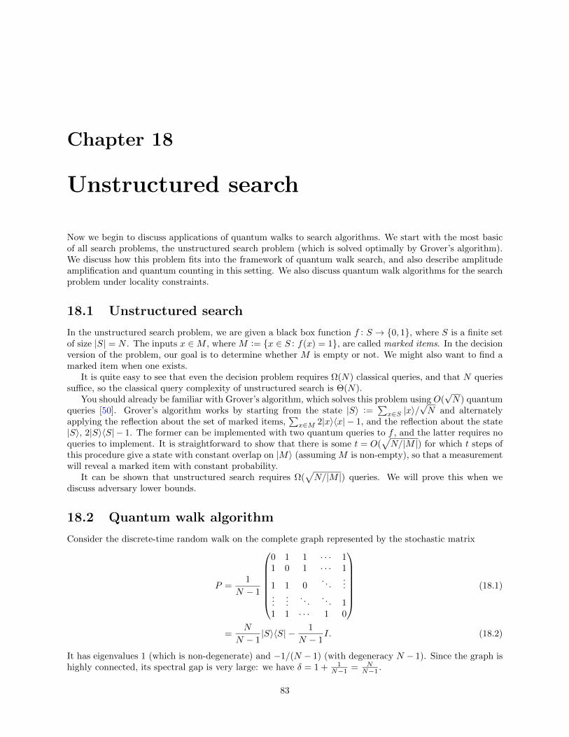
Chapter 18
Unstructured search
Now we begin to discuss applications of quantum walks to search algorithms. We start with the most basicof all search problems, the unstructured search problem (which is solved optimally by Grover’s algorithm).We discuss how this problem fits into the framework of quantum walk search, and also describe amplitudeamplification and quantum counting in this setting. We also discuss quantum walk algorithms for the searchproblem under locality constraints.
18.1 Unstructured search
In the unstructured search problem, we are given a black box function f : S → 0, 1, where S is a finite setof size |S| = N . The inputs x ∈M , where M := x ∈ S : f(x) = 1, are called marked items. In the decisionversion of the problem, our goal is to determine whether M is empty or not. We might also want to find amarked item when one exists.
It is quite easy to see that even the decision problem requires Ω(N) classical queries, and that N queriessuffice, so the classical query complexity of unstructured search is Θ(N).
You should already be familiar with Grover’s algorithm, which solves this problem using O(√N) quantum
queries [50]. Grover’s algorithm works by starting from the state |S〉 :=∑x∈S |x〉/
√N and alternately
applying the reflection about the set of marked items,∑x∈M 2|x〉〈x| − 1, and the reflection about the state
|S〉, 2|S〉〈S| − 1. The former can be implemented with two quantum queries to f , and the latter requires noqueries to implement. It is straightforward to show that there is some t = O(
√N/|M |) for which t steps of
this procedure give a state with constant overlap on |M〉 (assuming M is non-empty), so that a measurementwill reveal a marked item with constant probability.
It can be shown that unstructured search requires Ω(√N/|M |) queries. We will prove this when we
discuss adversary lower bounds.
18.2 Quantum walk algorithm
Consider the discrete-time random walk on the complete graph represented by the stochastic matrix
P =1
N − 1
0 1 1 · · · 11 0 1 · · · 1
1 1 0. . .
......
.... . .
. . . 11 1 · · · 1 0
(18.1)
=N
N − 1|S〉〈S| − 1
N − 1I. (18.2)
It has eigenvalues 1 (which is non-degenerate) and −1/(N − 1) (with degeneracy N − 1). Since the graph ishighly connected, its spectral gap is very large: we have δ = 1 + 1
N−1 = NN−1 .
83

84 Chapter 18. Unstructured search
This random walk gives rise to a very simple classical algorithm for unstructured search. In this algorithm,we start from a uniformly random item and repeatedly choose a new item uniformly at random from theother N−1 possibilities, stopping when we reach a marked item. The fraction of marked items is ε = |M |/N ,so the hitting time of this walk is
O
(1
δε
)=
(N − 1)N
N |M | = O(N/|M |) (18.3)
(this is only an upper bound on the hitting time, but in this case we know it is optimal). Of course, if wehave no a priori lower bound on |M | in the event that M is non-empty, the best we can say is that ε ≥ 1/N ,giving a running time O(N).
The corresponding quantum walk search algorithm has a hitting time of
O
(1√δε
)= O(
√N/|M |), (18.4)
corresponding to the running time of Grover’s algorithm. To see that this actually gives an algorithm usingO(√N/|M |) queries, we need to see that a step of the quantum walk can be performed using only O(1)
quantum queries. In the case where the first item is marked, the modified classical walk matrix is
P ′ =1
N − 1
N − 1 1 1 · · · 10 0 1 · · · 1
0 1 0. . .
......
.... . .
. . . 10 1 · · · 1 0
, (18.5)
so that the vectors |ψj〉 are |ψ1〉 = |1, 1〉 and |ψj〉 = |j, S \ j〉 =√
NN−1 |j, S〉 − 1√
N−1|j, j〉 for j = 2, . . . , N .
With a general marked set M , the projector onto the span of these states is
Π =∑j∈M|j, j〉〈j, j|+
∑j /∈M|j, S \ j〉〈j, S \ j|, (18.6)
so the operator 2Π− 1 acts as Grover diffusion over the neighbors when when the vertex is unmarked, andas a phase flip when the vertex is marked. (Note that since we start from the state |ψ〉 =
∑j /∈M |ψj〉, we
stay in the subspace of states span|j, k〉 : (j, k) ∈ E, and in particular have zero support on any state |j, j〉for j ∈ V , so 2Π − 1 acts as −1 when the first register holds a marked vertex.) Each such step can beimplemented using two queries of the black box, one to compute whether we are at a marked vertex andone to uncompute that information; the subsequent swap operation requires no queries. Thus the querycomplexity is indeed O(
√N/|M |).
This algorithm is not exactly the same as Grover’s; for example, it works in the Hilbert space CN ⊗CNinstead of CN . Nevertheless, it is clearly closely related. In particular, notice that in Grover’s algorithm,the unitary operation 2|S〉〈S| − 1 can be viewed as a kind of discrete-time quantum walk on the completegraph, where in this particular case no coin is necessary to define the walk.
The algorithm we have described so far only solves the decision version of unstructured search. To findmarked item, we could use bisection, but this would introduce a logarithmic overhead. In fact, it can beshown that the final state of the quantum walk algorithm actually encodes a marked item when one exists.
18.3 Amplitude amplification and quantum counting
We briefly mention some other concepts related to unstructured search that provide useful tools for quantumalgorithms in general. These ideas are typically presented in the context of Grover’s algorithm; here wedescribe them in the framework of quantum walk search. This is slightly less space efficient, but the essentialideas are the same.

18.4. Search on graphs 85
Amplitude amplification is a general method for boosting the success probability of a (classical or quan-tum) subroutine [23]. It can be implemented by quantum walk search as follows. Suppose we have aprocedure that produces a correct answer with probability p (i.e., with an amplitude of magnitude
√p if
we view it as a quantum process). From this procedure we can define a two-state Markov chain that, ateach step, moves from the state where the answer is not known to the state where the answer is known withprobability p, and then remains there. This walk has the transition matrix
P ′ =
(1− p 0p 1
),
so PM = 1− p, giving a quantum hitting time of O(1/√
1− ‖PM‖) = O(1/√p).
For some applications, it may be desirable to estimate the value of p. Quantizing the above two-state
Markov chain gives eigenvalues in the non-marked subspace of e±i arccos(1−p) = e±i√
2p+O(p3/2). By applyingphase estimation, we can determine
√p approximately. Recall that phase estimation gives an estimate with
precision µ using O(1/µ) applications of the given unitary [34] (assuming we cannot apply high powers of theunitary any more efficiently than simply applying it repeatedly). An estimate of
√p with precision µ gives
an estimate of p with precision µ√p (since (
√p+O(µ))2 = p+O(µ
√p)), so we can produce an estimate of
p with precision ν in O(√p/ν) steps.
In particular, if the Markov chain is a search of the complete graph as described in the previous section,with |M | marked sites out of N , then p = |M |/N , and this allows us to count the number of marked items.We obtain an estimate of |M |/N with precision ν in O(
√|M |/N/ν) steps. If we want a multiplicative
approximation of |M | with precision ρ, this means we need O(√N/|M |/ρ) steps.
Note that for exact counting, no speedup is possible in general. If |M | = Θ(N) then we need to estimatep within precision O(1/N) to uniquely determine |M |, but then the running time of the above procedure isO(N). In fact, it can be shown that exact counting requires Ω(N) queries [16].
18.4 Search on graphs
We can also consider a variant of unstructured search with additional locality constraints. Suppose we viewthe items in S as the vertices of a graph G = (S,E), and we require the algorithm to be local with respectto the graph. More concretely, we require the algorithm to alternate between queries and unitary operationsU constrained to satisfy U |j, ψ〉 =
∑k∈j∪∂(j) αk|k, φk〉 for any j ∈ S (where the second register represents
possible ancillary space, and recall that ∂(j) denotes the set of neighbors of j in G) [2].
Since we have only added new restrictions that an algorithm must obey, the Ω(√N) lower bound from
the non-local version of the problem still applies. However, it is immediately clear that this bound cannotalways be achieved. For example, if the graph is a cycle of N vertices, then simply propagating from onevertex of the cycle to an opposing vertex takes time Ω(N). So we would like to know, for example, how farfrom complete the graph can be such that we can still perform the search in O(
√N) steps.
First, note that any expander graph (a graph with degree upper bounded by a constant and secondlargest eigenvalue bounded away from 1 by a constant) can be searched in time O(
√N). Such graphs have
δ = Ω(1), and since ε ≥ 1/N when there are marked items, the quantum hitting time is O(1/√δε) = O(
√N)
(whereas the classical hitting time is O(1/δε) = O(N)).
There are also many cases in which a quantum search can be performed in time O(√N) even though the
eigenvalue gap of P is non-constant [89, 31, 12]. For example, consider the n-dimensional hypercube (withN = 2n vertices). Recall that since the adjacency matrix acts independently as σx on each coordinate, theeigenvalues are equally spaced, and the gap of P is 2/n. Thus the general bound in terms of the eigenvaluesof P shows that the classical hitting time is O(nN) = O(N logN). In fact, this bound is loose; the hittingtime is actually O(N), which can be seen by directly computing ‖PM‖ with one marked vertex. So there isa local quantum algorithm that runs in the square root of this time, namely O(
√N).
Perhaps the most interesting example is the d-dimensional square lattice with N sites (i.e., with linearsize N1/d). This case can be viewed as having N items distributed on a grid in d-dimensional space. Forsimplicity, suppose we have periodic boundary conditions; then the eigenstates of the adjacency matrix are

86 Chapter 18. Unstructured search
given by
|k〉 :=1√N
∑x
e2πik·x/N1/d |x〉 (18.7)
where k is a d-component vector of integers from 0 to N1/d − 1. The corresponding eigenvalues are
2
d∑j=1
cos2πkjN1/d
. (18.8)
Normalizing to obtain a stochastic matrix, we simply divide these eigenvalues by 2d. The 1 eigenvector hask = (0, 0, . . . , 0), and the second largest eigenvalue comes from (e.g.) k = (1, 0, . . . , 0), with an eigenvalue
1
d
(d− 1 + cos
2π
N1/d
)≈ 1− 1
2d
(2π
N1/d
)2
. (18.9)
Thus the gap of the walk matrix P is about 2π2
dN2/d = O(N−2/d). This is another case in which the bound
on the classical hitting time in terms of eigenvalues of P is too loose (it gives only O(N1+2/d)), and insteadwe must directly estimate the gap of PM . One can show that the classical hitting time is O(N2) in d = 1,O(N logN) in d = 2, and O(N) for any d ≥ 3. Thus there is a local quantum walk search algorithm thatsaturates the lower bound for any d ≥ 3, and one that runs in time time O(
√N logN) for d = 2. We already
argued that there could be no speedup for d = 1, and indeed we see that the quantum hitting time in thiscase is O(N).

Chapter 19
Quantum walk search
In this lecture we will discuss the algorithm that cemented the importance of quantum walk as a tool forquantum query algorithms: Ambainis’s algorithm for the element distinctness problem [11]. The key newconceptual idea of this algorithm is to consider walks that store information obtained from many queries ateach vertex, but that do not require many queries to update this information for an adjacent vertex. Thisidea leads to a general, powerful framework for quantum walk search [70, 84].
19.1 Element distinctness
In the element distinctness problem, we are given a black-box function f : 1, . . . , n → S, where S issome finite set. The goal is to determine whether there are two distinct inputs x, y ∈ 1, . . . , n such thatf(x) = f(y).
It is clear that a classical algorithm must make Ω(n) queries to solve the problem, since deciding whetherthere is such a pair is at least as hard as unstructured search (suppose we give the additional promise that ifthere is a pair, it will be with x = 1 for which f(1) = 1; then we must search for a y ∈ 2, . . . , n for whichf(y) = 1). By the same argument, there is a quantum lower bound for element distinctness of Ω(
√n).
There is a simple quantum algorithm that uses Grover’s algorithm recursively to improve upon the trivialrunning time of O(n) [26]. To see how this algorithm works, first consider the following subroutine. Queryf in ` randomly chosen places, and check whether one of these ` places belongs to a pair of inputs that mapto the same value by performing a Grover search on the remaining n − ` inputs. The initial setup takes `queries, and the Grover search takes O(
√n− `) = O(
√n) queries, for a total of `+O(
√n). This subroutine
fails most of the time, since it is likely that the random choice of ` inputs will be unlucky, but it succeeds withprobability at least `/n. To boost the success probability, we can use amplitude amplification, which takesO(√n/`) steps to boost the success probability to a constant. Overall, we can obtain success probability
Ω(1) using
(`+√n)√n/` =
√n`+ n/
√` (19.1)
queries. To optimize the query complexity, we set the two terms to be equal, giving ` =√n and hence a
query complexity of O(n3/4). (Note that an analysis of the running time of this algorithm would includeextra logarithmic factors, since the inner use of Grover’s algorithm must check whether an element against` queried function values, which can be done in time O(log `) provided S is ordered and we initially sort thequeried values.)
So far, we have a quantum upper bound of O(n3/4), and a quantum lower bound of Ω(n1/2). It turns outthat both of these can be improved. On the lower bound side, Aaronson and Shi proved an Ω(n1/3) lowerbound for the closely-related collision problem, in which the goal is to distinguish one-to-one from two-to-one functions [3]. This implies an Ω(n2/3) lower bound for element distinctness by the following reduction.Suppose we randomly choose
√n inputs of the collision problem function and run the element distinctness
algorithm on them. If the function is two-to-one, then there is some pair of elements in this set mapping tothe same value with high probability (by the birthday problem), which the element distinctness algorithm
87

88 Chapter 19. Quantum walk search
will detect. Hence a k-query element distinctness algorithm implies an O(√k)-query collision algorithm; or
equivalently, a k-query collision lower bound implies an Ω(k2) element distinctness lower bound.Now the question remains, can we close the gap between the O(n3/4) upper bound and this Ω(n2/3) lower
bound? Ambainis’s quantum walk algorithm does exactly this.
19.2 Quantum walk algorithm
The idea of Ambainis’s algorithm is to quantize a walk on the Johnson graph J(n,m), where m is chosenappropriately. This graph has
(nm
)vertices corresponding to subsets of 1, 2, . . . , n of size m, and two
vertices are connected by an edge if the subsets differ in exactly one element.To simplify the analysis slightly, we will use a different graph, the Hamming graph H(n,m). The vertices
of this graph are the m-tuples of values from 1, 2, . . . , n (so there are nm vertices). Two vertices areconnected by an edge if they differ in exactly one coordinate. There are two main differences between theJohnson and Hamming graphs: the Hamming graph allows for repeated elements, and the order of elementsis significant. Neither of these differences significantly affects the performance of the algorithm.
At each vertex, we store the values of the function at the corresponding inputs. In other words, thevertex (x1, x2, . . . , xm) ∈ 1, 2, . . . , nm is represented by the state
|x1, x2, . . . , xm, f(x1), f(x2), . . . , f(xm)〉. (19.2)
To prepare such states, we must query the black-box function. In particular, to prepare an initial superpo-sition over vertices of this graph takes m queries. However, we can move from one vertex to an adjacentvertex using only two queries: to replace x by y in any particular coordinate, we use one query to erase f(x)and another to compute f(y).
In this search problem, the marked vertices are those containing some x 6= y with f(x) = f(y). Noticethat, given the stored function values, we can check whether we are at a marked vertex with no additionalqueries. The total number of marked vertices (in the case where the elements are not all distinct) is at leastm(m− 1)(n− 2)m−2, so the fraction of marked vertices is
ε ≥ m(m− 1)(n− 2)m−2
nm. (19.3)
To analyze the walk, we also need the eigenvalues of the relevant Markov chain. The adjacency matrixof the Hamming graph H(n,m) is A =
∑mi=1(J − I)(i), where J denotes the n × n all 1s matrix, and
the superscript indicates that this matrix acts on the ith coordinate. The eigenvalues of J are n and0, so the eigenvalues of J − I are n − 1 and −1. Hence the largest eigenvalue of A is m(n − 1) (thedegree of any vertex of H(n,m)) and the second largest eigenvalue is (m − 1)(n − 1) − 1 = m(n − 1) − n.Normalizing by the degree, we see that the second largest eigenvalue of the stochastic matrix A/m(n− 1) is(m(n− 1)− n)/m(n− 1) = 1− n/m(n− 1). In other words, the spectral gap is
δ =n
m(n− 1). (19.4)
Finally, how many queries does this algorithm use? Taking into account the initial m queries used toprepare the starting state and the 2 queries per step of the walk, we have a total number of queries
m+ 2 ·O(
1√δε
)= m+O
(√m(n− 1)
n
√nm
m(m− 1)(n− 2)m−2
)(19.5)
= m+O
(n√m
). (19.6)
Again we can set the two terms equal to optimize the performance. We have m3/2 = O(n), so we shouldtake m = Θ(n2/3). Then the total number of queries is O(n2/3), which matches the lower bound, and henceis optimal.
Note that for the classical random walk search algorithm that we have quantized, the correspondingquery complexity is m+O(n2/m), which is optimized by m = n. This gives no improvement over queryingevery input, as we knew must be the case.

19.3. Quantum walk search algorithms with auxiliary data 89
19.3 Quantum walk search algorithms with auxiliary data
Algorithms based on similar ideas turn out to be useful for a wide variety of problems, including decidingwhether a graph contains a triangle (or various other related graph properties), checking matrix multiplica-tion, and testing whether a group is abelian. In general, as in the element distinctness case, we may need tostore some data at each vertex, and we need to take into account the operations on this data when analyzingthe walk.
Suppose we have a setup cost S, a cost U to update the state after one step of the walk, and a cost C tocheck whether a vertex is marked. For example, in Ambainis’s algorithm for element distinctness, we had
S = m to query m positions (19.7)
U = 2 to remove one of the items and add another (19.8)
C = 0 since the function values for the subset are stored. (19.9)
In general, there is an algorithm to solve such a problem with total cost
S +1√δε
(U + C). (19.10)
It turns out that for some problems, when the checking cost C is much larger than the update cost U ,it is advantageous to take many steps of the walk on the unmarked graph before performing a phase flip onthe marked sites. This is how Ambainis’s algorithm originally worked, though for element distinctness it isnot actually necessary. Using this idea, one can give a general quantum walk search algorithm with totalcost [70]
S +1√ε
(1√δU + C
). (19.11)
In fact, it is also possible to modify the general algorithm so that it finds a marked item when one exists.

90 Chapter 19. Quantum walk search

Part IV
Quantum query complexity
91


Chapter 20
Query complexity and the polynomialmethod
So far, we have discussed several different kinds of quantum algorithms. In the next few chapters, we discussways of establishing limitations on the power of quantum algorithms [57]. After reviewing the model ofquantum query complexity, this chapter presents the polynomial method, an approach that relates quantumquery algorithms to properties of polynomials.
20.1 Quantum query complexity
Many of the algorithms we have covered work in the setting of query complexity, where the input for aproblem is provided by a black box. This setting is convenient since the black box provides a handle forproving lower bounds: we can often show that many queries are required to compute some given functionof the black-box input. In contrast, it is notoriously difficult to prove lower bounds on the complexity ofcomputing some function of explicit input data.
We briefly formalize the model of query complexity. Consider the task of computing a function f : S → T ,where S ⊆ Σn is a set of strings over some input alphabet Σ. If S = Σn then we say f is total ; otherwise wesay it is partial. The input string x ∈ S is provided to us by a black box that computes xi for any desiredi ∈ 1, . . . , n. A query algorithm begins from a state that does not depend on the oracle string x. It thenalternates between queries to the black box and other, non-query operations. Our goal is to compute f(x)using as few queries to the black box as possible.
Of course, the minimum number of queries (which we call the query complexity of f) depends on thekind of computation we allow. There are at least three natural models:
• D(f) denotes the deterministic query complexity, where the algorithm is classical and must alwayswork correctly.
• Rε denotes the randomized query complexity with error probability at most ε. Note that this it does notdepend strongly on ε since we can boost the success probability by repeating the computation severaltimes and taking a majority vote. Therefore Rε(f) = Θ(R1/3(f)) for any constant ε, so sometimes wesimply write R(f).
• Qε denotes the quantum query complexity, again with error probability at most ε. Similarly to therandomized case, Qε(f) = Θ(Q1/3(f)) for any constant ε, so sometimes we simply write Q(f).
We know that D(or) = n and R(or) = Θ(n). Grover’s algorithm shows that Q(or) = O(√n). In this
lecture we will use the polynomial method to show (among other things) that Q(or) = Ω(√n), a tight lower
bound.
93

94 Chapter 20. Query complexity and the polynomial method
20.2 Quantum queries
A quantum query algorithm begins from x-independent state |ψ〉 and applies a sequence of unitary operationsU1, . . . , Ut interspersed with queries Ox, resulting in the state
|ψtx〉 := UtOx . . . U2OxU1Ox|ψ〉. (20.1)
To make this precise, we need to specify the action of the oracle Ox.
For simplicity, we will mostly consider the case where the input is a bit string, i.e., Σ = 0, 1. Perhapsthe most natural oracle model is the bit flip oracle Ox, which acts as
Ox|i, b〉 = |i, b⊕ xi〉 for i ∈ 1, . . . , n, b ∈ 0, 1. (20.2)
This is simply the linear extension of the natural reversible oracle mapping (i, b) 7→ (i, b⊕ xi), which can beperformed efficiently given the ability to efficiently compute i 7→ xi. Note that the algorithm may involvestates in a larger Hilbert space; implicitly, the oracle acts as the identity on any ancillary registers.
It is often convenient to instead consider the phase oracle, which is obtained by conjugating the bit-fliporacle by Hadamard gates: by the well-known phase kickback trick, Ox = (I ⊗H)Ox(I ⊗H) satisfies
Ox|i, b〉 = (−1)bxi |i, b〉 for i ∈ 1, . . . , n, b ∈ 0, 1. (20.3)
Note that this is slightly wasteful since Ox|i, 0〉 = |i, 0〉 for all i; we could equivalently consider a phase oracleO′x defined by O′x|0〉 = |0〉 and O′x|i〉 = (−1)xi |i〉 for all i ∈ 1, . . . , n. However, it is essential to include theability to not query the oracle by giving the oracle some eigenstate of known eigenvalue, independent of x.If we could only perform the phase flip |i〉 7→ (−1)xi |i〉 for i ∈ 1, . . . , n, then we could not tell a string xfrom its bitwise complement x.
These constructions can easily be generalized to the case of a d-ary input alphabet, say Σ = Zd (identifyinginput symbols with integers modulo d). Then for b ∈ Σ, we can define an oracle Ox by
Ox|i, b〉 = |i, b+ xi〉 for i ∈ 1, . . . , n, b ∈ Zd. (20.4)
Taking the Fourier transform of the second register gives a phase oracle Ox = (I⊗FZd)Ox(I⊗F †Zd) satisfying
Ox|i, b〉 = ωbxid |i, b〉 for i ∈ 1, . . . , n, b ∈ Zd (20.5)
where ωd := e2πi/d.
20.3 Quantum algorithms and polynomials
The following shows a basic connection between quantum algorithms and polynomials [16].
Lemma 20.1. The acceptance probability of a t-query quantum algorithm for a problem with black-box inputx ∈ 0, 1n is a polynomial in x1, . . . , xn of degree at most 2t.
Proof. We claim that the amplitude of any basis state is a polynomial of degree at most t, so that theprobability of any basis state (and hence the probability of success) is a polynomial of degree at most 2t.
The proof is by induction on t. If an algorithm makes no queries to the input, then its success probabilityis independent of the input, so it is a constant, a polynomial of degree 0.
For the induction step, a query maps
|i, b〉 Ox7→ (−1)bxi |i, b〉 (20.6)
= (1− 2bxi)|i, b〉, (20.7)
so it increases the degree of each amplitude by at most 1.

20.4. Symmetrization 95
Consider a Boolean function f : 0, 1n → 0, 1. We say a polynomial p ∈ R[x1, . . . , xn] represents f ifp(x) = f(x) for all x ∈ 0, 1n. Letting deg(f) denote the smallest degree of any polynomial representing f ,we have Q0(f) ≥ deg(f)/2.
To handle bounded-error algorithms, we introduce the concept of approximate degree. We say a polyno-mial p ε-represents f if |p(x) − f(x)| ≤ ε for all x ∈ 0, 1n. Then the ε-approximate degree of f , denoted
degε(f), is the smallest degree of any polynomial that ε-represents f . Clearly, Qε(f) ≥ degε(f)/2. Sincebounded-error query complexity does not depend strongly on the particular error probability ε, we can define,
say, deg(f) := deg1/3(f).Now to lower bound the quantum query complexity of a Boolean function, it suffices to lower bound its
approximate degree.
20.4 Symmetrization
While polynomials are well-understood objects, the acceptance probability is a multivariate polynomial, soit can be rather complicated. Since x2 = x for x ∈ 0, 1, we can restrict our attention to multilinearpolynomials, but it is still somewhat difficult to deal with such polynomials directly. Fortunately, for manyfunctions it suffices to consider a related univariate polynomial obtained by symmetrization.
For a string x ∈ 0, 1n, let |x| denote the Hamming weight of x, the number of 1s in x.
Lemma 20.2. Given any n-variate multilinear polynomial p, let P (k) := E|x|=k[p(x)]. Then P is a polyno-mial with deg(P ) ≤ deg(p).
Proof. Since p is multilinear, it can be written as a sum of monomials, i.e., as
p(x) =∑
S⊆1,...,ncS∏i∈S
xi (20.8)
for some coefficients cS . Then we have
P (k) =∑
S⊆1,...,ncS E|x|=k
[∏i∈S
xi
](20.9)
and it suffices to compute the expectation of each monomial. We find
E|x|=k
[∏i∈S
xi
]= Pr|x|=k
[∀ i ∈ S, xi = 1] (20.10)
=
(n−|S|k−|S|
)(nk
) (20.11)
=(n− |S|)! k! (n− k)!
(k − |S|)! (n− k)!n!(20.12)
=(n− |S|)!
n!k(k − 1) · · · (k − |S|+ 1) (20.13)
which is a polynomial in k of degree |S|. Since cS = 0 whenever |S| > deg(p), we see that deg(P ) ≤deg(p).
Thus the polynomial method is a particularly natural approach for symmetric functions, those that onlydepend on the Hamming weight of the input.
20.5 Parity
Let parity : 0, 1n → 0, 1 denote the symmetric function parity(x) = x1⊕· · ·⊕xn. Recall that Deutsch’sproblem, which is the problem of computing the parity of 2 bits, can be solved exactly with only one quantum
96 Chapter 20. Query complexity and the polynomial method
query. Applying this algorithm to a pair of bits at a time and then taking the parity of the results, we seethat Q0(parity) ≤ n/2.
What can we say about lower bounds for computing parity? Symmetrizing parity gives the functionP : 0, 1, . . . , n → R defined by
P (k) =
0 if k is even
1 if k is odd.(20.14)
Since P changes direction n times, deg(P ) ≥ n, so we see that Q0(parity) ≥ n/2. Thus Deutsch’s algorithmis tight among zero-error algorithms.
What about bounded-error algorithms? To understand this, we would like to lower bound the approxi-mate degree of parity. If |p(x)− f(x)| ≤ ε for all x ∈ 0, 1n, then
|P (k)− F (k)| =∣∣∣∣ E|x|=k
(p(x)− f(x))
∣∣∣∣ ≤ ε (20.15)
for all k ∈ 0, 1, . . . , n, where P is the symmetrization of p and F is the symmetrization of f . Thus, amultilinear polynomial p that ε-approximates parity implies a univariate polynomial P satisfying P (k) ≤ εfor k even and P (k) ≥ 1 − ε for k odd. For any ε < 1/2, this function still changes direction n times, so in
fact we have degε(f) ≥ n, and hence Qε(parity) ≥ n/2.This shows that the strategy for computing parity using Deutsch’s algorithm is optimal, even among
bounded-error algorithms. This is an example of a problem for which a quantum computer cannot get asignificant speedup—here the speedup is only by factor of 2. In fact, we need at least n/2 queries to succeedwith any bounded error, even with very small advantage (e.g., even if we only want to be correct withprobability 1
2 + 10−100). In contrast, while the adversary method can prove an Ω(n) lower bound for parity,the constant factor that it establishes is error-dependent.
Note that this also shows we need Ω(n) queries to exactly count the number of marked items in anunstructured search problem, since exactly determining the number of 1s would in particular determinewhether the number of 1s is odd or even.
20.6 Unstructured search
Next we will see how the polynomial method can be used to prove the Ω(√n) lower bound for computing
the logical or of n bits. Symmetrizing or gives a function F (k) with F (0) = 0 and F (1) = 1. We also haveF (k) = 1 for all k > 1, but we will not actually need to use this. This function is monotonic, so we cannot
use the same simple argument we applied to parity. Nevertheless, we can prove that deg(or) = Ω(√n) using
the following basic fact about polynomials, due to Markov.
Lemma 20.3. Let P : R→ R be a polynomial. Then
maxx∈[0,n]
dP (x)
dx≤ deg(P )2
n
(maxx∈[0,n]
P (x)− minx∈[0,n]
P (x)
). (20.16)
In other words, if we leth := max
x∈[0,n]P (x)− min
x∈[0,n]P (x) (20.17)
denote the “height” of P in the range [0, n], and
d := maxx∈[0,n]
dP (x)
dx(20.18)
denote the largest derivative of P in that range, then we have deg(P ) ≥√nd/h.
Now let P be a polynomial that ε-approximates or. Since P (0) ≤ ε and P (1) ≥ 1− ε, P must increaseby at least 1− 2ε in going from k = 0 to k = 1, so d ≥ 1− 2ε.
We have no particular bound on h, since we have no control over the value of P at non-integer points; thefunction could become arbitrarily large or small. However, since P (k) ∈ [0, 1] for k ∈ 0, 1, . . . , n, a large

20.6. Unstructured search 97
value of h implies a large value of d, since P must change fast enough to start from and return to values inthe range [0, 1]. In particular, P must change by at least (h− 1)/2 over a range of k of width at most 1/2,so we have d ≥ h− 1. Therefore,
deg(P ) ≥√nmax1− 2ε, h− 1
h(20.19)
= Ω(√n). (20.20)
It follows that Q(or) = Ω(√n).
Note that the same argument applies for a function that takes the value 0 whenever |x| = w and the value1 whenever |x| = w + 1, for any w; in particular, it applies to any non-constant symmetric function. (Ofcourse, we can do better for some symmetric functions, such as parity and also majority, among others.)

98 Chapter 20. Query complexity and the polynomial method
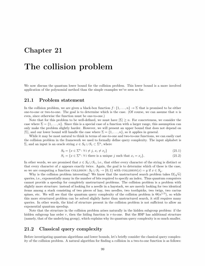
Chapter 21
The collision problem
We now discuss the quantum lower bound for the collision problem. This lower bound is a more involvedapplication of the polynomial method than the simple examples we’ve seen so far.
21.1 Problem statement
In the collision problem, we are given a black-box function f : 1, . . . , n → Σ that is promised to be eitherone-to-one or two-to-one. The goal is to determine which is the case. (Of course, we can assume that n iseven, since otherwise the function must be one-to-one.)
Note that for this problem to be well-defined, we must have |Σ| ≥ n. For concreteness, we consider thecase where Σ = 1, . . . , n. Since this is a special case of a function with a larger range, this assumption canonly make the problem slightly harder. However, we will present an upper bound that does not depend on|Σ|, and our lower bound will handle the case where Σ = 1, . . . , n, so it applies in general.
While it may be most natural to think in terms of one-to-one and two-to-one functions, we can easily castthe collision problem in the framework we used to formally define query complexity. The input alphabet isΣ, and an input is an oracle string x ∈ S0 ∪ S1 ⊂ Σn, where
S0 = x ∈ Σn : ∀ i 6= j, xi 6= xj (21.1)
S1 = x ∈ Σn : ∀ i there is a unique j such that xi = xj. (21.2)
In other words, we are promised that x ∈ S0 ∪ S1, i.e., that either every character of the string is distinct orthat every character of x appears exactly twice. Again, the goal is to determine which of these is the case,so we are computing a function collision : S0 ∪ S1 → 0, 1 with collision(x) = y if x ∈ Sy.
Why is the collision problem interesting? We know that the unstructured search problem takes Ω(√n)
queries, i.e., exponentially many in the number of bits required to specify an index. Thus quantum computerscannot provide a speedup for completely unstructured problems. The collision problem is a problem withslightly more structure: instead of looking for a needle in a haystack, we are merely looking for two identicalitems among a stack consisting of two pieces of hay, two needles, two toothpicks, two twigs, two cactusspines, etc. We will see that the quantum query complexity of the collision problem is Θ(n1/3), so whilethis more structured problem can be solved slightly faster than unstructured search, it still requires manyqueries. In other words, the kind of structure present in the collision problem is not sufficient to allow anexponential quantum speedup.
Note that the structure in the collision problem arises naturally in the hidden subgroup problem: if thehidden subgroup has order r, then the hiding function is r-to-one. But the HSP has additional structure(namely, that of the underlying group), which explains why its quantum query complexity is so much smaller.
21.2 Classical query complexity
Before investigating quantum algorithms and lower bounds, let’s briefly consider the classical query complex-ity of the collision problem. A natural algorithm for finding a collision in a two-to-one function is as follows:
99

100 Chapter 21. The collision problem
query random indices until we observe a collision. For two independently random indices i, j ∈ 1, . . . , n,we have Pr(xi = xj) = 1
n−1 . If we query m indices in this way, there are(m2
)pairs, so the expected number
of collisions seen is(m2
)/(n− 1). With m =
√n this is Ω(1), so we expect to see a collision. Indeed, a second
moment argument shows that this happens with constant probability.In fact, this algorithm is optimal. Until we see a collision, there is no better strategy than to query
randomly. By the union bound, the probability of seeing a collision after making m queries is at most(m2
)/(n− 1) = O(m2/n), so m = Ω(
√n).
21.3 Quantum algorithm
Now let’s consider quantum algorithms for the collision problem. One simple approach is a trivial applicationof Grover’s algorithm: first query x1, and then search over x2, x3, . . . , xn for x1. This approach uses O(
√n)
queries, so it is no better than the above classical algorithm, although it achieves the same running time ina very different way.
However, we can improve the performance by combining this approach with the main idea of the optimalclassical algorithm. The approach is to query m distinct indices (it doesn’t matter how we choose them) andcheck for a collision. If we find a collision then we are done; otherwise, we can search the remaining n−mcharacters for one of the m values we have seen. Overall, this approach takes time m + O(
√(n−m)/m).
This is minimized by taking m = Θ(n1/3), showing that Q(collision) = O(n1/3) [24].This is similar to an algorithm for element distinctness that we saw previously. The difference is that in
element distinctness, we could have a unique collision, so a single run of the basic algorithm only succeedswith small probability; we address this by performing amplitude amplification, at the cost of a longer runningtime. Recall that the resulting algorithm for element distinctness took time O(n3/4), which turned out tobe suboptimal. In contrast, the above algorithm for the collision problem turns out to be optimal.
As a side remark, note that this algorithm uses a lot of space, since we need to store the m = n1/3 itemsqueried initially. It is an open problem to understand the quantum query complexity of the collision problemwith restricted space (i.e., to find a time-space tradeoff).
21.4 Toward a quantum lower bound
How can we prove a quantum lower bound for the collision problem?Note that the positive-weighted adversary method will not be sufficient. This is a consequence of the
so-called “property-testing barrier”: for a decision problem in which “yes” input strings differ from “no”input strings in an ε fraction of their characters, the best possible positive adversary lower bound goes like1/ε. For the collision problem, this means that the adversary method can at best prove a constant lowerbound. (There is now an explicit Ω(n1/3) lower bound for collision using the negative adversary method[18], although it is somewhat complicated.)
Thus our strategy will be to apply the polynomial method. To do this, we need to adapt the method tothe case of a non-binary input alphabet. To do this, we define variables δij for i, j ∈ 1, . . . , n, as follows:
δij :=
1 if xi = j
0 otherwise.(21.3)
Then we claim that acceptance probability of a t-query quantum algorithm is a multilinear polynomial inthe δij of degree at most 2t.
This can be proved along similar lines to the binary case. Suppose we use an addition modulo n query,where |i, j〉 7→ |i, j + xi〉. Then we have
|i, j + xi〉 =∑k
δik|i, j + k〉 (21.4)
=∑`
δi,`−j |i, `〉, (21.5)

21.5. Constructing the functions 101
so the degree of each amplitude can increase by at most 1 when we make a query.
Next we would like to obtain a simpler polynomial. We cannot directly symmetrize over the variablesδij, as this would destroy too much of the structure of the problem.
The original idea leading to a nontrivial collision lower bound, due to Aaronson, was to express theacceptance probability as a bivariate polynomial in n and r, where the function is r-to-one. The maindifficulty with this approach is that we need to have r | n in order for such inputs to make sense (so thatwe can at least say that the acceptance probability of a quantum algorithm is defined, and hence a givenapproximating polynomial is bounded between 0 and 1). This approach originally gave a lower bound Ω(n1/5)[1]. Subsequently, Shi improved this to give the optimal result of Ω(n1/3) [90].
21.5 Constructing the functions
In this lecture we will describe a later argument due to Kutin [65] that seems to be simplest known approachto lower bounding the collision problem, yet that gives a tight lower bound, and even covers the case wherethe range is 1, . . . , n. We will follow Kutin’s presentation closely, with only some slight changes of notation.
The basic idea of Kutin’s proof is to consider functions that are a-to-one on part of the domain andb-to-one on the rest of the domain. Let us say that a triple (m, a, b) is valid if m ∈ 0, 1, . . . , n, a | m, andb | n−m. Then we define an input xm,a,b as
xm,a,bi =
di/ae if 1 ≤ i ≤ mn− b(n− i)/bc if m < i ≤ n. (21.6)
Given such an input, we can obtain a family of inputs by permuting the input alphabet and the charactersof the string arbitrarily. Specifically, for any permutations στ of 1, . . . , n, we define an input xστ with
xστi := τ(xm,a,bσ(i) ). This induces corresponding binary variables δστij with δστij = 1 iff xστi = j.
Now we claim that the acceptance probability of a quantum algorithm presented with such an input is apolynomial in m, a, b.
Lemma 21.1. Let p(δij) be a polynomial in the δij. For any valid triple (m, a, b), let
P (m, a, b) := Eσ,τ
[p(δστij )]. (21.7)
Then P is a polynomial in m, a, b with deg(P ) ≤ deg(p).
Proof. Any polynomial p can be expanded as a sum of monomials of the form
IS(δij) :=
n∏j=1
∏i∈Sj
δij (21.8)
where S1, . . . , Sn are disjoint subsets of 1, . . . , n. This monomial is 1 if all the indices i ∈ Sj satisfy xi = j,and 0 otherwise. Its degree is s :=
∑j |Sj |. It suffices to handle the case where p is any particular monomial.
For any input xστ , we can identify the subset of function values in the range of the a-to-one part of thefunction and the b-to-one part of the function. Given U ⊆ 1, . . . , n, let X denote the event that all functionvalues in U belong to the a-to-one part and all function values not in U belong to the b-to-one part (moreformally, that τ(j) ∈ U for all j ∈ 1, . . . , ma with Sj 6= ∅ and τ(j) /∈ U for all j ∈ n, n−1, . . . , n− n−m
b +1with Sj 6= ∅). We collect together the inputs corresponding to a particular event X. Then we have
P (m, a, b) =∑
U⊆1,...,nPrτ
[X] Eσ,τ
[IS(δστij ) | X] (21.9)
=∑
U⊆1,...,nPrτ
[X] Prσ,τ
[∀ j, ∀ i ∈ Sj , δστij = 1 | X]. (21.10)

102 Chapter 21. The collision problem
Let u := |U |, and let t denote the number of values of j with |Sj | 6= 0. Then we have
Prτ
[X] =ma (ma − 1) · · · (ma − u+ 1) · (n−mb )(n−mb − 1) · · · (n−mb − (t− u) + 1) · (n− t)!
n!(21.11)
=(ma )u(n−mb )t−u
(n)t(21.12)
where
(n)k :=n!
(n− k)!= n(n− 1) · · · (n− k + 1). (21.13)
Here the numerator of (21.11) has three contributions: the number of ways to permute the u function valuesin the a-to-one part is (ma )u, the number of ways to permute the t−u function values in the b-to-one part is(n−mb )t−u, and the number of ways to permute the n− t remaining function values is (n− t)!. Note that thisexpression is a rational function in m, a, b whose numerator has degree t and whose denominator is aubt−u.
Now consider the latter term of (21.10). Given that X occurs, Prτ [∀ j, ∀ i ∈ Sj , δστij = 1] is independentof σ, so suppose σ is any permutation such that X occurs. In other words, we only need to count consistentways of permuting the indices i. Observe that the number of ways to permute the indices i such that xi = jfor some j ∈ U is
a(a− 1) · · · (a− |Sj |+ 1) = (a)|Sj |. (21.14)
Similarly, the number of ways to permute the indices i such that xi = j for some j /∈ U is (b)|Sj |. In addition,we can permute the remaining n− s indices however we like. Thus we have
Prσ,τ
[∀ j, ∀ i ∈ Sj , δστij = 1 | X] =(n− s)!∏j∈U (a)|Sj
∏j /∈U (b)|Sj |
n!(21.15)
=
∏j∈U (a)|Sj |
∏j /∈U (b)|Sj |
(n)s. (21.16)
This expression is a polynomial in a, b of degree s. Also, it is divisible by au and bt−u. Thus P (m, a, b) is apolynomial in m, a, b of degree t+ s− u− (t− u) = s.
21.6 Finishing the proof
To prove the lower bound, we will use the following fact about real polynomials. (Note that this fact is alsouseful elsewhere, e.g., in proving a tight lower bound for general threshold functions.)
Lemma 21.2 (Paturi). Let f ∈ R[x], let a, b ∈ Z with a < b, and let ξ ∈ [a, b]. If there are constants c, dsuch that• |f(i)| ≤ c for all integers i ∈ [a, b]
• |f(bξc)− f(ξ)| ≥ d,then deg(f) = Ω(
√(ξ − a+ 1)(b− ξ + 1)).
Regardless of ξ, Paturi’s lemma always shows that the degree is Ω(√b− a). If ξ is near the middle of
the range then it does much better, showing that the degree is Ω(b− a). Also note that by continuity, it issufficient for f to differ by a constant amount between two consecutive integers.
Now we are ready to prove that the quantum query complexity of the collision problem is Ω(n1/3). Letp(δij) be the acceptance probability of a t-query quantum algorithm that solves the collision problem witherror probability at most 1/3, and let P (m, a, b) be as above. We know that t ≥ deg(P )/2. Furthermore, weknow that P has the following properties:
• 0 ≤ P (m, 1, 1) ≤ 1/3
• 2/3 ≤ P (m, 2, 2) ≤ 1
• 0 ≤ P (m, a, b) ≤ 1 for any valid triple (m, a, b).

21.6. Finishing the proof 103
Now consider inputs that are roughly half one-to-one and half two-to-one. For concreteness, let m =2bn/4c. Since n − m is even (recall that n is always even by assumption since otherwise the problem istrivial), (m, 1, 2) is valid. We consider two cases, depending on whether the algorithm is more likely to callthis a yes or a no input. First suppose P (m, 1, 2) ≥ 1/2.
Let r be the smallest integer such that |P (m, 1, r)| ≥ 2. First we consider P (m, 1, x) as a function of x.For all x ∈ 1, . . . , r − 1, we have −2 ≤ P (m, 1, x) ≤ 2. But we also know that |P (m, 1, 1)− P (m, 1, 2)| ≥12 − 1
3 = 16 . By Paturi’s lemma, this implies that deg(P ) = Ω(
√r).
On the other hand, consider the polynomial g(x) := P (n − rx, 1, r). When x ∈ Z such that rx ∈0, . . . , n, the triple (n− rx, 1, r) is valid, so we have 0 ≤ g(x) ≤ 1 for all integers x ∈ [0, bn/rc]. However,|g(n−mr )| = |P (n, 1, r)| ≥ 2, and
⌊n−mr
⌋is about halfway between 0 and bn/rc. Thus by Paturi’s lemma,
deg(P ) = Ω(n/r).Combining these results, we have deg(P ) = Ω(
√r + n/r). The weakest lower bound is obtained when
the two terms are equal, i.e., when r = Θ(n2/3); therefore deg(P ) = Ω(n1/3).It remains to consider the case where |P (m, 1, r)| < 1/2. But the same conclusion holds here by a very
similar argument. (Let r be the smallest even integer for which |P (m, r, 2)| ≥ 2; on the one hand, deg(P ) =Ω(√d) as before, but on the other hand, the polynomial h(x) := P (rx, r, 2) shows that deg(P ) = Ω(n/r).)
Overall, it follows that any quantum algorithm for solving the collision problem must use Ω(n1/3) queries.

104 Chapter 21. The collision problem

Chapter 22
The quantum adversary method
We now discuss a second approach to proving quantum query lower bounds, the quantum adversary method[10]. In fact, we’ll see later that the generalized version of the adversary method we consider here (allowingnegative weights [55]) turns out to be an upper bound on quantum query complexity, up to constant factors[79, 68].
22.1 Quantum adversaries
Motivation for the quantum adversary method comes from the following construction. Suppose the oracle isoperated by an adversarial party who holds a quantum state determining the oracle string, which is in somesuperposition
∑x∈S ax|x〉 over the possible oracles. To implement each query, the adversary performs the
“super-oracle”
O :=∑x∈S|x〉〈x| ⊗Ox. (22.1)
An algorithm does not have direct access to the oracle string, and hence can only perform unitary operationsthat act as the identity on the adversary’s superposition. After t steps, an algorithm maps the overall stateto
|ψt〉 := (I ⊗ Ut)O . . . (I ⊗ U2)O(I ⊗ U1)O
(∑x∈S
ax|x〉 ⊗ |ψ〉)
(22.2)
=∑x∈S
ax|x〉 ⊗ |ψtx〉. (22.3)
The main idea of the approach is that for the algorithm to learn x, this state must become very entangled.To measure the entanglement of the pure state |ψt〉, we can consider the reduced density matrix of the oracle,
ρt :=∑x,y∈S
a∗xay〈ψtx|ψty〉 |x〉〈y|. (22.4)
Initially, the state ρ0 is pure. Our goal is to quantify how mixed it must become (i.e., how entangled theoverall state must be) before we can compute f with error at most ε. To do this we could consider, forexample, the entropy of ρt. However, it turns out that other measures are easier to deal with.
In particular, we have the following basic fact about the distinguishability of quantum states (for a proof,see for example section A.9 of KLM):
Fact 22.1. Given one of two pure states |ψ〉, |φ〉, we can make a measurement that determines which statewe have with error probability at most ε ∈ [0, 1/2] if and only if |〈ψ|φ〉| ≤ 2
√ε(1− ε).
Thus it is convenient to consider measures that are linear in the inner products 〈ψtx|ψty〉.
105

106 Chapter 22. The quantum adversary method
22.2 The adversary method
To obtain an adversary lower bound, we choose a matrix Γ ∈ R|S|×|S| with rows and columns indexed bythe possible black-box inputs. The entry Γx,y is meant to characterize how hard it is to distinguish betweenx and y. We say Γ is an adversary matrix if
1. Γxy = Γyx and
2. if f(x) = f(y) then Γxy = 0.The second condition reflects that we do not need to distinguish between x and y if f(x) = f(y).
The original adversary method made the additional assumption that Γxy ≥ 0, but it turns out that thiscondition is not actually necessary [55]. Sometimes we refer to the negative or generalized adversary methodto distinguish it from the original, positive-weighted method. While it may not be intuitively obvious whatit would mean to give a negative weight to the entry characterizing distinguishability of two inputs, it turnsout that this flexibility can lead to significantly improved lower bounds for some functions.
Given an adversary matrix Γ, we can define a weight function
W j :=∑x,y∈S
Γxya∗xay〈ψjx|ψjy〉. (22.5)
Note that this is a simple function of the entries of ρj . The idea of the lower bound is to show that W j
starts out large, must become small in order to compute f , and cannot change by much if we make a query.The initial value of the weight function is
W 0 =∑x,y∈S
Γxya∗xay〈ψ0
x|ψ0y〉 (22.6)
=∑x,y∈S
a∗xΓxyay (22.7)
since |ψ0x〉 cannot depend on x. To make this as large as possible, we take a to be a principal eigenvector of
Γ, an eigenvector with eigenvalue ±‖Γ‖. Then |W 0| = ‖Γ‖.The final value of the weight function is easier to bound if we assume a nonnegative adversary matrix.
The final value is constrained by the fact that we must distinguish x from y with error probability at most εwhenever f(x) 6= f(y). For this to hold after t queries, we need |〈ψtx|ψty〉| ≤ 2
√ε(1− ε) for all pairs x, y ∈ S
with f(x) 6= f(y) (by the above Fact). Thus we have
|W t| ≤∑x,y∈S
Γxya∗xay2
√ε(1− ε) (22.8)
= 2√ε(1− ε)‖Γ‖. (22.9)
Here we can include the terms where f(x) = f(y) in the sum since Γxy = 0 for such pairs. We also used thefact that the principal eigenevector of a nonnegative matrix can be taken to have nonnegative entries (bythe Perron-Frobenius theorem).
A similar bound holds if Γ has negative entries, but we need a different argument. In general, one canonly show that |W t| ≤ (2
√ε(1− ε)+2ε)‖Γ‖. But if we assume that f : S → 0, 1 has Boolean output, then
we can prove the same bound as in the non-negative case, and the proof is simpler than for a general outputspace. We use the following simple result, stated in terms of the Frobenius norm ‖X‖2F :=
∑a,b |Xab|2:
Proposition 22.2. For any X ∈ Cm×n, Y ∈ Cn×n, Z ∈ Cn×m, we have |tr(XY Z)| ≤ ‖X‖F ‖Y ‖‖Z‖F .
Proof. We have
tr(XY Z) =∑a,b,c
XabYbcZca (22.10)
=∑a
(xa)†Y za (22.11)

22.2. The adversary method 107
where (xa)b = X∗ab and (za)c = Zca. Thus
|tr(XY Z)| ≤∑a
‖xa‖‖Y za‖ (22.12)
≤ ‖Y ‖∑a
‖xa‖‖za‖ (22.13)
≤ ‖Y ‖√∑
a
‖xa‖2∑a′
‖za′‖2 (22.14)
= ‖Y ‖‖X‖F ‖Z‖F (22.15)
as claimed, where we used the Cauchy-Schwarz inequality in the first and third steps.
To upper bound |W t| for the negative adversary with Boolean output, write W t = tr(ΓV ) where Vxy :=a∗xay〈ψtx|ψty〉δ[f(x) 6= f(y)]. Define
C :=∑x∈S
axΠf(x)|ψtx〉〈x| (22.16)
C :=∑x∈S
axΠ1−f(x)|ψtx〉〈x| (22.17)
with Π0,Π1 denoting the projectors onto the subspaces indicating f(x) = 0, 1, respectively. Then
(C†C)xy = a∗xay〈ψtx|Πf(x)Π1−f(y)|ψty〉, (22.18)
so
(C†C + C†C)xy = a∗xay〈ψtx|(Πf(x)Π1−f(y) + Π1−f(x)Πf(y))|ψty〉 (22.19)
= a∗xay〈ψtx|ψty〉δ[f(x) 6= f(y)], (22.20)
i.e., V = C†C + C†C. Thus we have
W t = tr(Γ(C†C + C†C)) (22.21)
= tr(CΓC†) + tr(CΓC†). (22.22)
By the Proposition, |W t| ≤ 2‖Γ‖‖C‖F ‖C‖F . Finally, we upper bound ‖C‖F and ‖C‖F . We have
‖C‖2F + ‖C‖2F =∑x,y∈S
|ax|2(|〈y|Πf(x)|ψtx〉|2 + |〈y|Π1−f(x)|ψtx〉|2) = 1 (22.23)
‖C‖2F =∑x∈S|ax|2‖|Π1−f(x)|ψtx〉‖2 ≤ ε. (22.24)
Therefore ‖C‖F ‖C‖F ≤ maxx∈[0,ε]
√x(1− x) =
√ε(1− ε) (assuming ε ∈ [0, 1/2]), and we find that |W t| ≤
2√ε(1− ε)‖Γ‖, as claimed.It remains to understand how much the weight function can decrease at each step of the algorithm. We
have
W j+1 −W j =∑x,y∈S
Γxya∗xay(〈ψj+1
x |ψj+1y 〉 − 〈ψjx|ψjy〉). (22.25)
Consider how the state changes when we make a query. We have |ψj+1x 〉 = Uj+1Ox|ψjx〉. Thus the elements
of the Gram matrix of the states |ψj+1x 〉 : x ∈ S are
〈ψj+1x |ψj+1
y 〉 = 〈ψjx|O†x(Uj+1)†Uj+1Oy|ψjy〉 (22.26)
= 〈ψjx|OxOy|ψjy〉 (22.27)
108 Chapter 22. The quantum adversary method
since Uj+1 is unitary and O†x = Ox. Therefore
W j+1 −W j =∑x,y∈S
Γxya∗xay〈ψjx|(OxOy − I)|ψjy〉. (22.28)
Observe that OxOy|i, b〉 = (−1)b(xi⊕yi)|i, b〉. Let P0 = I ⊗ |0〉〈0| denote the projection onto the b = 0states, and let Pi denote the projection |i, 1〉〈i, 1|. (As with Ox, the projections Pi implicitly act as theidentity on any ancilla registers, so
∑ni=0 Pi = I.) Then OxOy = P0 +
∑ni=1(−1)xi⊕yiPi, so OxOy − I =
−2∑i : xi 6=yi Pi. Thus we have
W j+1 −W j = −2∑x,y∈S
∑i : xi 6=yi
Γxya∗xay〈ψjx|Pi|ψjy〉. (22.29)
Now for each i ∈ 1, . . . , n, let Γi be a matrix with
(Γi)xy :=
Γxy if xi 6= yi
0 if xi = yi(22.30)
Then we have
W j+1 −W j = −2∑x,y∈S
n∑i=1
(Γi)xya∗xay〈ψjx|Pi|ψjy〉 (22.31)
= −2
n∑i=1
tr(QiΓiQ†i ) (22.32)
where Qi :=∑x axPi|ψjx〉〈x|.
Using the triangle inequality and the above Proposition, we have
|W j+1 −W j | ≤ 2
n∑i=1
|tr(QiΓiQ†i )| (22.33)
≤ 2
n∑i=1
‖Γi‖‖Qi‖2F . (22.34)
Since
n∑i=1
‖Qi‖2F =
n∑i=1
∑x∈S|ax|2‖Pi|ψjx〉‖2 (22.35)
≤∑x∈S|ax|2 (22.36)
= 1, (22.37)
we have
|W j+1 −W j | ≤ 2 maxi∈1,...,n
‖Γi‖. (22.38)
Combining these three facts gives the adversary lower bound. Since |W 0| = ‖Γ‖, we have
|W t| ≥ ‖Γ‖ − 2t maxi∈1,...,n
‖Γi‖. (22.39)
Thus, to have |W t| ≤ 2√ε(1− ε)‖Γ‖, we require
t ≥ 1− 2√ε(1− ε)2
Adv(f). (22.40)

22.3. Example: Unstructured search 109
where
Adv(f) := maxΓ
‖Γ‖maxi∈1,...,n ‖Γi‖
(22.41)
with the maximum taken over all adversary matrices Γ for the function f . (Often the notation Adv(f)is reserved for the maximization over nonnegative adversary matrices, with the notation Adv±(f) for thegeneralized adversary method allowing negative weights.)
22.3 Example: Unstructured search
As a simple application of this method, we prove the optimality of Grover’s algorithm. It suffices to considerthe problem of distinguishing between the case of no marked items and the case of a unique marked item(in an unknown location). Thus, consider the partial function where S consists of the strings of Hammingweight 0 or 1, and f is the logical or of the input bits. (Equivalently, we consider the total function or butonly consider adversary matrices with zero weight on strings of Hamming weight more than 1.)
For this problem, adversary matrices have the form
Γ =
0 γ1 · · · γnγ1 0 · · · 0...
.... . .
...γn 0 · · · 0
(22.42)
for some nonnegative coefficients γ1, . . . , γn. Symmetry suggests that we should take γ1 = · · · = γn. Thiscan be formalized, but for the present purposes we can take this as an ansatz.
Setting γ1 = · · · = γn = 1 (since an overall scale factor does not affect the bound), we have
Γ2 =
n 0 · · · 00 1 · · · 1...
.... . .
...0 1 · · · 1
(22.43)
which has norm ‖Γ2‖ = n, and hence ‖Γ‖ =√n. We also have
Γ1 =
0 1 0 · · · 01 0 0 · · · 00 0 0 · · · 0...
......
. . ....
0 0 0 · · · 0
(22.44)
and similarly for the other Γi, so ‖Γi‖ = 1. Thus we find Adv(or) ≥ √n, and it follows that Qε(or) ≥1−2√ε(1−ε)2
√n. This shows that Grover’s algorithm is optimal up to a constant factor (recall that Grover’s
algorithm finds a unique marked item with probability 1− o(1) in π4
√n+ o(1) queries).

110 Chapter 22. The quantum adversary method
Chapter 23
Span programs and formulaevaluation
Having discussed lower bounds on quantum query complexity, we now turn our attention back to upperbounds. The framework of span programs is a powerful tool for understanding quantum query complexity[80, 78]. Span programs are closely related to the quantum adversary method, and can be used to show thatthe (generalized) adversary method actually characterizes quantum query complexity up to constant factors[79, 68].
For simplicity, we restrict our attention to the case of a (possibly partial) Boolean function f : S → 0, 1where S ⊆ 0, 1n. Many (but not all) of the considerations for this case generalize to other kinds offunctions.
23.1 The dual of the adversary method
Recall that the adversary method defines a quantity
Adv±(f) := maxΓ
‖Γ‖maxi∈1,...,n ‖Γi‖
(23.1)
such that Q(f) = Ω(Adv±(f)). Although not immediately obvious from the above expression, it can beshown that Adv±(f) is the value of a semidefinite program (SDP), a kind of optimization problem in whicha linear objective function is optimized subjected to linear and positive semidefiniteness constraints.
Unfortunately, the details of semidefinite programming are beyond the scope of this course. For a goodintroduction in the context of quantum information, see Watrous’s lecture notes on Theory of QuantumInformation [97, Lecture 7].
A useful feature of SDPs is that they can be solved efficiently. Thus, we can use a computer program tofind the optimal adversary lower bound for a fixed (finite-size) function. However, while this may be usefulfor getting intuition about a problem, in general this does not give a strategy for determining asymptoticquantum query complexity.
Another key feature of SDPs is the concept of semidefinite programming duality. To every primal SDP,phrased as a maximization problem, there is a dual SDP, which is a minimization problem. Whereas feasiblesolutions of the primal SDP give lower bounds, feasible solutions of the dual SDP give upper bounds. Thedual problem can be constructed from the primal problem by a straightforward (but sometimes tedious)process. Semidefinite programs satisfy weak duality, which says that the value of the primal problem is atmost the value of the dual problem. Furthermore, almost all SDPs actually satisfy strong duality, whichsays that the primal and dual values are equal. (In particular, this holds under the Slater conditions, whichessentially say that the primal or dual constraints are strictly feasible.)
To understand any SDP, one should always construct its dual. Carrying this out for the adversarymethod would require some experience with semidefinite programs, so we simply state the result here.The variables of the dual problem can be viewed as a set of vectors |vx,i〉 ∈ Cd for all inputs x ∈ S
111

112 Chapter 23. Span programs and formula evaluation
and all indices i ∈ [n] := 1, . . . , n, for some dimension d. For b ∈ 0, 1, we define the b-complexityCb := maxx∈f−1(b)
∑i∈[n] ‖|vx,i〉‖2. Since strong duality holds, we have the following.
Theorem 23.1. For any function f : S → 0, 1 with S ⊆ 0, 1n, we have
Adv±(f) = min|vx,i〉
maxC0, C1 (23.2)
where the minimization is over all positive integers d and all sets of vectors |vx,i〉 ∈ Cd : x ∈ S, i ∈ [n]satisfying the constraint ∑
i : xi 6=yi〈vx,i|vy,i〉 = 1− δf(x),f(y) ∀x 6= y. (23.3)
By constructing solutions of the adversary dual, we place upper bounds on the best possible adversarylower bound. But more surprisingly, one can construct an algorithm from a solution of the adversary dual,giving an upper bound on the quantum query complexity itself.
Observe that if we replace |vx,i〉 → α|vx,i〉 for all x ∈ f−1(0) and |vy,i〉 → |vy,i〉/α for all y ∈ f−1(1), wedon’t affect the constraints (23.3), but we map C0 → α2C0 and C1 → C1/α
2. Taking α = (C1/C0)1/4, wemake the two complexities equal. Thus we have
Adv±(f) = min|vx,i〉
√C0C1. (23.4)
Note that the constraint (23.3) for f(x) = f(y), where the right-hand side is zero, can be removedwithout changing the value of the optimization problem. (For functions with non-Boolean output, oneloses a factor strictly between 1 and 2 in the analogous relaxation.) To see this, suppose we have a setof vectors |vx,i〉 satisfying the constraint (23.3) for f(x) 6= f(y) but not for f(x) = f(y). Simply let|v′x,i〉 = |vx,i〉|xi ⊕ f(x)〉 for all x ∈ S and all i ∈ [n]. Then ‖|v′x,i〉‖ = ‖|vx,i〉‖, and for the terms wherexi 6= yi, we have 〈v′x,i|v′y,i〉 = 〈vx,i|vy,i〉 if f(x) 6= f(y) and 〈v′x,i|v′y,i〉 = 0 if f(x) = f(y).
23.2 Span programs
The dual of the adversary method is equivalent to a linear-algebraic model of computation known as spanprograms. This model was first studied in the context of classical computational complexity. It was connectedto quantum algorithms for formula evaluation by Reichardt and Spalek [80], and was subsequently relatedto the adversary method by Reichardt [78].
A span program for a function f : 0, 1n → 0, 1 consists of a target vector |t〉 ∈ CD, sets of inputvectors Ii,b ⊂ CD for all i ∈ [n] and b ∈ 0, 1, and a set of free input vectors Ifree ⊂ CD. The set ofavailable input vectors for input x is I(x) := Ifree ∪
⋃i∈[n] Ii,xi . We say that a span program computes f if
|t〉 ∈ span I(x) if and only if f(x) = 1.The complexity of a span program is measured by its witness size. If f(x) = 1, then there is a linear
combination of vectors from I(x) that gives |t〉; the witness size of x is the smallest squared length of thecoefficients for any such linear combination. If f(x) = 0, then there is a vector that has inner product 1 with|t〉 that is orthogonal to all available input vectors; the witness size of x is the smallest squared length of thevector of inner products of this vector with all input vectors (of course, these inner products are zero for theavailable input vectors). The witness size of f is the largest witness size of any x ∈ S, or equivalently, thegeometric mean of the largest witness sizes of 0- and 1-inputs.
The smallest witness size of any span program computing f is precisely Adv±(f), and there is a closerelationship between span programs and dual adversary solutions. Given a dual adversary solution withvectors |vx,i〉, one can construct a matrix whose rows are the vectors
⊕i∈[n]〈xi|〈vx,i|. Take the columns of
this matrix in block i and subblock b to be the vectors in Ii,b, let the target vector be the all ones vector,and let there be no free input vectors. It can be shown that this gives a span program for f whose witnesssize is exactly the complexity of the dual adversary solution. Furthermore, every span program can be putinto a canonical form for which this translation can be reversed to produce a dual adversary solution: takingthe vectors of a canonical span program to be the columns of a matrix, the rows give dual adversary vectors
23.3. Unstructured search 113
for x ∈ f−1(0) and the witness vectors for x ∈ f−1(1) give the remaining dual adversary vectors. For moredetail on this translation, see [78, Lemma 6.5] (and see the rest of that paper for more than you ever wantedto know about span programs).
We focus on dual adversary solutions here, as these are simpler to work with for the applications weconsider. However, for other applications it may be useful to work directly with span programs instead; inparticular, (non-canonical) span programs offer more freedom when trying to devise upper bounds.
23.3 Unstructured search
We now give a simple example of an optimal dual adversary solution, namely for unstructured search. Letf : S → 0, 1 be defined by f(x) = or(x) with S = x ∈ 0, 1n : |x| ≤ 1 the set of inputs with Hammingweight at most 1. Take dimension d = 1; let |v0,i〉 = 1 for all i ∈ [n] and |vx,i〉 = xi. The constraint (23.3)gives ∑
i : 06=(ej)i
〈v0,i|vej ,i〉 = 〈v0,j |vej ,j〉 = 1 (23.5)
for all j ∈ [n] (where ej ∈ Cn is the jth standard basis vector) and∑i : (ej)i 6=(ek)i
〈vej ,i|vek,i〉 = 〈vej ,j |vek,j〉+ 〈vej ,k|vek,k〉 = 0 (23.6)
for j 6= k, so the constraint is satisfied.The 0- and 1-complexities of this solution are
C0 =∑i∈[n]
1 = n (23.7)
C1 = maxj
∑i∈[n]
δi,j = 1. (23.8)
Since√C0C1 =
√n, we see that Adv±(f) ≤ √n, demonstrating that the previously discussed adversary
lower bound is the best possible adversary lower bound.It is easy to extend this dual adversary solution to one for the total or function. For any x 6= 0, simply
let |vx,i〉 = δi,j , where j is the index of any particular bit for which xj = 1 (e.g., the first such bit). Thenthe constraints are still satisfied, and the complexity is the same. As an exercise, you should work out anoptimal dual adversary for and.
23.4 Formulas and games
Unstructured search can be viewed as the problem of evaluating the logical or of n bits in O(√n) quantum
queries. It is natural to ask about the quantum query complexity of other Boolean functions. Next we showhow span programs can be used to show that the quantum query complexity of evaluating a balanced binaryand-or tree with n leaves is O(
√n). In fact, a similar approach shows that the quantum query complexity
of evaluating any Boolean formula expressed in terms of and, or, and not gates is O(√n).
One way of motivating this query problem is as follows. Consider a two-player game between Andrea andOrlando in which the players alternate turns, with Andrea going first and Orlando going second. On eachturn there are d possible moves, and there are a total of k turns. Suppose that the winner is determined bysome black box function f : 1, 2, . . . , dk → 0, 1 indicating who wins the game (0 = Andrea, 1 = Orlando)after a particular sequence of k moves. The goal is to determine who wins the game, assuming Andrea andOrlando both play optimally.
This problem is equivalent to evaluating an and-or formula. Consider the tree of moves (a balancedd-ary tree of height k) and let internal vertices evaluate to 0 or 1 depending on who wins the game if theplayers start from the corresponding (partial) sequence of moves. Orlando wins if he can make any move

114 Chapter 23. Span programs and formula evaluation
that leads to the outcome 1, so vertices representing his moves correspond to or gates. Andrea wins if shecan make any move that gives 0—i.e., she only loses if all her moves give 1—so her vertices correspond toand gates.
What is the query complexity of evaluating this balanced d-ary and-or tree? Let us first considerrandomized classical algorithms. Notice that it is sometimes possible to avoid evaluating all the leaves: forexample, if we learn that one input to an and gate is 0, then we do not need to evaluate the other inputsto know that the gate evaluates to 0. In the case where all inputs are 1, we must evaluate all of them; butthe inputs to an and gate are given by the outputs of or gates, and an or gate evaluating to 1 is exactlythe case where it is possible to learn the value of the gate without knowing all of its inputs. Similarly, thehardest input to the or gate is precisely the output of an and gate for which it is possible to learn theoutput without evaluating all inputs.
With these observations in mind, a sensible classical algorithm is as follows. Suppose that to evaluateany given vertex of the tree, we guess a random child and evaluate it (recursively), only evaluating otherchildren when necessary. By analyzing a simple recurrence, one can show that this algorithm uses
O
(d− 1 +√d2 + 14d+ 1
4
)k = O
(nlogd
d−1+√d2+14d+14
)(23.9)
queries, where n = dk is the input size (e.g., for d = 2, O(n0.753)) [93, 82]. In fact, it is possible to showthat this algorithm is asymptotically optimal [83]. Notice, in particular, that the classical query complexitybecomes larger as d is increased with n fixed. In the extreme case where k = 1, so that n = d, we are simplyevaluating the and gate, which is equivalent (by de Morgan’s laws) to evaluating an or gate, and which weknow takes Ω(n) queries.
A quantum computer can evaluate such games faster if k is sufficiently small. Of course, the k = 1case is solved in O(
√n) queries by Grover’s algorithm. By applying Grover’s algorithm recursively, suitably
amplifying the success probability, it is possible to evaluate the formula in√nO(log n)k−1 queries [25], which
is nearly optimal for constant k. This can be improved slightly to O(√nck) queries for some constant c using
a variant of Grover’s algorithm that allows noisy inputs [56]. But both of these algorithms are only close totight when k is constant. Indeed, for very low degree (such as d = 2, so that k = log2 n), nothing betterthan the classical algorithm was known until 2007 [41]. Here we will describe how to solve that problemin only O(
√n) quantum queries. However, rather than presenting the original algorithm, we show how a
composition property of span programs offers a particularly simple analysis.
23.5 Function composition
A nice property of the adversary method (in both dual and primal formulations) is its behavior under functioncomposition. Given functions f : 0, 1n → 0, 1 and g : 0, 1m → 0, 1, we define f g : 0, 1nm → 0, 1by (f g)(x) = f(g(x1, . . . , xm), . . . , g(xnm−m+1, . . . , xnm)). Here we focus on upper bounds, for which wehave the following [79, 68].
Theorem 23.2. Adv±(f g) ≤ Adv±(f) Adv±(g).
Proof. Let |vx,i〉 : x ∈ 0, 1n, i ∈ [n] be an optimal dual adversary solution for f , and let |uy,j〉 : y ∈0, 1m, j ∈ [m]〉 be an optimal dual adversary solution for g. Let y = (y1, . . . , yn) where each yi ∈ 0, 1m.Then define
|wy,(i,j)〉 = |vg(y),i〉 ⊗ |uyi,j〉 (23.10)
where g(y) denotes the vector with g(y)i = g(yi).

23.6. An algorithm from a dual adversary solution 115
We claim that this is a dual adversary solution for f g. To see this, we compute∑(i,j) : yij 6=zij
〈wy,(i,j)|wz,(i,j)〉 =∑i∈[n]
〈vg(y),i|vg(z),i〉∑
j : yij 6=zij
〈uyi,j |uzi,j〉 (23.11)
=∑i∈[n]
〈vg(y),i|vg(z),i〉(1− δg(yi),g(zi)) (23.12)
=∑
i : g(yi)6=g(zi)〈vg(y),i|vg(z),i〉 (23.13)
= 1− δ(fg)(y),(fg)(z). (23.14)
Finally, since ‖|wy,(i,j)〉‖ = ‖|vg(y),i〉‖ · ‖|uyi,j〉‖, using (23.2) gives
Adv±(f g) ≤ maxy
∑i
‖|vg(y),i〉‖2∑j
‖|uyi,j〉‖2 (23.15)
≤ Adv±(f) Adv±(g) (23.16)
as claimed.
Note that here we needed the constraint (23.3) in the case where f(x) = f(y).In particular, combining this with the dual adversary for or and a similar solution for and, this shows
that Adv±(f) ≤ √n for the n-input balanced binary and-or tree.
23.6 An algorithm from a dual adversary solution
The dual adversary is significant not just because it gives upper bounds on Adv±(f), but because it directlygives a quantum algorithm for evaluating f with quantum query complexity O(Adv±(f)) [79, 68]. (Note thatthe construction is not necessarily time-efficient—it may use many more elementary gates than queries—but many known algorithms developed using span programs have subsequently led to explicit, time-efficientalgorithms.)
In particular, this shows that the quantum query complexity of the balanced binary and-or tree isO(√n).
This was originally shown, up to some small overhead, using a continuous-time quantum walk algorithm
based on scattering theory [41]. The classical query complexity of this problem is O(nlog2( 1+√
334 )) = O(n0.753)
[93, 82], and no better quantum algorithm was known for many years. From the perspective of span programs,the formula evaluation algorithm can be seen a method of recursive evaluation with no need for errorreduction.
Similarly to the quantum walk search algorithms we discussed previously, the algorithm for the adversarydual uses a product of two reflections. Let A = Adv±(f), and let ∆ be the projector onto span|ψx〉 : f(x) =1 where
|ψx〉 :=1√νx
(|0〉+ 1√
2A
∑i∈[n]
|i〉|vx,i〉|xi〉)
(23.17)
with |vx,i〉 an optimal dual adversary solution. Here the normalization factor is
νx = 1 +1
2A
∑i∈[n]
‖|vx,i〉‖2 ≤3
2. (23.18)
The reflection 2∆ − I requires no queries to implement. Let Πx = |0〉〈0| + ∑i∈[n] |i〉〈i| ⊗ I ⊗ |xi〉〈xi| be
the projector onto |0〉 and states where the query and output registers are consistent. Then the reflection2Πx − I can be implemented using only two queries to the oracle Ox.
The algorithm runs phase estimation with precision Θ(1/A) on the unitary U := (2Πx − I)(2∆ − I),with initial state |0〉. If the estimated phase is 1, then the algorithm reports that f(x) = 1; otherwise it
116 Chapter 23. Span programs and formula evaluation
reports that f(x) = 0. This procedure uses O(A) queries. It remains to see why the algorithm is correctwith bounded error.
First, we claim that if f(x) = 1, then |0〉 is close to the 1-eigenspace of U . We have Πx|ψx〉 = |ψx〉 forall x and ∆|ψx〉 = |ψx〉 for f(x) = 1, so clearly U |ψx〉 = |ψx〉. Furthermore, |〈0|ψx〉|2 = 1/νx ≥ 2/3 for allx, so surely ‖Πx|0〉‖2 ≥ 2/3. Thus the algorithm is correct with probability at least 2/3 when f(x) = 1.
On the other hand, we claim that if f(x) = 0, then |0〉 has small projection onto the subspace ofeigenvectors with eigenvalue eiθ for θ ≤ c/A, for some constant A. To prove this, we use the following [68]:
Lemma 23.3 (Effective spectral gap lemma). Let |φ〉 be a unit vector with ∆|φ〉 = 0; let Pω be the projectoronto eigenvectors of U = (2Π − I)(2∆ − I) with eigenvalues eiθ with |θ| < ω for some ω ≥ 0. Then‖PωΠ|φ〉‖ ≤ ω/2.
Let
|φx〉 :=1√µx
(|0〉 −
√2A∑i∈[n]
|i〉|vx,i〉|xi〉), (23.19)
where the normalization factor is
µx = 1 + 2A∑i∈[n]
‖|vx,i〉‖2 ≤ 1 + 2A2. (23.20)
For any y with f(y) = 1, we have
〈ψy|φx〉 =1
√νyµx
(1−
∑i : yi 6=xi
〈vy,i|vx,i〉)
= 0, (23.21)
so ∆|φx〉 = 0. Also, observe that Πx|φx〉 = |0〉/√µx. By the effective spectral gap lemma, ‖Pω|0〉‖ ≤√µxω/2 ≤
√1 + 2A2 ω/2 ≈ Aω/
√2. Thus, choosing ω =
√23 · 1
A gives a projection of at most 1/√
3, so
the algorithm fails with probability at most 1/3 (plus the error of phase estimation, which can be madenegligible, and the small error from approximating 1 + 2A2 ≈ 2A2, which is negligible if A 1).
It remains to prove the lemma.
Proof. We apply Jordan’s lemma, which says that for any two projections acting on the same finite-dimensional space, there is a decomposition of the space into a direct sum of one- and two-dimensionalsubspaces that are invariant under both projections.
We can assume without loss of generality that |φ〉 only has support on 2 × 2 blocks of the Jordandecomposition in which ∆ and Π both have rank one. If the block is 1× 1, or if either projection has rank 0or 2 within the block, then U acts as either ±I on the block; components with eigenvalue −1 are annihilatedby Pω, and components with eigenvalue +1 are annihilated by Π.
Now, by an appropriate choice of basis, restricting ∆ and Π to any particular 2× 2 block gives
∆ =
(1 00 0
)(23.22)
Π =
(cos θ2sin θ
2
)(cos θ2 sin θ
2
)(23.23)
where θ2 is the angle between the vectors projected onto within the two subspaces. A simple calculation
shows that (2Π − I)(2∆ − I) is a rotation by an angle θ, so its eigenvalues are e±iθ. Since ∆|φ〉 = 0, thecomponent of |φ〉 in the relevant subspace is proportional to ( 0
1 ), and∥∥∥∥Π
(01
)∥∥∥∥ =
∥∥∥∥sin θ2
(cos θ2sin θ
2
)∥∥∥∥ = |sin θ2 | ≤ θ
2 (23.24)
as claimed.

Chapter 24
Learning graphs
While span programs provide a powerful tool for proving upper bounds on quantum query complexity, theycan be difficult to design. The model of learning graphs, introduced by Belovs [17], is a restricted class ofspan programs that are more intuitive to design and understand. This model has led to improved upperbounds for various problems, such as subgraph finding and k-distinctness.
24.1 Learning graphs and their complexity
A learning graph for an n-bit oracle is a directed, acyclic graph whose vertices are subsets of [n], the set ofindices of input bits. Edges of the learning graph can only connect vertices σ ⊂ [n] and σ ∪ i for somei ∈ [n] \ σ. We interpret such an edge as querying index i, and we sometimes say that the edge (σ, σ ∪ i)loads index i. Each edge e has an associated weight we > 0. We say that a learning graph computesf : S → 0, 1 (where S ⊆ 0, 1n) if, for all x with f(x) = 1, there is a path from ∅ to a 1-certificate for x(a subset of indices σ such that f(y) = f(x) for all y such that xσ = yσ, where xσ denotes the restriction ofx to the indices in σ).
Associated to any learning graph for f is a complexity measure C =√C0C1, the geometric mean of the
0-complexity C0 and the 1-complexity C1. The 0-complexity is simply C0 :=∑e we, where the sum is over
all edges in the learning graph.
The definition of the 1-complexity is somewhat more involved. Associated to any x with f(x) = 1, weconsider a flow in the learning graph, which assigns a value pe to each edge so that for any vertex, the sumof all incoming flows equals the sum of all outgoing flows. There is a unit flow coming from vertex ∅; thisis the only source. A vertex can be a sink if and only if it contains a 1-certificate for x. The complexityof any such flow is
∑e p
2e/we. (Note that we > 0 for any edge in a learning graph, although we also have
the possibility of omitting edges.) The complexity C1(x) is the smallest complexity of any valid flow for x.Finally, we have C1 := maxx∈f−1(1) C1(x), the largest complexity of any 1-input.
24.2 Unstructured search
Perhaps the simplest example of a learning graph is for the case of unstructured search. The learning graphsimply loads an index. In other words, there is an edge of weight 1 from ∅ to i for each i ∈ [n]. Clearly,we have C0 = n. To compute the 1-complexity, consider the input x = ei for some i ∈ [n]. For this inputthere is a unique 1-certificate, namely i. The only possible flow is the one with unit weight on the edgefrom ∅ to i. This gives C1(ei) = 1 for all i, so C1 = 1. Therefore the complexity of this learning graph isC =√C0C1 =
√n.
It is not hard to see that the same learning graph works for the total function or: for each x withf(x) = 1, we can send all flow to any particular i for which xi = 1.
117

118 Chapter 24. Learning graphs
24.3 From learning graphs to span programs
We now show that every learning graph implies a dual adversary solution of the same complexity, so thatthe learning graph complexity is an upper bound on quantum query complexity, up to constant factors.
We construct vectors |vx,i〉 for all x ∈ S. These vectors consist of a block for each vertex σ of the learninggraph, with the coordinates within each block labeled by possible assignments of the bits in σ. Since we fixa particular index i, we can think of the blocks as labeling edges eσ,i := (σ, σ ∪ i). We define
|vx,i〉 =
∑σ
√weσ,i |σ, xσ〉 if f(x) = 0∑
σ
peσ,i√weσ,i
|σ, xσ〉 if f(x) = 1(24.1)
where the sums only run over those σ ⊂ [n] for which eσ,i is an edge of the learning graph.
It is easy to check that this definition satisfies the dual adversary constraints. For any x, y ∈ S withf(x) = 0 and f(y) = 1, we have∑
i : xi 6=yi〈vx,i|vy,i〉 =
∑i : xi 6=yi
∑σ
√weσ,i
peσ,i√weσ,i
〈xσ|yσ〉 (24.2)
=∑
i : xi 6=yi
∑σ : xσ=yσ
peσ,i . (24.3)
Now observe that the set of edges eσ,i : xσ = yσ, xi 6= yi forms a cut in the graph between the vertex setsσ : xσ = yσ and σ : xσ 6= yσ Since ∅ is in the former set and all sinks are in the latter set, the total flowthrough the cut must be 1.
Recall that we do not have to satisfy the constraint for f(x) = f(y) since there is a construction thatenforces this condition without changing the complexity provided the condition for f(x) 6= f(y) is satisfied.
It remains to see that the complexity of this dual adversary solution equals the original learning graphcomplexity. For b ∈ 0, 1, we have
Cb = maxx∈f−1(b)
∑i∈[n]
‖|vx,i〉‖2 (24.4)
= maxx∈f−1(b)
∑i∈[n]
∑σ
weσ,i if b = 0p2eσ,iweσ,i
if b = 1(24.5)
=
C0 if b = 0
maxx∈f−1(1) C1(x) if b = 1(24.6)
= Cb. (24.7)
Therefore√C0C1 =
√C0C1 = C as claimed. In particular, Adv±(f) ≤ C, so Q(f) = O(C).Learning graphs are simpler to design than span programs: the constraints are automatically satisfied,
so one can focus on optimizing the objective value. In contrast, span programs have exponentially manyconstraints (in n, if f is a total function), and in general it is not obvious how to even write down a solutionsatisfying the constraints.
Note, however, that learning graphs are not equivalent to general span programs. For example, learninggraphs (as defined above) only depend on the 1-certificates of a function, so two functions with the same1-certificates have the same learning graph complexity. The 2-threshold function (the symmetric Booleanfunction that is 1 iff two or more input bits are 1) has the same certificates as element distinctness, soits learning graph complexity is Ω(n2/3), whereas its query complexity is O(
√n). This barrier can be
circumvented by modifying the learning graph model, but even such variants are apparently less powerfulthan general span programs.
24.4. Element distinctness 119
24.4 Element distinctness
We conclude by giving another simple example of a learning graph, one for element distinctness. (Thisrequires generalizing learning graphs to non-Boolean input alphabet, but this generalization is straightfor-ward.) We assume for simplicity that there is a unique collision—in fact, the analysis of the learning graphworks for the general case by simply fixing one particular collision when designing a flow.
A convenient simplification is to break up the learning graph into k stages, which are simply subsets ofthe edges. To compute the complexity of a stage, we sum over only the edges in that stage. It is easy to seethat there is a learning graph whose complexity is at most the sum of the complexities of the stages timesthe square root of the number of stages (which we will take to be constant). Let Cjb denote the b-complexity
of stage j. By dividing the weight of every edge in stage j by Cj0, we send Cj0 → 1 and Cj1 → Cj0Cj1. Then thetotal 0-complexity becomes C0 = k and the total 1-complexity becomes
C1 =
k∑j=1
Cj0Cj1 ≤( k∑j=1
√Cj0Cj1
)2
(24.8)
(since the 1-norm upper bounds the 2-norm), so C ≤√k∑kj=1
√Cj0Cj1.
Another useful modification is to allow multiple vertices corresponding to the same subset of indices. Itis straightforward to show that such learning graphs can be converted to span programs at the same cost,or to construct a new learning graph with no multiple vertices and the same or better complexity.
The learning graph for element distinctness has three stages. For the first stage, we load subsets of sizer− 2. We do this by first adding edges from ∅ to
(n−ir−3
)copies of vertex i, so that there are
∑ni=1
(n−ir−3
)=(
nr−2
)singleton vertices. Then, from each of these singleton vertices, we load the remaining indices of each
possible subset of size r − 2, one index at a time. Every edge has weight 1. Then the 0-complexity of thefirst stage is (r − 2)
(nr−2
).
To upper bound the 1-complexity of the first stage, we route flow only through vertices that do not
contain the indices of a collision, sending equal flow of(n−2r−2
)−1to all subsets of size r − 2. This gives
1-complexity of at most (r − 2)(n−2r−2
)(n−2r−2
)−2= (r − 2)
(n−2r−2
)−1.
Overall, the complexity of the first stage is at most√(r − 2)2
(n
r − 2
)(n− 2
r − 2
)−1
= (r − 2)
√n(n− 1)
(n− r + 2)(n− r + 1)= O(r). (24.9)
The second and third stages each include all possible edges that load one additional index from theterminal vertices of the previous stage. Again every edge has unit weight. Thus, the 0-complexity is(n − r + 2)
(nr−2
)for the second stage and (n − r + 1)
(nr−1
)for the third stage. We send the flow through
vertices that contain the collision pair (namely, that contain the first index of a collision in the second stage
and the second index of a collision in the third stage). Thus, the 1-complexity is(n−2r−2
)(n−2r−2
)−2=(n−2r−2
)−1
in both the second and the third stages. This gives total complexity√(n− r + 2)
(n
r − 2
)(n− 2
r − 2
)−1
= O(√n) (24.10)
for the second stage and√(n− r + 1)
(n
r − 1
)(n− 2
r − 2
)−1
=
√n(n− 1)
(r − 1)= O(n/
√r) (24.11)
for the third stage.Overall, the complexity is O(r +
√n + n/
√r). This optimized by choosing r to equate the first and
last terms, giving r = n2/3. The overall complexity is O(n2/3), matching the optimal quantum walk searchalgorithm.

120 Chapter 24. Learning graphs
24.5 Other applications
The simple examples discussed above only involve problems for which the optimal query complexity waspreviously known using other techniques. However, several new quantum query upper bounds have beengiven using learning graphs. These include improved algorithms for the triangle problem [17, 67] (and moregenerally, subgraph finding [66, 99, 67], with an application to associativity testing [67]) and the k-distinctnessproblem [17]. (Note that the algorithm for k-distinctness uses a subtle modification of the learning graphframework.) Unfortunately, the details of these algorithms are beyond the scope of the course.

Part V
Quantum simulation
121


Chapter 25
Simulating Hamiltonian dynamics
Another major potential application of quantum computers is the simulation of quantum dynamics. Indeed,this was the idea that first led Feynman to propose the concept of a quantum computer [44]. In this lecture wewill see how a universal quantum computer can efficiently simulate several natural families of Hamiltonians.These simulation methods could be used either to simulate actual physical systems or to implement quantumalgorithms defined in terms of Hamiltonian dynamics, such as continuous-time quantum walks (Part III) andadiabatic quantum algorithms (Part VI).
25.1 Hamiltonian dynamics
In quantum mechanics, time evolution of the wave function |ψ(t)〉 is governed by the Schrodinger equation,
i~d
dt|ψ(t)〉 = H(t)|ψ(t)〉. (25.1)
Here H(t) is the Hamiltonian, an operator with units of energy, and ~ is Planck’s constant. For convenienceit is typical to choose units in which ~ = 1. Given an initial wave function |ψ(0)〉, we can solve this differentialequation to determine |ψ(t)〉 at any later (or earlier) time t.
For H independent of time, the solution of the Schrodinger equation is |ψ(t)〉 = e−iHt|ψ(0)〉. For simplic-ity we will only consider this case. There are many situations in which time-dependent Hamiltonians arise,not only in physical systems but also in computational applications such as adiabatic quantum computing.In such cases, the evolution cannot in general be written in such a simple form, but nevertheless similar ideascan be used to simulate the dynamics.
25.2 Efficient simulation
We will say that a Hamiltonian H acting on n qubits can be efficiently simulated if for any t > 0, ε > 0 thereis a quantum circuit U consisting of poly(n, t, 1/ε) gates such that ‖U − e−iHt‖ < ε. Clearly, the problemof simulating Hamiltonians in general is BQP-hard, since we can implement any quantum computation by asequence of Hamiltonian evolutions. In fact, even with natural restrictions on the kind of Hamiltonians weconsider, it is easy to specify Hamiltonian simulation problems that are BQP-complete (or more precisely,PromiseBQP-complete).
You might ask why we define the notion of efficient simulation to be polynomial in t; if t is given aspart of the input, this means that the running time is, strictly speaking, not polynomial in the input size.However, one can show that a running time polynomial in log t is impossible; running time Ω(t) is requiredin general (intuitively, one cannot “fast forward” the evolution according to a generic Hamiltonian) [19].The dependence on ε is more subtle. In fact, it is possible to achieve running time logarithmic in 1/ε, as wediscuss further in Chapter 26.
We would like to understand the conditions under which a Hamiltonian can be efficiently simulated. Ofcourse, we cannot hope to efficiently simulate arbitrarily Hamiltonians, just as we cannot hope to efficiently
123

124 Chapter 25. Simulating Hamiltonian dynamics
implement arbitrary unitaries. Instead, we will simply describe a few classes of Hamiltonian that can beefficiently simulated. Our strategy will be to start from simple Hamiltonians that are easy to simulate anddefine ways of combining the known simulations to give more complicated ones.
There are a few cases where a Hamiltonian can obviously simulated efficiently. For example, this is thecase if H only acts nontrivially on a constant number of qubits, simply because any unitary evolution on aconstant number of qubits can be approximated with error at most ε using poly(log 1
ε ) one- and two-qubitgates, using the Solovay-Kitaev theorem.
Note that since we require a simulation for an arbitrary time t (with poly(t) gates), we can rescale theevolution by any polynomial factor: if H can be efficiently simulated, then so can cH for any c = poly(n).This holds even if c < 0, since any efficient simulation is expressed in terms of quantum gates, and cansimply be run in reverse.
In addition, we can rotate the basis in which a Hamiltonian is applied using any unitary transformationwith an efficient decomposition into basic gates. In other words, if H can be efficiently simulated and theunitary transformation U can be efficiently implemented, then UHU† can be efficiently simulated. Thisfollows from the simple identity
e−iUHU†t = Ue−iHtU†. (25.2)
Another simple but useful trick for simulating Hamiltonians is the following. Suppose H is diagonal inthe computational basis, and any diagonal element d(a) = 〈a|H|a〉 can be computed efficiently. Then H canbe simulated efficiently using the following sequence of operations, for any input computational basis state|a〉:
|a, 0〉 7→ |a, d(a)〉 (25.3)
7→ e−itd(a)|a, d(a)〉 (25.4)
7→ e−itd(a)|a, 0〉 (25.5)
= e−iHt|a〉|0〉. (25.6)
By linearity, this process simulates H for time t on an arbitrary input.Note that if we combine this simulation with the previous one, we have a way to simulate any Hamiltonian
that can be efficiently diagonalized, and whose eigenvalues can be efficiently computed.
25.3 Product formulas
Many natural Hamiltonians have the form of a sum of terms, each of which can be simulated by the techniquesdescribed above. For example, consider the Hamiltonian of a particle in a potential:
H =p2
2m+ V (x).
To simulate this a digital quantum computer, we can imagine discretizing the x coordinate. The operatorV (x) is diagonal, and natural discretizations of p2 = −d2/dx2 are diagonal in the discrete Fourier basis. Thuswe can efficiently simulate both V (x) and p2/2m. Similarly, consider the Hamiltonian of a spin system, sayof the form
H =∑i
hiXi +∑ij
JijZiZj
(or more generally, any k-local Hamiltonian, a sum of terms that each act on at most k qubits). This consistsof a sum of terms, each of which acts only only a constant number of qubits and hence is easy to simulate.
In general, if H1 and H2 can be efficiently simulated, then H1 + H2 can also be efficiently simulated.If the two Hamiltonians commute, then this is trivial, since e−iH1te−iH2t = e−i(H1+H2)t. However, in thegeneral case where the two Hamiltonians do not commute, we can still simulate their sum as a consequenceof the Lie product formula
e−i(H1+H2)t = limm→∞
(e−iH1t/me−iH2t/m
)m. (25.7)
25.4. Sparse Hamiltonians 125
A simulation using a finite number of steps can be achieved by truncating this expression to a finite numberof terms, which introduces some amount of error that must be kept small. In particular, if we want to have∥∥∥(e−iH1t/me−iH2t/m
)m− e−i(H1+H2)t
∥∥∥ ≤ ε, (25.8)
it suffices to take m = O((νt)2/ε), where ν := max‖H1‖, ‖H2‖. (The requirement that H1 and H2 beefficiently simulable means that ν can be at most poly(n).)
It is somewhat unappealing that to simulate an evolution for time t, we need a number of steps propor-tional to t2. Fortunately, the situation can be improved if we use higher-order approximations of (25.7). Forexample, one can show that∥∥∥(e−iH1t/2me−iH2t/me−iH1t/2m
)m− e−i(H1+H2)t
∥∥∥ ≤ ε (25.9)
with a smaller value of m. In fact, by using even higher-order approximations, it is possible to show thatH1 +H2 can be simulated for time t with only O(t1+δ), for any fixed δ > 0, no matter how small [28, 19].
A Hamiltonian that is a sum of polynomially many terms can be efficiently simulated by composing thesimulation of two terms, or by directly using an approximation to the identity
e−i(H1+···+Hk)t = limm→∞
(e−iH1t/m · · · e−iHkt/m
)m. (25.10)
Another way of combining Hamiltonians comes from commutation: if H1 and H2 can be efficientlysimulated, then i[H1, H2] can be efficiently simulated. This is a consequence of the identity
e[H1,H2]t = limm→∞
(e−iH1
√t/me−iH2
√t/meiH1
√t/meiH2
√t/m)m
, (25.11)
which can again be approximated with a finite number of terms. However, I don’t know of any algorithmicapplication of such a simulation.
25.4 Sparse Hamiltonians
We will say that an N ×N Hermitian matrix is sparse (in a fixed basis) if, in any fixed row, there are onlypoly(logN) nonzero entries [7]. The simulation techniques described above allow us to efficiently simulatesparse Hamiltonians. More precisely, suppose that for any a, we can efficiently determine all of the bs forwhich 〈a|H|b〉 is nonzero, as well as the values of the corresponding matrix elements; then H can be efficientlysimulated. In particular, this gives an efficient implementation of the continuous-time quantum walk on anygraph G = (V,E) whose maximum degree is poly(log |V |).
The basic idea of the simulation is to edge-color the graph, simulate the edges of each color separately,and combine these pieces using (25.7). The main new technical ingredient in the simulation is a means ofcoloring the edges of the graph of nonzero matrix elements of H. A classic result in graph theory (Vizing’sTheorem) says that a graph of maximum degree d has an edge coloring with at most d + 1 colors (in fact,the edge chromatic number is either d or d + 1). If we are willing to accept a polynomial overhead in thenumber of colors used, then we can actually find an edge coloring using only local information about thegraph. Here we describe a simple d2-coloring for the case of a bipartite graph, which is sufficient for generalHamiltonian simulation using a simple reduction [21].
Lemma 25.1. Suppose we are given an undirected, bipartite graph G with N vertices and maximum degree d,and that we can efficiently compute the neighbors of any given vertex. Then there is an efficiently computableedge coloring of G with at most d2 colors.
Proof. Number the vertices of G from 1 through N . For any vertex a, let idx(a, b) denote the index of vertexb in the list of neighbors of a. Define the color of the edge ab, where a is from the left part of the bipartitionand b is from the right, to be the ordered pair (idx(a, b), idx(b, a)). This is a valid coloring since if (a, b) and(a, d) have the same color, then idx(a, b) = idx(a, d), so b = d. Similarly, if (a, b) and (c, b) have the samecolor, then idx(b, a) = idx(b, c), so a = c.

126 Chapter 25. Simulating Hamiltonian dynamics
Given this lemma, the simulation proceeds as follows. First, to ensure that the graph of H is bipartite,we actually simulate evolution according to the Hamiltonian σx ⊗ H, which is bipartite and has the samesparsity as H. Since e−i(σx⊗H)t|+〉|ψ〉 = |+〉e−iHt|ψ〉, we can recover a simulation of H from a simulationof σx ⊗H.
Now write H as a diagonal matrix plus a matrix with zeros on the diagonal. We have already shown howto simulate the diagonal part, so we can assume H has zeros on the diagonal without loss of generality.
It suffices to simulate the term corresponding to the edges of a particular color c. We show how to makethe simulation work for any particular vertex x; then it works in general by linearity. By computing thecomplete list of neighbors of x and computing each of their colors, we can reversibly compute vc(x), thevertex adjacent to x via an edge with color c, along with the associated matrix element:
|x〉 7→ |x, vc(x), Hx,vc(x)〉. (25.12)
Then we can simulate the H-independent Hamiltonian defined by the map
|x, y, h〉 7→ h|y, x, h∗〉 (25.13)
since it is easily diagonalized, as it consists of a direct sum of two-dimensional blocks. Finally, we canuncompute the second and third registers. Before the uncomputation, the simulation produces a linearcombination of the states |x, vc(x), Hx,vc(x)〉 and |vc(x), x,H∗x,vc(x)〉. Since
|vc(x), x,H∗x,vc(x)〉 = |vc(x), vc(vc(x)), Hvc(x),x〉, (25.14)
the uncomputation works identically for both components.
25.5 Measuring an operator
We can view a Hermitian operator not just as the generator of dynamics, but also as a quantity to bemeasured. In a practical quantum simulation, the desired final measurement might be of this type. Forexample, we might want to measure the energy of the system, and the Hamiltonian could be a complicatedsum of noncommuting terms.
It turns out that any Hermitian operator that can be efficiently simulated (viewing it as the Hamiltonianof a quantum system) can also be efficiently measured using a formulation of the quantum measurementprocess given by von Neumann. In fact, von Neumann’s procedure is essentially the same as quantum phaseestimation.
In von Neumann’s description of the measurement process, a measurement is performed by couplingthe system of interest to an ancillary system, which we call the pointer. Suppose that the pointer is aone-dimensional free particle and that the system-pointer interaction Hamiltonian is H ⊗ p, where p is themomentum of the particle. Furthermore, suppose that the mass of the particle is sufficiently large that wecan neglect the kinetic term. Then the resulting evolution is
e−itH⊗p =∑a
[|Ea〉〈Ea| ⊗ e−itEap
], (25.15)
where |Ea〉 are the eigenstates of H with eigenvalues Ea. Suppose we prepare the pointer in the state |x = 0〉,a narrow wave packet centered at x = 0. Since the momentum operator generates translations in position,the above evolution performs the transformation
|Ea〉 ⊗ |x = 0〉 7→ |Ea〉 ⊗ |x = tEa〉. (25.16)
If we can measure the position of the pointer with sufficiently high precision that all relevant spacingsxab = t|Ea−Eb| can be resolved, then measurement of the position of the pointer—a fixed, easy-to-measureobservable, independent of H—effects a measurement of H.
Von Neumann’s measurement protocol makes use of a continuous variable, the position of the pointer.To turn it into an algorithm that can be implemented on a digital quantum computer, we can approximatethe evolution (25.15) using r quantum bits to represent the pointer. The full Hilbert space is thus a tensor

25.5. Measuring an operator 127
product of a 2n-dimensional space for the system and a 2r-dimensional space for the pointer. We let thecomputational basis of the pointer, with basis states |z〉, represent the basis of momentum eigenstates.The label z is an integer between 0 and 2r − 1, and the r bits of the binary representation of z specify thestates of the r qubits. In this basis, p acts as
p|z〉 =z
2r|z〉. (25.17)
In other words, the evolution e−itH⊗p can be viewed as the evolution e−itH on the system for a time controlledby the value of the pointer.
Expanded in the momentum eigenbasis, the initial state of the pointer is
|x = 0〉 =1
2r/2
2r−1∑z=0
|z〉. (25.18)
The measurement is performed by evolving under H ⊗ p for some appropriately chosen time t. After thisevolution, the position of the simulated pointer can be measured by measuring the qubits that represent itin the x basis, i.e., the Fourier transform of the computational basis.
Note that this discretized von Neumann measurement procedure is equivalent to phase estimation. Recallthat in the phase estimation problem, we are given an eigenvector |ψ〉 of a unitary operator U and asked todetermine its eigenvalue eiφ. The algorithm uses two registers, one that initially stores |ψ〉 and one that willstore an approximation of the phase φ. The first and last steps of the algorithm are Fourier transforms onthe phase register. The intervening step is to perform the transformation
|ψ〉 ⊗ |z〉 7→ Uz|ψ〉 ⊗ |z〉, (25.19)
where |z〉 is a computational basis state. If we take |z〉 to be a momentum eigenstate with eigenvalue z (i.e.,if we choose a different normalization than in (25.17)) and let U = e−iHt, this is exactly the transformationinduced by e−i(H⊗p)t. Thus we see that the phase estimation algorithm for a unitary operator U is exactlyvon Neumann’s prescription for measuring i lnU .

128 Chapter 25. Simulating Hamiltonian dynamics

Chapter 26
Fast quantum simulation algorithms
While product formulas provide the most straightforward approach to Hamiltonian simulation, alternativeapproaches can offer improved performance. Here we explore Hamiltonian simulation beyond product for-mulas.
26.1 No fast-forwarding
Before introducing improved upper bounds, we begin by establishing a limitation on the ability of algorithmsto simulate sparse Hamiltonians. Specifically, as mentioned in Chapter 25, we show that no general procedurecan simulate a sparse Hamiltonian acting for time t using o(t) queries [19].
The lower bound is based on a reduction from parity. Recall from Section 20.5 that computing the parityof n bits requires Ω(n) queries. Given an input string x ∈ 0, 1n, construct a graph on vertices (i, b) fori ∈ 0, 1, . . . , n and b ∈ 0, 1, such that (i−1, b) is adjacent to (i, b⊕xi) for all i ∈ 1, . . . , n and b ∈ 0, 1.This graph is the disjoint union of two paths of length n, and (0, 0) is connected to (n, b) for exactly one valueof b, namely b = x1 ⊕ · · · ⊕ xn, the parity of the input string. The main idea of the proof is to construct aHamiltonian whose nonzero entries correspond to this graph, such that the dynamics for some time t = O(n)map the state |0, 0〉 to the state |n, x1 ⊕ · · · ⊕ xn〉. Then a simulation of the Hamiltonian dynamics for timet using o(t) queries would violate the parity lower bound.
The most obvious choice is to simply use the adjacency matrix of the graph as the Hamiltonian. However,then the dynamics generate a continuous-time quantum walk on a finite path, which does not reach theopposite end of the path with constant amplitude after linear time.
Instead, we choose the matrix elements of the Hamiltonian H so that
〈i− 1, b|H|i, b⊕ xi〉 =√i(n− i+ 1)/n. (26.1)
Clearly, a black box for this 2-sparse Hamiltonian can be implemented using O(1) queries to the black boxfor the input string to answer each neighbor query. The weights are chosen to reflect the transitions betweencolumn states (in the sense of Section 16.5) for an unweighted hypercube. Specifically, letting Q denote the
adjacency matrix of the hypercube and |wtk〉 :=(nk
)−1/2∑|x|=k |x〉, we have
Q|wtk〉 =
(n
k
)−1/2((n− k + 1)
∑|x|=k−1
|x〉+ (k + 1)∑|x|=k+1
|x〉)
(26.2)
=√k(n− k + 1)|wtk−1〉+
√(k + 1)(n− k) |wtk+1〉. (26.3)
Thus, with these weights on the edges, the dynamics behave just as the walk on the hypercube within itscolumn subspace. In particular, since the dynamics on the hypercube map a vertex into the opposite cornerin time π/2 (as shown in Section 16.2), the chosen Hamiltonian maps |0, 0〉 to |n, x1⊕· · ·⊕xn〉 in time O(n).
It follows that a generic procedure for simulating sparse Hamiltonians for time t must have complexityΩ(t) in general. In other words, one cannot “fast-forward” the dynamics of arbitrary Hamiltonians.
129

130 Chapter 26. Fast quantum simulation algorithms
26.2 Quantum walk
As we saw in Section 25.3, simulations based on product formulas have superlinear complexity. A con-ceptually different approach to Hamiltonian simulation uses the notion of a discrete-time quantum walk(specifically, the Szegedy framework introduced in Chapter 17). Here, one defines a quantum walk that isclosely related to any given time-independent Hamiltonian and applies phase estimation in order to simulatethe Schrodinger dynamics [29]. This approach gives a simulation of sparse Hamiltonians acting for time twith complexity O(t), matching the lower bound of the previous section.
The quantum walk approach is based on a construction analogous to Theorem 17.1, except we start froma Hamiltonian instead of a stochastic matrix. Define states
|ψj〉 :=1√X
N∑k=1
√H∗jk|j, k〉+
√√√√1− 1
X
N∑k=1
|Hjk||j,N + 1〉 (26.4)
where X ≥ maxj∑Nk=1 |Hjk|. Define the operators S, T as in the proof of Theorem 17.1. Then we get
T †ST = H/X, so the walk has eigenvalues e±i arccos(λ/X), where λ is an eigenvalue of H. The eigenvectorscorresponding to these two eigenvalues can be found within the subspace spanT |λ〉, ST |λ〉, where |λ〉 isthe eigenvector of H with eigenvalue λ.
To simulate H on a given input state |ψ〉, we proceed as follows:
1. Apply the isometry T to produce the state T |ψ〉.2. Perform phase estimation on the quantum walk with precision δ (to be determined).
3. Given a value approximating arccos(λ/X), compute an estimate of λ.
4. Introduce the phase e−iλt.
5. Uncompute the estimate of λ.
6. Invert the phase estimation procedure.
7. Apply T † to return to a state in the original Hilbert space.
Since a step of the quantum walk can be implemented using two applications of the isometry T , thisprocedure makes O(1/δ) calls to T . In turn, T can be implemented using a number of queries that ispolynomial in the sparsity of the Hamiltonian, so up to factors of the sparsity, the query complexity ofsimulation is simply O(1/δ). Thus it remains to determine what value of δ suffices to ensure that the overallprocedure reproduces the dynamics up to error at most ε.
The details of this analysis are presented in [29, 20], but we can understand it roughly as follows. Supposethe estimate of arccos(λ/X) deviates from its true value by of order δ. Since the cosine function has Lipschitzconstant 1 (i.e., |cos(x+ ∆)− cos(x)| ≤ |∆|), the resulting error in the value of λ/X is also of order δ. Inother words, the error in the value of λ is of order Xδ. To ensure that e−iλt deviates by at most ε from itstrue value, we take Xδt = Θ(ε), i.e., 1/δ = Θ(Xt/ε). Thus we see that the complexity is linear in t andpolynomial in 1/ε. Note if H is d-sparse, then we can choose X ≤
√d‖H‖ ≤ d‖H‖max, so the factor of X
just introduces polynomial overhead with respect to the sparsity.Using a more refined implementation and analysis of this approach, one can achieve query complexity
O(‖H‖t√ε
+ d‖H‖maxt) = O(d‖H‖maxt/√ε) for a d-sparse Hamiltonian H [20].
26.3 Linear combinations of unitaries
While the quantum walk approach described in the previous section gives optimal complexity as a functionof the simulation time t, its performance as a function of the allowed error ε is worse than using high-orderproduct formulas. It is natural to ask how efficiently we can simulate Hamiltonian dynamics as a functionof ε, and in particular, whether we can achieve complexity poly(log(1/ε)).
This can indeed be achieved by another approach to Hamiltonian simulation [21, 22], which is basedon techniques for implementing linear combinations of unitary operators on a quantum computer. Thisapproach strictly improves over direct use of product formulas, giving faster performance without the need

26.3. Linear combinations of unitaries 131
for higher-order formulas. The query complexity of this approach is O(τ log(τ/ε)log log(τ/ε) ), where τ := d2‖H‖maxt
(with ‖H‖max denoting the largest magnitude of an entry of H).Denote the Taylor series for the evolution up to time t, truncated at order K, by
U(t) :=
K∑k=0
(−iHt)kk!
. (26.5)
For sufficiently large K, the operator U(t) is a good approximation of exp(−iHt). Specifically, by Taylor’stheorem, we have
‖U(t)− exp(−iHt)‖ ≤ exp(‖H‖t)(‖H‖t)K+1
(K + 1)!, (26.6)
so we can ensure that the error is at most ε by taking K = O(log(‖H‖t/ε)/ log log(‖H‖t/ε)). If we take‖H‖t constant, then we get an approximation with K = O(log(1/ε)/ log log(1/ε)). If we could implementthe evolution for constant time with this complexity, then by reducing the error to ε/t, we could repeat theprocess O(t) times and get a simulation with complexity O(t log(t/ε)/ log log(t/ε)) and overall error at mostε.
Now suppose we can decompose the given Hamiltonian in the form
H =
L∑`=1
α`H` (26.7)
for some coefficients α` ∈ R, where the individual terms H` are both unitary and Hermitian. This isstraightforward if H is k-local, since we can express the local terms as linear combinations of Pauli operators.If H is sparse, then such a decomposition can also be constructed efficiently [21].
To implement U(t), we begin by writing it as a linear combination of unitaries, namely
U(t) =
K∑k=0
(−iHt)kk!
(26.8)
=
K∑k=0
L∑`1,...,`k=1
tk
k!α`1 · · ·α`k(−i)kH`1 · · ·H`k (26.9)
=
m−1∑j=0
βjVj , (26.10)
where the Vj are products of the form (−i)kH`1 · · ·H`k , and the βj are the corresponding coefficients.How can we implement such a linear combination of unitaires? Let B be an operation that prepares the
state
|β〉 :=1√s
m−1∑j=0
√βj |j〉 (26.11)
from |0〉 (i.e., B|0〉 = |β〉), where
s :=
m−1∑j=0
|βj | (26.12)
=
K∑k=0
L∑`1,...,`k=1
tk
k!|α`1 · · ·α`k | (26.13)
=
K∑k=0
(t∑L`=1 |α`|))kk!
. (26.14)
132 Chapter 26. Fast quantum simulation algorithms
Let
W := B† select(V )B (26.15)
with
select(V ) :=
m−1∑j=0
|j〉〈j| ⊗ Vj . (26.16)
Then we have
(〈0| ⊗ I)W (|0〉 ⊗ |ψ〉) =1√s
(〈0| ⊗ I)B† select(V )∑j
√βj |j〉|ψ〉 (26.17)
=1√s
(〈0| ⊗ I)B†∑j
√βj |j〉Vj |ψ〉 (26.18)
=1
s
∑j
βjVj |ψ〉 (26.19)
=1
sU(t)|ψ〉. (26.20)
In other words, if we postselect the state W (|0〉 ⊗ |ψ〉) on having its first register in the state |0〉, we obtainthe desired result. However, this postselection only succeeds with probability (approximately) 1/s2.
Considering the action of W on the full space, we have
W |0〉|ψ〉 =1
s|0〉 ⊗ U(t)|ψ〉+
√1− 1
s2|Φ〉 (26.21)
for |ψ〉 ∈ H and some |Φ〉 whose ancillary state is supported in the subspace orthogonal to |0〉. To boostthe chance of success, we might like to apply amplitude amplification to W . However, the initial state |ψ〉 isunknown, so we cannot reflect about it. Fortunately, something similar can be achieved using the reflection
R := (I − 2|0〉〈0|)⊗ I. (26.22)
about the subspace with |0〉 in the first register. Specifically, letting P := |0〉〈0|, we have
(〈0| ⊗ I)WRW †RW (|0〉 ⊗ I) = (〈0| ⊗ I)(WW †W − 2WW †PW − 2WPW †W
+ 4WPW †PW)(|0〉 ⊗ I) (26.23)
= (〈0| ⊗ I)(−3W + 4WPW †PW
)(|0〉 ⊗ I). (26.24)
Therefore
(〈0| ⊗ I)WRW †RW |0〉|ψ〉 = −3
sU(t) +
4
s3U(t)U(t)†U(t), (26.25)
which is close to −( 3s − 4
s3 )U(t) since U(t) is close to unitary. In particular, if s = 2 then this process booststhe amplitude from 1/2 to 1, analogous to Grover search with a single marked item out of 4. For the purposeof Hamiltonian simulation, we can choose the parameters such that a single segment of the evolution hasthis value of s, and we repeat the process as many times as necessary to simulate the full evolution.
More generally, the operation WRW †RW is analogous to the Grover iterate, and it can be applied manytimes to boost the amplitude for success from something small to a value close to 1. Using this obliviousamplitude amplification, a general linear combination of unitaries as in (26.10) can be implemented withcomplexity O(1/s).

Part VI
Adiabatic quantum computing
133


Chapter 27
The quantum adiabatic theorem
In the last part of this course, we will discuss an approach to quantum computation based on the conceptof adiabatic evolution. According to the quantum adiabatic theorem, a quantum system that begins in thenondegenerate ground state of a time-dependent Hamiltonian will remain in the instantaneous ground stateprovided the Hamiltonian changes sufficiently slowly. In this lecture we will prove the quantum adiabatictheorem, which quantifies this statement.
27.1 Adiabatic evolution
When the Hamiltonian of a quantum system does not depend on time, the dynamics of that system arefairly straightforward. Given a time-independent Hamiltonian H, the solution of the Schrodinger equation
id
dt|ψ(t)〉 = H|ψ(t)〉 (27.1)
with the initial quantum state |ψ(0)〉 is given by
|ψ(t)〉 = exp(−iHt)|ψ(0)〉. (27.2)
So any eigenstate |E〉 of the Hamiltonian, with H|E〉 = E|E〉, simply acquires a phase exp(−iEt). Inparticular, there are no transitions between eigenstates.
If the Hamiltonian varies in time, the evolution it generates can be considerably more complicated.However, if the change in the Hamiltonian occurs sufficiently slowly, the dynamics remain relatively simple:roughly speaking, if the system begins close to an eigenstate, it remains close to an eigenstate. The quantumadiabatic theorem is a formal description of this phenomenon.
For a simple example of adiabatic evolution in action, consider a spin in a magnetic field that is rotatedfrom the x direction to the z direction in a total time T :
H(t) = − cos( πt
2T
)σx − sin
( πt2T
)σz. (27.3)
Suppose that initially, the spin points in the x direction: |ψ(0)〉 = (|0〉+ |1〉)/√
2, the ground state of H(0).As the magnetic field is slowly rotated toward the z direction, the spin begins to precess about the newdirection of the field, moving it toward the z axis (and also producing a small component out of the xzplane). If T is made larger and larger, so that the rotation of the field direction happens more and moreslowly (as compared to the speed of precession), the state will precess in a tighter and tighter orbit aboutthe field direction. In the limit of arbitrarily slow rotation of the field, the state simply tracks the field,remaining in the instantaneous ground state of H(t).
More generally, for s ∈ [0, 1], let H(s) be a Hermitian operator that varies smoothly as a function ofs. (The notion of smoothness will be made precise in the following section.) Let s := t/T . Then for Tarbitrarily large, H(t) varies arbitrarily slowly as a function of t. An initial quantum state |ψ(0)〉 evolves
135

136 Chapter 27. The quantum adiabatic theorem
according to the Schrodinger equation,
id
dt|ψ(t)〉 = H(t)|ψ(t)〉, (27.4)
or equivalently,
id
ds|ψ(s)〉 = TH(s)|ψ(s)〉. (27.5)
Now suppose that |ψ(0)〉 is an eigenstate of H(0), which we assume for simplicity is the ground state, andis nondegenerate. Furthermore, suppose that the ground state of H(s) is nondegenerate for all values ofs ∈ [0, 1]. Then the adiabatic theorem says that in the limit T →∞, the final state |ψ(T )〉 obtained by theevolution (27.4) will be the ground state of H(1).
Of course, evolution for an infinite time is rather impractical. For computational purposes, we need aquantitative version of the adiabatic theorem: we would like to understand how large T must be so that thefinal state is guaranteed to differ from the adiabatically evolved state by at most some fixed small amount.In particular, we would like to understand how the required evolution time depends on spectral properties ofthe interpolating Hamiltonian H(s). We will see that the timescale for adiabaticity is intimately connectedto the energy gap between the ground and first excited states.
27.2 Proof of the adiabatic theorem
We now give a proof of the adiabatic theorem, following [95] (see also [58] for a similar approach).We would like to compare the evolution according to (27.5) to the corresponding (exactly) adiabatic
evolution, in which the initial ground state |φ(0)〉 = |ψ(0)〉 evolves into the instantaneous ground state |φ(s)〉of H(s) satisfying
H(s)|φ(s)〉 = E(s)|φ(s)〉 (27.6)
where E(s) is the instantaneous ground state energy. (We assume for simplicity that the ground state isunique.) Let
P (s) := |φ(s)〉〈φ(s)| (27.7)
denote the projector onto the ground state of H(s). Then we claim that the Hamiltonian
Ha(s) := TH(s) + i[P (s), P (s)] (27.8)
generates exactly adiabatic evolution, where we use a dot to denote differentiation with respect to s. Inother words, we claim that the differential equation
id
ds|ξ(s)〉 = Ha(s)|ξ(s)〉 (27.9)
with |ξ(0)〉 = |φ(0)〉 has the solution |ξ(s)〉 = eiθ(s)|φ(s)〉 for some time-dependent phase θ(s). Equivalently,the density matrix P (s) = |φ(s)〉〈φ(s)| = |ξ(s)〉〈ξ(s)| satisfies the differential equation
iP (s) = i
[(d
ds|ξ(s)〉
)〈ξ(s)|+ |ξ(s)〉
(d
ds〈ξ(s)|
)](27.10)
= [Ha(s), P (s)]. (27.11)
To see this, we compute
[Ha, P ] = T [H,P ] + i[[P , P ], P ] (27.12)
= i(PP − 2PPP + PP ) (27.13)
(dropping the argument s when it is clear from context). Differentiating the identity P 2 = P gives
P = PP + PP , (27.14)

27.2. Proof of the adiabatic theorem 137
and multiplying this identity by P on both sides gives
PPP = 0. (27.15)
Thus we see that [Ha, P ] = iP as claimed.Recall that our goal is to understand the evolution according to (27.5), which can be written as
|ψ(s)〉 = U(s)|ψ(0)〉 (27.16)
for some unitary operator U(s). It is helpful to write the evolution in terms of a differential equation forU(s). We have
d
dsU(s)|ψ(0)〉 =
d
ds|ψ(s)〉 (27.17)
= −iTH(s)|ψ(s)〉 (27.18)
= −iTH(s)U(s)|ψ(0)〉, (27.19)
and since this holds for any initial state |ψ(0)〉, we see that U(s) satisfies the differential equation
iU(s) = TH(s)U(s). (27.20)
Similarly, we haveiUa(s) = Ha(s)Ua(s) (27.21)
for the corresponding adiabatic evolution.We would like to show that the difference between U and Ua is small. Thus we consider
U(1)− Ua(1) = −U(1)
∫ 1
0
d
ds(U†Ua) ds (27.22)
= iU(1)
∫ 1
0
U†[Ha − TH]Ua ds (27.23)
= −U(1)
∫ 1
0
U†[P , P ]Ua ds (27.24)
where the first line follows from the fundamental theorem of calculus, the second from (27.20) and (27.21),and the third from the definition of Ha.
It turns out that the expression [P , P ] can be written as a commutator with the Hamiltonian, [P , P ] =[H,F ], where
F := RPP + PPR (27.25)
where we have defined the resolvent
R :=1
H − E (27.26)
(which has poles at the eigenvalues of H). This can be seen as follows: noting that (H − E)R = 1 so thatHR = 1 + ER, and PH = EP , we have
[H,F ] = HRPP +HPPR−RPPH − PPRH (27.27)
= PP + ERPP + EPPR− ERPP − PP − EPPR (27.28)
= [P , P ] (27.29)
as claimed.Now let us define
F := U†FU. (27.30)
Using (27.20), we have˙F = iTU†[H,F ]U + U†FU ; (27.31)
138 Chapter 27. The quantum adiabatic theorem
therefore
U†[P , P ]U = U†[H,F ]U (27.32)
=1
iT( ˙F − U†FU). (27.33)
Now we insert this into (27.24) and integrate the first term by parts:
U(1)− Ua(1) =i
TU(1)
∫ 1
0
[( ˙F − U†FU)U†Ua] ds (27.34)
=i
TU(1)
([FU†Ua
]10−∫ 1
0
(F
d
ds(U†Ua)− U†FUa
)ds
)(27.35)
=i
TU(1)
([FU†Ua
]10−∫ 1
0
(FU†[P , P ]Ua − U†FUa
)ds
)(27.36)
where we compute the derivative of U†Ua as in (27.24). Thus we have
T‖U(1)− Ua(1)‖ ≤ ‖F (0)‖+ ‖F (1)‖+
∫ 1
0
ds(
2‖F‖ · ‖P‖+ ‖F‖). (27.37)
Now
‖F‖ ≤ 2‖RPP‖ (27.38)
= 2‖R(1− P )P‖ (27.39)
≤ 2‖R(1− P )‖ · ‖P‖ (27.40)
≤ 2‖P‖∆
(27.41)
where we have used (27.14) to see that PP = (1 − P )P , and where ∆(s) is the gap between the smallesteigenvalue E(s) of H(s) and the nearest distinct eigenvalue of H(s). Also,
F = RPP +RPP +RP 2 + PP R+ PPR+ P 2R (27.42)
and
R = − 1
(H − E)H
1
(H − E)(27.43)
(to see this, differentiate the identity (H − E)R = 1), so (by similar calculations as above)
‖F‖ ≤ 2
(‖H‖ · ‖P‖∆2
+‖P‖∆
+‖P‖2
∆
). (27.44)
Thus we have
T
2‖U(1)− Ua(1)‖ ≤ ‖P (0)‖
∆(0)+‖P (1)‖∆(1)
+
∫ 1
0
ds
(3‖P‖2
∆+‖H‖ · ‖P‖
∆2+‖P‖∆
). (27.45)
Finally, we would like to express ‖P‖ and ‖P‖ in terms of H. We can obtain upper bounds for thesequantities using first and second order perturbation theory. Intuitively, if the Hamiltonian changes slowly,and if its eigenvalues are not close to degenerate, then its eigenvectors should also change slowly. At firstorder, we have
‖P‖ ≤ c1‖H‖∆
(27.46)
for some constant c1, and at second order,
‖P‖ ≤ c2‖H‖∆
+ c3‖H‖2∆2
(27.47)

27.2. Proof of the adiabatic theorem 139
for some constants c2, c3. Plugging these estimates into (27.45), we have
T
2‖U(1)− Ua(1)‖ ≤ c1
‖H(0)‖∆(0)2
+ c1‖H(1)‖∆(1)2
+
∫ 1
0
ds
((3c21 + c1 + c3)
‖H‖2∆3
+ c2‖H‖∆2
). (27.48)
Overall, we have proved the following quantitative version of the adiabatic theorem:
Theorem 27.1. Suppose H(s) has a nondegenerate ground state for all s ∈ [0, 1], and suppose that the totalevolution time satisfies
T ≥ 2
ε
[c1‖H(0)‖∆(0)2
+ c1‖H(1)‖∆(1)2
+
∫ 1
0
ds
((3c21 + c1 + c3)
‖H‖2∆3
+ c2‖H‖∆2
)]. (27.49)
Then evolution of the initial state |ψ(0)〉 = |φ(0)〉 under the Schrodinger equation (27.5) produces a finalstate |ψ(1)〉 satisfying
‖|ψ(1)〉 − |φ(1)〉‖ ≤ ε. (27.50)

140 Chapter 27. The quantum adiabatic theorem

Chapter 28
Adiabatic optimization
Having established the quantum adiabatic theorem, we will now see how it can be applied to solve opti-mization problems. After describing the general framework [42], we will see how this approach gives analternative O(
√N)-time algorithm for unstructured search.
28.1 An adiabatic optimization algorithm
Many computational problems can be cast as the minimization of some cost function. For concreteness,suppose we are given a function
h : 0, 1n → R (28.1)
from strings of n bits to real numbers. A natural question is, does there exist a string z ∈ 0, 1n such thath(z) = 0? Or alternatively, can you find a string z that globally minimizes h(z)? In general, such questionscan be very difficult to answer—the first problem is NP-complete, and the second is NP-hard. (For example,h(z) could be the number of clauses violated by some CNF formula.) But of course, specific instances ofsuch a problem can be more tractable than the general case.
The quantum adiabatic theorem suggests a natural approach to minimizing functions such as (28.1). Thebasic idea is to encode the solutions of the minimization problem in the ground state of a Hamiltonian and toadiabatically evolve into this ground state, starting from a known ground state. According to the adiabatictheorem, the probability of finding a solution will be high provided the evolution is sufficiently slow.
To cast the problem of minimizing (28.1) in quantum mechanical terms, consider a Hamiltonian that isdiagonal in the computational basis, with eigenvalues h(z):
HP :=∑
z∈0,1nh(z) |z〉〈z| (28.2)
We refer to HP as the problem Hamiltonian, since it corresponds to the problem of minimizing h. Clearly,its ground state consists of strings z such that h(z) is minimized. Therefore, if we could prepare the groundstate of HP , we could solve the minimization problem.
To prepare the ground state of HP , we will adiabatically evolve from the ground state of a simplerHamiltonian. Let the the beginning Hamiltonian HB be some Hamiltonian whose ground state is easyto prepare. Then let HT (t) be a smoothly varying time-dependent Hamiltonian with HT (0) = HB andHT (T ) = HP , where T is the total run time of the evolution. Assuming the evolution is sufficiently close toadiabatic, the initial ground state will evolve into a state close to the final ground state, thereby solving theproblem.
For any given HB and HP , there are many possible choices for the interpolation HT (t). One simplechoice is a time-dependent Hamiltonian of the form
HT (t) = H(t/T ) :=(1− f(t/T )
)HB + f(t/T )HP (28.3)
where f(s) is a smooth, monotonic function of s ∈ [0, 1] satisfying f(0) = 0 and f(1) = 1, so that H(0) = HB
and H(1) = HP . In other words, the interpolating function f(t/T ) should vary smoothly from 0 to 1 as the
141

142 Chapter 28. Adiabatic optimization
time t varies from 0 to T . If f(s) is twice differentiable, and if the ground state of H(s) is nondegeneratefor all s ∈ [0, 1], then the adiabatic theorem guarantees that the evolution will become arbitrarily closeto adiabatic in the limit T → ∞. An especially simple choice for this interpolation schedule is the linearinterpolation f(s) = s, but many other choices are possible.
Finally, how should we choose the beginning Hamiltonian? If we choose an interpolation of the form(28.3), then HB clearly should not commute with HP , or else no evolution will occur. One natural choicefor HB is
HB = −n∑j=1
σ(j)x (28.4)
where σ(j)x is the Pauli x operator on the jth qubit. This beginning Hamiltonian has the ground state
|S〉 :=1√2n
∑z∈0,1n
|z〉, (28.5)
a uniform superposition of all possible solutions S = 0, 1n. But as for the method of interpolation, manyother choices for HB are possible.
To summarize, a quantum adiabatic optimization algorithm works as follows:1. Prepare the quantum computer in the ground state of the beginning Hamiltonian HB .
2. Evolve the state with the Hamiltonian H(t) for a total time T , ending with the problem HamiltonianHP .
3. Measure in the computational basis.Step 1 can be performed efficiently if HB has a sufficiently simple ground state—for example, if it is the
state (28.5). Step 2 can be simulated efficiently on a universal quantum computer, assuming the Hamiltonianis of a suitable form (say, if it is sparse) and the run time T is not too large. Step 3 is straightforward toimplement, and will yield a state close to the ground state assuming the simulation of the evolution issufficiently good and the evolution being simulated meets the conditions of the adiabatic theorem.
28.2 The running time and the gap
The quantum adiabatic optimization algorithm described above is guaranteed to produce the correct answerwith high probability provided the run time is sufficiently large. But how long is long enough? Unfortunately,this question is difficult to answer for almost all interesting problems. However, using the adiabatic theorem,it can at least be rephrased as a statement about spectral properties of the Hamiltonian.
From the adiabatic theorem, we see that the run time depends crucially on the gap ∆(s) between theground and first excited states of H(s). Suppose for simplicity that we use linear interpolation between HB
and HP , i.e., (28.3) with f(s) = s. Clearly
H = HP −HB (28.6)
H = 0. (28.7)
Now let
∆min := mins∈[0,1]
∆(s) (28.8)
be the minimum gap between the ground and first excited states. Then we have
Theorem 28.1. Suppose the evolution time satisfies
T ≥ 2
ε
[2c1‖HP −HB‖
∆2min
+ (3c21 + c1 + c3)‖HP −HB‖2
∆3min
]. (28.9)
Then ‖|ψ(1)〉 − |φ(1)〉‖ ≤ ε.

28.3. Adabatic optimization algorithm for unstructured search 143
Recall that to be efficiently simulable, HB and HP should not have very large norm. Thus we see that ifthe minimum gap ∆min is not too small, the run time need not be too large. In particular, to show that theadiabatic algorithm runs in polynomial time, it sufficies to show that the minimum gap is only polynomiallysmall, i.e., that 1/∆min is upper bounded by a polynomial in n.
Of course, this does not answer the question of whether the adiabatic algorithm runs in polynomial timeunless the minimum gap can be estimated. In general, calculating the gap for a particular Hamiltonian isa difficult problem, which makes the adiabatic algorithm difficult to analyze. Nevertheless, there are a fewexamples of interest for which the gap can indeed be estimated.
28.3 Adabatic optimization algorithm for unstructured search
Recall that the unstructured search problem forN items can be solved in timeO(√N) (by Grover’s algorithm,
or by a quantum walk search algorithm), but has classical query complexity Ω(N). Let’s show that adiabaticoptimization can also solve this problem in O(
√N), demonstrating that it can indeed provide quantum
speedup [81, 36].Unstructured search is equivalent to minimizing the black box function h : 0, 1, . . . , N − 1 → 0, 1
defined as
h(z) :=
0 z is marked
1 z is unmarked.(28.10)
For simplicity, let’s focus on the case of a single marked item m. Then the problem Hamiltonian (28.2)corresponding to (28.10) is
HP = 1− |m〉〈m|. (28.11)
A natural starting point for adiabatic evolution is the uniform superposition state |S〉, where now S =0, 1, . . . , N−1. Then a particularly simple choice of the beginning Hamiltonian is the projector onto statesorthogonal to |S〉,
HB = 1− |S〉〈S|. (28.12)
(Note that such a beginning Hamiltonian is not a good choice in general, since one can show that it allowsat most a quadratic speedup over brute force search. We could instead use the initial Hamiltonian (28.4) forunstructured search, corresponding to adiabiatic optimization over the hypercube, but the analysis wouldbe more complicated.) For this beginning Hamiltonian, |S〉 is the ground state, with energy 0, and allorthogonal states have energy 1. Finally, suppose we use the interpolation Hamiltonian (28.3), so that
H(s) = 1−[(
1− f(s))|S〉〈S|+ f(s)|m〉〈m|
](28.13)
for some as yet undetermined function f : [0, 1]→ [0, 1].Just as in Grover’s algorithm, HT (t) acts nontrivially only on the subspace spanned by |m〉 and |S〉,
making its spectrum straightforward to calculate. Working in the |m〉, |m⊥〉 basis we defined when an-alyzing the continuous-time quantum walk algorithm for unstructured search on the complete graph (with|m⊥〉 = (|S〉 − a|m〉)/
√1− a2, where a := 〈S|m〉 = 1/
√N),
H =
((1− f)(1− a2) −(1− f)a
√1− a2
−(1− f)a√
1− a2 1− (1− f)(1− a2)
)(28.14)
=1
2− (1− f)a
√1− a2 σx +
[(1− f)(1− a2)− 1
2
]σz. (28.15)
Then it is straightforward to compute the eigenvalues
E0 =1
2
(1−
√1− 4f(1− f)(1− a2)
)(28.16)
E1 =1
2
(1 +
√1− 4f(1− f)(1− a2)
). (28.17)
In other words, the gap between the ground and first excited states is
∆ =√
1− 4f(1− f)(1− a2). (28.18)
For example, with N = 1000, we have the following:

144 Chapter 28. Adiabatic optimization
f(t/T )
Δ(f)
0 0.2 0.4 0.6 0.8 10
0.2
0.4
0.6
0.8
1
In general, the minimum value occurs at f = 1/2, where we have ∆min = a = 1/√N .
To finish specifying the algorithm, we must choose a particular interpolation function (or schedule) f(s).The simplest choice is to use the linear interpolation f(s) = s, but it turns out that this simple choice doesnot work. Applying (28.9), which pessimistically depends solely on the minimum value of the gap, onlyshows it is sufficient to take T = O(1/∆3) = O(N3/2). But even if we use the full adiabatic theorem, weonly find that it is sufficient to take the run time to be large compared to∫ 1
0
df
∆3=
∫ 1
0
df
[1− 4f(1− f)(1− a2)]3/2=
1
a2= N. (28.19)
While the adiabatic theorem only gives an upper bound on the running time, it turns out that the boundis essentially tight in this case: with linear interpolation, the run time must be Ω(N) for the evolution toremain approximately adiabatic.
However, we can do better by choosing a different interpolation schedule f(s). Intuitively, since the gapis smallest when f(s) is close to 1/2, we should evolve more slowly for such values. The fact that the gap isonly of order 1/
√N for values of |f − 1/2| of order 1/
√N ultimately means that it is possible to choose a
schedule for which a total run time of O(√N) suffices. Since we should evolve most slowly when the gap is
smallest, it is reasonable to let f ∝ ∆p for some power p. For concreteness, we will use p = 3/2, althoughany p ∈ (1, 2) would work.
If we let
f = α∆3/2, (28.20)
then the coefficient α is fixed by the equation∫ 1
0ds =
∫ 1
0df/f = 1, i.e.,
α =
∫ 1
0
df
∆3/2(28.21)
=
∫ 1
0
df
[1− 4f(1− f)(1− a2)]3/4(28.22)
= ImB(1+i√N−1)/2(1/4, 1/4)
N3/4√2(N − 1)
(28.23)
= 2√π
Γ(5/4)
Γ(3/4)N1/4 +O(1) (28.24)
where Bz(a, b) denotes the incomplete beta function, and Γ(z) denotes the gamma function. Then forexample, with N = 1000, the schedule obtained by integrating (28.20) looks as follows:

28.3. Adabatic optimization algorithm for unstructured search 145
s
f(s)
0 0.2 0.4 0.6 0.8 10
0.2
0.4
0.6
0.8
1
Now we want to evaluate the terms appearing in the adiabatic theorem. For the first three terms, weneed to calculate
‖H(s)‖ = ‖f(s)(HP −HB)‖ (28.25)
= |f(s)|√
1− a2 (28.26)
= α√
1− a2∆3/2. (28.27)
The first and second terms are
‖H(0)‖∆(0)2
=‖H(1)‖∆(1)2
= α√
1− a2 (28.28)
= O(N1/4), (28.29)
so they will turn out to be negligible. The third term is∫ 1
0
‖H‖2∆3
ds = (1− a2)
∫ 1
0
f2
∆3
df
f(28.30)
= α(1− a2)
∫ 1
0
df
∆3/2(28.31)
= α2(1− a2) (28.32)
= O(√N). (28.33)
To calculate the final term, we need to compute
‖H‖ = ‖f(s)(HP −HB)‖ (28.34)
= |f(s)|√
1− a2 (28.35)
=3
2α∆1/2|∆|
√1− a2 (28.36)
=3
2α√
1− a2∆1/2f∣∣∣d∆
df
∣∣∣, (28.37)
and
d∆
df=
2(2f − 1)(1− a2)
∆. (28.38)

146 Chapter 28. Adiabatic optimization
Then we have ∫ 1
0
‖H‖∆2
ds =
∫ 1
0
‖H‖∆2
df
f(28.39)
=3
2α√
1− a2
∫ 1
0
1
∆3/2
∣∣∣d∆
df
∣∣∣df (28.40)
= 3α(1− a2)3/2
∫ 1
0
df|2f − 1|
[1− 4f(1− f)(1− a2)]5/4(28.41)
=6α(1− a2)3/2
√a(1 +
√a)(1 + a)
(28.42)
= O(√N). (28.43)
Overall, we find a total run time of T = O(√N) suffices to make the evolution arbitrarily close to adiabatic.
In the above analysis, it was essential to understand the behavior of the gap as a function of f . Inparticular, since the spectrum of the Hamiltonian (28.13) does not depend on which item m is marked, wecan choose a schedule that is simultaneously good for all possible marked items. For general instances ofadiabatic optimization, this may not be the case.
To implement this adiabatic optimization algorithm for unstructured search in the conventional quantumquery model, we must simulate evolution according to this Hamiltonian. Using the fact that [HB , HP ] =O(1/
√N), it is possible to perform this simulation using O(
√N) queries to a black box for h(z).

Chapter 29
An example of the success ofadiabatic optimization
In this lecture, we describe a simple example of a function that can be minimized by adiabatic optimizationin polynomial time [42].
29.1 The ring of agrees
Consider n bits z1, z2, . . . , zn arranged on a ring. For each adjacent pair of bits, we include a clause thatis satisfied if and only if the two bits are the same. This instance has exactly two satisfying assignments,namely those for which all the bits agree: z1 = z2 = · · · = zn = 0 and z1 = z2 = · · · = zn = 1. But eventhough it does not present a computational challenge, it is interesting to ask how well adiabatic optimizationdoes on this simple “problem.”
Summing over the n clauses, the cost function is
h(z) =
n∑j=1
(1− δzj ,zj+1) (29.1)
=
n∑j=1
1− (2zj − 1)(2zj+1 − 1)
2(29.2)
where we make the identification zn+1 := z1. Thus, the problem Hamiltonian can be written in terms ofPauli operators as
HP :=∑z
h(z)|z〉〈z| (29.3)
=1
2
n∑j=1
(1− σ(j)z σ(j+1)
z ) (29.4)
where we make the similar identification σ(n+1)z := σ
(1)z . To prepare the ground state of HP , we will use
linear interpolation from a magnetic field in the x direction (i.e., the adjacency matrix of the hypercube),giving
H(s) = −(1− s)n∑j=1
σ(j)x +
s
2
n∑j=1
(1− σ(j)z σ(j+1)
z ) . (29.5)
To understand how well the resulting adiabatic algorithm performs, we would like to calculate the gap∆(s) of this Hamiltonian as a function of s. Strictly speaking, this gap is zero, since the final ground stateis degenerate: any state in the two-dimensional subspace span|0 . . . 0〉, |1 . . . 1〉 has zero energy. However,
147

148 Chapter 29. An example of the success of adiabatic optimization
note that the Hamiltonian commutes with the operator
G :=
n∏j=1
σ(j)x , (29.6)
and that the initial state |S〉 (where S = 0, 1n) is an eigenstate of G with eigenvalue +1. The evolutiontakes place entirely within the +1 eigenspace of G, so we can restrict our attention to this subspace. So let∆(s) denote the gap between the ground state of H(s) and the first excited state in the +1 eigenspace ofG. This is the relevant gap for adiabatic evolution starting in |S〉, with the ultimate goal of producing theunique G = +1 ground state of HP , the GHZ state
|0 . . . 0〉+ |1 . . . 1〉√2
. (29.7)
Measurement of this state in the computational basis will yield one of the two satisfying assignments of then bits, each occurring with probability 1/2.
The Hamiltonian (29.5) is well-known in statistical mechanics, where it is referred to as a ferromagneticIsing model in a transverse magnetic field. It can be diagonalized using the Jordan-Wigner transform, whichwe describe next.
29.2 The Jordan-Wigner transformation: From spins to fermions
The Jordan-Wigner transformation is a way of mapping a one-dimensional spin system to a system offree fermions. Since finding the spectrum of the resulting system of noninteracting fermions only requiresdiagonalizing an n × n matrix, whereas determining the spectrum of a generic system of n spins requiresdiagonalizing a 2n× 2n matrix, the Jordan-Wigner transformation shows that one-dimensional spin systemsare particularly simple, and provides a powerful tool for analyzing them.
We will focus on a one-dimensional Ising spin system in a transverse magnetic field, with nearest-neighborcouplings and magnetic fields that can vary arbitrarily from site to site. In other words,
H =
n∑i=1
Ji σ(i)z σ(i+1)
z +
n∑i=1
hi σ(i)x (29.8)
for some values of the real numbers Ji and hi. We may either have periodic boundary conditions (by
identifying σ(n+1)z with σ
(1)z ) or open boundary conditions (by setting Jn = 0).
The Jordan-Wigner transformation consists of the definition
aj := σ(1)x σ(2)
x · · ·σ(j−1)x σ
(j)− 1(j+1) · · · 1(n) (29.9)
(which will turn out to be a fermion annihilation operator), where we have defined spin raising and loweringoperators in the x basis,
σ± := Rσx ∓ iσy
2R (29.10)
= |∓〉〈±| (29.11)
where
R :=1√2
(1 11 −1
)(29.12)
is the Hadamard transformation, and |±〉 := (|0〉 ± |1〉)/√
2 are the eigenvectors of σx.To see that the aj ’s correspond to fermion annihilation operators, we observe that aj and
a†j = σ(1)x σ(2)
x · · ·σ(j−1)x σ
(j)+ 1(j+1) · · · 1(n) (29.13)

29.2. The Jordan-Wigner transformation: From spins to fermions 149
obey fermion anticommutation relations. In particular, let
A,B := AB +BA (29.14)
denote the anticommutator. For j < k, we have
aj , ak = σ(j)− , σ(j)
x σ(j+1)x · · ·σ(k−1)
x σ(k)− = 0 (29.15)
and
aj , a†k = σ(j)− , σ(j)
x σ(j+1)x · · ·σ(k−1)
x σ(k)+ = 0. (29.16)
On the other hand, for j = k we have
aj , aj = σ(j)− , σ
(j)− = 2(|+〉〈−|+〉〈−|)(j) = 0 (29.17)
aj , a†j = σ(j)− , σ
(j)+ = (|+〉〈−|−〉〈+|+ |−〉〈+|+〉〈−|)(j) = 1. (29.18)
Thus we find the fermion anticommutation relations
aj , ak = 0 (29.19)
aj , a†k = δj,k. (29.20)
To fermionize H, we need to express σ(j)x and σ
(j)z σ
(j+1)z in terms of fermion operators. The important
point is that even though the aj ’s and a†j ’s are highly nonlocal spin operators, certain local combinations ofthem correspond to local spin operators, and vice versa. For the magnetic field, we have
a†jaj = σ(j)+ σ
(j)− (29.21)
= (|−〉〈−|)(j) (29.22)
=1
2(1− σ(j)
x ) , (29.23)
so
σ(j)x = 1− 2a†jaj (29.24)
= aja†j − a†jaj . (29.25)
For the Ising coupling term, we have (for j = 1, 2, . . . , n− 1),
(a†j − aj)(a†j+1 + aj+1) = (σ(j)+ − σ(j)
− )σ(j)x (σ
(j+1)+ + σ
(j+1)− ) (29.26)
= σ(j)z σ(j+1)
z . (29.27)
If we want to use periodic boundary conditions, including the operator σ(n)z σ
(1)z , then we have to treat it
separately. We have
(a†n − an)(a†1 + a1) =
( n−1∏j=1
σ(j)x
)(σ
(n)+ − σ(n)
− )(σ(1)+ + σ
(1)− ) (29.28)
= −Gσ(n)z σ(1)
z (29.29)
where G is the spin flip operator defined in (29.6). Since σx anticommutes with σz, the operator G commuteswith each Ising coupling term, and thus commutes with any H of the form (29.8). Therefore, to find thespectrum of H, it suffices to separately determine the spectra in the subspaces with G = +1 and G = −1.
Note that since σx = (−1)12 (1−σx), we can write
G = (−1)∑nj=1
12 (1−σ(j)
x ) (29.30)
= (−1)∑nj=1 a
†jaj . (29.31)

150 Chapter 29. An example of the success of adiabatic optimization
Thus the cases G = +1, G = −1 correspond to the cases of an even or an odd number of occupied fermionmodes, respectively.
Overall, the Jordan-Wigner transformation results in the expression
H =
n∑i=1
J ′i(a†i − ai)(a†i+1 + ai+1)−
n∑i=1
hi(a†iai − aia†i ) (29.32)
where an+1 := a1, and where
J ′i :=
Ji i = 1, 2, . . . , n− 1
−GJn i = n .(29.33)
Since this Hamiltonian is quadratic in the fermion operators, it corresponds to a collection of n free fermions.Now it remains to diagonalize such a Hamiltonian.
29.3 Diagonalizing a system of free fermions
Consider the most general quadratic fermion Hamiltonian,
H =
n∑j,k=1
(µjk a†jak + νjk ajak) + h.c. (29.34)
Using the fermion anticommutation relations (29.19) and (29.20), we can rewrite this Hamiltonian as
H = a†(µ −ν∗ν −µ∗
)a+ trµ (29.35)
where µ and ν denote the matrices whose j, k entries are µjk and νjk, respectively, and a denotes the column
vector whose first block has entries a1, . . . , an and whose second block has entries a†1, . . . , a†n. Since H is
hermitian, we can always choose µ, ν so that µ = µ† and ν = −νT .We would like to define a change of basis to a new set of fermion operators bj , b
†j in which the Hamiltonian
is diagonal. If we let
bj :=
n∑k=1
(κjk ak + λjk a†k) (29.36)
(sometimes referred to as a Bogoliubov transformation), then we have
b =
(κ λλ∗ κ∗
)a . (29.37)
The matrices κ and λ are not arbitrary, since we require that the transformed bj ’s and b†j ’s remain fermionoperators, i.e., that they satisfy the fermion anticommutation relations
bj , bk = 0 (29.38)
bj , b†k = δj,k . (29.39)
It is a good exercise to check that the condition that these relations are satisfied if an only if the matrix in(29.37) is unitary.
Although we will not describe the proof here,1 it turns out that any quadratic fermion Hamiltonian canbe diagonalized by such a transformation. In particular, it is always possible to choose κ, λ so that
H = b†(ω 00 −ω
)b+ trµ (29.40)
1The diagonalization of H in the case of real µ, ν appears in [69]. For general µ, ν, as well as the case where we includeterms that are linear in the fermion operators, see [35].
29.3. Diagonalizing a system of free fermions 151
where ω is a diagonal matrix whose diagonal entries are the positive eigenvalues of the 2 × 2 block matrix(representing a 2n × 2n matrix whose eigenvalues occur in ± pairs) appearing in (29.35). Expanding thisexpression, we have
H =
n∑j=1
ωj(2b†jbj − 1) + trµ (29.41)
where we have again used the fermion anticommutation relations. Since the b†jbj ’s are commuting operatorswith eigenvalues 0 and 1, we see that spectrum of H is given by the 2n numbers
n∑j=1
sjωj + trµ (29.42)
for each of the 2n possible assignments of s1, s2, . . . , sn = ±1.Calculating the eigenvalues ωj is especially simple when µ, ν are real, as they are in the case of (29.32).
In this case, we have (now treating R in (29.12) as a block matrix)
R
(µ −νν −µ
)R =
(0 µ+ ν
µ− ν 0
). (29.43)
Since the square of this matrix is(0 µ+ ν
µ− ν 0
)2
=
((µ+ ν)(µ− ν) 0
0 (µ− ν)(µ+ ν)
), (29.44)
we see that the ωj ’s are simply the positive square roots of the eigenvalues of the n×n matrix (µ+ν)(µ−ν)(or equivalently, of (µ− ν)(µ+ ν)).
Finally, we specialize to a Hamiltonian of the Ising form (29.32). Here we have
µ =1
2
0 J1 0 · · · 0 J ′nJ1 0 J2 0 · · · 0
0 J2 0 J3. . .
...... 0 J3
. . .. . . 0
0...
. . .. . . 0 Jn−1
J ′n 0 · · · 0 Jn−1 0
−
h1 0 · · · 0
0 h2. . .
......
. . .. . . 0
0 · · · 0 hn
(29.45)
ν =1
2
0 J1 0 · · · 0 −J ′n−J1 0 J2 0 · · · 0
0 −J2 0 J3. . .
...... 0 −J3
. . .. . . 0
0...
. . .. . . 0 Jn−1
J ′n 0 · · · 0 −Jn−1 0
, (29.46)
so the matrix (µ+ ν)(µ− ν) is given by
J21 + h2
1 −J1h2 0 · · · 0 −J ′nh1
−J1h2 J22 + h2
2 −J2h3 0 · · · 0
0 −J2h3 J23 + h2
3 −J3h4. . .
...... 0 −J3h4
. . .. . . 0
0...
. . .. . . J2
n−1 + h2n−1 −Jn−1hn
−J ′nh1 0 · · · 0 −Jn−1hn J2n + h2
n
. (29.47)

152 Chapter 29. An example of the success of adiabatic optimization
The eigenvalues corresponding to eigenstates with G = ±1 can be identified as follows. The transfor-mation (29.37) is invertible, so any quadratic expression in the aj ’s and a†j ’s can be written as a quadratic
expression in the bj ’s and b†j ’s. Since quadratic fermion operators do not change the parity of the totalnumber of occupied modes, this means that the parity of the a modes is the same as the parity of the bmodes. In other words,
G = (−1)∑nj=1 b
†jbj . (29.48)
Thus the eigenvalues with G = +1 are those with an even number of sj ’s equal to +1 in (29.42), whereasthe eigenvalues with G = −1 are those with an odd number of sj ’s equal to +1. In particular, we see thatthe gap between the ground and first excited states in the G = +1 subspace is equal to 2(ω1 + ω2), whereω1 and ω2 are the square roots of the two smallest eigenvalues of (29.47).
In the case of periodic boundary conditions, note that we have two distinct matrices (29.47), one foreach value of G. However, with a fixed value of G, only half the possible assignments of the sj ’s give riseto eigenvalues of the Hamiltonian, so we still find the correct number of eigenvalues. Here again, the gapbetween the ground and first excited states in the G = +1 subspace is equal to 2(ω1 + ω2), where now ω1
and ω2 are the square roots of the two smallest eigenvalues of (29.47) with G = +1.
29.4 Diagonalizing the ring of agrees
The Hamiltonian (29.5) is of the form (29.8) with Ji = −s/2 and hi = −(1−s) for each i = 1, 2, . . . , n. (Notethat we can neglect terms proportional to the identity, since they do not affect the gap.) Then, according to(29.47), the gap is given by twice the sum of the square roots of the two smallest eigenvalues of the matrix
(J2i + h2
i )− Jihi(D +D−1) =1
4
[s2 + 4(1− s)2 − 2s(1− s)(D +D−1)
], (29.49)
where D is the skew-circulant matrix
D :=
0 1 0 · · · 0
0 0 1. . .
......
. . .. . . 0
0 0 1−1 0 · · · 0 0
(29.50)
=
n−2∑x=0
|x+ 1〉〈x| − |0〉〈n− 1| . (29.51)
Now just as the circulant matrix
C :=
0 1 0 · · · 0
0 0 1. . .
......
. . .. . . 0
0 0 11 0 · · · 0 0
(29.52)
=
n−1∑x=0
|x+ 1 mod n〉〈x| (29.53)
(and hence any circulant matrix) is diagonal in the Fourier basis
|φk〉 :=1√n
n−1∑x=0
e2πikx/n|x〉 (29.54)

29.4. Diagonalizing the ring of agrees 153
for k = 0, 1, . . . , n− 1, one can show that the matrix D (and hence any skew-circulant matrix) is diagonal inthe skew-Fourier basis
|χk〉 :=1√n
n−1∑x=0
eπi(2k+1)x/n|x〉 , (29.55)
also for k = 0, 1, . . . , n− 1. In particular,
D|χk〉 = e−πi(2k+1)/n|χk〉 . (29.56)
Thus, the eigenvalues of (29.49) are given by
1
4
[s2 + 4(1− s)2 − 4s(1− s) cos
π(2k + 1)
n
]. (29.57)
The smallest two eigenvalues (which are equal) occur for k = 0 and k = n − 1, so the gap as a function ofthe interpolating parameter is
∆(s) = 2
√s2 + 4(1− s)2 − 4s(1− s) cos
π
n, (29.58)
which looks like this for n = 50:
s
Δ(s)
0 0.2 0.4 0.6 0.8 10
0.5
1
1.5
2
2.5
3
3.5
4
For large n,
cosπ
n= 1− π2
2n2+O(1/n4) , (29.59)
so
∆(s) = 2
√(2− 3s)2 + s(1− s)2π2
n2+O(1/n4) . (29.60)
Setting d∆(s)2/ds equal to zero, we see that the minimum occurs at s = 2/3 + O(1/n2), at which theminimum gap is
∆ =4π
3n+O(1/n3) . (29.61)
Since the minimum gap decreases only as 1/ poly(n), we see that adiabatic optimization can efficiently finda satisfying assignment for the ring of agrees. Even though the ring of agrees is not by itself an interestingcomputational problem, we can take this as preliminary evidence that adiabatic optimization sometimessucceeds.
However, it is also possible for the adiabatic algorithm to fail (at least for certain natural choices ofthe interpolating Hamiltonian), even for cost functions that are almost as simple as the ring of agrees. Forexample, suppose we have 4n spins arranged on a ring, and we define the cost function
h′(z) =
n∑j=1
(1− δzj ,zj+1) + 2
2n∑j=n+1
(1− δzj ,zj+1) +
3n∑j=2n+1
(1− δzj ,zj+1) + 2
4n∑j=3n+1
(1− δzj ,zj+1). (29.62)
154 Chapter 29. An example of the success of adiabatic optimization
In other words, we again penalize a string when adjacent bits disagree, but the penalty is either 1 or 2for contiguous blocks of n pairs of spins. In this case one can show that the gap is exponentially small.Unfortunately, we did not have time to discuss the details of this calculation.

Chapter 30
Universality of adiabatic quantumcomputation
In this final chapter, we see how adiabatic evolution can be used to implement an arbitrary quantum circuit[8]. In particular, this can be done with a local, linearly interpolated Hamiltonian. We may think of suchHamiltonians as describing a model of quantum computation. We know that this model can be efficientlysimulated in the quantum circuit model. In this lecture we will see how the circuit model can be efficientlysimulated by the adiabatic model, so that in fact the two models have equivalent computational power (upto polynomial factors).
This does not necessarily mean that there is an efficient adiabatic optimization algorithm for any problemthat can be solved efficiently by a quantum computer. For example, Shor’s algorithm shows that quantumcomputers can factor integers efficiently, yet we do not know if there is an adiabatic factoring algorithm thatworks by optimizing some cost function (such as the squared difference between the integer and a productof smaller integers). In general, it does not seem that the constructions of universal adiabatic quantumcomputers give much insight into how one might design efficient quantum adiabatic optimization algorithms.Nevertheless, they show that there is some sense in which the idea of adiabatic evolution captures much ofthe power of quantum computation.
30.1 The Feynman quantum computer
In a classic paper from the mid-1980s, Feynman presented a quantum mechanical model of a computerusing local, time-independent Hamiltonian dynamics [45]. (Feynman’s Hamiltonian has also been useful inquantum complexity, namely in formulating a complete problem for a quantum analog of the complexityclass NP [62].) The motivation for this model was to show that quantum mechanics does not pose barriersto building a classical computer, despite quantum effects such as the uncertainty principle. Feynman showedthat any sequence of reversible classical logic gates can be efficiently simulated using local Hamiltoniandynamics. However, his model applies equally well to simulate a quantum circuit.
Given a k-gate quantum circuit on n qubits, Uk · · ·U2U1, let
HF :=
k∑j=1
Hj (30.1)
where
Hj := Uj ⊗ |j〉〈j − 1|+ U†j ⊗ |j − 1〉〈j| . (30.2)
Here the first register consists of n qubits, and the second register stores a quantum state in a (k + 1)-dimensional space spanned by states |j〉 for j ∈ 0, 1, . . . , k. The second register acts as a clock that recordsthe progress of the computation. Later, we will show how to represent the clock using qubits, but for now,we treat it as a convenient abstraction.
155

156 Chapter 30. Universality of adiabatic quantum computation
If we start the computer in the state |ψ〉 ⊗ |0〉, then the evolved state remains in the subspace spannedby the k + 1 states
|ψj〉 := Uj · · ·U1|ψ〉 ⊗ |j〉 (30.3)
for j ∈ 0, 1, . . . , k. In this subspace, the nonzero matrix elements of HF are
〈ψj |HF |ψj±1〉 = 1 , (30.4)
so the evolution is the same as that of a free particle propagating on a discretized line segment. Such aparticle moves with constant speed, so in a time proportional to k, the initial state |ψ0〉 will evolve to astate with substantial overlap on the state |ψk〉 = Uk · · ·U1|ψ〉|k〉, corresponding to the final state of thecomputation. For large k, one can show that
|〈ψk|e−iHF k/2|ψ0〉|2 = Ω(k−2/3) , (30.5)
so that after time k/2, a measurement of the clock will yield the result k, and hence give the final stateof the computation, with a probability that is only polynomially small in the total number of gates in theoriginal circuit.
The success probability of Feynman’s computer can be made close to 1 by a variety of techniques. Thesimplest approach is to repeat the process O(k2/3) times. Or we could pad the end of the computationwith a large number of identity gates, boosting the probability that we reach a state in which the entirecomputation has been performed. Alternatively, as Feynman suggested, the success probability can be madearbitrarily close to 1 in single shot by preparing the initial state in a narrow wave packet that will propagateballistically without substantial spreading. But perhaps the best approach is to make the process perfect bychanging the Hamiltonian to
HFG :=
k∑j=1
√j(k + 1− j)Hj . (30.6)
In this case, the choice t = π gives the exact transformation e−iHFGt|ψ0〉 = |ψk〉. This can be understood byviewing |ψj〉 as a state of total angular momentum k
2 (k2 + 1) with z component j − k2 . Then HFG is simply
the x component of angular momentum, which rotates between the states with z component ±k2 in time π.Equivalently, HFG can be viewed as the Hamiltonian in the Hamming weight subspace of a hypercube.
In the Hamiltonians (30.1) and (30.6), the clock space is not represented using qubits. However, we caneasily create a Hamiltonian expressed entirely in terms of k + 1 qubits using a unary representation of theclock. Let
|j〉 := | 0 · · · 0︸ ︷︷ ︸j
1 0 · · · 0︸ ︷︷ ︸k−j〉 . (30.7)
Then suppose we make the replacement
|j〉〈j − 1| →(|01〉〈10|
)(j−1,j)(30.8)
(and similarly for the adjoint), where the parenthesized superscript indicates which qubits are acted on. Thenthe subspace of states for which the clock register has the form (30.7) is invariant under the Hamiltonian,and within this subspace, its action is identical to that of the original Hamiltonian.
Notice that if the quantum circuit consists of one- and two-qubit gates, then the Hamiltonians (30.1) and(30.6) are local in the sense that the interactions involve at most four qubits. We call such a Hamiltonian4-local.
This construction shows that even a time-independent Hamiltonian of a particularly simple form can beuniversal for quantum computation. Now let’s see how we can modify the construction to use adiabaticevolution instead of a time-independent Hamiltonian.
30.2 An adiabatic variant
The construction of an adiabatic quantum computer will again involve two registers, the first holding the stateof the quantum computation and the second representing a clock. The idea is to start from a Hamiltonian

30.2. An adiabatic variant 157
whose ground state is the initial state of the computation together with the initial configuration of the clock,and to slowly evolve to a Hamiltonian (essentially, minus the Feynman Hamiltonian (30.1)) whose groundstate encodes not the final state of the computation, but rather a uniform superposition over the entirehistory of the computation.
As before, we will find it convenient to start with an abstract description of the clock register in termsof k + 1 basis states |0〉, |1〉, . . . , |k〉, without worrying about how these states are represented in terms ofqubits. Later, we will consider issues of locality in this type of construction.
For the beginning Hamiltonian, we will use
HB := −I ⊗ |0〉〈0|+Hpenalty (30.9)
where
Hpenalty :=
n∑j=1
(|1〉〈1|
)(j) ⊗ |0〉〈0|. (30.10)
Here the parenthesized superscript again indicates which qubit is acted on. The first term of (30.9) says thatthe energy is lower if the clock is in the initial state |0〉. Adding Hpenalty gives an energy penalty to stateswhose clock is in the state |0〉, yet for which the state of the computation is not the initial state |00 . . . 0〉.Thus the unique ground state of HB is |00 . . . 0〉 ⊗ |0〉.
For the final Hamiltonian (which we denote HC , since it encodes the final result of an arbitrary circuit,rather than the solution of a particular problem), we will use
HC := −HF +Hpenalty (30.11)
where HF is the Feynman Hamiltonian defined in (30.1). From (30.4), we see that the −HF has a degenerateground state subspace, where any state of the form
|η〉 :=1√k + 1
k∑j=0
|ψj〉 (30.12)
(with |ψj〉 defined in (30.3)), with an arbitrary initial state |ψ〉, has minimal energy. Adding Hpenalty
penalizes those states for which the initial state of the computation is not |00 . . . 0〉, so that (30.12) with|ψ〉 = |00 . . . 0〉 is the unique ground state of HC . This state is almost as good as the final state of thecomputation, since if we measure the clock, we obtain the result k with probability 1/(k + 1), which is1/ poly(n) assuming the length of the circuit is only k = poly(n). By repeating the entire process poly(k)times, we can obtain the final state of the computation with high probability.
Finally, we use linear interpolation to get from HB to HC , defining
H(s) := (1− s)HB + sHC . (30.13)
If we begin in the state |00 . . . 0〉 ⊗ |0〉 and evolve according to HT (t) := H(t/T ) for a sufficiently large timeT , the adiabatic theorem guarantees that the final state will be close to |η〉. It remains to estimate the gap∆(s) to show that T = poly(k) is sufficient.
In fact, the (k + 1)-dimensional computational subspace spanned by the states |ψj〉 with |ψ〉 = |00 . . . 0〉is invariant under H(s), so it suffices to compute the gap within this subspace. Let us examine how H(s)acts within the computational subspace. Note that Hpenalty|ψj〉 = 0 for all j ∈ 0, 1, . . . , k. We have
〈ψj |HB |ψj′〉 = −δj,j′δj,0 (30.14)
and〈ψj |HC |ψj′〉 = −(δj,j′+1 + δj,j′−1) , (30.15)
so we need to lower bound the gap between the smallest and second smallest eigenvalues of the matrix
s−1 −s 0 · · · 0
−s 0 −s . . ....
0 −s 0. . . 0
.... . .
. . .. . . −s
0 · · · 0 −s 0
. (30.16)

158 Chapter 30. Universality of adiabatic quantum computation
We will show
Lemma 30.1. The gap between the smallest and second smallest eigenvalues of the matrix (30.16) fors ∈ [0, 1] is Ω(1/k2)
Proof. The reduced Hamiltonian (30.16) essentially describes a free particle on a finite, discrete line, witha nonzero potential at one end. Thus the eigenstates are simply plane waves with a quantization conditiondetermining the allowed values of the momentum. We will show the lower bound on the gap by analyzingthis quantization condition.
We claim that the (unnormalized) eigenstates of (30.16), denoted |Ep〉, are given by
〈ψj |Ep〉 = sin(p(k − j + 1)) (30.17)
for j = 0, 1, . . . , k, and where p is yet to be determined. It is straightforward to verify that these statessatisfy
〈ψj |H(s)|Ep〉 = Ep〈ψj |Ep〉 (30.18)
for j = 1, 2, . . . , k, with the energy given by
Ep = −2s cos p. (30.19)
(where p may be either real or imaginary). The allowed values of p are determined by the quantizationcondition obtained by demanding that (30.18) also holds at j = 0, i.e., that we have
− s sin(kp) + (s− 1) sin((k + 1)p) = Ep sin((k + 1)p) . (30.20)
Using trigonometric identities, we can rewrite this condition as
s sin((k + 2)p) = (1− s) sin((k + 1)p) , (30.21)
or equivalently, in terms of Chebyshev polynomials, as
Uk+1(cos p)
Uk(cos p)=
1− ss
(30.22)
where Uk(x) is the kth Chebyshev polynomial of the second kind, satisfying Uk(cos θ) = sin((k+ 1)θ)/ sin θ.The left hand side of (30.22) is shown below for k = 8. The intersections of this curve with the constant
function (1 − s)/s, when multiplied by −2s, give the eigenvalues Ep. Note that since p can be imaginary,cos p can be larger than 1 or smaller than −1.
cos p
U9(cos
p)/U
8(cos
p)
−2 −1.5 −1 −0.5 0 0.5 1 1.5 2−4
−3
−2
−1
0
1
2
3
4

30.3. Locality 159
Since the roots of Uk(x) are given by cos jπk+1 for j = 1, 2, . . . , k, the left hand side of (30.22) has simple
poles at those values (and zeros at cos jπk+2 for j = 1, 2, . . . , k + 1). One can show that left hand side of
(30.22) is strictly increasing. So there is one solution of (30.22) to the left of the leftmost pole, one betweeneach pair of poles, and one to the right of the rightmost pole, giving a total of k + 1 solutions, and thusaccounting for all the eigenvalues of (30.16).
It remains to show that the gap between the two rightmost solutions of (30.22) is not too small. It iseasy to see that the gap is Ω(1/k3), because the ground state has cos p ≥ cos π
k+2 (since it must occur to theright of the rightmost root), and the first excited state has cos p ≤ cos π
k+1 (since it must occur to the left of
the rightmost pole). This shows the gap is at least 2s(cos πk+2 − cos π
k+1 ) = Ω(1/k3) for constant s (and itis easy to show that the gap is a constant for s = o(1)).
However, we might like to prove a tighter result. To do this, we can separately consider the cases wherethe value of p corresponding the ground state is real (giving a plane wave) and where it is imaginary (givinga bound state). Since Uk+1(1)/Uk(1) = (k + 2)/(k + 1), the value of s separating these two regimes iss∗ := (k + 1)/(2k + 3).
For s ≤ s∗, the ground state has cos p ≥ 1, whereas the first excited state has cos p ≤ cos πk+1 (as observed
above). Therefore, the gap satisfies
∆(s) ≥ 2s(
1− cosπ
k + 1
)= Ω(1/k2) (30.23)
for constant s (and as mentioned above, it is easy to see that ∆(s) = Ω(1) for s = o(1)).For s > s∗, the ground state has cos p ≥ cos π
k+2 (as mentioned above). For the first excited state, we willshow that the solution of (30.22) not only lies to the left of the rightmost pole, but that its distance fromthat pole is at least a constant fraction more than the distance of that pole from cos p = 1. In particular,for any constant a > 0, we have
Uk+1(1− (1 + a)(1− cos πk+1 ))
Uk(1− (1 + a)(1− cos πk+1 ))
=sin((k + 2) cos−1((1 + a) cos π
k+1 − a))
sin((k + 1) cos−1((1 + a) cos πk+1 − a))
(30.24)
= 1 +π√
1 + a cot(π√
1 + a)
k+O(1/k2) (30.25)
where the second line follows by Taylor expansion. In comparison,
k + 2
k + 1= 1 +
1
k+O(1/k2) . (30.26)
So if we fix (say) a = 1, then for k sufficiently large, (30.25) is larger than (30.26), which implies that thefirst excited state has cos p ≤ 2 cos π
k+1 − 1. In turn, this implies that
∆(s) ≥ 2s
(cos
π
k + 2− 2 cos
π
k + 1+ 1
)= Ω(1/k2) , (30.27)
which completes the proof.
30.3 Locality
The Hamiltonian (30.13) is local in terms of the computational qubits, but not in terms of the clock. However,it is possible to make the entire construction local.
The basic idea is again to use a unary representation of the clock, as in (30.7). We saw above thatthis makes HF 4-local. However, HB and Hpenalty remain nonlocal with this clock, since they include theprojector |0〉〈0| acting on the clock register, which involves all k + 1 of the clock qubits. Thus we mustmodify the construction slightly.
Let’s try adding a term to Hpenalty that penalizes clock states which are not of the correct form. To dothis, it will be useful to change the unary representation from (30.7) to a form that can be checked locally,this time with k + 2 qubits:
|j〉 := | 0 · · · 0︸ ︷︷ ︸j+1
1 · · · 1︸ ︷︷ ︸k−j+1
〉 (30.28)
160 Chapter 30. Universality of adiabatic quantum computation
for j ∈ 0, 1, . . . , k. (Note that the first qubit is always in the state |0〉, and the last qubit is always inthe state |1〉.) Now we can verify that the clock state is of the form (30.28) by ensuring that there is nooccurrence of the string “10” in the clock register, that the first bit is not “1”, and that the last bit is not“0”; then we can check whether the clock is in its initial state by checking whether the second clock qubit isin the state |1〉. Thus, let us redefine
Hpenalty :=
n∑j=1
(|1〉〈1|
)(j) ⊗ (|0〉〈0|)(1) + I ⊗ (|1〉〈1|)(0) +
k∑j=1
I ⊗(|10〉〈10|
)(j,j+1)+ I ⊗ (|0〉〈0|)(k+2) (30.29)
where the parenthesized superscripts again indicate which qubits are acted on. We redefine the beginningHamiltonian as
HB := −I ⊗ (|0〉〈0|)(1) +Hpenalty , (30.30)
and in the Feynman term HF of the computational Hamiltonian HC , we make the replacement
|j〉〈j − 1| →(|001〉〈011|
)(j−1,j,j+1)(30.31)
(and similarly for the adjoint). With these redefinitions, the overall Hamiltonian H(s) = (1−s)HB +sHC is5-local, assuming as before that the gates in the quantum circuit to be simulated involve at most two qubitseach.
As with the original nonlocal-clock construction, HB and HC have unique ground states |0 . . . 0〉⊗|01 . . . 1〉and 1√
k+1
∑kj=0 Uj · · ·U1|0 . . . 0〉 ⊗ |0j+11k−j+1〉, respectively. Again, the computational subspace spanned
by the states |ψj〉 from (30.3) (but now with the clock representation (30.28)) is invariant under H(s); andwithin this subspace, the Hamiltonian acts according to (30.16), which has a gap of Ω(1/k2). Overall, thisshows that there is a 5-local Hamiltonian H(s) implementing an arbitrary quantum circuit by adiabaticevolution.
By suitable engineering, it’s possible to produce variants of this construction with even better localityproperties. One can even make the Hamiltonian spatially local, with nearest-neighbor interactions betweenqubits on a two-dimensional square lattice [76]. (In fact, one can even use a one-dimensional array of quantumsystems, although not necessarily with qubits, but with higher-dimensional particles [5].)

Bibliography
[1] Scott Aaronson, Quantum lower bound for the collision problem, Proc. 34th ACM Symposium on Theoryof Computing, pp. 635–642, 2002, quant-ph/0111102. [p. 101]
[2] Scott Aaronson and Andris Ambainis, Quantum search of spatial regions, Theory of Computing 1 (2005),47–79, quant-ph/0303041, preliminary version in FOCS 2003. [p. 85]
[3] Scott Aaronson and Yaoyun Shi, Quantum lower bounds for the collision and the element distinctnessproblems, Journal of the ACM 51 (2004), no. 4, 595–605, quant-ph/0111102 and quant-ph/0112086,preliminary versions in STOC 2002 and FOCS 2002. [p. 87]
[4] Dorit Aharonov, Itai Arad, Elad Eban, and Zeph Landau, Polynomial quantum algorithms for additiveapproximations of the Potts model and other points of the Tutte plane, quant-ph/0702008. [p. 66]
[5] Dorit Aharonov, Daniel Gottesman, Sandy Irani, and Julia Kempe, The power of quantum systems ona line, Commun. Math. Phys. 287 (2009), no. 1, 41–65, 0705.4077. [p. 160]
[6] Dorit Aharonov, Vaughan Jones, and Zeph Landau, A polynomial quantum algorithm for approximatingthe jones polynomial, Proc. 38th ACM Symposium on Theory of Computing, pp. 427–436, 2006. [p. 63]
[7] Dorit Aharonov and Amnon Ta-Shma, Adiabatic quantum state generation and statistical zeroknowledge, Proceedings of the 35th ACM Symposium on Theory of Computing, pp. 20–29, 2003,quant-ph/0301023. [p. 125]
[8] Dorit Aharonov, Wim van Dam, Julia Kempe, Zeph Landau, Seth Lloyd, and Oded Regev, Adiabaticquantum computation is equivalent to standard quantum computation, SIAM Journal on Computing 37(2007), no. 1, 166–194, quant-ph/0405098, preliminary version in FOCS 2004. [p. 155]
[9] Gorjan Alagic, Cristopher Moore, and Alexander Russell, Quantum algorithms for Simon’s problem overgeneral groups, Proceedings of the 18th ACM-SIAM Symposium on Discrete Algorithms, pp. 1217–1224,2007, quant-ph/0603251. [p. 58]
[10] Andris Ambainis, Quantum lower bounds by quantum arguments, Journal of Computer and SystemSciences 64 (2002), no. 4, 750–767, quant-ph/0002066, Preliminary version in STOC 2000. [p. 105]
[11] , Quantum walk algorithm for element distinctness, SIAM J. Comput. 37 (2007), no. 1, 210–239,quant-ph/0311001, preliminary version in FOCS 2004. [p. 87]
[12] Andris Ambainis, Julia Kempe, and Alexander Rivosh, Coins make quantum walks faster, Proceedingsof the 16th ACM-SIAM Symposium on Discrete Algorithms, pp. 1099–1108, 2005, quant-ph/0402107.[p. 85]
[13] Itai Arad and Zeph Landau, Quantum computation and the evaluation of tensor networks,arXiv:0805.0040. [p. 66]
[14] Dave Bacon, Andrew M. Childs, and Wim van Dam, From optimal measurement to efficient quantumalgorithms for the hidden subgroup problem over semidirect product groups, Proceedings of the 46thIEEE Symposium on Foundations of Computer Science, pp. 469–478, 2005, quant-ph/0504083. [p. 59]
161

162 Bibliography
[15] Howard Barnum and Emanuel Knill, Reversing quantum dynamics with near-optimal quantum andclassical fidelity, Journal of Mathematical Physics 43 (2002), no. 5, 2097–2106, quant-ph/0004088. [p.45]
[16] Robert Beals, Harry Buhrman, Richard Cleve, Michele Mosca, and Ronald de Wolf, Quantum lowerbounds by polynomials, Journal of the ACM 48 (2001), no. 4, 778–797, quant-ph/9802049, preliminaryversion in FOCS 1998. [pp. 85, 94]
[17] Aleksandrs Belovs, Span programs for functions with constant-sized 1-certificates, Proceedings of the44th Symposium on Theory of Computing, pp. 77–84, 2012, arXiv:1105.4024. [pp. 117, 120]
[18] Aleksandrs Belovs and Ansis Rosmanis, Adversary lower bounds for the collision and the set equalityproblems, arXiv:1310.5185. [p. 100]
[19] Dominic W. Berry, Graeme Ahokas, Richard Cleve, and Barry C. Sanders, Efficient quantum algorithmsfor simulating sparse Hamiltonians, Communications in Mathematical Physics 270 (2007), no. 2, 359–371, quant-ph/0508139. [pp. 123, 125, 129]
[20] Dominic W. Berry and Andrew M. Childs, Black-box Hamiltonian simulation and unitary implementa-tion, Quantum Information and Computation 12 (2012), no. 1-2, 29–62, arXiv:0910.4157. [p. 130]
[21] Dominic W. Berry, Andrew M. Childs, Richard Cleve, Robin Kothari, and Rolando D. Somma, Ex-ponential improvement in precision for simulating sparse Hamiltonians, Proceedings of the 46th ACMSymposium on Theory of Computing, pp. 283–292, 2014, arXiv:1312.1414. [pp. 125, 130, 131]
[22] , Simulating Hamiltonian dynamics with a truncated Taylor series, Physical Review Letters 114(2015), no. 9, 090502, arXiv:1412.4687. [p. 130]
[23] Gilles Brassard, Peter Høyer, Michele Mosca, and Alain Tapp, Quantum amplitude amplification andestimation, Quantum Computation and Information (S. J. Lomonaco and H. E. Brandt, eds.), AMSContemporary Mathematics Series, vol. 305, AMS, Providence, RI, 2002, quant-ph/0005055. [p. 85]
[24] Gilles Brassard, Peter Høyer, and Alain Tapp, Quantum algorithm for the collision problem,quant-ph/9705002. [p. 100]
[25] Harry Buhrman, Richard Cleve, and Avi Wigderson, Quantum vs. classical communication and com-putation, Proceedings of the 30th ACM Symposium on Theory of Computing, pp. 63–68, 1998,quant-ph/9802040. [p. 114]
[26] Harry Buhrman, Christoph Durr, Mark Heiligman, Peter Høyer, Frederic Magniez, Miklos Santha, andRonald de Wolf, Quantum algorithms for element distinctness, SIAM Journal on Computing 34 (2005),no. 6, 1324–1330, quant-ph/0007016, preliminary version in CCC 2001. [p. 87]
[27] Kevin K. H. Cheung and Michele Mosca, Decomposing finite abelian groups, Quantum Information andComputation 1 (2001), no. 3, 26–32, cs.DS/0101004. [p. 27]
[28] Andrew M. Childs, Quantum information processing in continuous time, Ph.D. thesis, MassachusettsInstitute of Technology, 2004. [p. 125]
[29] , On the relationship between continuous- and discrete-time quantum walk, Communications inMathematical Physics 294 (2010), no. 2, 581–603, arXiv:0810.0312. [p. 130]
[30] Andrew M. Childs, Richard Cleve, Enrico Deotto, Edward Farhi, Sam Gutmann, and Daniel A. Spiel-man, Exponential algorithmic speedup by quantum walk, Proceedings of the 35th ACM Symposium onTheory of Computing, pp. 59–68, 2003, quant-ph/0209131. [p. 71]
[31] Andrew M. Childs and Jeffrey Goldstone, Spatial search by quantum walk, Physical Review A 70 (2004),no. 2, 022314, quant-ph/0306054. [p. 85]
Bibliography 163
[32] Andrew M. Childs, David Jao, and Vladimir Soukharev, Constructing elliptic curve isogenies in quantumsubexponential time, Journal of Mathematical Cryptology 8 (2014), no. 1, 1–29, arXiv:1012.4019. [p.58]
[33] Andrew M. Childs and Wim van Dam, Quantum algorithms for algebraic problems, Reviews of ModernPhysics 82 (2010), no. 1, 1–52, arXiv:0812.0380. [p. vii]
[34] Richard Cleve, Artur Ekert, Chiara Macchiavello, and Michele Mosca, Quantum algorithms revisited,Proceedings of the Royal Society of London A 454 (1998), no. 1969, 339–354, quant-ph/9708016. [pp.19, 85]
[35] J. H. P. Colpa, Diagonalisation of the quadratic fermion hamiltonian with a linear part, J. Phys. A 12(1979), no. 4, 469–488. [p. 150]
[36] Wim van Dam, Michele Mosca, and Umesh Vazirani, How powerful is adiabatic quantum computation?,Proceedings of the 42nd IEEE Symposium on Foundations of Computer Science, pp. 279–287, 2001,quant-ph/0206003. [p. 143]
[37] Christopher M. Dawson and Michael A. Nielsen, The Solovay-Kitaev algorithm, Quantum Informationand Computation 6 (2006), no. 1, 81–95, quant-ph/0505030. [p. 7]
[38] Kirsten Eisentrager, Sean Hallgren, Alexei Kitaev, and Fang Song, A quantum algorithm for computingthe unit group of an arbitrary degree number field, Proceedings of the 46th ACM Symposium on Theoryof Computing, pp. 293–302, 2014. [p. 41]
[39] Mark Ettinger and Peter Høyer, On quantum algorithms for noncommutative hidden subgroups, Ad-vances in Applied Mathematics 25 (2000), 239–251, quant-ph/9807029. [pp. 54, 58]
[40] Mark Ettinger, Peter Høyer, and Emanuel Knill, The quantum query complexity of the hidden subgroupproblem is polynomial, Information Processing Letters 91 (2004), no. 1, 43–48, quant-ph/0401083. [p.45]
[41] Edward Farhi, Jeffrey Goldstone, and Sam Gutmann, A quantum algorithm for the Hamiltonian NANDtree, Theory of Computing 4 (2008), no. 1, 169–190, quant-ph/0702144. [pp. 114, 115]
[42] Edward Farhi, Jeffrey Goldstone, Sam Gutmann, and Michael Sipser, Quantum computation by adiabaticevolution, quant-ph/0001106. [pp. 141, 147]
[43] Edward Farhi and Sam Gutmann, Quantum computation and decision trees, Physical Review A 58(1998), no. 2, 915–928, quant-ph/9706062. [p. 69]
[44] Richard P. Feynman, Simulating physics with computers, International Journal of Theoretical Physics21 (1982), no. 6-7, 467–488. [p. 123]
[45] , Quantum mechanical computers, Optics News 11 (1985), 11–20. [p. 155]
[46] M. H. Freedman, A. Yu. Kitaev, M. J. Larsen, and Z. Wang, Topological quantum computation, Bull.Amer. Math. Soc. 40 (2003), 31–38, quant-ph/0101025. [p. 63]
[47] Brett Giles and Peter Selinger, Remarks on Matsumoto and Amano’s normal form for single-qubitClifford+T operators, arXiv:1312.6584. [pp. 11, 14]
[48] Daniel Gottesman, An introduction to quantum error correction and fault-tolerant quantum computation,Quantum Information Science and Its Contributions to Mathematics (Jr. Samuel J. Lomonaco, ed.),Proceedings of Symposia in Applied Mathematics, vol. 68, AMS, 2010, arXiv:0904.2557. [p. 4]
[49] M. Grigni, L. J. Schulman, M. Vazirani, and U. Vazirani, Quantum mechanical algorithms for thenonabelian hidden subgroup problem, Combinatorica 24 (2004), no. 1, 137–154, preliminary version inSTOC 2001. [p. 53]

164 Bibliography
[50] Lov K. Grover, Quantum mechanics helps in searching for a needle in a haystack, Physical ReviewLetters 79 (1997), no. 2, 325–328, quant-ph/9706033, preliminary version in STOC 1996. [p. 83]
[51] S. Hallgren, C. Moore, M. Rotteler, A. Russell, and P. Sen, Limitations of quantum coset states forgraph isomorphism, Proc. 38th ACM Symposium on Theory of Computing, pp. 604–617, 2006, quant-ph/0511148, quant-ph/0511149. [p. 54]
[52] S. Hallgren, A. Russell, and A. Ta-Shma, The hidden subgroup problem and quantum computation usinggroup representations, SIAM Journal on Computing 32 (2003), no. 4, 916–934, preliminary version inSTOC 2000. [p. 52]
[53] Sean Hallgren, Fast quantum algorithms for computing the unit group and class group of a number field,Proc. 37th ACM Symposium on Theory of Computing, pp. 468–474, 2005. [p. 41]
[54] , Polynomial-time quantum algorithms for Pell’s equation and the principal ideal problem, Journalof the ACM 54 (2007), no. 1, article 4, preliminary version in STOC 2002. [pp. 33, 41]
[55] P. Høyer, T. Lee, and R. Spalek, Negative weights make adversaries stronger, Proc. 39th ACM Sympo-sium on Theory of Computing, pp. 526–535, 2007, quant-ph/0611054. [pp. 105, 106]
[56] P. Høyer, M. Mosca, and R. de Wolf, Quantum search on bounded-error inputs, Proc. 30th InternationalColloquium on Automata, Languages, and Programming, Lecture Notes in Computer Science, vol. 2719,pp. 291–299, 2003, quant-ph/0304052. [p. 114]
[57] P. Høyer and R. Spalek, Lower bounds on quantum query complexity, Bulletin of the European Associ-ation for Theoretical Computer Science 87 (2005), 78–103, quant-ph/0509153. [p. 93]
[58] Sabine Jansen, Mary-Beth Ruskai, and Ruedi Seiler, Bounds for the adiabatic approximationwith applications to quantum computation, Journal of Mathematical Physics 48 (2007), 102111,quant-ph/0603175. [p. 136]
[59] Richard Jozsa, Quantum computation in algebraic number theory: Hallgren’s efficient quantum algorithmfor solving Pell’s equation, Annals of Physics 306 (2003), no. 2, 241–279, quant-ph/0302134. [p. 33]
[60] Phillip Kaye, Raymond Laflamme, and Michele Mosca, An introduction to quantum computing, OxfordUniversity Press, 2007. [p. 1]
[61] Kiran S. Kedlaya, Quantum computation of zeta functions of curves, Computational Complexity 15(2006), no. 1, 1–19, math.NT/0411623. [p. 30]
[62] Alexei Yu. Kitaev, Alexander H. Shen, and Mikhail N. Vyalyi, Classical and quantum computation,AMS, 2002. [pp. 1, 7, 19, 155]
[63] Vadym Kliuchnikov, Dmitri Maslov, and Michele Mosca, Fast and efficient exact synthesis of singlequbit unitaries generated by Clifford and T gates, Quantum Information and Computation 13 (2013),no. 7-8, 607–630, arXiv:1206.5236. [p. 11]
[64] Greg Kuperberg, A subexponential-time quantum algorithm for the dihedral hidden subgroup problem,SIAM Journal on Computing 35 (2005), no. 1, 170–188, quant-ph/0302112. [p. 55]
[65] Samuel Kutin, Quantum lower bound for the collision problem with small range, Theory of Computing1 (2005), no. 2, 29–36, quant-ph/0304162. [p. 101]
[66] Troy Lee, Frederic Magniez, and Miklos Santha, Learning graph based quantum query algorithmsfor finding constant-size subgraphs, Chicago Journal of Theoretical Computer Science (2011), no. 10,arXiv:1109.5135. [p. 120]
[67] , Improved quantum query algorithms for triangle finding and associativity testing, Proceedingsof the 24th ACM-SIAM Symposium on Discrete Algorithms, pp. 1486–1502, 2013, arXiv:1210.1014. [p.120]

Bibliography 165
[68] Troy Lee, Rajat Mittal, Ben W. Reichardt, Robert Spalek, and Mario Szegedy, Quantum query com-plexity of state conversion, Proceedings of the 52nd IEEE Symposium on Foundations of ComputerScience, pp. 344–353, 2011, arXiv:1011.3020. [pp. 105, 111, 114, 115, 116]
[69] E. Lieb, T. Schultz, and D. Mattis, Two soluble models of an antiferromagnetic chain, Ann. Phys. 16(1961), no. 3, 407–466. [p. 150]
[70] Frederic Magniez, Ashwin Nayak, Jeremie Roland, and Miklos Santha, Search via quantum walk, SIAMJournal on Computing 40 (2011), no. 1, 142–164, quant-ph/0608026. [pp. 87, 89]
[71] Ken Matsumoto and Kazuyuki Amano, Representation of quantum circuits with Clifford and π/8 gates,arXiv:0806.3834. [p. 11]
[72] C. Moore, A. Russell, and L. J. Schulman, The symmetric group defies strong Fourier sampling, Proc.46th IEEE Symposium on Foundations of Computer Science, pp. 479–490, 2005, quant-ph/0501056. [p.54]
[73] Cristopher Moore, Daniel N. Rockmore, Alexander Russell, and Leonard J. Schulman, The power ofstrong fourier sampling: Quantum algorithms for affine groups and hidden shifts, SIAM J. Comput. 37(2007), no. 3, 938–958, quant-ph/0503095, preliminary version in SODA 2004. [p. 53]
[74] Cristopher Moore, Alexander Russell, and Piotr Sniady, On the impossibility of a quantum sieve al-gorithm for graph isomorphism, Proc. 29th ACM Symposium on Theory of Computing, pp. 536–545,2007, quant-ph/0612089. [p. 58]
[75] M. A. Nielsen and I. L. Chuang, Quantum computation and quantum information, Cambridge UniversityPress, Cambridge, 2000. [pp. 1, 7]
[76] R. Oliveira and B. M. Terhal, The complexity of quantum spin systems on a two-dimensional squarelattice, Quantum Information and Computation 8 (2008), no. 10, 900–924, quant-ph/0504050. [p. 160]
[77] Oded Regev, A subexponential time algorithm for the dihedral hidden subgroup problem with polynomialspace, quant-ph/0406151. [p. 58]
[78] B. W. Reichardt, Span programs and quantum query complexity: The general adversary bound is nearlytight for every boolean function, Proc. 50th IEEE Symposium on Foundations of Computer Science,pp. 544–551, 2009, 0904.2759. [pp. 111, 112, 113]
[79] , Reflections for quantum query algorithms, Proceedings of the 22nd ACM-SIAM Symposium onDiscrete Algorithms, pp. 560–569, 2011, 1005.1601. [pp. 105, 111, 114, 115]
[80] B. W. Reichardt and R. Spalek, Span-program-based quantum algorithm for evaluating formulas, Proc.40th ACM Symposium on Theory of Computing, pp. 103–112, 2008, arXiv:0710.2630. [pp. 111, 112]
[81] J. Roland and N. J. Cerf, Quantum search by local adiabatic evolution, Physical Review A 65 (2002),no. 4, 042308, quant-ph/0107015. [p. 143]
[82] M. Saks and A. Wigderson, Probabilistic boolean decision trees and the complexity of evaluating gametrees, Proc. 27th IEEE Symposium on Foundations of Computer Science, pp. 29–38, 1986. [pp. 114,115]
[83] Miklos Santha, On the Monte Carlo Boolean decision tree complexity of read-once formulae, RandomStructures and Algorithms 6 (1995), no. 1, 75–87. [p. 114]
[84] Miklos Santha, Quantum walk based search algorithms, Theory and Applications of Models of Compu-tation, Lecture Notes in Computer Science, vol. 4978, Springer, 2008, arXiv:0808.0059, pp. 31–46. [p.87]
[85] Arthur Schmidt and Ulrich Vollmer, Polynomial time quantum algorithm for the computation of theunit group of a number field, Proc. 37th ACM Symposium on Theory of Computing, pp. 475–480, 2005.[p. 41]
166 Bibliography
[86] Pranab Sen, Random measurement bases, quantum state distinction and applications to the hid-den subgroup problem, Proc. 21st IEEE Conference on Computational Complexity (2006), 274–287,quant-ph/0512085. [p. 53]
[87] Jean-Pierre Serre, Linear representations of finite groups, Graduate Texts in Mathematics, vol. 42,Springer, 1977. [p. 47]
[88] Simone Severini, On the digraph of a unitary matrix, SIAM Journal on Matrix Analysis and Applications25 (2003), no. 1, 295–300, math.CO/0205187. [p. 77]
[89] Neil Shenvi, Julie Kempe, and K. Birgitta Whaley, A quantum random walk search algorithm, PhysicalReview A 67 (2003), no. 5, 052307, quant-ph/0210064. [p. 85]
[90] Yaoyun Shi, Quantum lower bounds for the collision and the element distinctness problems, Pro-ceedings of the 43rd IEEE Symposium on Foundations of Computer Science, pp. 513–519, 2002,quant-ph/0112086. [p. 101]
[91] Peter W. Shor, Polynomial-time algorithms for prime factorization and discrete logarithms on a quantumcomputer, SIAM Journal on Computing 26 (1997), no. 5, 1484–1509, quant-ph/9508027, preliminaryversion in FOCS 1994. [p. 23]
[92] D. R. Simon, On the power of quantum computation, SIAM Journal on Computing 26 (1997), no. 5,1474–1483, preliminary version in FOCS 1994. [p. 17]
[93] M. Snir, Lower bounds on probabilistic linear decision trees, Theoretical Computer Science 38 (1985),69–82. [pp. 114, 115]
[94] Mario Szegedy, Quantum speed-up of Markov chain based algorithms, Proceedings of the 45th IEEESymposium on Foundations of Computer Science, pp. 32–41, 2004, quant-ph/0401053. [pp. 78, 80]
[95] Stefan Teufel, Adiabatic perturbation theory in quantum dynamics, Lecture Notes in Mathematics, vol.1821, Springer-Verlag, 2003. [p. 136]
[96] John Watrous, Quantum simulations of classical random walks and undirected graph connectivity, Jour-nal of Computer and System Sciences 62 (2001), no. 2, 376–391, cs.CC/9812012. [p. 77]
[97] , Theory of quantum information, lecture notes, 2011, http://cs.uwaterloo.ca/∼watrous/LectureNotes.html. [p. 111]
[98] Pawel Wocjan and Jon Yard, The Jones polynomial: Quantum algorithms and applications in quantumcomplexity theory, quant-ph/0603069. [p. 66]
[99] Yechao Zhu, Quantum query complexity of subgraph containment with constant-sized certificates, Inter-national Journal of Quantum Information 10 (2012), no. 3, 1250019, arXiv:1109.4165. [p. 120]


![東京大学¢ quantum algorithms for combinatorial triangle finding [Le Gall 2011] ¢ quantum algorithms for pattern matching [Montanaro2014] ¢ quantum algorithms for distributed](https://img.dokumen.tips/doc/110x75/5f15864e5bf5a054b31ee16e/-quantum-algorithms-for-combinatorial-triangle-finding-le-gall-2011.jpg)


