Embed Size (px)
Citation preview
Lecture Notes on
Mathematics for Economists
Chien-Fu CHOU
September 2006
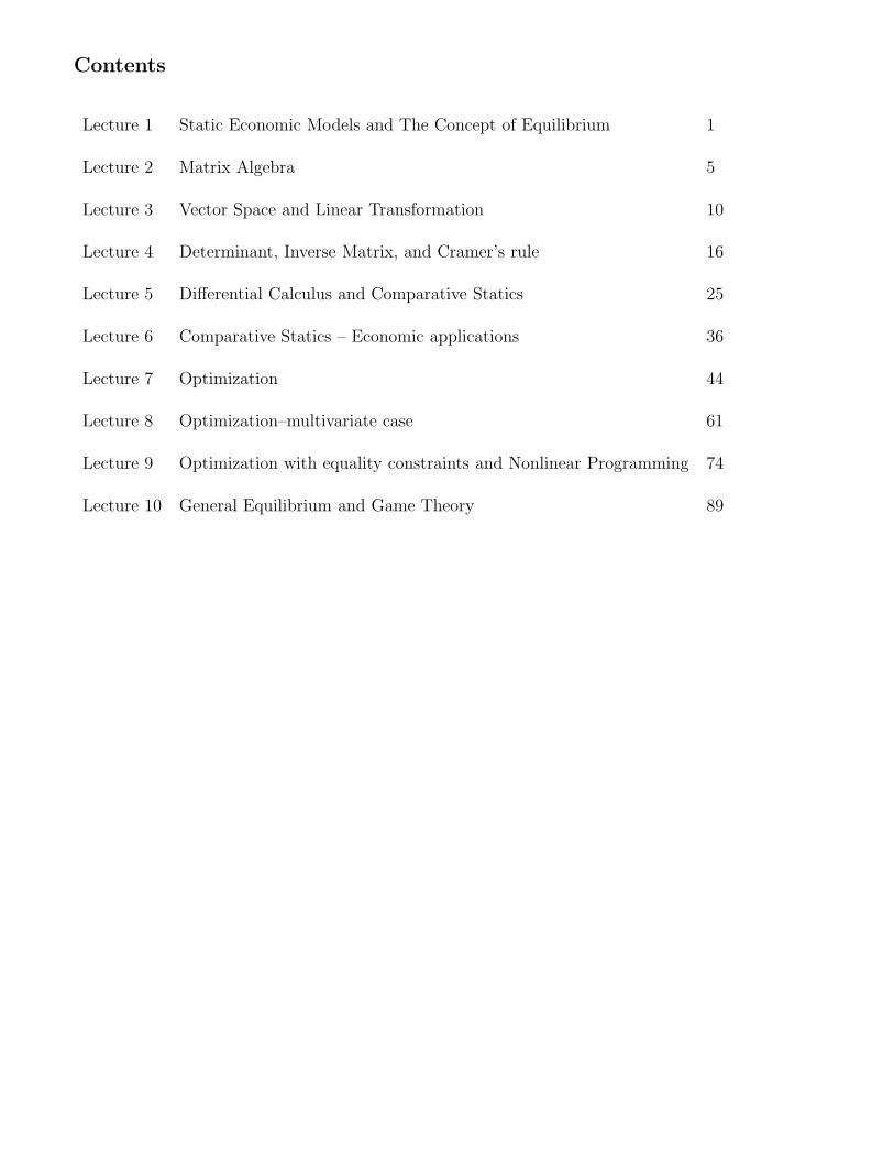
Contents
Lecture 1 Static Economic Models and The Concept of Equilibrium 1
Lecture 2 Matrix Algebra 5
Lecture 3 Vector Space and Linear Transformation 10
Lecture 4 Determinant, Inverse Matrix, and Cramer’s rule 16
Lecture 5 Differential Calculus and Comparative Statics 25
Lecture 6 Comparative Statics – Economic applications 36
Lecture 7 Optimization 44
Lecture 8 Optimization–multivariate case 61
Lecture 9 Optimization with equality constraints and Nonlinear Programming 74
Lecture 10 General Equilibrium and Game Theory 89

1
1 Static Economic Models and The Concept of Equilibrium
Here we use three elementary examples to illustrate the general structure of an eco-nomic model.
1.1 Partial market equilibrium model
A partial market equilibrium model is constructed to explain the determination ofthe price of a certain commodity. The abstract form of the model is as follows.
Qd = D(P ; a) Qs = S(P ; a) Qd = Qs,
Qd: quantity demanded of the commodity D(P ; a): demand functionQs: quantity supplied to the market S(P ; a): supply functionP : market price of the commoditya: a factor that affects demand and supply
Equilibrium: A particular state that can be maintained.Equilibrium conditions: Balance of forces prevailing in the model.Substituting the demand and supply functions, we have D(P ; a) = S(P ; a).For a given a, we can solve this last equation to obtain the equilibrium price P ∗ asa function of a. Then we can study how a affects the market equilibrium price byinspecting the function.
Example: D(P ; a) = a2/P , S(P ) = 0.25P . a2/P ∗ = 0.25P ∗ ⇒ P ∗ = 2a, Q∗d = Q∗
s =0.5a.
1.2 General equilibrium model
Usually, markets for different commodities are interrelated. For example, the priceof personal computers is strongly influenced by the situation in the market of micro-processors, the price of chicken meat is related to the supply of pork, etc. Therefore,we have to analyze interrelated markets within the same model to be able to capturesuch interrelationship and the partial equilibrium model is extended to the generalequilibrium model. In microeconomics, we even attempt to include every commodity(including money) in a general equilibrium model.Qd1 = D1(P1, . . . , Pn; a)Qs1 = S1(P1, . . . , Pn; a)
Qd1 = Qs1
Qd2 = D2(P1, . . . , Pn; a)Qs2 = S2(P1, . . . , Pn; a)
Qd2 = Qs2
. . . Qdn = Dn(P1, . . . , Pn; a)Qsn = Sn(P1, . . . , Pn; a)
Qdn = Qsn
Qdi: quantity demanded of commodity iQsi: quantity supplied of commodity iPi: market price of commodity ia: a factor that affects the economy
Di(P1, . . . , Pn; a): demand function of commodity iSi(P1, . . . , Pn; a): supply function of commodity i
We have three variables and three equations for each commodity/market.
2
Substituting the demand and supply functions, we have
D1(P1, . . . , Pn; a)− S1(P1, . . . , Pn; a) ≡ E1(P1, . . . , Pn; a) = 0D2(P1, . . . , Pn; a)− S2(P1, . . . , Pn; a) ≡ E2(P1, . . . , Pn; a) = 0
......
Dn(P1, . . . , Pn; a)− Sn(P1, . . . , Pn; a) ≡ En(P1, . . . , Pn; a) = 0.
For a given a, it is a simultaneous equation in (P1, . . . , Pn). There are n equationsand n unknown. In principle, we can solve the simultaneous equation to find theequilibrium prices (P ∗
1 , . . . , P ∗n).
A 2-market linear model:D1 = a0 + a1P1 + a2P2, S1 = b0 + b1P1 + b2P2, D2 = α0 + α1P1 + α2P2, S2 =β0 + β1P1 + β2P2.
(a0 − b0) + (a1 − b1)P1 + (a2 − b2)P2 = 0(α0 − β0) + (α1 − β1)P1 + (α2 − β2)P2 = 0.
1.3 National income model
The most fundamental issue in macroeconomics is the determination of the nationalincome of a country.
C = a + bY (a > 0, 0 < b < 1)I = I(r)Y = C + I + GS = Y − C.
C: Consumption Y : National incomeI: Investment S: SavingsG: government expenditure r: interest rate
a, b: coefficients of the consumption function.
To solve the model, we substitute the first two equations into the third to obtainY = a + bY + I0 + G⇒ Y ∗ = (a + I(r) + G)/(1− b).
1.4 The ingredients of a model
We set up economic models to study economic phenomena (cause-effect relation-ships), or how certain economic variables affect other variables. A model consists ofequations, which are relationships among variables.
Variables can be divided into three categories:Endogenous variables: variables we choose to represent different states of a model.Exogenous variables: variables assumed to affect the endogenous variables but arenot affected by them.Causes (Changes in exogenous var.) ⇒ Effects (Changes in endogenous var.)Parameters: Coefficients of the equations.
3
End. Var. Ex. Var. ParametersPartial equilibrium model: P , Qd, Qs a Coefficients of D(P ; a), S(P ; a)General equilibrium model: Pi, Qdi, Qsi aIncome model: C, Y , I, S r, G a, b
Equations can be divided into three types:Behavioral equations: representing the decisions of economic agents in the model.Equilibrium conditions: the condition such that the state can be maintained (whendifferent forces/motivations are in balance).Definitions: to introduce new variables into the model.
Behavioral equations Equilibrium cond. DefinitionsPartial equilibrium model: Qd = D(P ; a), Qs = S(P ; a) Qd = Qs
General equilibrium model: Qdi = Di(P1, . . . , Pn), Qdi = Qsi
Qsi = Si(P1, . . . , Pn)Income model: C = a + bY , I = I(r) Y = C + I + G S = Y − C
1.5 The general economic model
Assume that there are n endogenous variables and m exogenous variables.Endogenous variables: x1, x2, . . . , xn
Exogenous variables: y1, y2, . . . , ym.There should be n equations so that the model can be solved.
F1(x1, x2, . . . , xn; y1, y2, . . . , ym) = 0F2(x1, x2, . . . , xn; y1, y2, . . . , ym) = 0
...Fn(x1, x2, . . . , xn; y1, y2, . . . , ym) = 0.
Some of the equations are behavioral, some are equilibrium conditions, and some aredefinitions.
In principle, given the values of the exogenous variables, we solve to find theendogenous variables as functions of the exogenous variables:
x1 = x1(y1, y2, . . . , ym)x2 = x1(y1, y2, . . . , ym)
...xn = x1(y1, y2, . . . , ym).
If the equations are all linear in (x1, x2, . . . , xn), then we can use Cramer’s rule (tobe discussed in the next part) to solve the equations. However, if some equations arenonlinear, it is usually very difficult to solve the model. In general, we use comparativestatics method (to be discussed in part 3) to find the differential relationships betweenxi and yj:
∂xi
∂yj.
4
1.6 Problems
1. Find the equilibrium solution of the following model:
Qd = 3− P 2, Qs = 6P − 4, Qs = Qd.
2. The demand and supply functions of a two-commodity model are as follows:
Qd1 = 18− 3P1 + P2 Qd2 = 12 + P1 − 2P2
Qs1 = −2 + 4P1 Qs2 = −2 + 3P2
Find the equilibrium of the model.
3. (The effect of a sales tax) Suppose that the government imposes a sales tax oft dollars per unit on product 1. The partial market model becomes
Qd1 = D(P1 + t), Qs
1 = S(P1), Qd1 = Qs
1.
Eliminating Qd1 and Qs
1, the equilibrium price is determined by D(P1 + t) =S(P1).
(a) Identify the endogenous variables and exogenous variable(s).
(b) Let D(p) = 120−P and S(p) = 2P . Calculate P1 and Q1 both as functionof t.
(c) If t increases, will P1 and Q1 increase or decrease?
4. Let the national-income model be:
Y = C + I0 + GC = a + b(Y − T0) (a > 0, 0 < b < 1)G = gY (0 < g < 1)
(a) Identify the endogenous variables.
(b) Give the economic meaning of the parameter g.
(c) Find the equilibrium national income.
(d) What restriction(s) on the parameters is needed for an economically rea-sonable solution to exist?
5. Find the equilibrium Y and C from the following:
Y = C + I0 + G0, C = 25 + 6Y 1/2, I0 = 16, G0 = 14.
6. In a 2-good market equilibrium model, the inverse demand functions are givenby
P1 = Q−2
3
1 Q1
3
2 , P2 = Q1
3
1 Q−2
3
2 .
(a) Find the demand functions Q1 = D1(P1, P2) and Q2 = D2(P1, P2).
(b) Suppose that the supply functions are
Q1 = a−1P1, Q2 = P2.
Find the equilibrium prices (P ∗1 , P ∗
2 ) and quantities (Q∗1, Q
∗2) as functions
of a.
5
2 Matrix Algebra
A matrix is a two dimensional rectangular array of numbers:
A ≡
a11 a12 . . . a1n
a21 a22 . . . a2n...
.... . .
...am1 am2 . . . amn
There are n columns each with m elements or m rows each with n elements. We saythat the size of A is m× n.If m = n, then A is a square matrix.A m× 1 matrix is called a column vector and a 1× n matrix is called a row vector.A 1× 1 matrix is just a number, called a scalar number.
2.1 Matrix operations
Equality: A = B ⇒ (1) size(A) = size(B), (2) aij = bij for all ij.Addition/subtraction: A+B and A−B can be defined only when size(A) = size(B),in that case, size(A+B) = size(A−B) = size(A) = size(B) and (A+B)ij = aij + bij ,(A− B)ij = aij − bij . For example,
A =
(
1 23 4
)
, B =
(
1 00 1
)
⇒ A + B =
(
2 23 5
)
, A− B =
(
0 23 3
)
.
Scalar multiplication: The multiplication of a scalar number α and a matrix A,denoted by αA, is always defined with size (αA) = size(A) and (αA)ij = αaij. For
example, A =
(
1 23 4
)
, ⇒ 4A =
(
4 812 16
)
.
Multiplication of two matrices: Let size(A) = m × n and size(B) = o × p, themultiplication of A and B, C = AB, is more complicated. (1) it is not always defined.(2) AB 6= BA even when both are defined. The condition for AB to be meaningfulis that the number of columns of A should be equal to the number of rows of B, i.e.,n = o. In that case, size (AB) = size (C) = m× p.
A =
a11 a12 . . . a1n
a21 a22 . . . a2n...
.... . .
...am1 am2 . . . amn
, B =
b11 b12 . . . b1p
b21 b22 . . . a2p...
.... . .
...bn1 bn2 . . . anp
⇒C =
c11 c12 . . . c1p
c21 c22 . . . c2p...
.... . .
...cm1 cm2 . . . cmp
,
where cij =∑n
k=1 aikbkj .
Examples:
(
1 20 5
)(
34
)
=
(
3 + 80 + 20
)
=
(
1120
)
,(
1 23 4
)(
5 67 8
)
=
(
5 + 14 6 + 1615 + 28 18 + 32
)
=
(
19 2243 50
)
,

6
(
5 67 8
)(
1 23 4
)
=
(
5 + 18 10 + 247 + 24 14 + 32
)
=
(
23 3431 46
)
.
Notice that
(
1 23 4
)(
5 67 8
)
6=(
5 67 8
)(
1 23 4
)
.
2.2 Matrix representation of a linear simultaneous equation system
A linear simultaneous equation system:
a11x1 + . . . + a1nxn = b1...
...an1x1 + . . . + annxn = bn
Define A ≡
a11 . . . a1n...
. . ....
an1 . . . ann
, x ≡
x1...
xn
and b ≡
b1...bn
. Then the equation
Ax = b is equivalent to the simultaneous equation system.
Linear 2-market model:
E1 = (a1 − b1)p1 + (a2 − b2)p2 + (a0 − b0) = 0E2 = (α1 − β1)p1 + (α2 − β2)p2 + (α0 − β0) = 0
⇒(
a1 − b1 a2 − b2
α1 − β1 α2 − β2
)(
p1
p2
)
+
(
a0 − b0
α0 − β0
)
=
(
00
)
.
Income determination model:
C = a + bYI = I(r)
Y = C + I⇒
1 0 −b0 1 01 1 −1
CIY
=
aI(r)0
.
In the algebra of real numbers, the solution to the equation ax = b is x = a−1b.In matrix algebra, we wish to define a concept of A−1 for a n × n matrix A so thatx = A−1b is the solution to the equation Ax = b.
2.3 Commutative, association, and distributive laws
The notations for some important sets are given by the following table.N = nature numbers 1, 2, 3, . . . I = integers . . . ,−2,−1, 0, 1, 2, . . .Q = rational numbers m
nR = real numbers
Rn = n-dimensional column vectors M(m, n) = m× n matricesM(n) = n× n matrices
A binary operation is a law of composition of two elements from a set to form athird element of the same set. For example, + and × are binary operations of realnumbers R.Another important example: addition and multiplication are binary operations of ma-trices.

7
Commutative law of + and × in R: a + b = b + a and a× b = b× a for all a, b ∈ R.Association law of + and × in R: (a+ b)+ c = a+(b+ c) and (a× b)× c = a× (b× c)for all a, b, c ∈ R.Distributive law of + and × in R: (a+b)×c = a×c+b×c and c×(a+b) = c×a+c×bfor all a, b, c ∈ R.The addition of matrices satisfies both commutative and associative laws: A + B =B + A and (A + B) + C = A + (B + C) for all A, B, C ∈ M(m, n). The proof istrivial.In an example, we already showed that the matrix multiplication does not satisfy thecommutative law AB 6= BA even when both are meaningful.Nevertheless the matrix multiplication satisfies the associative law (AB)C = A(BC)when the sizes are such that the multiplications are meaningful. However, this de-serves a proof!It is also true that matrix addition and multiplication satisfy the distributive law:(A + B)C = AC + BC and C(A + B) = CA + CB. You should try to prove thesestatements as exercises.
2.4 Special matrices
In the space of real numbers, 0 and 1 are very special. 0 is the unit element of + and1 is the unit element of ×: 0+a = a+0 = a, 0×a = a×0 = 0, and 1×a = a×1 = a.In matrix algebra, we define zero matrices and identity matrices as
Om,n ≡
0 . . . 0...
. . ....
0 . . . 0
In ≡
1 0 . . . 00 1 . . . 0...
.... . .
...0 0 . . . 1
.
Clearly, O+A = A+O = A, OA = AO = O, and IA = AI = A. In the multiplication
of real numbers if a, b 6= 0 then a×b 6= 0. However,
(
1 00 0
)(
0 00 1
)
=
(
0 00 0
)
=
O2,2.Idempotent matrix: If AA = A (A must be square), then A is an idempotent matrix.
Both On,n and In are idempotent. Another example is A =
(
0.5 0.50.5 0.5
)
.
Transpose of a matrix: For a matrix A with size m × n, we define its transpose A′
as a matrix with size n ×m such that the ij-th element of A′ is equal to the ji-thelement of A, a′
ij = aji.
A =
(
1 2 34 5 6
)
then A′ =
1 42 53 6
.
Properties of matrix transposition:(1) (A′)′ = A, (2) (A + B)′ = A′ + B′, (3) (AB)′ = B′A′.Symmetrical matrix: If A = A′ (A must be square), then A is symmetrical. The

8
condition for A to be symmetrical is that aij = aji. Both On,n and In are symmetrical.
Another example is A =
(
1 22 3
)
.
Projection matrix: A symmetrical idempotent matrix is a projection matrix.Diagonal matrix: A symmetrical matrix A is diagonal if aij = 0 for all i 6= j. Both
In and On,n are diagonal. Another example is A =
λ1 0 00 λ2 00 0 λ3
2.5 Inverse of a square matrix
We are going to define the inverse of a square matrix A ∈M(n).Scalar: aa−1 = a−1a = 1⇒ if b satisfies ab = ba = 1 then b = a−1.Definition of A−1: If there exists a B ∈ M(n) such that AB = BA = In, then wedefine A−1 = B.Examples: (1) Since II = I, I−1 = I. (2) On,nB = On,n ⇒ O−1
n,n does not exist. (3)
If A =
(
a1 00 a2
)
, a1, a2 6= 0, then A−1 =
(
a−11 00 a−1
2
)
. (4) If a1 = 0 or a2 = 0,
then A−1 does not exist.Singular matrix: A square matrix whose inverse matrix does not exist.Non-singular matrix: A is non-singular if A−1 exists.
Properties of matrix inversion:Let A, B ∈M(n), (1) (A−1)−1 = A, (2) (AB)−1 = B−1A−1, (3) (A′)−1 = (A−1)′.
2.6 Problems
1. Let A = I −X(X ′X)−1X ′.(a) If the dimension of X is m× n, what must be the dimension of I and A.(b) Show that matrix A is idempotent.
2. Let A and B be n× n matrices and I be the identity matrix.(a) (A + B)3 = ?(b) (A + I)3 = ?
3. Let B =
((
0.5 0.50.5 0.5
))
, U = (1, 1)′, V = (1,−1)′, and W = aU + bV , where
a and b are real numbers. Find BU , BV , and BW . Is B idempotent?
4. Suppose A is a n× n nonsingular matrix and P is a n× n idempotent matrix.Show that APA−1 is idempotent.
5. Suppose that A and B are n×n symmetric idempotent matrices and AB = B.Show that A− B is idempotent.
6. Calculate (x1, x2)
(
3 22 5
)(
x1
x2
)
.
9
7. Let I =
(
1 00 1
)
and J =
(
0 1−1 0
)
.
(a) Show that J2 = −I.
(b) Make use of the above result to calculate J3, J4, and J−1.
(c) Show that (aI + bJ)(cI + dJ) = (ac− bd)I + (ad + bc)J .
(d) Show that (aI + bJ)−1 =1
a2 + b2(aI − bJ) and [(cos θ)I + (sin θ)J ]−1 =
(cos θ)I − (sin θ)J .
10
3 Vector Space and Linear Transformation
In the last section, we regard a matrix simply as an array of numbers. Now we aregoing to provide some geometrical meanings to a matrix.(1) A matrix as a collection of column (row) vectors(2) A matrix as a linear transformation from a vector space to another vector space
3.1 Vector space, linear combination, and linear independence
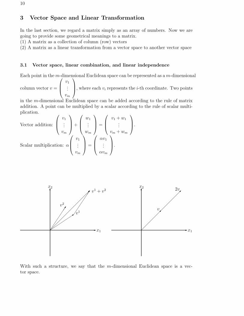
Each point in the m-dimensional Euclidean space can be represented as a m-dimensional
column vector v =
v1...
vm
, where each vi represents the i-th coordinate. Two points
in the m-dimensional Euclidean space can be added according to the rule of matrixaddition. A point can be multiplied by a scalar according to the rule of scalar multi-plication.
Vector addition:
v1...
vm
+
w1...
wm
=
v1 + w1...
vm + wm
.
Scalar multiplication: α
v1...
vm
=
αv1...
αvm
.
- x1
6x2
��
��
��3
v1
�
�
v2
��
��
��
��
��� v1 + v2
- x1
6x2
��
��
��v �
��
���
2v
With such a structure, we say that the m-dimensional Euclidean space is a vec-tor space.

11
m-dimensional column vector space: Rm =
v1...
vm
, vi ∈ R
.
We use superscripts to represent individual vectors.
A m× n matrix: a collection of n m-dimensional column vectors:
a11 a12 . . . a1n
a21 a22 . . . a2n...
.... . .
...am1 am2 . . . amn
=
a11
a21...
am1
,
a12
a22...
am2
, . . . ,
a1n
a2n...
amn
Linear combination of a collection of vectors {v1, . . . , vn}: w =
n∑
i=1
αivi, where
(α1, . . . , αn) 6= (0, . . . , 0).
Linear dependence of {v1, . . . , vn}: If one of the vectors is a linear combination ofothers, then the collection is said to be linear dependent. Alternatively, the collectionis linearly dependent if (0, . . . , 0) is a linear combination of it.
Linear independence of {v1, . . . , vn}: If the collection is not linear dependent, thenit is linear independent.
Example 1: v1 =
a1
00
, v2 =
0a2
0
, v3 =
00a3
, a1a2a3 6= 0.
If α1v1 + α2v
2 + α3v3 = 0 then (α1, α2, α3) = (0, 0, 0). Therefore, {v1, v2, v3} must be
linear independent.
Example 2: v1 =
123
, v2 =
456
, v3 =
789
.
2v2 = v1 + v3. Therefore, {v1, v2, v3} is linear dependent.
Example 3: v1 =
123
, v2 =
456
.
α1v1 + α2v
2 =
α1 + 4α2
2α1 + 5α2
3α1 + 6α2
=
000
⇒ α1 = α2 = 0. Therefore, {v1, v2} is
linear independent.
Span of {v1, . . . , vn}: The space of linear combinations.If a vector is a linear combination of other vectors, then it can be removed withoutchanging the span.

12
Rank
v11 . . . v1n...
. . ....
vm1 . . . vmn
≡ Dimension(Span{v1, . . . , vn}) = Maximum # of indepen-
dent vectors.
3.2 Linear transformation
Consider a m × n matrix A. Given x ∈ Rn, Ax ∈ Rm. Therefore, we can define alinear transformation from Rn to Rm as f(x) = Ax or
f : Rn→Rm, f(x) =
y1...
ym
=
a11 . . . a1n...
. . ....
am1 . . . amn
x1...
xn
.
It is linear because f(αx + βw) = A(αx + βw) = αAx + βAw = αf(x) + βf(w).
Standard basis vectors of Rn: e1 ≡
10...0
, e2 ≡
01...0
, . . . , en ≡
00...1
.
Let vi be the i-th column of A, vi =
a1i...
ami
.
vi = f(ei):
a11
. . .am1
=
a11 . . . a1n...
. . ....
am1 . . . amn
1...0
⇒ v1 = f(e1) = Ae1, etc.
Therefore, vi is the image of the i-th standard basis vector ei under f .Span{v1, . . . , vn} = Range space of f(x) = Ax ≡ R(A).Rank(A) ≡ dim(R(A)).Null space of f(x) = Ax: N(A) ≡ {x ∈ Rn, f(x) = Ax = 0}.dim(R(A)) + dim(N(A)) = n.
Example 1: A =
(
1 00 2
)
. N(A) =
{(
00
)}
, R(A) = R2, Rank(A) = 2.
Example 2: B =
(
1 11 1
)
. N(B) =
{(
k−k
)
, k ∈ R
}
, R(B) =
{(
kk
)
, k ∈ R
}
,
Rank(B) = 1.
The multiplication of two matrices can be interpreted as the composition of twolinear transformations.
f : Rn→Rm, f(x) = Ax, g : Rp→Rn, g(y) = By, ⇒ f(g(x)) = A(By), f◦g : Rp→Rm.

13
The composition is meaningful only when the dimension of the range space of g(y)is equal to the dimension of the domain of f(x), which is the same condition for thevalidity of the matrix multiplication.
Every linear transformation f : Rn→Rm can be represented by f(x) = Ax forsome m× n matrix.
3.3 Inverse transformation and inverse of a square matrix
Consider now the special case of square matrices. Each A ∈ M(n) represents a lineartransformation f : Rn→Rn.The definition of the inverse matrix A−1 is such that AA−1 = A−1A = I. If we re-gard A as a linear transformation from Rn→Rn and I as the identity transformationthat maps every vector (point) into itself, then A−1 is the inverse mapping of A. Ifdim(N(A)) = 0, then f(x) is one to one.If dim(R(A)) = n, then R(A) = Rn and f(x) is onto.⇒ if Rank(A) = n, then f(x) is one to one and onto and there exits an inverse mappingf−1 : Rn→Rn represented by a n×n square matrix A−1. f−1f(x) = x⇒ A−1Ax = x.⇒ if Rank(A) = n, then A is non-singular.if Rank(A) < n, then f(x) is not onto, no inverse mapping exists, and A is singular.
Examples: Rank
a1 0 00 a2 00 0 a3
= 3 and Rank
1 4 72 5 83 6 9
= 2.
Remark: On,n represents the mapping that maps every point to the origin. In rep-resents the identity mapping that maps a point to itself. A projection matrix repre-
sents a mapping that projects points onto a linear subspace of Rn, eg.,
(
0.5 0.50.5 0.5
)
projects points onto the 45 degree line.
- x1
6x2
��
��
��
��
��
��
��
��
��
��
�
@@
@@
@@
@@I
@@
@@
@@
@@R
@@R
x
Ax
x =
(
12
)
Ax =
(
.5 .5
.5 .5
)(
12
)
=
(
1.51.5
)
x′ =
(
k−k
)
, Ax′ =
(
00
)
14
3.4 Problems
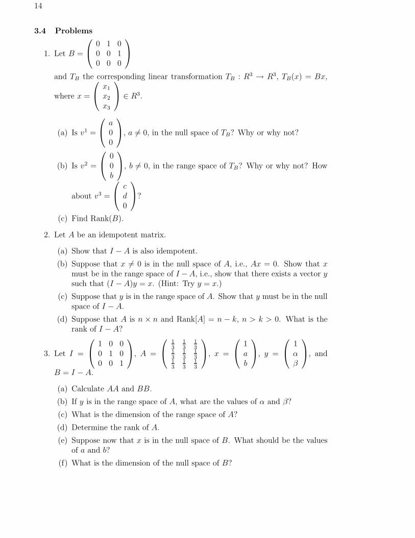
1. Let B =
0 1 00 0 10 0 0
and TB the corresponding linear transformation TB : R3 → R3, TB(x) = Bx,
where x =
x1
x2
x3
∈ R3.
(a) Is v1 =
a00
, a 6= 0, in the null space of TB? Why or why not?
(b) Is v2 =
00b
, b 6= 0, in the range space of TB? Why or why not? How
about v3 =
cd0
?
(c) Find Rank(B).
2. Let A be an idempotent matrix.
(a) Show that I − A is also idempotent.
(b) Suppose that x 6= 0 is in the null space of A, i.e., Ax = 0. Show that xmust be in the range space of I −A, i.e., show that there exists a vector ysuch that (I −A)y = x. (Hint: Try y = x.)
(c) Suppose that y is in the range space of A. Show that y must be in the nullspace of I − A.
(d) Suppose that A is n × n and Rank[A] = n − k, n > k > 0. What is therank of I − A?
3. Let I =
1 0 00 1 00 0 1
, A =
13
13
13
13
13
13
13
13
13
, x =
1ab
, y =
1αβ
, and
B = I − A.
(a) Calculate AA and BB.
(b) If y is in the range space of A, what are the values of α and β?
(c) What is the dimension of the range space of A?
(d) Determine the rank of A.
(e) Suppose now that x is in the null space of B. What should be the valuesof a and b?
(f) What is the dimension of the null space of B?
15
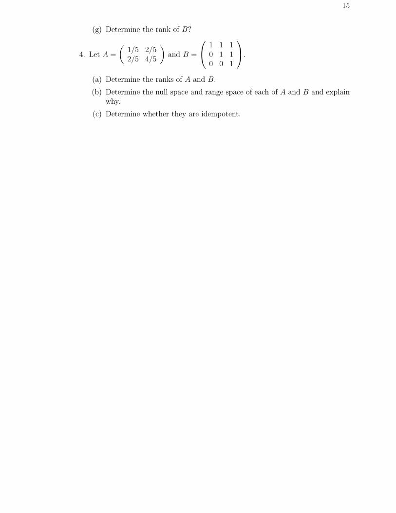
(g) Determine the rank of B?
4. Let A =
(
1/5 2/52/5 4/5
)
and B =
1 1 10 1 10 0 1
.
(a) Determine the ranks of A and B.
(b) Determine the null space and range space of each of A and B and explainwhy.
(c) Determine whether they are idempotent.
16
4 Determinant, Inverse Matrix, and Cramer’s rule
In this section we are going to derive a general method to calculate the inverse ofa square matrix. First, we define the determinant of a square matrix. Using theproperties of determinants, we find a procedure to compute the inverse matrix. Thenwe derive a general procedure to solve a simultaneous equation.
4.1 Permutation group
A permutation of {1, 2, . . . , n} is a 1-1 mapping of {1, 2, . . . , n} onto itself, written as
π =
(
1 2 . . . ni1 i2 . . . in
)
meaning that 1 is mapped to i1, 2 is mapped to i2, . . ., and
n is mapped to in. We also write π = (i1, i2, . . . , ın) when no confusing.
Permutation set of {1, 2, . . . , n}: Pn ≡ {π = (i1, i2, . . . , in) : π is a permutation}.P2 = {(1, 2), (2, 1)}.P3 = {(1, 2, 3), (1, 3, 2), (2, 1, 3), (2, 3, 1), (3, 1, 2), (3, 2, 1)}.P4: 4! = 24 permutations.
Inversions in a permutation π = (i1, i2, . . . , in): If there exist k and l such thatk < l and ik > il, then we say that an inversion occurs.N(i1, i2, . . . , ın): Total number of inversions in (i1, i2, . . . , in).Examples: 1. N(1, 2) = 0, N(2, 1) = 1.
2. N(1, 2, 3) = 0, N(1, 3, 2) = 1, N(2, 1, 3) = 1,N(2, 3, 1) = 2, N(3, 1, 2) = 2, N(3, 2, 1) = 3.
4.2 Determinant
Determinant of A =
a11 a12 . . . a1n
a21 a22 . . . a2n...
.... . .
...an1 an2 . . . ann
:
|A| ≡∑
(i1,i2,...,in)∈Pn
(−1)N(i1,i2,...,in)a1i1a2i2 . . . anin .
n = 2:
∣
∣
∣
∣
a11 a12
a21 a22
∣
∣
∣
∣
= (−1)N(1,2)a11a22 + (−1)N(2,1)a12a21 = a11a22 − a12a21.
n = 3:
∣
∣
∣
∣
∣
∣
a11 a12 a13
a21 a22 a23
a31 a32 a33
∣
∣
∣
∣
∣
∣
=
(−1)N(1,2,3)a11a22a33 + (−1)N(1,3,2)a11a23a32 + (−1)N(2,1,3)a12a21a33 +(−1)N(2,3,1)a12a23a31 + (−1)N(3,1,2)a13a21a32 + (−1)N(3,2,1)a13a22a31
= a11a22a33 − a11a23a32 − a12a21a33 + a12a23a31 + a13a21a32 − a13a22a31.
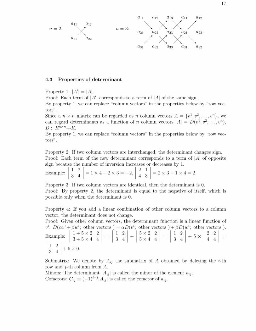
17
a11 a12
a21 a22
@@R���n = 2:
a11 a12 a13 a11 a12
a21 a22 a23 a21 a22
a31 a32 a33 a31 a32
@@R
@@R
@@R
@@R
@@R
@@R
���
���
���
���
���
���
n = 3:
4.3 Properties of determinant
Property 1: |A′| = |A|.Proof: Each term of |A′| corresponds to a term of |A| of the same sign.By property 1, we can replace “column vectors” in the properties below by “row vec-tors”.Since a n × n matrix can be regarded as n column vectors A = {v1, v2, . . . , vn}, wecan regard determinants as a function of n column vectors |A| = D(v1, v2, . . . , vn),D : Rn×n→R.By property 1, we can replace “column vectors” in the properties below by “row vec-tors”.
Property 2: If two column vectors are interchanged, the determinant changes sign.Proof: Each term of the new determinant corresponds to a term of |A| of oppositesign because the number of inversion increases or decreases by 1.
Example:
∣
∣
∣
∣
1 23 4
∣
∣
∣
∣
= 1× 4− 2× 3 = −2,
∣
∣
∣
∣
2 14 3
∣
∣
∣
∣
= 2× 3− 1× 4 = 2,
Property 3: If two column vectors are identical, then the determinant is 0.Proof: By property 2, the determinant is equal to the negative of itself, which ispossible only when the determinant is 0.
Property 4: If you add a linear combination of other column vectors to a columnvector, the determinant does not change.Proof: Given other column vectors, the determinant function is a linear function ofvi: D(αvi + βwi; other vectors ) = αD(vi; other vectors ) + βD(wi; other vectors ).
Example:
∣
∣
∣
∣
1 + 5× 2 23 + 5× 4 4
∣
∣
∣
∣
=
∣
∣
∣
∣
1 23 4
∣
∣
∣
∣
+
∣
∣
∣
∣
5× 2 25× 4 4
∣
∣
∣
∣
=
∣
∣
∣
∣
1 23 4
∣
∣
∣
∣
+ 5 ×∣
∣
∣
∣
2 24 4
∣
∣
∣
∣
=∣
∣
∣
∣
1 23 4
∣
∣
∣
∣
+ 5× 0.
Submatrix: We denote by Aij the submatrix of A obtained by deleting the i-throw and j-th column from A.Minors: The determinant |Aij| is called the minor of the element aij .Cofactors: Cij ≡ (−1)i+j|Aij | is called the cofactor of aij .

18
Property 5 (Laplace theorem): Given i = i, |A| =n∑
j=1
aijCij.
Given j = j, |A| = ∑ni=1 aijCij.
Proof: In the definition of the determinant of |A|, all terms with aij can be put to-gethere to become aijCij.
Example:
∣
∣
∣
∣
∣
∣
1 2 34 5 67 8 0
∣
∣
∣
∣
∣
∣
= 1×∣
∣
∣
∣
5 68 0
∣
∣
∣
∣
− 2×∣
∣
∣
∣
4 67 0
∣
∣
∣
∣
+ 3×∣
∣
∣
∣
4 57 8
∣
∣
∣
∣
.
Property 6: Given i′ 6= i,n∑
j=1
ai′jCij = 0.
Given j′ 6= j, =∑n
i=1 aij′Cij = 0.Therefore, if you multiply cofactors by the elements from a different row or column,you get 0 instead of the determinant.Proof: The sum becomes the determinant of a matrix with two identical rows (columns).
Example: 0 = 4×∣
∣
∣
∣
5 68 0
∣
∣
∣
∣
− 5×∣
∣
∣
∣
4 67 0
∣
∣
∣
∣
+ 6×∣
∣
∣
∣
4 57 8
∣
∣
∣
∣
.
4.4 Computation of the inverse matrix
Using properties 5 and 6, we can calculate the inverse of A as follows.
1. Cofactor matrix: C ≡
C11 C12 . . . C1n
C21 C22 . . . C2n...
.... . .
...Cn1 Cn2 . . . Cnn
.
2. Adjoint of A: Adj A ≡ C ′ =
C11 C21 . . . Cn1
C12 C22 . . . Cn2...
.... . .
...C1n C2n . . . Cnn
.
3. ⇒ AC ′ = C ′A =
|A| 0 . . . 00 |A| . . . 0...
.... . .
...0 0 . . . |A|
⇒ if |A| 6= 0 then 1|A|C
′ = A−1.
Example 1: A =
(
a11 a12
a21 a22
)
then C =
(
a22 −a21
−a12 a11
)
.
A−1 =1
|A|C′ =
1
a11a22 − a12a21
(
a22 −a12
−a21 a11
)
; if |A| = a11a22 − a12a21 6= 0.
Example 2: A =
1 2 34 5 67 8 0
⇒ |A| = 27 6= 0 and
C11 =
∣
∣
∣
∣
5 68 0
∣
∣
∣
∣
= −48, C12 = −∣
∣
∣
∣
4 67 0
∣
∣
∣
∣
= 42, C13 =
∣
∣
∣
∣
4 57 8
∣
∣
∣
∣
= −3,
19
C21 = −∣
∣
∣
∣
2 38 0
∣
∣
∣
∣
= 24, C22 =
∣
∣
∣
∣
1 37 0
∣
∣
∣
∣
= −21, C23 = −∣
∣
∣
∣
1 27 8
∣
∣
∣
∣
= 6,
C31 =
∣
∣
∣
∣
2 35 6
∣
∣
∣
∣
= −3, C32 = −∣
∣
∣
∣
1 34 6
∣
∣
∣
∣
= 6, C33 =
∣
∣
∣
∣
1 24 5
∣
∣
∣
∣
= −3,
C =
−48 42 −324 −21 6−3 6 −3
, C ′ =
−48 24 −342 −21 6−3 6 −3
, A−1 =1
27
−48 24 −342 −21 6−3 6 −3
.
If |A| = 0, then A is singular and A−1 does not exist. The reason is that |A| =
0⇒ AC ′ = 0n×n ⇒ C11
a11...
an1
+ · · ·+Cn1
a1n...
ann
=
0...0
. The column vectors
of A are linear dependent, the linear transformation TA is not onto and therefore aninverse transformation does not exist.
4.5 Cramer’s rule
If |A| 6= 0 then A is non-singular and A−1 =C ′
|A| . The solution to the simultaneous
equation Ax = b is x = A−1b =C ′b
|A| .
Cramer’s rule: xi =
∑nj=1 Cjbj
|A| =|Ai||A| , where Ai is a matrix obtained by replacing
the i-th column of A by b, Ai = {v1, . . . , vi−1, b, vi+1, . . . , vn}.
4.6 Economic applications
Linear 2-market model:
(
a1 − b1 a2 − b2
α1 − β1 α2 − β2
)(
p1
p2
)
=
(
b0 − a0
β0 − α0
)
.
p1 =
∣
∣
∣
∣
b0 − a0 a2 − b2
β0 − α0 α2 − β2
∣
∣
∣
∣
∣
∣
∣
∣
a1 − b1 a2 − b2
α1 − β1 α2 − β2
∣
∣
∣
∣
, p2 =
∣
∣
∣
∣
a1 − b1 b0 − a0
α1 − β1 β0 − α0
∣
∣
∣
∣
∣
∣
∣
∣
a1 − b1 a2 − b2
α1 − β1 α2 − β2
∣
∣
∣
∣
.
Income determination model:
1 0 −b0 1 01 1 −1
CIY
=
aI(r)0
.
C =
∣
∣
∣
∣
∣
∣
a 0 −bI(r) 1 00 1 −1
∣
∣
∣
∣
∣
∣
∣
∣
∣
∣
∣
∣
1 0 −b0 1 01 1 −1
∣
∣
∣
∣
∣
∣
, I =
∣
∣
∣
∣
∣
∣
1 a −b0 I(r) 01 0 −1
∣
∣
∣
∣
∣
∣
∣
∣
∣
∣
∣
∣
1 0 −b0 1 01 1 −1
∣
∣
∣
∣
∣
∣
, Y =
∣
∣
∣
∣
∣
∣
1 0 a0 1 I(r)1 1 0
∣
∣
∣
∣
∣
∣
∣
∣
∣
∣
∣
∣
1 0 −b0 1 01 1 −1
∣
∣
∣
∣
∣
∣
.

20
IS-LM model: In the income determination model, we regard interest rate as givenand consider only the product market. Now we enlarge the model to include themoney market and regard interest rate as the price (an endogenous variable) deter-mined in the money market.
good market: money market:C = a + bY L = kY − lRI = I0 − iR M = M
C + I + G = Y M = Lend. var: C, I, Y , R (interest rate), L(demand for money), M (money supply)ex. var: G, M (quantity of money). parameters: a, b, i, k, l.Substitute into equilibrium conditions:
good market: money market endogenous variables:a + bY + I0 − iR + G = Y , kY − lR = M , Y , R
(
1− b ik −l
)(
YR
)
=
(
a + I0 + GM
)
Y =
∣
∣
∣
∣
a + I0 + G iM −l
∣
∣
∣
∣
∣
∣
∣
∣
1− b ik −l
∣
∣
∣
∣
, R =
∣
∣
∣
∣
1− b a + I0 + Gk M
∣
∣
∣
∣
∣
∣
∣
∣
1− b ik −l
∣
∣
∣
∣
.
Two-country income determination model: Another extension of the incomedetermination model is to consider the interaction between domestic country and therest of the world (foreign country).domestic good market: foreign good market: endogenous variables:C = a + bY C ′ = a′ + b′Y ′ C, I, Y ,I = I0 I ′ = I ′
0 M (import),M = M0 + mY M ′ = M ′
0 + m′Y ′ X (export),C + I + X −M = Y C ′ + I ′ + X ′ −M ′ = Y ′ C ′, I ′, Y ′, M ′, X ′.
By definition, X = M ′ and X ′ = M . Substituting into the equilibrium conditions,
(1− b + m)Y −m′Y ′ = a + I0 + M ′0 −M0 (1− b′ + m′)Y ′ −mY = a′ + I ′
0 + M0 −M ′0.
(
1− b + m −m′
−m 1− b′ + m′
)(
YY ′
)
=
(
a + I0 + M ′0 −M0
a′ + I ′0 + M0 −M ′
0
)
.
Y =
∣
∣
∣
∣
a + I0 + M ′0 −M0 −m′
a′ + I ′0 + M0 −M ′
0 1− b′ + m′
∣
∣
∣
∣
∣
∣
∣
∣
1− b + m −m′
−m 1− b′ + m′
∣
∣
∣
∣
Y ′ =
∣
∣
∣
∣
1− b + m a + I0 + M ′0 −M0
−m a′ + I ′0 + M0 −M ′
0
∣
∣
∣
∣
∣
∣
∣
∣
1− b + m −m′
−m 1− b′ + m′
∣
∣
∣
∣
.
4.7 Input-output table
Assumption: Technologies are all fixed proportional, that is, to produce one unit ofproduct Xi, you need aji units of Xj .
21
IO table: A =
a11 a12 . . . a1n
a21 a22 . . . a2n...
.... . .
...an1 an2 . . . ann
.
Column i represents the coefficients of inputs needed to produce one unit of Xi.
Suppose we want to produce a list of outputs x =
x1
x2...
xn
, we will need a list of inputs
Ax =
a11x1 + a12x2 + . . . + a1nxn
a21x2 + a22x2 + . . . + a2nxn...
an1x1 + an2x2 + . . . + annxn
. The net output is x−Ax = (I − A)x.
If we want to produce a net amount of d =
d1
d2...
dn
, then since d = (I − A)x,
x = (I −A)−1d.
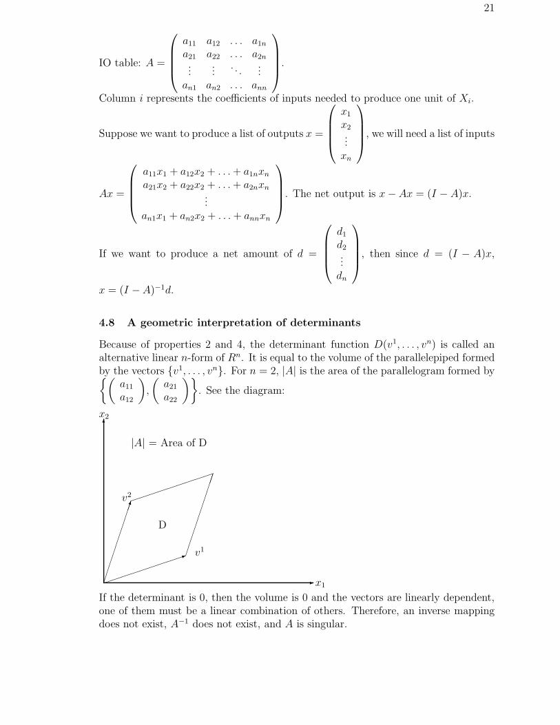
4.8 A geometric interpretation of determinants
Because of properties 2 and 4, the determinant function D(v1, . . . , vn) is called analternative linear n-form of Rn. It is equal to the volume of the parallelepiped formedby the vectors {v1, . . . , vn}. For n = 2, |A| is the area of the parallelogram formed by{(
a11
a12
)
,
(
a21
a22
)}
. See the diagram:
- x1
6x2
�����������
v2
���������1 v1
|A| = Area of D
D
���������
����������
If the determinant is 0, then the volume is 0 and the vectors are linearly dependent,one of them must be a linear combination of others. Therefore, an inverse mappingdoes not exist, A−1 does not exist, and A is singular.

22
4.9 Rank of a matrix and solutions of Ax = d when |A| = 0
Rank(A) = the maximum # of independent vectors in A = {v1, . . . , vn} = dim(RangeSpace of TA).Rank(A) = the size of the largest non-singular square submatrices of A.
Examples: Rank
(
1 23 4
)
= 2. Rank
1 2 34 5 67 8 9
= 2 because
(
1 24 5
)
is non-
singular.Property 1: Rank(AB) ≤ min{Rank(A), Rank(B)}.Property 2: dim(Null Space of TA) + dim(Range Space of TA) = n.
Consider the simultaneous equation Ax = d. When |A| = 0, there exists a row ofA that is a linear combination of other rows
and Rank(A) < n. First, form the augmented matrix M ≡ [A...d] and calculate
the rank of M . There are two cases.
Case 1: Rank(M) = Rank (A).In this case, some equations are linear combinations of others (the equations are de-pendent) and can be removed without changing the solution space. There will bemore variables than equations after removing these equations. Hence, there will beinfinite number of solutions.
Example:
(
1 22 4
)(
x1
x2
)
=
(
36
)
. Rank(A) = Rank
(
1 22 4
)
= 1 = Rank(M) =
Rank
(
1 2 32 4 6
)
.
The second equation is just twice the first equation and can be discarded. The so-
lutions are
(
x1
x2
)
=
(
3− 2kk
)
for any k. On x1-x2 space, the two equations are
represented by the same line and every point on the line is a solution.
Case 2: Rank(M) = Rank(A) + 1.In this case, there exists an equation whose LHS is a linear combination of the LHSof other equations but whose RHS is different from the same linear combination ofthe RHS of other equations. Therefore, the equation system is contraditory and therewill be no solutions.
Example:
(
1 22 4
)(
x1
x2
)
=
(
37
)
. Rank(A) = Rank
(
1 22 4
)
= 1 < Rank(M) =
Rank
(
1 2 32 4 7
)
= 2.
Multiplying the first equation by 2, 2x1 + 4x2 = 6, whereas the second equation
says 2x1 + 4x2 = 7. Therefore, it is impossible to have any
(
x1
x2
)
satisfying both
equations simultaneously. On x1-x2 space, the two equations are represented by twoparallel lines and cannot have any intersection points.
23
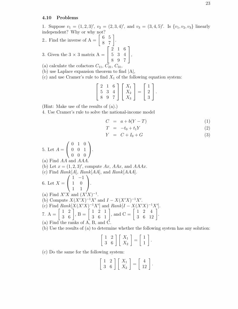
4.10 Problems
1. Suppose v1 = (1, 2, 3)′, v2 = (2, 3, 4)′, and v3 = (3, 4, 5)′. Is {v1, v2, v3} linearlyindependent? Why or why not?
2.. Find the inverse of A =
[
6 58 7
]
.
3. Given the 3 × 3 matrix A =
2 1 65 3 48 9 7
,
(a) calculate the cofactors C11, C21, C31,(b) use Laplace expansion theorem to find |A|,(c) and use Cramer’s rule to find X1 of the following equation system:
2 1 65 3 48 9 7
X1
X2
X3
=
123
.
(Hint: Make use of the results of (a).)4. Use Cramer’s rule to solve the national-income model
C = a + b(Y − T ) (1)
T = −t0 + t1Y (2)
Y = C + I0 + G (3)
5. Let A =
0 1 00 0 10 0 0
.
(a) Find AA and AAA.(b) Let x = (1, 2, 3)′, compute Ax, AAx, and AAAx.(c) Find Rank[A], Rank[AA], and Rank[AAA].
6. Let X =
1 −11 01 1
.
(a) Find X ′X and (X ′X)−1.(b) Compute X(X ′X)−1X ′ and I −X(X ′X)−1X ′.(c) Find Rank[X(X ′X)−1X ′] and Rank[I −X(X ′X)−1X ′].
7. A =
[
1 23 6
]
, B =
[
1 2 13 6 1
]
, and C =
[
1 2 43 6 12
]
.
(a) Find the ranks of A, B, and C.(b) Use the results of (a) to determine whether the following system has any solution:
[
1 23 6
] [
X1
X2
]
=
[
11
]
.
(c) Do the same for the following system:[
1 23 6
] [
X1
X2
]
=
[
412
]
.

24
8. Let A =
(
3 21 2
)
, I the 2× 2 identity matrix, and λ a scalar number.
(a) Find |A− λI|. (Hint: It is a quadratic function of λ.)(b) Determine Rank(A − I) and Rank(A − 4I). (Remark: λ = 1 and λ = 4 are theeigenvalues of A, that is, they are the roots of the equation |A− λI| = 0, called thecharacteristic equation of A.)(c) Solve the simultaneous equation system (A − I)x = 0 assuming that x1 = 1.(Remark: The solution is called an eigenvector of A associated with the eigenvalueλ = 1.)(d) Solve the simultaneous equation system (A− 4I)y = 0 assuming that y1 = 1.(e) Determine whether the solutions x and y are linearly independent.

25
5 Differential Calculus and Comparative Statics
As seen in the last chapter, a linear economic model can be represented by a matrixequation Ax = d(y) and solved using Cramer’s rule, x = A−1d(y). On the other hand,a closed form solution x = x(y) for a nonlinear economic model is, in most applica-tions, impossible to obtain. For general nonlinear economic models, we use differentialcalculus (implicit function theorem) to obtain the derivatives of endogenous variables
with respect to exogenous variables∂xi
∂yj
:
f1(x1, . . . , xn; y1, . . . , ym) = 0...
fn(x1, . . . , xn; y1, . . . , ym) = 0
⇒
∂f1
∂x1
. . .∂f1
∂xn...
. . ....
∂fn
∂x1
. . .∂fn
∂xn
∂x1
∂y1. . .
∂x1
∂ym...
. . ....
∂xn
∂y1
. . .∂xn
∂ym
= −
∂f1
∂y1. . .
∂f1
∂ym...
. . ....
∂fn
∂y1
. . .∂fn
∂ym
.
⇒
∂x1
∂y1
. . .∂x1
∂ym...
. . ....
∂xn
∂y1. . .
∂xn
∂ym
= −
∂f1
∂x1. . .
∂f1
∂xn...
. . ....
∂fn
∂x1. . .
∂fn
∂xn
−1
∂f1
∂y1
. . .∂f1
∂ym...
. . ....
∂fn
∂y1. . .
∂fn
∂ym
.
Each∂xi
∂yjrepresents a cause-effect relationship. If
∂xi
∂yj> 0 (< 0), then xi will increase
(decrease) when yj increases. Therefore, instead of computing xi = xi(y), we want to
determine the sign of∂xi
∂yj
for each i-j pair. In the following, we will explain how it
works.
5.1 Differential Calculus
x = f(y)⇒ f ′(y∗) =dx
dy
∣
∣
∣
∣
y=y∗
≡ lim∆y→0
f(y∗ + ∆y)− f(y∗)
∆y.
On y-x space, x = f(y) is represented by a curve and f ′(y∗) represents the slope ofthe tangent line of the curve at the point (y, x) = (y∗, f(y∗)).Basic rules:
1. x = f(y) = k,dx
dy= f ′(y) = 0.
2. x = f(y) = yn,dx
dy= f ′(y) = nyn−1.
3. x = cf(y),dx
dy= cf ′(y).

26
4. x = f(y) + g(y),dx
dy= f ′(y) + g′(y).
5. x = f(y)g(y),dx
dy= f ′(y)g(y) + f(y)g′(y).
6. x = f(y)/g(y),dx
dy=
f ′(y)g(y)− f(y)g′(y)
(g(y))2.
7. x = eay,dx
dy= aeay. x = ln y,
dx
dy=
1
y.
8. x = sin y,dx
dy= cos y. x = cos y,
dx
dy= − sin y.
Higher order derivatives:
f ′′(y) ≡ d
dy
(
d
dyf(y)
)
=d2
dy2f(y), f ′′′(y) ≡ d
dy
(
d2
dy2f(y)
)
=d3
dy3f(y).
5.2 Partial derivatives
In many cases, x is a function of several y’s: x = f(y1, y2, . . . , yn). The partialderivative of x with respect to yi evaluated at (y1, y2, . . . , yn) = (y∗
1, y∗2, . . . , y
∗n) is
∂x
∂yi
∣
∣
∣
∣
(y∗
1,y∗
2,...,y∗
n)
≡ lim∆yi→0
f(y∗1, . . . , y
∗i + ∆yi, . . . , y
∗n)− f(y∗
1, . . . , y∗i , . . . , y
∗n)
∆yi,
that is, we regard all other independent variables as constant (f as a function of yi
only) and take derivative.
9.∂xn
1xm2
∂x1= nxn−1
1 xm2 .
Higher order derivatives: We can define higher order derivatives as before. For thecase with two independent variables, there are 4 second order derivatives:
∂
∂y1
∂x
∂y1=
∂2x
∂y21
,∂
∂y2
∂x
∂y1=
∂2x
∂y2∂y1,
∂
∂y1
∂x
∂y2=
∂2x
∂y1∂y2,
∂
∂y2
∂x
∂y2=
∂2x
∂y22
.
Notations: f1, f2, f11, f12, f21, f22.
∇f ≡
f1...
fn
: Gradient vector of f .
H(f) ≡
f11 . . . f1n...
. . ....
fn1 . . . fnn
: second order derivative matrix, called Hessian of f .
Equality of cross-derivatives: If f is twice continously differentiable, then fij = fji
and H(f) is symmetric.
5.3 Economic concepts similar to derivatives
Elasticity of Xi w.r.t. Yj: EXi,Yj≡ Yj
Xi
∂Xi
∂Yj
, the percentage change of Xi when Yj
increases by 1 %. Example: Qd = D(P ), EQd,P =P
Qd
dQd
dP

27
Basic rules: 1. EX1X2,Y = EX1,Y + EX2,Y , 2. EX1/X2,Y = EX1,Y − EX2,Y ,3. EY,X = 1/EX,Y .
Growth rate of X = X(t): GX ≡1
X
dX
dt, the percentage change of X per unit of
time.
5.4 Mean value and Taylor’s Theorems
Continuity theorem: If f(y) is continuous on the interval [a, b] and f(a) ≤ 0, f(b) ≥ 0,then there exists a c ∈ [a, b] such that f(c) = 0.Rolle’s theorem: If f(y) is continuous on the interval [a, b] and f(a) = f(b) = 0, thenthere exists a c ∈ (a, b) such that f ′(c) = 0.
Mean value theorem: If f(y) is continously differentiable on [a, b], then there exists ac ∈ (a, b) such that
f(b)− f(a) = f ′(c)(b− a) orf(b)− f(a)
b− a= f ′(c).
Taylor’s Theorem: If f(y) is k + 1 times continously differentiable on [a, b], then foreach y ∈ [a, b], there exists a c ∈ (a, y) such that
f(y) = f(a)+f ′(a)(y−a)+f ′′(a)
2!(y−a)2 + . . .+
f (k)(a)
k!(y−a)k +
f (k+1)(c)
(k + 1)!(y−a)k+1.
5.5 Concepts of differentials and applications
Let x = f(y). Define ∆x ≡ f(y + ∆y)− f(y), called the finite difference of x.
Finite quotient:∆x
∆y=
f(y + ∆y)− f(y)
∆y⇒ ∆x =
∆x
∆y∆y.
dx, dy: Infinitesimal changes of x and y, dx, dy > 0 (so that we can divid somethingby dx or by dy) but dx, dy < a for any positive real number a (so that ∆y→dy).Differential of x = f(y): dx = df = f ′(y)dy.
Chain rule: x = f(y), y = g(z)⇒ x = f(g(z)),
dx = f ′(y)dy, dy = g′(z)dz ⇒ dx = f ′(y)g′(z)dz.dx
dz= f ′(y)g′(z) = f ′(g(z))g′(z).
Example: x = (z2 + 1)3 ⇒ x = y3, y = z2 + 1⇒ dx
dz= 3y22z = 6z(z2 + 1)2.
Inverse function rule: x = f(y), ⇒ y = f−1(x) ≡ g(x),
dx = f ′(y)dy, dy = g′(x)dx⇒ dx = f ′(y)g′(x)dx.dy
dx= g′(x) =
1
f ′(y).
Example: x = ln y ⇒ y = ex ⇒ dx
dy=
1
ex=
1
y.

28
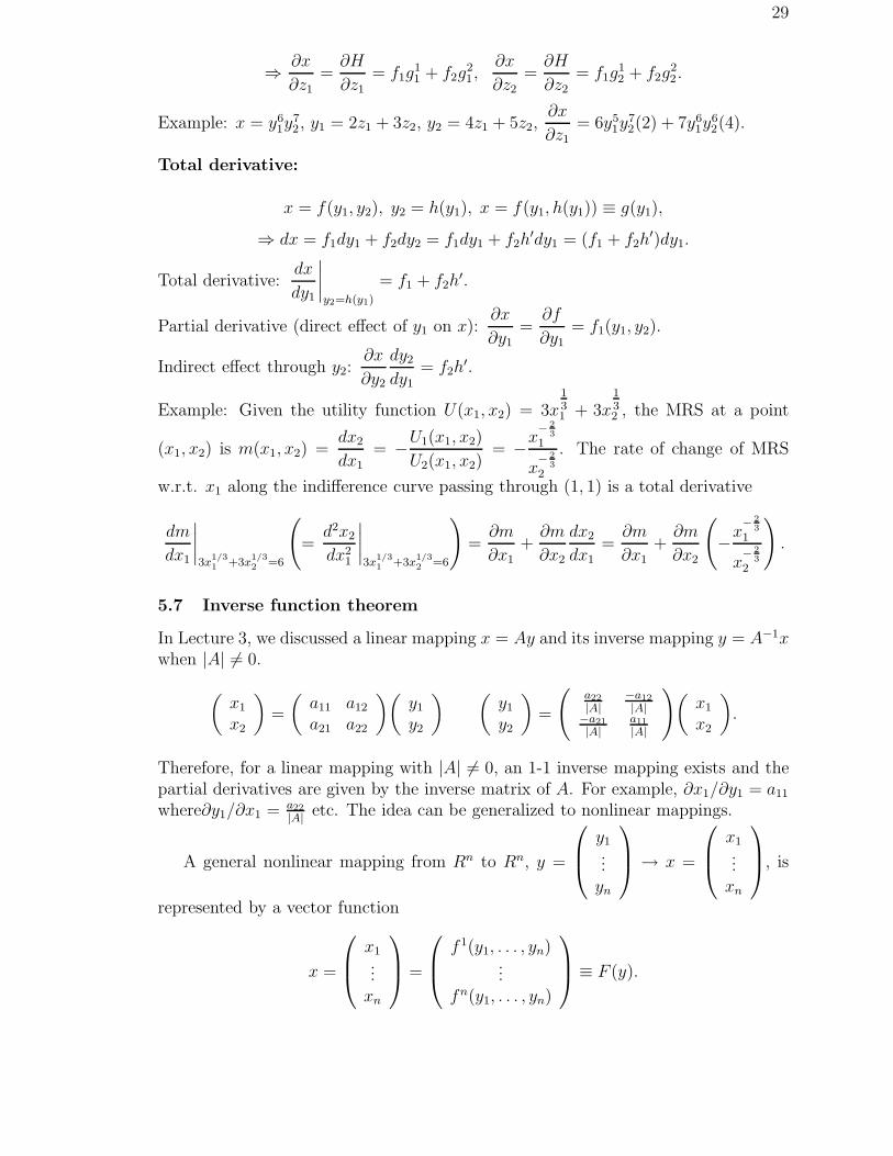
5.6 Concepts of total differentials and applications
Let x = f(y1, y2). Define ∆x ≡ f(y1 + ∆y1, y2 + ∆y2) − f(y1, y2), called the finitedifference of x.
∆x = f(y1 + ∆y1, y2 + ∆y2)− f(y1, y2)
= f(y1 + ∆y1, y2 + ∆y2)− f(y1, y2 + ∆y2) + f(y1, y2 + ∆y2)− f(y1, y2)
=f(y1 + ∆y1, y2 + ∆y2)− f(y1, y2 + ∆y2)
∆y1
∆y1 +f(y1, y2 + ∆y2)− f(y1, y2)
∆y2
∆y2
dx = f1(y1, y2)dy1 + f2(y1, y2)dy2.
dx, dy =
dy1...
dyn
: Infinitesimal changes of x (endogenous), y1, . . . , yn (exogenous).
Total differential of x = f(y1, . . . , yn):
dx = df = f1(y1, . . . , yn)dy1+. . .+fn(y1, . . . , yn)dyn = (f1, . . . , fn)
dy1...
dyn
= (∇f)′dy.
Implicit function rule:In many cases, the relationship between two variables are defined implicitly. Forexample, the indifference curve U(x1, x2) = U defines a relationship between x1 and
x2. To find the slope of the curvedx2
dx1, we use implicit function rule.
dU = U1(x1, x2)dx1 + U2(x1, x2)dx2 = dU = 0⇒;dx2
dx1= −U1(x1, x2)
U2(x1, x2).
Example: U(x1, x2) = 3x131 + 3x
132 = 6 defines an indifference curve passing through
the point (x1, x2) = (1, 1). The slope (Marginal Rate of Substitution) at (1, 1) can becalculated using implicit function rule.
dx2
dx1= −U1
U2= −x
− 2
3
1
x− 2
3
2
= −1
1= −1.
Multivariate chain rule:
x = f(y1, y2), y1 = g1(z1, z2), y2 = g2(z1, z2), ⇒ x = f(g1(z1, z2), g2(z1, z2)) ≡ H(z1, z2).
We can use the total differentials dx, dy1, dy2 to find the derivative∂x
∂z1
.
dx = (f1, f2)
(
dy1
dy2
)
= (f1, f2)
(
g11 g1
2
g21 g2
2
)(
dz1
dz2
)
= (f1g11+f2g
21, f1g
12+f2g
22)
(
dz1
dz2
)
.
29
⇒ ∂x
∂z1=
∂H
∂z1= f1g
11 + f2g
21,
∂x
∂z2=
∂H
∂z2= f1g
12 + f2g
22.
Example: x = y61y
72, y1 = 2z1 + 3z2, y2 = 4z1 + 5z2,
∂x
∂z1
= 6y51y
72(2) + 7y6
1y62(4).
Total derivative:
x = f(y1, y2), y2 = h(y1), x = f(y1, h(y1)) ≡ g(y1),
⇒ dx = f1dy1 + f2dy2 = f1dy1 + f2h′dy1 = (f1 + f2h
′)dy1.
Total derivative:dx
dy1
∣
∣
∣
∣
y2=h(y1)
= f1 + f2h′.
Partial derivative (direct effect of y1 on x):∂x
∂y1=
∂f
∂y1= f1(y1, y2).
Indirect effect through y2:∂x
∂y2
dy2
dy1
= f2h′.
Example: Given the utility function U(x1, x2) = 3x131 + 3x
132 , the MRS at a point
(x1, x2) is m(x1, x2) =dx2
dx1
= −U1(x1, x2)
U2(x1, x2)= −x
− 2
3
1
x− 2
3
2
. The rate of change of MRS
w.r.t. x1 along the indifference curve passing through (1, 1) is a total derivative
dm
dx1
∣
∣
∣
∣
3x1/3
1+3x
1/3
2=6
(
=d2x2
dx21
∣
∣
∣
∣
3x1/3
1+3x
1/3
2=6
)
=∂m
∂x1+
∂m
∂x2
dx2
dx1=
∂m
∂x1+
∂m
∂x2
(
−x− 2
3
1
x− 2
3
2
)
.
5.7 Inverse function theorem
In Lecture 3, we discussed a linear mapping x = Ay and its inverse mapping y = A−1xwhen |A| 6= 0.
(
x1
x2
)
=
(
a11 a12
a21 a22
)(
y1
y2
) (
y1
y2
)
=
(
a22
|A|−a12
|A|−a21
|A|a11
|A|
)
(
x1
x2
)
.
Therefore, for a linear mapping with |A| 6= 0, an 1-1 inverse mapping exists and thepartial derivatives are given by the inverse matrix of A. For example, ∂x1/∂y1 = a11
where∂y1/∂x1 = a22
|A| etc. The idea can be generalized to nonlinear mappings.
A general nonlinear mapping from Rn to Rn, y =
y1...
yn
→ x =
x1...
xn
, is
represented by a vector function
x =
x1...
xn
=
f 1(y1, . . . , yn)...
fn(y1, . . . , yn)
≡ F (y).
30
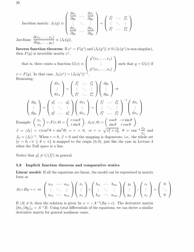
Jacobian matrix: JF (y) ≡
∂x1
∂y1. . .
∂x1
∂yn...
. . ....
∂xn
∂y1. . .
∂xn
∂yn
=
f 11 . . . f 1
n...
. . ....
fn1 . . . fn
n
.
Jacobian:∂(x1, . . . , xn)
∂(y1, . . . , yn)≡ |JF (y)|.
Inverse function theorem: If x∗ = F (y∗) and |JF (y∗)| 6= 0 (JF (y∗) is non-singular),then F (y) is invertible nearby x∗,
that is, there exists a function G(x) ≡
g1(x1, . . . , xn)...
gn(x1, . . . , xn)
such that y = G(x) if
x = F (y). In that case, JG(x∗) = (JF (y∗))−1.Reasoning:
dx1...
dxn
=
f 11 . . . f 1
n...
. . ....
fn1 . . . fn
n
dy1...
dyn
⇒
dy1...
dyn
=
g11 . . . g1
n...
. . ....
gn1 . . . gn
n
dx1...
dxn
=
f 11 . . . f 1
n...
. . ....
fn1 . . . fn
n
−1
dx1...
dxn
Example:
(
x1
x2
)
= F (r, θ) =
(
r cos θr sin θ
)
. JF (r, θ) =
(
cos θ −r sin θsin θ r cos θ
)
.
J = |JF | = r(cos2 θ + sin2 θ) = r > 0, ⇒ r =√
x21 + x2
2, θ = tan−1 x2
x1and
JG = (JF )−1. When r = 0, J = 0 and the mapping is degenerate, i.e., the whole set{r = 0,−π ≤ θ < π} is mapped to the origin (0, 0), just like the case in Lecture 3when the Null space is a line.
Notice that g11 6= 1/(f 1
1 ) in general.
5.8 Implicit function theorem and comparative statics
Linear model: If all the equations are linear, the model can be represtned in matrixform as
Ax+By = c ⇔
a11 · · · a1n...
. . ....
an1 · · · ann
x1...
xn
+
b11 · · · b1m...
. . ....
bn1 · · · anm
y1...
ym
−
c1...cn
=
0. . .
0
.
If |A| 6= 0, then the solution is given by x = −A−1(By + c). The derivative matrix[∂xi/∂yj]ij = A−1B. Using total differentials of the equations, we can derive a similarderivative matrix for general nonlinear cases.
31
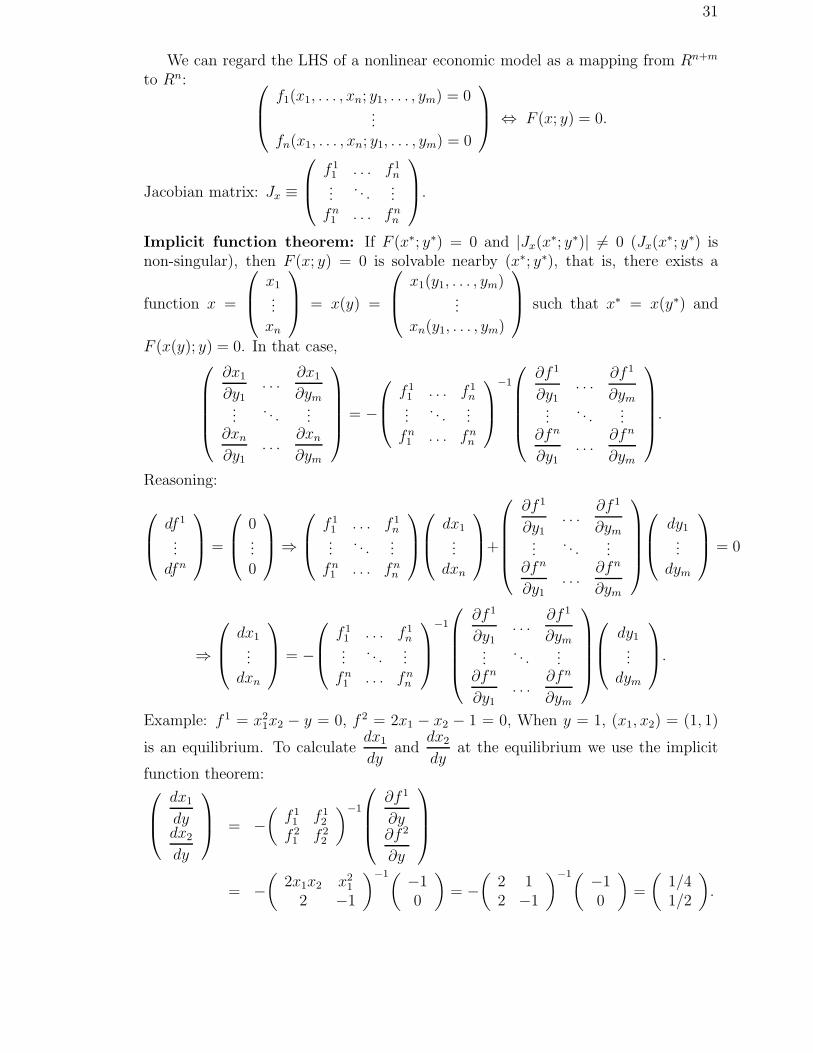
We can regard the LHS of a nonlinear economic model as a mapping from Rn+m
to Rn:
f1(x1, . . . , xn; y1, . . . , ym) = 0...
fn(x1, . . . , xn; y1, . . . , ym) = 0
⇔ F (x; y) = 0.
Jacobian matrix: Jx ≡
f 11 . . . f 1
n...
. . ....
fn1 . . . fn
n
.
Implicit function theorem: If F (x∗; y∗) = 0 and |Jx(x∗; y∗)| 6= 0 (Jx(x
∗; y∗) isnon-singular), then F (x; y) = 0 is solvable nearby (x∗; y∗), that is, there exists a
function x =
x1...
xn
= x(y) =
x1(y1, . . . , ym)...
xn(y1, . . . , ym)
such that x∗ = x(y∗) and
F (x(y); y) = 0. In that case,
∂x1
∂y1. . .
∂x1
∂ym...
. . ....
∂xn
∂y1
. . .∂xn
∂ym
= −
f 11 . . . f 1
n...
. . ....
fn1 . . . fn
n
−1
∂f 1
∂y1. . .
∂f 1
∂ym...
. . ....
∂fn
∂y1
. . .∂fn
∂ym
.
Reasoning:
df 1
...dfn
=
0...0
⇒
f 11 . . . f 1
n...
. . ....
fn1 . . . fn
n
dx1...
dxn
+
∂f 1
∂y1. . .
∂f 1
∂ym...
. . ....
∂fn
∂y1. . .
∂fn
∂ym
dy1...
dym
= 0
⇒
dx1...
dxn
= −
f 11 . . . f 1
n...
. . ....
fn1 . . . fn
n
−1
∂f 1
∂y1. . .
∂f 1
∂ym...
. . ....
∂fn
∂y1
. . .∂fn
∂ym
dy1...
dym
.
Example: f 1 = x21x2 − y = 0, f 2 = 2x1 − x2 − 1 = 0, When y = 1, (x1, x2) = (1, 1)
is an equilibrium. To calculatedx1
dyand
dx2
dyat the equilibrium we use the implicit
function theorem:
dx1
dydx2
dy
= −
(
f 11 f 1
2
f 21 f 2
2
)−1
∂f 1
∂y∂f 2
∂y
= −(
2x1x2 x21
2 −1
)−1( −10
)
= −(
2 12 −1
)−1( −10
)
=
(
1/41/2
)
.
32
5.9 Problems
1. Given the demand function Qd = (100/P )− 10, find the demand elasticity η.
2. Given Y = X21X2 + 2X1X
22 , find ∂Y/∂X1, ∂2Y/∂X2
1 , and ∂2Y/∂X1∂X2, andthe total differential DY .
3. Given Y = F (X1, X2)+f(X1)+g(X2), find ∂Y/∂X1, ∂2Y/∂X21 , and ∂2Y/∂X1∂X2.
4. Given the consumption function C = C(Y − T (Y )), find dC/dY .
5. Given that Q = D(q ∗ e/P ), find dQ/dP .
6. Y = X21X2, Z = Y 2 + 2Y − 2, use chain rule to derive ∂Z/∂X1 and ∂Z/∂X2.
7. Y1 = X1 +2X2, Y2 = 2X1 +X2, and Z = Y1Y2, use chain rule to derive ∂Z/∂X1
and ∂Z/∂X2.
8. Let U(X1, X2) = X1X22 + X2
1X2 and X2 = 2X1 + 1, find the partial derivative∂U/∂X1 and the total derivative dU/dX1.
9. X2 + Y 3 = 1, use implicit function rule to find dY/dX.
10. X21 + 2X2
2 + Y 2 = 1, use implicit function rule to derive ∂Y/∂X1 and ∂Y/∂X2.
11. F (Y1, Y2, X) = Y1 − Y2 + X − 1 = 0 and G(Y1, Y2, X) = Y 21 + Y 2
2 + X2 − 1 = 0.use implicit function theorem to derive dY1/dX and dY2/dX.
12. In a Cournot quantity competition duopoly model with heterogeneous products,the demand functions are given by
Q1 = a− P1 − cP2, Q2 = a− cP1 − P2; 1 ≥ c > 0.
(a) For what value of c can we invert the demand functions to obtain P1 andP2 as functions of Q1 and Q2?
(b) Calculate the inverse demand functions P1 = P1(Q1, Q2) and P2 = P2(Q1, Q2).
(c) Derive the total revenue functions TR1(Q1, Q2) = P1(Q1, Q2)Q1 and TR2(Q1, Q2) =P2(Q1, Q2)Q2.
13. In a 2-good market equilibrium model, the inverse demand functions are givenby
P1 = A1Qα−11 Qβ
2 , P2 = A2Qα1 Qβ−1
2 ; α, β > 0.
(a) Calculate the Jacobian matrix
(
∂P1/∂Q1 ∂P1/∂Q2
∂P2/∂Q1 ∂P2/∂Q2
)
and Jacobian∂(P1, P2)
∂(Q1, Q2).
What condition(s) should the parameters satisfy so that we can invert thefunctions to obtain the demand functions?
(b) Derive the Jacobian matrix of the derivatives of (Q1, Q2) with respect to
(P1, P2),
(
∂Q1/∂P1 ∂Q1/∂P2
∂Q2/∂P1 ∂Q2/∂P2
)
.
33
5.10 Proofs of important theorems of differentiation
Rolle’s theorem: If f(x) ∈ C[a, b], f ′(x) exists for all x ∈ (a, b), and f(a) = f(b) =0, then there exists a c ∈ (a, b) such that f ′(c) = 0.Proof:Case 1: f(x) ≡ 0 ∀x ∈ [a, b]⇒ f ′(x) = 0 ∀x ∈ (a, b)./Case 2: f(x) 6≡ 0 ∈ [a, b] ⇒ ∃e, c such that f(e) = m ≤ f(x) ≤ M = f(c) andM > m. Assume that M 6= 0 (otherwise m 6= 0 and the proof is similar). It is easyto see that f ′
−(c) ≥ 0 and f ′+(c) ≤ 0. Therefore, f ′(c) = 0. Q.E.D.
Mean Value theorem: If f(x) ∈ C[a, b] and f ′(x) exists for all x ∈ (a, b). Thenthere exists a c ∈ (a, b) such that
f(b)− f(a) = f ′(c)(b− a).
Proof:Consider the function
φ(x) ≡ f(x)−[
f(a) +f(b)− f(a)
b− a(x− a)
]
.
It is clear that φ(x) ∈ C[a, b] and φ′(x) exists for all x ∈ (a, b). Also, φ(a) = φ(b) = 0so that the conditions of Rolle’s Theorem are satisfied for φ(x). Hence, there existsa c ∈ (a, b) such that φ′(c) = 0, or
φ′(c) = f ′(c)− f(b)− f(a)
b− a= 0 ⇒ f ′(c) =
f(b)− f(a)
b− a= 0.
Q.E.D.
Taylor’s Theorem: If f(x) ∈ Cr[a, b] and f (r+1)(x) exists for all x ∈ (a, b). Thenthere exists a c ∈ (a, b) such that
f(b) = f(a)+f ′(a)(b−a)+1
2f ′′(a)(b−a)2+. . .+
1
r!f (r)(a)(b−a)r+
1
(r + 1)!f (r+1)(c)(b−a)r+1.
Proof:Define ξ ∈ R
(b− a)r+1
(r + 1)!ξ ≡ f(b)−
[
f(a) + f ′(a)(b− a) +1
2f ′′(a)(b− a)2 + . . . +
1
r!f (r)(a)(b− a)r
]
.
Consider the function
φ(x) ≡ f(b)−[
f(x) + f ′(x)(b− x) +1
2f ′′(x)(b− x)2 + . . . +
1
r!f (r)(x)(b− x)r +
ξ
(r + 1)!(b− x)r+1
]
.

34
It is clear that φ(x) ∈ C[a, b] and φ′(x) exists for all x ∈ (a, b). Also, φ(a) = φ(b) = 0so that the conditions of Rolle’s Theorem are satisfied for φ(x). Hence, there existsa c ∈ (a, b) such that φ′(c) = 0, or
φ′(c) =ξ − f (r+1)(c)
r!= 0 ⇒ f (r+1)(c) = ξ.
Q.E.D.
Inverse Function Theorem: Let E ⊆ Rn be an open set. Suppose f : E → Rn
is C1(E), a ∈ E, f(a) = b, and A = J(f(a)), |A| 6= 0. Then there exist open setsU, V ⊂ Rn such that a ∈ U , b ∈ V , f is one to one on U , f(U) = V , and f−1 : V → Uis C1(U).Proof:(1. Find U .) Choose λ ≡ |A|/2. Since f ∈ C1(E), there exists a neighborhood U ⊆ Ewith a ∈ U such that ‖J(f(x))−A‖ < λ.(2. Show that f(x) is one to one in U .) For each y ∈ Rn define φy on E byφy(x) ≡ x + A−1(y − f(x)). Notice that f(x) = y if and only if x is a fixed point of
φy. Since J(φy(x)) = I − A−1J(f(x)) = A−1[A− J(f(x))]⇒ ‖J(φy(x))‖ <1
2on U .
Therefore φy(x) is a contraction mapping and there exists at most one fixed point inU . Therefore, f is one to one in U .(3. V = f(U) is open so that f−1 is continuous.) Let V = f(U) and y0 = f(x0) ∈ Vfor x0 ∈ U . Choose an open ball B about x0 with radius ρ such that the closure[B] ⊆ U . To prove that V is open, it is enough to show that y ∈ V whenever‖y − y0‖ < λρ. So fix y such that ‖y − y0‖ < λρ. With φy defined above,
‖φy(x0)− x0‖ = ‖A−1(y − y0)‖ < ‖A−1‖λρ =ρ
2.
If x ∈ [B] ⊆ U , then
‖φy(x)− x0‖ ≤ ‖φy(x)− φy(x0)‖+ ‖φy(x0)− x0‖ <1
2‖x− x0‖+
ρ
2≤ ρ.
That is, φy(x) ∈ [B]. Thus, φy(x) is a contraction of the complete space [B] into itself.Hence, φy(x) has a unique fixed point x ∈ [B] and y = f(x) ∈ f([B]) ⊂ f(U) = V .(4. f−1 ∈ C−1.) Choose y1, y2 ∈ V , there exist x1, x2 ∈ U such that f(x1) = y1,f(x2) = y2.
φy(x2)− φy(x1) = x2 − x1 + A−1(f(x1)− f(x2)) = (x2 − x1)−A−1(y2 − y1).
⇒ ‖(x2−x1)−A−1(y2−y1)‖ ≤1
2‖x2−x1‖ ⇒
1
2‖x2−x1‖ ≤ ‖A−1(y2−y1)‖ ≤
1
2λ‖y2−y1‖
or ‖x2 − x1‖ ≤1
λ‖y2 − y1‖. It follows that (f ′)−1 exists locally about a. Since
f−1(y2)− f−1(y1)− (f ′)−1(y1)(y2 − y1) = (x2 − x1)− (f ′)−1(y1)(y2 − y1)
= −(f ′)−1(y1)[−f ′(x1)(x2 − x1) + f(x2)− f(x1)],
35
We have
‖f−1(y2)− f−1(y1)− (f ′)−1(y1)(y2 − y1)‖‖y2 − y1‖
≤ ‖(f′)−1‖λ
‖f(x2)− f(x1)− f ′(x1)(x2 − x1)‖‖x2 − x1‖
.
As y2→y1, x2→x1. Hence (f 1−)′(y) = {f ′[f−1(y)]} for y ∈ V . Since f−1 is differ-entiable, it is continuous. Also, f ′ is continuous and its inversion, where it exists, iscontinuous. Therefore (f−1)′ is continuous or f−1 ∈ C1(V ). Q.E.D.
Implicit Function Theorem: Let E ⊆ R(n+m) be an open set and a ∈ Rn, b ∈ Rm,(a, b) ∈ E. Suppose f : E → Rn is C1(E) and f(a, b) = 0, and J(f(a, b)) 6= 0. Thenthere exist open sets A ⊂ Rn and B ⊂ Rm a ∈ A and b ∈ B, such that for eachx ∈ B, there exists a unique g(x) ∈ A such that f(g(x), x) = 0 and g : B → A isC1(B).Proof:Defining F : Rn+m→Rn+m by F (x, y) ≡ (x, f(x, y)). Note that since
J(F (a, b)) =
(
∂xi
∂xj
)
1≤i,j≤n
(
∂xi
∂xn+j
)
1≤i≤n,1≤j≤m(
∂fi
∂xj
)
1≤i≤m,1≤j≤n
(
∂fi
∂xn+j
)
1≤i,j≤m
=
(
I ON M
)
,
|J(F (a, b))| = |M | 6= 0. By the Inverse Function Theorem there exists an open setV ⊆ Rn+m containing F (a, b) = (a, 0) and an open set of the form A × B ⊆ Econtaining (a, b), such that F : A × B→V has a C1 inverse F−1 : V→A × B. F−1
is of the form F−1(x, y) = (x, φ(x, y)) for some C1 function φ. Define the projectionπ : Rn+m→Rm by π(x, y) = y. Then π ◦ F (x, y) = f(x, y). Therefore
f(x, φ(x, y)) = f ◦F−1(x, y) = (π ◦F ) ◦F−1(x, y) = π ◦ (F ◦F−1)(x, y) = π(x, y) = y
and f(x, φ(x, 0)) = 0. So, define g : A→B by g(x) = φ(x, 0). Q.E.D.
36
6 Comparative Statics – Economic applications
6.1 Partial equilibrium model
Q = D(P, Y )∂D
∂P< 0,
∂D
∂Y> 0 end. var: Q, P.
Q = S(P ) S ′(P ) > 0 ex. var: Y..
f 1(P, Q; Y ) = Q−D(P, Y ) = 0df 1
dY=
dQ
dY− ∂D
∂P
dP
dY− ∂D
∂Y= 0
f 2(P, Q; Y ) = Q− S(P ) = 0df 2
dY=
dQ
dY− S ′(P )
dP
dY= 0
.
(
1 −∂D
∂P1 −S ′(P )
)
dQ
dYdP
dY
=
(
∂D
∂Y0
)
, |J | =∣
∣
∣
∣
∣
1 −∂D
∂P1 −S ′(P )
∣
∣
∣
∣
∣
= −S ′(P ) +∂D
∂P< 0.
dQ
dY=
∣
∣
∣
∣
∣
∂D
∂Y−∂D
∂P0 −S ′(P )
∣
∣
∣
∣
∣
|J | =−∂D
∂YS ′(P )
|J | > 0,dP
dY=
∣
∣
∣
∣
∣
1∂D
∂Y1 0
∣
∣
∣
∣
∣
|J | =−∂D
∂Y|J | > 0.
6.2 Income determination model
C = C(Y ) 0 < C ′(Y ) < 1.I = I(r) I ′(r) < 0 end. var. C, Y, IY = C + I + G ex. var. G, r.
Y = C(Y ) + I(r) + G⇒ dY = C ′(Y )dY + I ′(r)dr + dG⇒ dY =I ′(r)dr + dG
1− C ′(Y ).
∂Y
∂r=
I ′(r)
1− C ′(Y )< 0,
∂Y
∂G=
1
1− C ′(Y )> 0.
6.2.1 Income determination and trade
Consider an income determination model with import and export:
C = C(Y ) 1 > Cy > 0, I = I ,
M = M(Y, e) My > 0, Me < 0 X = X(Y ∗, e), Xy∗ > 0, Xe > 0
C + I + X −M = Y,
where import M is a function of domestic income and exchange rate e and exportX is a function of exchange rate and foreign income Y ∗, both are assumed here asexogenous variables. Substituting consumption, import, and export functions intothe equilibrium condition, we have
C(Y )+I+X(Y ∗, e)−M(Y, e) = Y, ⇒F (Y, e, Y ∗) ≡ C(Y )+I+X(Y ∗, e)−M(Y, e)−Y = 0..
37
Use implicit function rule to derive∂Y
∂Iand determine its sign:
∂Y
∂I= −FI
Fy
=1
1− C ′(Y ) + My
.
Use implicit function rule to derive∂Y
∂eand determine its sign:
∂Y
∂e= −Fe
Fy=
Xe −Me
1− C ′(Y ) + My.
Use implicit function rule to derive∂Y
∂Y ∗ and determine its sign:
∂Y
∂Y ∗ = −Fy∗
Fy=
Xy∗
1− C ′(Y ) + My.
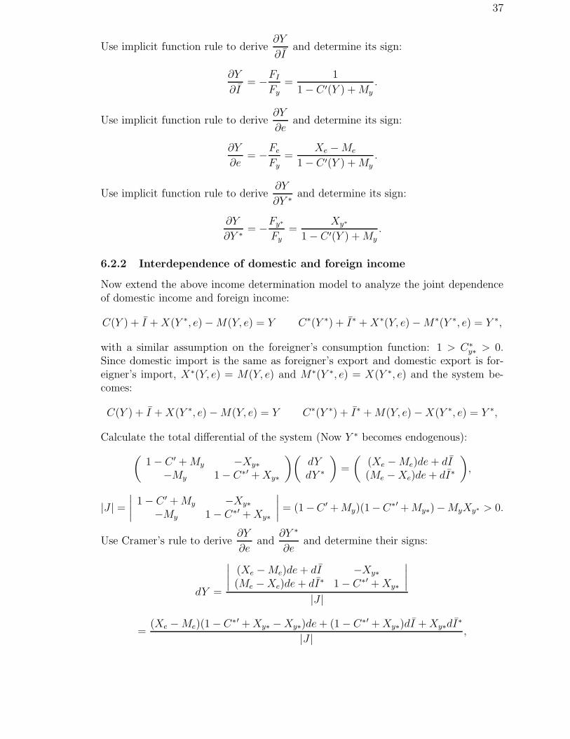
6.2.2 Interdependence of domestic and foreign income
Now extend the above income determination model to analyze the joint dependenceof domestic income and foreign income:
C(Y ) + I + X(Y ∗, e)−M(Y, e) = Y C∗(Y ∗) + I∗ + X∗(Y, e)−M∗(Y ∗, e) = Y ∗,
with a similar assumption on the foreigner’s consumption function: 1 > C∗y∗ > 0.
Since domestic import is the same as foreigner’s export and domestic export is for-eigner’s import, X∗(Y, e) = M(Y, e) and M∗(Y ∗, e) = X(Y ∗, e) and the system be-comes:
C(Y ) + I + X(Y ∗, e)−M(Y, e) = Y C∗(Y ∗) + I∗ + M(Y, e)−X(Y ∗, e) = Y ∗,
Calculate the total differential of the system (Now Y ∗ becomes endogenous):
(
1− C ′ + My −Xy∗−My 1− C∗′ + Xy∗
)(
dYdY ∗
)
=
(
(Xe −Me)de + dI(Me −Xe)de + dI∗
)
,
|J | =∣
∣
∣
∣
1− C ′ + My −Xy∗−My 1− C∗′ + Xy∗
∣
∣
∣
∣
= (1−C ′ + My)(1−C∗′ + My∗)−MyXy∗ > 0.
Use Cramer’s rule to derive∂Y
∂eand
∂Y ∗
∂eand determine their signs:
dY =
∣
∣
∣
∣
(Xe −Me)de + dI −Xy∗(Me −Xe)de + dI∗ 1− C∗′ + Xy∗
∣
∣
∣
∣
|J |
=(Xe −Me)(1− C∗′ + Xy∗ −Xy∗)de + (1− C∗′ + Xy∗)dI + Xy∗dI∗
|J | ,

38
dY ∗ =
∣
∣
∣
∣
1− C ′ + My (Xe −Me)de + dI−My (Me −Xe)de + dI∗
∣
∣
∣
∣
|J |
=−(Xe −Me)(1− C ′ + My −My)de + (1− C ′ + My)dI∗ + XydI
|J | .
∂Y
∂e=
(Xe −Me)(1− C∗′)
|J | > 0,∂Y ∗
∂e=−(Xe −Me)(1− C ′)
|J | < 0.
Derive∂Y
∂Iand
∂Y ∗
∂Iand determine their signs:
∂Y
∂I= −1− C∗′ + My∗
|J | > 0,∂Y ∗
∂I=
My
|J | < 0.
6.3 IS-LM model
C = C(Y ) 0 < C ′(Y ) < 1 Md = L(Y, r)∂L
∂Y> 0,
∂L
∂r< 0
I = I(r) I ′(r) < 0 Ms = MY = C + I + G Md = Ms.
end. var: Y , C, I, r, Md, Ms. ex. var: G, M .
Y − C(Y )− I(r) = GL(Y, r) = M
⇒(1− C ′(Y ))dY − I ′(r)dr = dG
∂L
∂YdY +
∂L
∂rdr = dM
(
1− C ′ −I ′
LY Lr
)(
dYdr
)
=
(
dGdM
)
, |J | =∣
∣
∣
∣
1− C ′ −I ′
LY Lr
∣
∣
∣
∣
= (1−C ′)Lr+I ′LY < 0.
dY =
∣
∣
∣
∣
dG −I ′
dM Lr
∣
∣
∣
∣
|J | =LrdG + I ′dM
|J | , dr =
∣
∣
∣
∣
1− C ′ dGLY dM
∣
∣
∣
∣
|J | =−LY dG + (1− C ′)dM
|J |∂Y
∂G=
Lr
|J | > 0,∂Y
∂M=
I ′
|J | > 0,∂r
∂G= −LY
|J | > 0,∂r
∂M=
(1− C ′)
|J | < 0.
6.4 Two-market general equilibrium model
Q1d = D1(P1, P2) D11 < 0, Q2d = D2(P1, P2) D2
2 < 0, D21 > 0.
Q1s = S1 Q2s = S2(P2) S ′2(P2) > 0
Q1d = Q1s Q2d = Q2s
end. var: Q1, Q2, P1, P2. ex. var: S1.
D1(P1, P2) = S1 ⇒ D11dP1 + D1
2dP2 = dS1
D2(P1, P2)− S2(P2) = 0 D21dP1 + D2
2dP2 − S ′2dP2 = 0.
39
(
D11 D1
2
D21 D2
2 − S ′2
)(
dP1
dP2
)
=
(
dS1
0
)
, |J | =∣
∣
∣
∣
D11 D1
2
D21 D2
2 − S ′2
∣
∣
∣
∣
= D11(D
22−S ′
2)−D12D
21.
Assumption: |D11| > |D1
2| and |D22| > |D2
1| (own-effects dominate), ⇒ |J | > 0.
dP1
dS1
=D2
2 − S ′2
|J | < 0,dP2
dS1
=−D2
1
|J | < 0
From Q1s = S1,∂Q1
∂S1
= 1. To calculate∂Q2
∂S1
, we have to use chain rule:
∂Q2
∂S1
= S ′2
dP2
dS1
< 0.
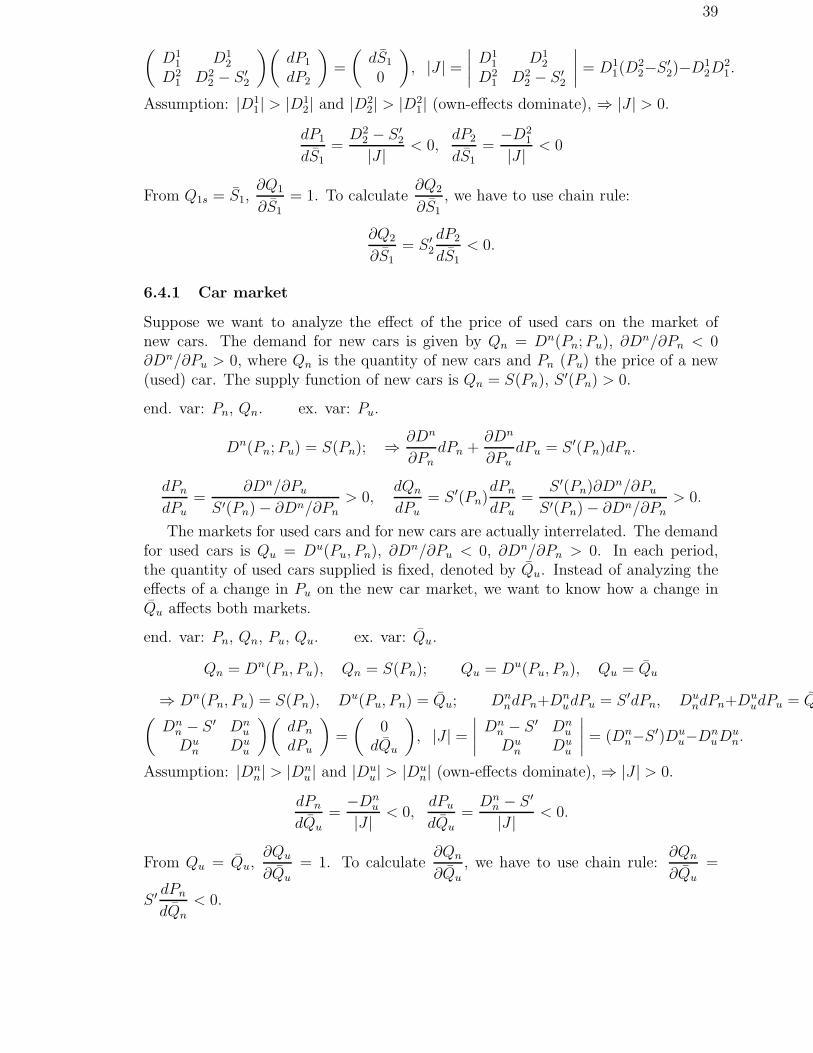
6.4.1 Car market
Suppose we want to analyze the effect of the price of used cars on the market ofnew cars. The demand for new cars is given by Qn = Dn(Pn; Pu), ∂Dn/∂Pn < 0∂Dn/∂Pu > 0, where Qn is the quantity of new cars and Pn (Pu) the price of a new(used) car. The supply function of new cars is Qn = S(Pn), S ′(Pn) > 0.
end. var: Pn, Qn. ex. var: Pu.
Dn(Pn; Pu) = S(Pn); ⇒ ∂Dn
∂PndPn +
∂Dn
∂PudPu = S ′(Pn)dPn.
dPn
dPu=
∂Dn/∂Pu
S ′(Pn)− ∂Dn/∂Pn> 0,
dQn
dPu= S ′(Pn)
dPn
dPu=
S ′(Pn)∂Dn/∂Pu
S ′(Pn)− ∂Dn/∂Pn> 0.
The markets for used cars and for new cars are actually interrelated. The demandfor used cars is Qu = Du(Pu, Pn), ∂Dn/∂Pu < 0, ∂Dn/∂Pn > 0. In each period,the quantity of used cars supplied is fixed, denoted by Qu. Instead of analyzing theeffects of a change in Pu on the new car market, we want to know how a change inQu affects both markets.
end. var: Pn, Qn, Pu, Qu. ex. var: Qu.
Qn = Dn(Pn, Pu), Qn = S(Pn); Qu = Du(Pu, Pn), Qu = Qu
⇒ Dn(Pn, Pu) = S(Pn), Du(Pu, Pn) = Qu; DnndPn+Dn
udPu = S ′dPn, DundPn+Du
udPu = Q(
Dnn − S ′ Dn
u
Dun Du
u
)(
dPn
dPu
)
=
(
0dQu
)
, |J | =∣
∣
∣
∣
Dnn − S ′ Dn
u
Dun Du
u
∣
∣
∣
∣
= (Dnn−S ′)Du
u−DnuDu
n.
Assumption: |Dnn| > |Dn
u | and |Duu| > |Du
n| (own-effects dominate), ⇒ |J | > 0.
dPn
dQu
=−Dn
u
|J | < 0,dPu
dQu
=Dn
n − S ′
|J | < 0.
From Qu = Qu,∂Qu
∂Qu
= 1. To calculate∂Qn
∂Qu
, we have to use chain rule:∂Qn
∂Qu
=
S ′ dPn
dQn
< 0.

40
6.5 Classic labor market model
L = h(w) h′ > 0 labor supply function
w = MPPL =∂Q
∂L= FL(K, L) FLK > 0, FLL < 0 labor demand function.
endogenous variables: L, w. exogenous variable: K.
L− h(w) = 0 ⇒ dL− h′(w)dw = 0w − FL = 0 dw − FLLdL− FLKdK = 0
.
(
1 −h′(w)−FLL 1
)(
dLdw
)
=
(
0FLKdK
)
, |J | =∣
∣
∣
∣
1 −h′(w)−FLL 1
∣
∣
∣
∣
= 1−h′(w)FLL > 0.
dL
dK=
∣
∣
∣
∣
0 −h′(w)FLK 1
∣
∣
∣
∣
|J | =h′FLK
|J | > 0,dw
dK=
∣
∣
∣
∣
1 0−FLL FLK
∣
∣
∣
∣
|J | =FLK
|J | > 0.
6.6 Problem
1. Let the demand and supply functions for a commodity be
Q = D(P ) D′(P ) < 0Q = S(P, t) ∂S/∂P > 0, ∂S/∂t < 0,
where t is the tax rate on the commodity.(a) Derive the total differentail of each equation.(b) Use Cramer’s rule to compute dQ/dt and dP/dt.(c) Determine the sign of dQ/dt and dP/dt.(d) Use the Q− P diagram to explain your results.
2. Suppose consumption C depends on total wealth W , which is predetermind, aswell as on income Y . The IS-LM model becomes
C = C(Y, W ) 0 < CY < 1 CW > 0 MS = MI = I(r) I ′(r) < 0 Y = C + IMD = L(Y, r) LY > 0 Lr < 0 MS = MD
(a) Which variables are endogenous? Which are exogenous?(b) Which equations are behavioral/institutional, which are equilibrium condi-tions?
The model can be reduced to
Y − C(Y, W )− I(r) = 0, L(Y, r) = M.
(c) Derive the total differential for each of the two equations.(d) Use Cramer’s rule to derive the effects of an increase in W on Y and r, ie.,derive ∂Y/∂W and ∂r/∂W .(e) Determine the signs of ∂Y/∂W and ∂r/∂W .
41
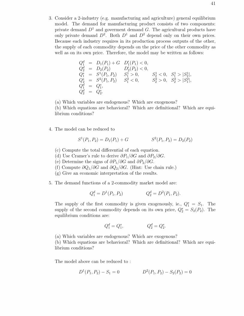
3. Consider a 2-industry (e.g. manufacturing and agriculture) general equilibriummodel. The demand for manufacturing product consists of two components:private demand D1 and goverment demand G. The agricultural products haveonly private demand D2. Both D1 and D2 depend only on their own prices.Because each industry requires in its production process outputs of the other,the supply of each commodity depends on the price of the other commodity aswell as on its own price. Therefore, the model may be written as follows:
Qd1 = D1(P1) + G D′
1(P1) < 0,Qd
2 = D2(P2) D′2(P2) < 0,
Qs1 = S1(P1, P2) S1
1 > 0, S12 < 0, S1
1 > |S12 |,
Qs2 = S2(P1, P2) S2
1 < 0, S22 > 0, S2
2 > |S21 |,
Qd1 = Qs
1,Qd
2 = Qs2.
(a) Which variables are endogenous? Which are exogenous?(b) Which equations are behavioral? Which are definitional? Which are equi-librium conditions?
4. The model can be reduced to
S1(P1, P2) = D1(P1) + G S2(P1, P2) = D2(P2)
(c) Compute the total differential of each equation.(d) Use Cramer’s rule to derive ∂P1/∂G and ∂P2/∂G.(e) Determine the signs of ∂P1/∂G and ∂P2/∂G.(f) Compute ∂Q1/∂G and ∂Q2/∂G. (Hint: Use chain rule.)(g) Give an economic interpretation of the results.
5. The demand functions of a 2-commodity market model are:
Qd1 = D1(P1, P2) Qd
2 = D2(P1, P2).
The supply of the first commodity is given exogenously, ie., Qs1 = S1. The
supply of the second commodity depends on its own price, Qs2 = S2(P2). The
equilibrium conditions are:
Qd1 = Qs
1, Qd2 = Qs
2.
(a) Which variables are endogenous? Which are exogenous?(b) Which equations are behavioral? Which are definitional? Which are equi-librium conditions?
The model above can be reduced to :
D1(P1, P2)− S1 = 0 D2(P1, P2)− S2(P2) = 0

42
Suppose that both commodities are not Giffen good (hence, Dii < 0, i = 1, 2),
that each one is a gross substitute for the other (ie., Dij > 0, i 6= j), that
|Dii| > |Di
j |, and that S ′2(P2) > 0.
(c) Calculate the total differential of each equation of the reduced model.(d) Use Cramer’s rule to derive ∂P1/∂S1 and ∂P2/∂S1.(e) Determine the signs of ∂P1/∂S1 and ∂P2/∂S1.(f) Compute ∂Q1/∂S1 and ∂Q2/∂S1 and determine their signs.
6. The demand functions for fish and chicken are as follows:
QdF = DF (PF − PC), D′
F < 0
QdC = DC(PC − PF ), D′
C < 0
where PF , PC are price of fish and price of chicken respectively. The supplyof fish depends on the number of fishermen (N) as well as its price PF : Qs
F =F (PF , N), FPF
> 0, FN > 0. The supply of chicken depends only on its pricePC : Qs
C = C(PC), C ′ > 0. The model can be reduced to
DF (PF − PC) = F (PF , N)DC(PC − PF ) = C(PC)
(a) Find the total differential of the reduced system.(b) Use Cramer’s rule to find dPF/dN and dPC/dN .(c) Determine the signs of dPF /dN and dPC/dN . What is the economic mean-ing of your results?(d) Find dQC/dN .
7. In a 2-good market equilibrium model, the inverse demand functions are givenby
P1 = U1(Q1, Q2), P2 = U2(Q1, Q2);
where U1(Q1, Q2) and U2(Q1, Q2) are the partial derivatives of a utility functionU(Q1, Q2) with respect to Q1 and Q2, respectively.
(a) Calculate the Jacobian matrix
(
∂P1/∂Q1 ∂P1/∂Q2
∂P2/∂Q1 ∂P2/∂Q2
)
and Jacobian∂(P1, P2)
∂(Q1, Q2).
What condition(s) should the parameters satisfy so that we can invert thefunctions to obtain the demand functions?
(b) Derive the Jacobian matrix of the derivatives of (Q1, Q2) with respect to
(P1, P2),
(
∂Q1/∂P1 ∂Q1/∂P2
∂Q2/∂P1 ∂Q2/∂P2
)
.
(c) Suppose that the supply functions are
Q1 = a−1P1, Q2 = P2,
and Q∗1 and Q∗
2 are market equilibrium quantities. Find the comparative
staticsdQ∗
1
daand
dQ∗2
da. (Hint: Eliminate P1 and P2.)
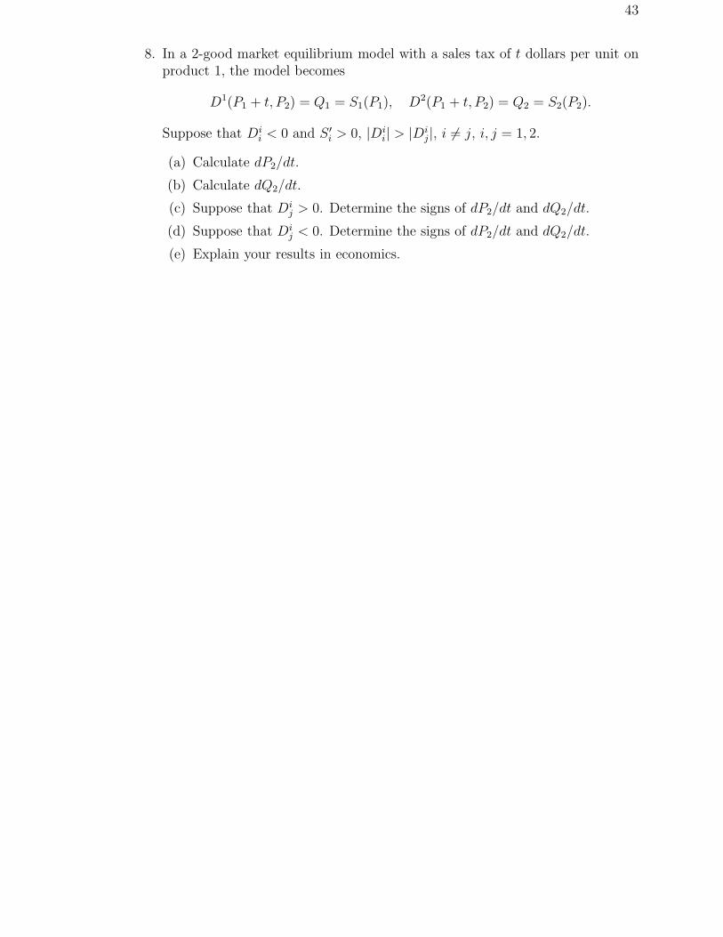
43
8. In a 2-good market equilibrium model with a sales tax of t dollars per unit onproduct 1, the model becomes
D1(P1 + t, P2) = Q1 = S1(P1), D2(P1 + t, P2) = Q2 = S2(P2).
Suppose that Dii < 0 and S ′
i > 0, |Dii| > |Di
j|, i 6= j, i, j = 1, 2.
(a) Calculate dP2/dt.
(b) Calculate dQ2/dt.
(c) Suppose that Dij > 0. Determine the signs of dP2/dt and dQ2/dt.
(d) Suppose that Dij < 0. Determine the signs of dP2/dt and dQ2/dt.
(e) Explain your results in economics.
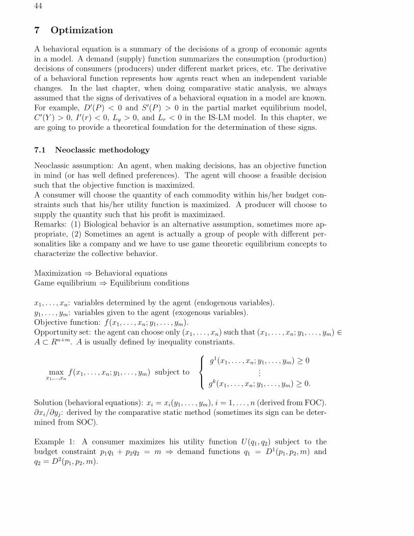
44
7 Optimization
A behavioral equation is a summary of the decisions of a group of economic agentsin a model. A demand (supply) function summarizes the consumption (production)decisions of consumers (producers) under different market prices, etc. The derivativeof a behavioral function represents how agents react when an independent variablechanges. In the last chapter, when doing comparative static analysis, we alwaysassumed that the signs of derivatives of a behavioral equation in a model are known.For example, D′(P ) < 0 and S ′(P ) > 0 in the partial market equilibrium model,C ′(Y ) > 0, I ′(r) < 0, Ly > 0, and Lr < 0 in the IS-LM model. In this chapter, weare going to provide a theoretical foundation for the determination of these signs.
7.1 Neoclassic methodology
Neoclassic assumption: An agent, when making decisions, has an objective functionin mind (or has well defined preferences). The agent will choose a feasible decisionsuch that the objective function is maximized.A consumer will choose the quantity of each commodity within his/her budget con-straints such that his/her utility function is maximized. A producer will choose tosupply the quantity such that his profit is maximizaed.Remarks: (1) Biological behavior is an alternative assumption, sometimes more ap-propriate, (2) Sometimes an agent is actually a group of people with different per-sonalities like a company and we have to use game theoretic equilibrium concepts tocharacterize the collective behavior.
Maximization ⇒ Behavioral equationsGame equilibrium ⇒ Equilibrium conditions
x1, . . . , xn: variables determined by the agent (endogenous variables).y1, . . . , ym: variables given to the agent (exogenous variables).Objective function: f(x1, . . . , xn; y1, . . . , ym).Opportunity set: the agent can choose only (x1, . . . , xn) such that (x1, . . . , xn; y1, . . . , ym) ∈A ⊂ Rn+m. A is usually defined by inequality constriants.
maxx1,...,xn
f(x1, . . . , xn; y1, . . . , ym) subject to
g1(x1, . . . , xn; y1, . . . , ym) ≥ 0...
gk(x1, . . . , xn; y1, . . . , ym) ≥ 0.
Solution (behavioral equations): xi = xi(y1, . . . , ym), i = 1, . . . , n (derived from FOC).∂xi/∂yj: derived by the comparative static method (sometimes its sign can be deter-mined from SOC).
Example 1: A consumer maximizes his utility function U(q1, q2) subject to thebudget constraint p1q1 + p2q2 = m ⇒ demand functions q1 = D1(p1, p2, m) andq2 = D2(p1, p2, m).
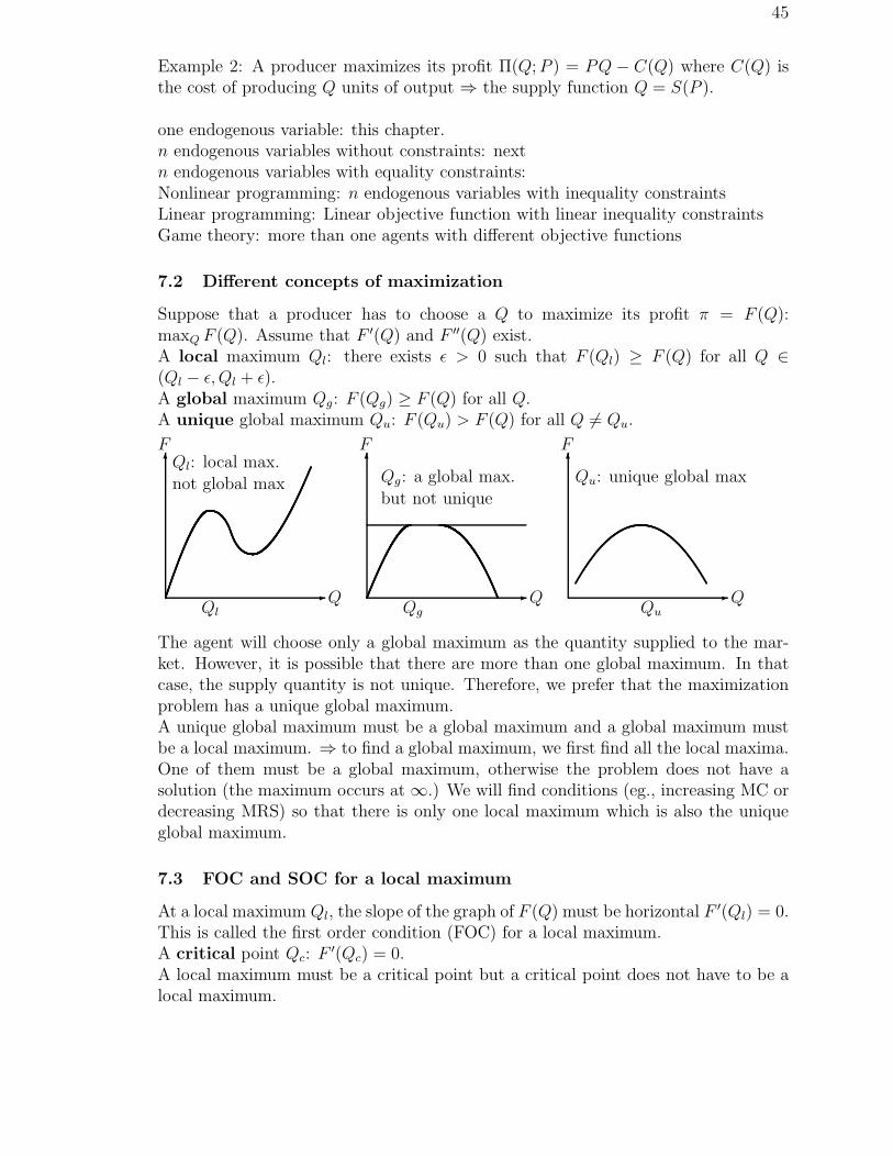
45
Example 2: A producer maximizes its profit Π(Q; P ) = PQ − C(Q) where C(Q) isthe cost of producing Q units of output ⇒ the supply function Q = S(P ).
one endogenous variable: this chapter.n endogenous variables without constraints: nextn endogenous variables with equality constraints:Nonlinear programming: n endogenous variables with inequality constraintsLinear programming: Linear objective function with linear inequality constraintsGame theory: more than one agents with different objective functions
7.2 Different concepts of maximization
Suppose that a producer has to choose a Q to maximize its profit π = F (Q):maxQ F (Q). Assume that F ′(Q) and F ′′(Q) exist.A local maximum Ql: there exists ǫ > 0 such that F (Ql) ≥ F (Q) for all Q ∈(Ql − ǫ, Ql + ǫ).A global maximum Qg: F (Qg) ≥ F (Q) for all Q.A unique global maximum Qu: F (Qu) > F (Q) for all Q 6= Qu.
-Q
6F
Ql
Ql: local max.not global max
- Q
6F
Qg: a global max.
but not unique
Qg
- Q
6F
Qu: unique global max
Qu
The agent will choose only a global maximum as the quantity supplied to the mar-ket. However, it is possible that there are more than one global maximum. In thatcase, the supply quantity is not unique. Therefore, we prefer that the maximizationproblem has a unique global maximum.A unique global maximum must be a global maximum and a global maximum mustbe a local maximum. ⇒ to find a global maximum, we first find all the local maxima.One of them must be a global maximum, otherwise the problem does not have asolution (the maximum occurs at∞.) We will find conditions (eg., increasing MC ordecreasing MRS) so that there is only one local maximum which is also the uniqueglobal maximum.
7.3 FOC and SOC for a local maximum
At a local maximum Ql, the slope of the graph of F (Q) must be horizontal F ′(Ql) = 0.This is called the first order condition (FOC) for a local maximum.A critical point Qc: F ′(Qc) = 0.A local maximum must be a critical point but a critical point does not have to be alocal maximum.

46
-Q
6F
F ′′(Qc) < 0
local max.
Qc
- Q
6F
F ′′(Qc) > 0
local min.
Qc
- Q
6F
F ′′(Qc) = 0
degenerate
Qc
A degenerate critical point: F ′(Q) = F ′′(Q) = 0.A non-degenerate critical point: F ′(Q) = 0, F ′′(Q) 6= 0.A non-degenerate critical point is a local maximum (minimum) if F ′′(Q) < 0 (F ′′(Q) >0).
FOC: F ′(Ql) = 0 SOC: F ′′(Ql) < 0
Example: F (Q) = −15Q+9Q2−Q3, F ′(Q) = −15+18Q−3Q2 = −3(Q−1)(Q−5).There are two critical points: Q = 1, 5. F ′′(Q) = 18 − 6Q, F ′′(1) = 12 > 0, andF ′′(5) = −12 < 0. Therefore, Q = 5 is a local maximum. It is a global maximum for0 ≤ Q <∞.
Remark 1 (Degeneracy): For a degenerate critical point, we have to check higherorder derivatives. If the lowest order non-zero derivative is of odd order, then it is areflect point; eg., F (Q) = (Q−5)3, F ′(5) = F ′′(5) = 0 and F ′′′(5) = 6 6= 0 and Q = 5is not a local maximum. If the lowest order non-zero derivative is of even order andnegative (positive), then it is a local maximum (minimum); eg., F (Q) = −(Q− 5)4,F ′(5) = F ′′(5) = F ′′′(5) = 0, F (4)(5) = −24 < 0 and Q = 5 is a local maximum.Remark 2 (Unboundedness): If limQ→∞ F (Q) =∞, then a global maximum does notexist.Remark 3 (Non-differentiability): If F (Q) is not differentiable, then we have to useother methods to find a global maximum.Remark 4 (Boundary or corner solution): When there is non-negative restrictionQ ≥ 0 (or an upper limit Q ≤ a), it is possible that the solution occurs at Q = 0 (orat Q = a). To take care of such possibilities, FOC is modified to become F ′(Q) ≤ 0,QF ′(Q) = 0 (or F ′(Q) ≥ 0, (a−Q)F ′(Q) = 0).
7.4 Supply function of a competitive producer
Consider first the profit maximization problem of a competitive producer:
maxQ
Π = PQ− C(Q), FOC ⇒ ∂Π
∂Q= P − C ′(Q) = 0.
The FOC is the inverse supply function (a behavioral equation) of the producer: P= C ′(Q) = MC. Remember that Q is endogenous and P is exogenous here. To find

47
the comparative staticsdQ
dP, we use the total differential method discussed in the last
chapter:
dP = C ′′(Q)dQ, ⇒ dQ
dP=
1
C ′′(Q).
To determine the sign ofdQ
dP, we need the SOC, which is
∂2Π
∂Q2= −C ′′(Q) < 0. There-
fore,dQs
dP> 0.
Remark: The result is true no matter what the cost function C(Q) is. MC = C ′(Q)can be non-monotonic, but the supply curve is only part of the increasing sections ofthe MC curve and can be discontinuous.
-Q
6P
MCMC is the
supply curve.
- Q
6P
MC
Q1 Q2
Pc
S(Pc) = {Q1, Q2},supply curve hastwo component.
7.5 Maximization and comparative statics: general procedure
Maximization problem of an agent: maxX
F (X; Y ).
FOC: FX(X∗; Y ) = 0, ⇒ X∗ = X(Y ) · · · · · · Behavioral Equation
Comparative statics: FXXdX + FXY dY = 0⇒ dX
dY= −FXY
FXX. SOC: FXX < 0
Case 1: FXY > 0⇒ dX
dY= −FXY
FXX> 0.
Case 2: FXY < 0⇒ dX
dY= −FXY
FXX
< 0.
Therefore, the sign ofdX
dYdepends only on the sign of FXY .
7.6 Utility Function
A consumer wants to maximize his/her utility function U = u(Q) + M = u(Q) +(Y − PQ).
FOC:∂U
∂Q= u′(Q)− P = 0,
⇒ u′(Qd) = P (inverse demand function)⇒ Qd = D(P ) (demand function, a behavioral equation)
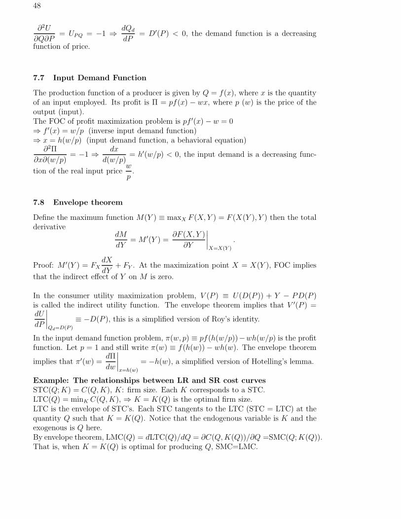
48
∂2U
∂Q∂P= UPQ = −1 ⇒ dQd
dP= D′(P ) < 0, the demand function is a decreasing
function of price.
7.7 Input Demand Function
The production function of a producer is given by Q = f(x), where x is the quantityof an input employed. Its profit is Π = pf(x) − wx, where p (w) is the price of theoutput (input).The FOC of profit maximization problem is pf ′(x)− w = 0⇒ f ′(x) = w/p (inverse input demand function)⇒ x = h(w/p) (input demand function, a behavioral equation)
∂2Π
∂x∂(w/p)= −1 ⇒ dx
d(w/p)= h′(w/p) < 0, the input demand is a decreasing func-
tion of the real input pricew
p.
7.8 Envelope theorem
Define the maximum function M(Y ) ≡ maxX F (X, Y ) = F (X(Y ), Y ) then the totalderivative
dM
dY= M ′(Y ) =
∂F (X, Y )
∂Y
∣
∣
∣
∣
X=X(Y )
.
Proof: M ′(Y ) = FXdX
dY+ FY . At the maximization point X = X(Y ), FOC implies
that the indirect effect of Y on M is zero.
In the consumer utility maximization problem, V (P ) ≡ U(D(P )) + Y − PD(P )is called the indirect utility function. The envelope theorem implies that V ′(P ) =dU
dP
∣
∣
∣
∣
Qd=D(P )
≡ −D(P ), this is a simplified version of Roy’s identity.
In the input demand function problem, π(w, p) ≡ pf(h(w/p))−wh(w/p) is the profitfunction. Let p = 1 and still write π(w) ≡ f(h(w))− wh(w). The envelope theorem
implies that π′(w) =dΠ
dw
∣
∣
∣
∣
x=h(w)
= −h(w), a simplified version of Hotelling’s lemma.
Example: The relationships between LR and SR cost curvesSTC(Q; K) = C(Q, K), K: firm size. Each K corresponds to a STC.LTC(Q) = minK C(Q, K), ⇒ K = K(Q) is the optimal firm size.LTC is the envelope of STC’s. Each STC tangents to the LTC (STC = LTC) at thequantity Q such that K = K(Q). Notice that the endogenous variable is K and theexogenous is Q here.By envelope theorem, LMC(Q) = dLTC(Q)/dQ = ∂C(Q, K(Q))/∂Q =SMC(Q; K(Q)).That is, when K = K(Q) is optimal for producing Q, SMC=LMC.

49
Since LAC(Q) =LTC(Q)/Q and SAC(Q) =STC(Q)/Q, LAC is the envelope of SAC’sand each SAC tangents to the LAC (SAC = LAC) at the quantity Q such thatK = K(Q).
7.9 Effect of a Unit Tax on Monopoly Output (Samuelson)
Assumptions: a monopoly firm, q = D(P ) ⇐⇒ P = f(q), (inverse functions),C = C(q), t = unit tax
max π(q) = Pq − C(q)− tq = qf(q)− C(q)− tq
q: endogenous; t: exogenousFOC: ∂π/∂q = f(q) + qf ′(q)− C ′(q)− t = 0.The FOC defines a relationship between the monopoly output q∗ and the tax rate tas q∗ = q(t) (a behavioral equation). The derivative dq∗/dt can be determined by thesign of the cross derivative:
∂2π
∂q∂t= −1 < 0
Therefore, we have dq∗/dt < 0.The result can be obtained using the q–pdiagram. FOC ⇐⇒ MR = MC + t.Therefore, on q–p space, an equilibrium is determined by the intersection point ofMR and MC + t curves.
Case 1: MR is downward sloping and MC is upward sloping:When t increases, q∗ decreases as seen from the left diagram below.
- q
6P
MC
MC+t
MR< - q
6P
MC
MC+t
MR<
Case 2: Both MR and MC are downward sloping and MR is steeper. MC decreasing;MR decreasing more ⇒ t ↑ q ↓.
Case 3: Both MR and MC are downward sloping, but MC is steeper. The diagramshows that dq∗/dt > 0. It is opposite to our comparative statics result. Why?MR = MC + t violates SOC < 0, therefore, the intersection of MR and MC + tis not a profit maximizing point.
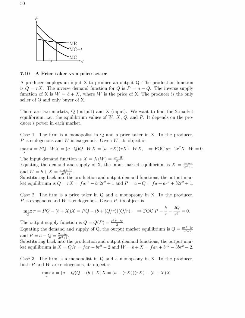
50
- q
6P
MC
MC+tMR
>
7.10 A Price taker vs a price setter
A producer employs an input X to produce an output Q. The production functionis Q = rX. The inverse demand function for Q is P = a − Q. The inverse supplyfunction of X is W = b + X, where W is the price of X. The producer is the onlyseller of Q and only buyer of X.
There are two markets, Q (output) and X (input). We want to find the 2-marketequilibrium, i.e., the equilibrium values of W , X, Q, and P . It depends on the pro-ducer’s power in each market.
Case 1: The firm is a monopolist in Q and a price taker in X. To the producer,P is endogenous and W is exogenous. Given W , its object is
maxx
π = PQ−WX = (a−Q)Q−WX = (a−rX)(rX)−WX, ⇒ FOC ar−2r2X−W = 0.
The input demand function is X = X(W ) = ar−W2r2 .
Equating the demand and supply of X, the input market equilibrium is X = ar−b2r2+1
and W = b + X = ar+2r2b2r2+1
.Substituting back into the production and output demand functions, the output mar-ket equilibrium is Q = rX = far2 − br2r2 + 1 and P = a−Q = fa + ar2 + b2r2 + 1.
Case 2: The firm is a price taker in Q and a monopsony in X. To the producer,P is exogenous and W is endogenous. Given P , its object is
maxQ
π = PQ− (b + X)X = PQ− (b + (Q/r))(Q/r), ⇒ FOC P − b
r− 2Q
r2= 0.
The output supply function is Q = Q(P ) = r2P−br2
.
Equating the demand and supply of Q, the output market equilibrium is Q = ar2−brr2−2
and P = a−Q = 2a+br2r2+1
.Substituting back into the production and output demand functions, the output mar-ket equilibrium is X = Q/r = far − br2 − 2 and W = b + X = far + br2 − 3br2 − 2.
Case 3: The firm is a monopolist in Q and a monopsony in X. To the producer,both P and W are endogenous, its object is
maxx
π = (a−Q)Q− (b + X)X = (a− (rX))(rX)− (b + X)X.
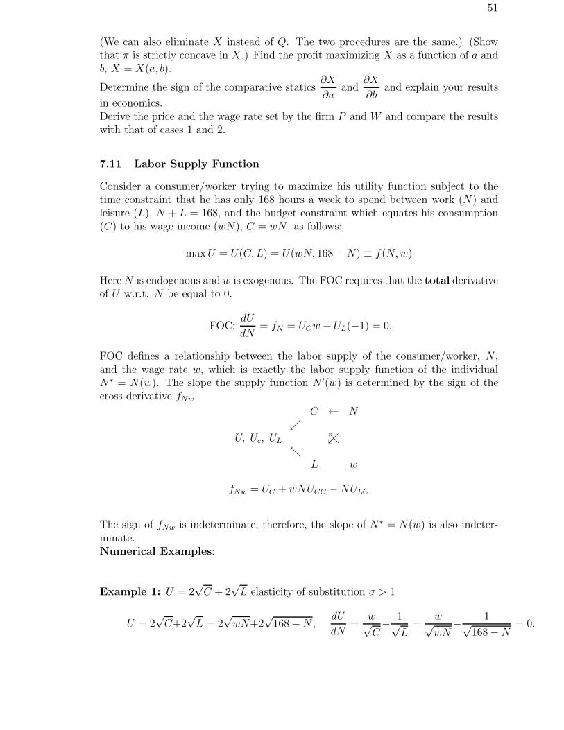
51
(We can also eliminate X instead of Q. The two procedures are the same.) (Showthat π is strictly concave in X.) Find the profit maximizing X as a function of a andb, X = X(a, b).
Determine the sign of the comparative statics∂X
∂aand
∂X
∂band explain your results
in economics.Derive the price and the wage rate set by the firm P and W and compare the resultswith that of cases 1 and 2.
7.11 Labor Supply Function
Consider a consumer/worker trying to maximize his utility function subject to thetime constraint that he has only 168 hours a week to spend between work (N) andleisure (L), N + L = 168, and the budget constraint which equates his consumption(C) to his wage income (wN), C = wN , as follows:
max U = U(C, L) = U(wN, 168−N) ≡ f(N, w)
Here N is endogenous and w is exogenous. The FOC requires that the total derivativeof U w.r.t. N be equal to 0.
FOC:dU
dN= fN = UCw + UL(−1) = 0.
FOC defines a relationship between the labor supply of the consumer/worker, N ,and the wage rate w, which is exactly the labor supply function of the individualN∗ = N(w). The slope the supply function N ′(w) is determined by the sign of thecross-derivative fNw
U, Uc, UL
C ← Nւ
ւտտ
L w
fNw = UC + wNUCC −NULC
The sign of fNw is indeterminate, therefore, the slope of N∗ = N(w) is also indeter-minate.Numerical Examples:
Example 1: U = 2√
C + 2√
L elasticity of substitution σ > 1
U = 2√
C+2√
L = 2√
wN+2√
168−N,dU
dN=
w√C− 1√
L=
w√wN− 1√
168−N= 0.

52
Therefore, the inverse labor supply function is w = N/(168 − N), which ispositively sloped.
- N
6w
σ > 1
- N
6w
σ < 1
Example 2: U = CLC+L
elasticity of substitution σ < 1
U =CL
C + L=
wN(168−N)
wN + 168−N,
dU
dN=
wL2 − C2
(C + L)2= 0.
Therefore, the inverse labor supply function is w = [(168 − N)/N ]2, which isnegatively sloped.
Example 3: U = CL Cobb-Douglas( σ = 1)
U = CL = wN(168−N)dU
dN= w(168− 2N) = 0
The labor supply function is a constant N = 84 and the curve is vertical.
- N
6w
σ = 1
- N
6w
Backward-bending Labor Supply Curve: It is believed that the labor supplycurve can be backward-bending.
7.12 Exponential and logarithmic functions and interest compounding
Exponential function f(x) = ex is characterized by f(0) = 1 and f(x) = f ′(x) =f ′′(x) = . . . = f (n)(x). The Taylor expansion of the exponential functionat x = 0becomes
ex = 1 + x + x2/2! + · · ·+ xn/n! + . . .
Some Rules:d
dx(ex) = ex,
d
dxeax = aeax,
d
dxef(x) = f ′(x)ef(x).

53
The inverse of ex is the logarithmic function: ln x. If x = ey, then we define y ≡ lnx.
More generally, if x = ay, a > 0, then we define y ≡ loga x =ln x
ln a.
Using inverse function rule: dx = eydy,d
dxln x =
1
eln x= 1/x.
- x
6y
��
��
��
��
��
��
��
��
��
��
y = ex
y = ln x
ax = eln ax
= e(ln a)x ⇒ d
dxax = (ln a)e(ln a)x = (ln a)ax.
d
dxlna x =
(
1
ln a
)
1
x
growth rate of a function of time y = f(t):
growth rate ≡ 1
y
dy
dt=
f ′
f=
d
dt[ln f(t)].
Example: f(t) = g(t)h(t). ln f(t) = ln g(t) + ln h(t), therefore, growth rate of f(t) isequal to the sum of the growth rates of g(t) and h(t).
Interest compoundingA: principal (PV), V = Future Value, r = interest rate, n = number of periods
V = A(1 + r)n
If we compound interest m times per period, then the interest rate each time becomesr/m, the number of times of compounding becomes mn, and
V = A[(1 + r/m)m]n
limm→∞
(1 + r/m)m = 1 + r + r2/2! + · · ·+ rn/n! + . . . = er
Therefore, V → Aern, this is the formula for instantaneous compounding.

54
7.13 Timing: (when to cut a tree)
t: number of years to wait, A(t) present value after t years
V (t) = Ke√
t: the market value of the tree after t years
A(t) = Ke√
te−rt is the present valueWe want to find the optimal t such that the present value is maximized.
maxt
A(t) = Ke√
te−rt.
The FOC is
A′ =
(
1
2√
t− r
)
A(t) = 0
Because A(t) 6= 0, FOC implies:1
2√
t− r = 0, t∗ = 1/(4r2)
For example, if r = 10%, t = 25, then to wait 25 years before cutting the tree is theoptimum.Suppose that A(t) = ef(t)
FOC becomes: A′(t)/A(t) = f ′(t) = r, ⇒ f ′(t) is the instantaneous growth rate (orthe marginal growth rate) at t, ⇒ at t = 25, growth rate = 10% = r, at t = 26,growth rate < 10%. Therefore, it is better to cut and sell the tree at t = 25 and putthe proceed in the bank than waiting longer.SOC: It can be shown that A′′ < 0.
7.14 Problems
1. Suppose the total cost function of a competitive firm is C(Q) = eaQ+b. Derivethe supply function.
2. The input demand function of a competitive producer, X = X(W ), can bederived by maximizing the profit function Π = F (X) −WX with respect toX, where X is the quantity of input X and W is the price of X. Derive thecomparative statics dX/dW and determine its sign.
3. The utility function of a consumer is given by U = U(X) + M , where X is thequantity of commodity X consumed and M is money. Suppose that the totalincome of the consumer is $ 100 and that the price of X is P . Then the utilityfunction become U(X) + (100−XP ).
(a) Find the first order condition of the utility maximization problem.
(b) What is the behavior equation implied by the first order condition?
(c) Derive dX/dP and determine its sign. What is the economic meaning ofyour result?
4. The consumption function of a consumer, C = C(Y ), can be derived by max-imizing the utility function U(C, Y ) = u1(C) + u2(Y − C), where u′
1(C) > 0,u′
2(Y −C) > 0 and u1”(C) < 0, u2”(Y −C) < 0. Derive the comparative staticsdC/dY and determine its sign.

55
5. Consider a duopoly market with two firms, A and B. The inverse demand func-tion is P = f(QA + QB), f ′ < 0, f” < 0. The cost function of firm A is TCA
= C(QA), C ′ > 0, C” > 0. The profit of firm A is ΠA = PQA − TCA =QAf(QA +QB)−C(QA). For a given output of firm B, QB, there is a QA whichmaximizes firm A’s profit. This relationship between QB and QA is called thereaction function of firm A, QA = RA(QB).
(a) Find the slope of the reaction function R′A = dQA
dQB.
(b) When QB increases, will firm A’s output QA increase or decrease?
6. The profit of a monopolistic firm is given by Π = R(x) − C(x, b), where x isoutput, b is the price of oil, R(x) is total revenue, and C(x, b) is the total costfunction. For any given oil price b, there is an optimal
output which maximizes profit, that is, the optimal output is a function of oilprice, x = x(b). Assume that Cbx = ∂2C/∂b∂x > 0, that is, an increase in oilprice will increase marginal cost. Will an increase in oil price increase output,that is, is dx/db > 0?
7. Consider a monopsony who uses a single input, labor (L), for the production of acommodity (Q), which he sells in a perfect competition market. His productionfunction is Q = F (L), (f ′(L) > 0). The labor supply function is L = L(w), ormore convenient for this problem, w = L−1(L) = W (L). Given the commodityprice p, there is an optimal labor input which maximizes the monopsonist’stotal profit Π = pf(L)−W (L)L. In this problem, you are asked to derive therelation between L and p.
(a) State the FOC and the SOC of the profit maximization problem.
(b) Derive the comparative statics dL/dp and determine its sign.
8. Suppose that a union has a fixed supply of labor (L) to sell, that unemployedworkers are paid unemployment insurance at a rate of $u per worker, and thatthe union wishes to maximize the sum of the wage bill plus the unemploymentcompensation S = wD(w) + u(L−D(w)), where w is wage per
worker, D(w) is labor demand function, and D′(w) < 0. Show that if u in-creases, then the union should set a higher w. (Hint: w is endogenous and u isexogenous.)
9. The production function of a competitive firm is given by Q = F (L, K). whereL is variable input and K is fixed input. The short run profit function is givenby Π = pQ−wL−rK, where p is output price, w is wage rate, and r is the rentalrate on capital. In the short run, given the quantity of fixed input K,there is aL which maximizes Π. Hence, the short run demand for L can be regarded asa function of K. Assume that FLK > 0.
(a) State the FOC and SOC of the profit maximization problem.
(b) Derive the comparative statics dL/dK and determine its sign.
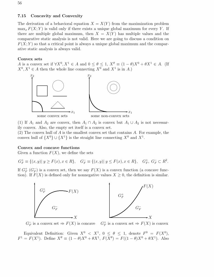
56
7.15 Concavity and Convexity
The derivation of a behavioral equation X = X(Y ) from the maximization problemmaxx F (X; Y ) is valid only if there exists a unique global maximum for every Y . Ifthere are multiple global maximum, then X = X(Y ) has multiple values and thecomparative static analysis is not valid. Here we are going to discuss a condition onF (X; Y ) so that a critical point is always a unique global maximum and the compar-ative static analysis is always valid.
Convex setsA is a convex set if ∀X0, X1 ∈ A and 0 ≤ θ ≤ 1, Xθ ≡ (1 − θ)X0 + θX1 ∈ A. (IfX0, X1 ∈ A then the whole line connecting X0 and X1 is in A.)
-x1
6x2
@@�
�
some convex sets
����
- x1
6x2
����"!#
some non-convex sets
(1) If A1 and A2 are convex, then A1 ∩ A2 is convex but A1 ∪ A2 is not necessar-ily convex. Also, the empty set itself is a convex set.(2) The convex hull of A is the smallest convex set that contains A. For example, theconvex hull of {X0} ∪ {X1} is the straight line connecting X0 and X1.
Convex and concave functionsGiven a function F (X), we define the sets
G+F ≡ {(x, y)| y ≥ F (x), x ∈ R}, G−
F ≡ {(x, y)| y ≤ F (x), x ∈ R}, G+F , G−
F ⊂ R2.
If G+F (G−
F ) is a convex set, then we say F (X) is a convex function (a concave func-tion). If F (X) is defined only for nonnegative values X ≥ 0, the definition is similar.
-X
6
F (X)
G−F
G+F
G−F is a convex set ⇒ F (X) is concave
- X
6 F (X)
G−F
G+F
G+F is a convex set ⇒ F (X) is convex
Equivalent Definition: Given X0 < X1, 0 ≤ θ ≤ 1, denote F 0 = F (X0),F 1 = F (X1). Define Xθ ≡ (1 − θ)X0 + θX1, F (Xθ) = F ((1 − θ)X0 + θX1). Also

57
define F θ ≡ (1− θ)F (X0) + θF (X1) = (1− θ)F 0 + θF 1.
-X
6 F (X)
X0 Xθ X1
F 0 = F (X0)
F (Xθ)
F 1 = F (X1)
- X
6
��
��
��
��
�
X0 Xθ X1
F 0
F θ
F 1
Xθ −X0
X1 −Xθ=
θ(X1 −X0)
(1− θ)(X1 −X0)=
θ
1− θ,
F θ − F 0
F 1 − F θ=
θ(F 1 − F 0)
(1− θ)(F 1 − F 0)=
θ
1− θ.
Therefore, (Xθ, F θ) is located on the straight line connecting (X0, F 0) and (X1, F 1)and when θ shifts from 0 to 1, (Xθ, F θ) shifts from (X0, F 0) to (X1, F 1) (the rightfigure). On the other hand, (Xθ, F (Xθ)) shifts along the curve representing the graphof F (X) (the left figure). Put the two figures together:
-X
6 F (X)
X0 Xθ X1
��
��
��
��
�
F θ
F (Xθ)
F (X) is strictly concave ⇒ if for all X0, X1 and θ ∈ (0, 1), F (Xθ) > F θ.F (X) is concave ⇒ if for all X0, X1 and θ ∈ [0, 1], F (Xθ) ≥ F θ.
-X
6
F (X)
F (X) is strictly
concave- X
6
F (X)F (X) is concave(not strictly)
Notice that these concepts are global concepts. (They have something to do with thewhole graph of F , not just the behavior of F nearby a point.) The graph of a concavefunction can have a flat part. For a strictly concave function, the graph should becurved everywhere except at kink points.
F (X) is strictly convex ⇒ if for all X0, X1 and θ ∈ (0, 1), F (Xθ) < F θ.F (X) is convex ⇒ if for all X0, X1 and θ ∈ [0, 1], F (Xθ) ≤ F θ.

58
-X
6F
F (X) is strictly
convex
- X
6F
H
F (X) is convex
(not strictly)
Remark 1: A linear function is both concave and convex since F θ ≡ F (Xθ).
-X
6F
���������
- X
6F
��������
�����
a concavepiecewise-linearfunction
- X
6F
�����
��������
a convexpiecewise-linearfunction
Remark 2: A piecewise-linear function consists of linear components; for example,the income tax schedule T = f(Y ) is a piecewise-linear function. Other examples are
concave F (X) =
{
2X X ≤ 11 + X X > 1
convex F (X) =
{
X X ≤ 12X − 1 X > 1
In the following theorems, we assume that F ′′(X) exists for all X.
Theorem 1: F (X) is concave, ⇔ F ′′(X) ≤ 0 for all X.F ′′(X) < 0 for all X ⇒ F (X) is strictly concave.Proof: By Taylor’s theorem, there exist X0 ∈ [X0, Xθ] and X1 ∈ [Xθ, X1] such that
F (X1) = F (Xθ) + F ′(Xθ)(X1 −Xθ) +1
2F ′′(X1)(X1 −Xθ)2
F (X0) = F (Xθ) + F ′(Xθ)(X0 −Xθ) +1
2F ′′(X0)(X0 −Xθ)2
⇒ F θ = F (Xθ) +1
2θ(1− θ)(X1 −X0)2[F ′′(X0) + F ′′(X1)].
Theorem 2: If F (X) is concave and F ′(X0) = 0, then X0 is a global maximum.If F (X) is strictly concave and F ′(X0) = 0, then X0 is a unique global maximum.Proof: By theorem 1, X0 must be a local maximum. If it is not a global maximum,then there exists X1 such that F (X1) > F (X0), which implies that F (Xθ) > F (X0)for θ close to 0. Therefore, X0 is not a local maximum, a contradiction.
Remark 1 (boundary/corner solution): The boundary or corner condition F ′(X) ≤ 0,

59
XF ′(X) = 0 (or F ′(X) ≥ 0, (X − a)F ′(X) = 0) becomes sufficient for global maxi-mum.
Remark 2 (minimization problem): For the minimization problem, we replace con-cavity with convexity and F ′′(X) < 0 with F ′′(X) > 0. If F (X) is convex andF ′(X∗) = 0, then X∗ is a global minimum.If F (X) is strictly convex and F ′(X∗) = 0, then X∗ is a unique global minimum.
Remark 3: The sum of two concave functions is concave. The product of two concavefunction is not necesarily concave. Xa is strictly concave if a < 1, strictly convex ifa > 1. eX is strictly convex and ln X is strctly concave with X > 0.
-X
6F
Xa, a > 1
- X
6F
Xa, 0 < a < 1
- X
6F
Xa, a < 0
-X
6F
eaX
- X
6F
ln X- X
6F
−aX2 + bX + c
Remark 4: A concave function does not have to be differentiable, but it must becontinuous on the interior points.
7.16 Indeterminate forms and L’Hopital’s rule
Let f(x) =g(x)
h(x), g(a) = h(a) = 0 and g(x) and h(x) be continuous at x = a. f(a) is
not defined because it is0
0. However, limx→a f(x) can be calculated.
limx→a
f(x) = limx→a
g(x)
h(x)= lim
x→a
g(x)− g(a)
h(x)− h(a)= lim
∆x→0
g(a + ∆x)− g(a)
h(a + ∆x)− h(a)=
g′(a)
h′(a).
The same procedure also works for the case with g(a) = h(a) =∞.
Example 1: f(x) =g(x)
h(x)=
ln[(ax + 1)/2]
x,
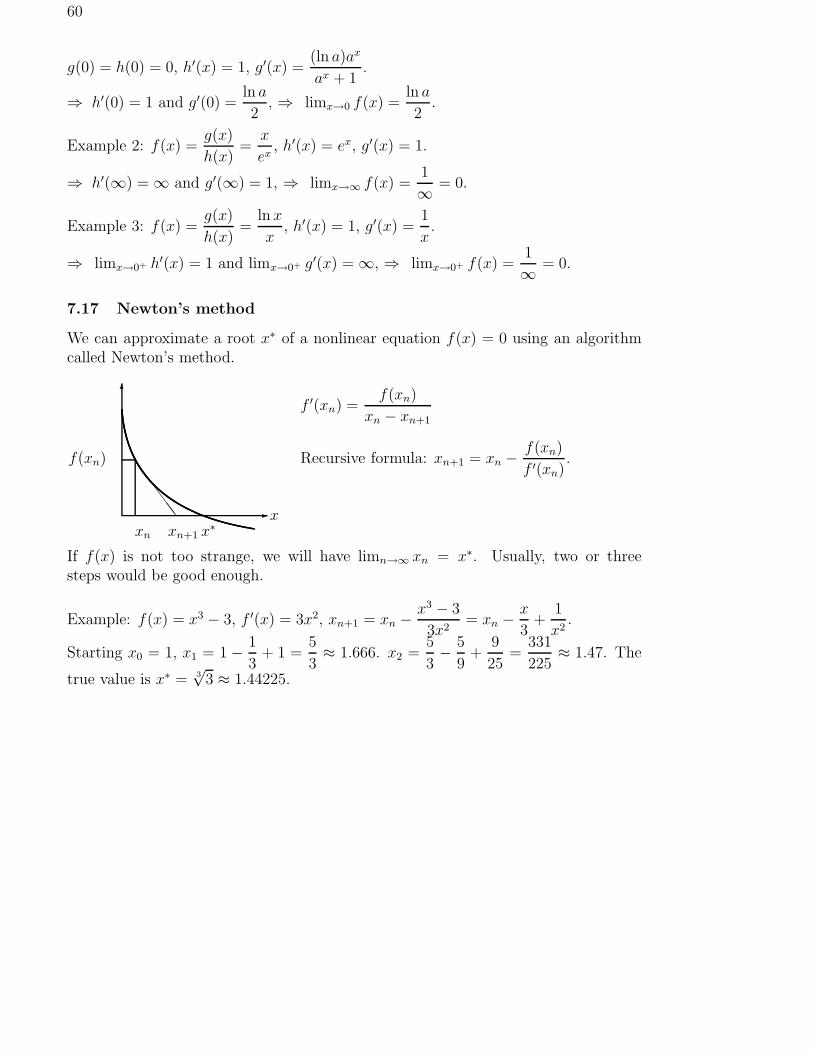
60
g(0) = h(0) = 0, h′(x) = 1, g′(x) =(ln a)ax
ax + 1.
⇒ h′(0) = 1 and g′(0) =ln a
2, ⇒ limx→0 f(x) =
ln a
2.
Example 2: f(x) =g(x)
h(x)=
x
ex, h′(x) = ex, g′(x) = 1.
⇒ h′(∞) =∞ and g′(∞) = 1, ⇒ limx→∞ f(x) =1
∞ = 0.
Example 3: f(x) =g(x)
h(x)=
ln x
x, h′(x) = 1, g′(x) =
1
x.
⇒ limx→0+ h′(x) = 1 and limx→0+ g′(x) =∞, ⇒ limx→0+ f(x) =1
∞ = 0.
7.17 Newton’s method
We can approximate a root x∗ of a nonlinear equation f(x) = 0 using an algorithmcalled Newton’s method.
-x
6
xn xn+1 x∗
f(xn)S
SS
SS
f ′(xn) =f(xn)
xn − xn+1
Recursive formula: xn+1 = xn −f(xn)
f ′(xn).
If f(x) is not too strange, we will have limn→∞ xn = x∗. Usually, two or threesteps would be good enough.
Example: f(x) = x3 − 3, f ′(x) = 3x2, xn+1 = xn −x3 − 3
3x2= xn −
x
3+
1
x2.
Starting x0 = 1, x1 = 1− 1
3+ 1 =
5
3≈ 1.666. x2 =
5
3− 5
9+
9
25=
331
225≈ 1.47. The
true value is x∗ = 3√
3 ≈ 1.44225.

61
8 Optimization–Multivariate Case
Suppose that the objective function has n variables: maxx1,...,xn
F (x1, . . . , xn) = F (X).
A local maximum X∗ = (x∗1, . . . , x
∗n): ∃ǫ > 0 such that F (X∗) ≥ F (X) for all X
satisfying xi ∈ (x∗i − ǫ, x∗
i + ǫ) ∀i.A critical point Xc = (xc
1, . . . , xcn):
∂F (Xc)
∂xi
= 0 ∀i.A global maximum X∗: F (X∗) ≥ F (X) ∀X.A unique global maximum X∗: F (X∗) > F (X) ∀X 6= X∗.The procedure is the same as that of the single variable case. (1) Use FOC to findcritical points; (2) use SOC to check whether a critical point is a local maximum, orshow that F (X) is concave so that a critical point must be a global maximum.
If we regard variables other than xi as fixed, then it is a single variable maximizationproblem and, therefore, we have the necessary conditions
FOC:∂F
∂xi= 0 and SOC:
∂2F
∂x2i
< 0, i = 1, . . . , n.
However, since there are n×n second order derivatives (the Hessian matrix H(F )) andthe SOC above does not consider the cross-derivatives, we have a reason to suspectthat the SOC is not sufficient. In the next section we will provide a counter-exampleand give a true SOC.
8.1 SOC
SOC of variable-wise maximization is wrongExample: max
x1,x2
F (x1, x2) = −x21 + 4x1x2 − x2
2.
FOC: F1 = −2x1 + 4x2 = 0, F2 = 4x1 − 2x2 = 0, ⇒ x1 = x2 = 0.SOC? F11 = F22 = −2 < 0.
- x1
6x2
��������������������
��������������������
4
1
4
1
-4-1
-4-1
(0,0) isa saddle point.
- xi
6F
When xj = 0,xi = 0 is
a maximum.

62
F (0, 0) = 0 < F (k, k) = 2k2 for all k 6= 0. ⇒ (0, 0) is not a local maximum!The true SOC should take into consideration the possibility that when x1 and x2
increase simultaneously F may increase even if individual changes cannot increase F .
SOC of sequential maximization:We can solve the maximization problem sequentially. That is, for a given x2, wecan find a x1 such that F (x1, x2) is maximized. The FOC and SOC are F1 = 0 andF11 < 0. The solution depends on x2, x1 = h(x2), i.e., we regard x1 as endogenousvariable and x2 as an exogenous variable in the first stage. Using implicit functionrule, dx1/dx2 = h′(x2) = −F12/F11. In the second stage we maximize M(x2) ≡F (h(x2), x2). The FOC is M ′(x2) = F1h
′ + F2 = F2 = 0 (since F1 = 0). The SOC is
M ′′(x2) = F1h′′ + F11(h
′)2 + 2F12h′ + F22 = (−F 2
12 + F11F22)/F11 < 0.
Therefore, the true SOC is: F11 < 0 and F11F22 − F 212 > 0.
For the n-variable case, the sequential argument is more complicated and we use Tay-lor’s expansion.
SOC using Taylor’s expansion:To find the true SOC, we can also use Taylor’s theorem to expand F (X) around acritical point X∗:
F (X) = F (X∗) + F1(X∗)(x1 − x∗
1) + F2(X∗)(x2 − x∗
2)
+1
2(x1 − x∗
1, x2 − x∗2)
(
F11(X∗) F12(X
∗)F21(X
∗) F22(X∗)
)(
x1 − x∗1
x2 − x∗2
)
+ higher order terms.
Since X∗ is a critical point, F1(X∗) = F2(X
∗) = 0 and we have the approximationfor X close to X∗:
F (X)− F (X∗) ≈ 1
2(x1 − x∗
1, x2 − x∗2)
(
F11(X∗) F12(X
∗)F21(X
∗) F22(X∗)
)(
x1 − x∗1
x2 − x∗2
)
≡ 1
2v′H∗v.
True SOC: v′H∗v < 0 for all v 6= 0.
In the next section, we will derive a systematic method to test the true SOC.
8.2 Quadratic forms and their signs
A quadratic form in n variables is a second degree homogenous function.
f(v1, . . . , vn) =n∑
i=1
n∑
j=1
aijvivj = (v1, . . . , vn)
a11 · · · a1n...
. . ....
an1 · · · ann
v1...vn
≡ v′Av.
Since vivj = vjvi, we can assume that aij = aji so that A is symmetrical.
Example 1: (v1 − v2)2 = v2
1 − 2v1v2 + v22 = (v1, v2)
(
1 −1−1 1
)(
v1
v2
)
.

63
Example 2: 2v1v2 = (v1, v2)
(
0 11 0
)(
v1
v2
)
.
Example 3: x21 + 2x2
2 + 6x1x3 = (x1, x2, x3)
1 0 30 2 03 0 0
x1
x2
x3
.
v′Av is called negative semidefinite if v′Av ≤ 0 for all v ∈ Rn.v′Av is called negative definite if v′Av < 0 for all v 6= 0.v′Av is called positive semidefinite if v′Av ≥ 0 for all v ∈ Rn.v′Av is called positive definite if v′Av > 0 for all v 6= 0.
(1) −v21 − 2v2
2 < 0, if v1 6= 0 or v2 6= 0⇒ negative.(2) −(v1 − v2)
2 ≤ 0, = 0 if v1 = v2 ⇒ negative semidefinite.(3) (v1 + v2)
2 ≥ 0, = 0 if v1 = −v2 ⇒ positive semidefinite.(4) v2
1 + v22 > 0, if v1 6= 0 or v2 6= 0⇒ positive.
(5) v21 − v2
2
><
0 if |v1|><|v2| ⇒ neither positive nor negative definite.
(6) v1v2><
0 if sign(v1)=6= sign(v2) ⇒ neither positive nor negative definite.
Notice that if v′Av is negative (positive) definite then it must be negative (positive)semidefinite.Testing the sign of a quadratic form:
n = 2: v′Av = (v1, v2)
(
a11 a12
a21 a22
)(
v1
v2
)
= a11v21 + 2a12v1v2 + a22v
22 =
a11
(
v21 + 2
a12
a11v1v2 +
a212
a211
v22
)
+
(
−a212
a11+ a22
)
v22 = a11
(
v1 +a12
a11v2
)2
+
∣
∣
∣
∣
a11 a12
a21 a22
∣
∣
∣
∣
a11v22 .
Negative definite ⇔ a11 < 0 and
∣
∣
∣
∣
a11 a12
a21 a22
∣
∣
∣
∣
= a11a22 − a212 > 0.
Positive definite ⇔ a11 > 0 and
∣
∣
∣
∣
a11 a12
a21 a22
∣
∣
∣
∣
= a11a22 − a212 > 0.
For negative or positive semidefinite, replace strict inequalities with semi-inequalities.The proofs for them are more difficult and discussed in Lecture 13.
Example 1: F (v1, v2) = −2v21 + 8v1v2 − 2v2
2 = (v1, v2)
(
−2 44 −2
)(
v1
v2
)
, a11 =
−2 < 0 but
∣
∣
∣
∣
−2 44 −2
∣
∣
∣
∣
= −12 < 0 ⇒ neither positive nor negative. The matrix is
the Hessian of F of the counter-example in section 1. Therefore, the counter-exampleviolates the SOC.

64
General n: v′Av = (v1, . . . , vn)
a11 · · · a1n...
. . ....
an1 · · · ann
v1...
vn
= a11(v1 + · · ·)2
+
∣
∣
∣
∣
a11 a12
a21 a22
∣
∣
∣
∣
a11(v2+· · ·)2+
∣
∣
∣
∣
∣
∣
a11 a12 a13
a21 a22 a23
a31 a32 a33
∣
∣
∣
∣
∣
∣
∣
∣
∣
∣
a11 a12
a21 a22
∣
∣
∣
∣
(v3+· · ·)2+· · ·+
∣
∣
∣
∣
∣
∣
∣
a11 · · · a1n...
. . . · · ·an1 · · · ann
∣
∣
∣
∣
∣
∣
∣
∣
∣
∣
∣
∣
∣
∣
a11 · · · a1(n−1)...
. . ....
a(n−1)1 · · · a(n−1)(n−1)
∣
∣
∣
∣
∣
∣
∣
v2n.
k-th order principle minor of A: A(k) ≡
a11 · · · a1k...
. . ....
ak1 · · · akk
, k = 1, . . . , n.
Negative definite ⇔ A(1) = a11 < 0,|A(2)||A(1)| < 0,
|A(3)||A(2)| < 0, . . .,
|A(n)||A(n−1)| < 0.
Positive definite ⇔ A(1) = a11 > 0,|A(2)||A(1)| > 0,
|A(3)||A(2)| > 0, . . .,
|A(n)||A(n−1)| > 0.
Negative definite ⇔ |A(1)| = a11 < 0, |A(2)| =
∣
∣
∣
∣
a11 a12
a21 a22
∣
∣
∣
∣
> 0, |A(3)| =
∣
∣
∣
∣
∣
∣
a11 a12 a13
a21 a22 a23
a31 a32 a33
∣
∣
∣
∣
∣
∣
< 0, · · ·, (−1)n|A(n)| = (−1)n
∣
∣
∣
∣
∣
∣
∣
a11 · · · a1n...
. . ....
an1 · · · ann
∣
∣
∣
∣
∣
∣
∣
> 0.
Positive definite ⇔ |A(1)| = a11 > 0, |A(2)| =
∣
∣
∣
∣
a11 a12
a21 a22
∣
∣
∣
∣
> 0, |A(3)| =
∣
∣
∣
∣
∣
∣
a11 a12 a13
a21 a22 a23
a31 a32 a33
∣
∣
∣
∣
∣
∣
> 0, · · ·, |A(n)| =
∣
∣
∣
∣
∣
∣
∣
a11 · · · a1n...
. . ....
an1 · · · ann
∣
∣
∣
∣
∣
∣
∣
> 0.
The conditions for semidefinite are more complicated and will be discussed in Lecture13 using the concept of eigenvalues of a square matrix.
8.3 SOC again
From the last two sections, the SOC for a local maximum can be summarized as:
SOC: v′HF (X∗)v is negative definite ⇒ F11(X∗) < 0,
∣
∣
∣
∣
F11(X∗) F12(X
∗)F21(X
∗) F22(X∗)
∣
∣
∣
∣
=
F11F22 − F 212 > 0,
∣
∣
∣
∣
∣
∣
F11(X∗) F12(X
∗) F13(X∗)
F21(X∗) F22(X
∗) F23(X∗)
F31(X∗) F32(X
∗) F33(X∗)
∣
∣
∣
∣
∣
∣
< 0, . . .
Example: maxF (x1, x2) = 3x1 + 3x1x2 − 3x21 − x3
2. (A cubic function in 2 vari-ables.)
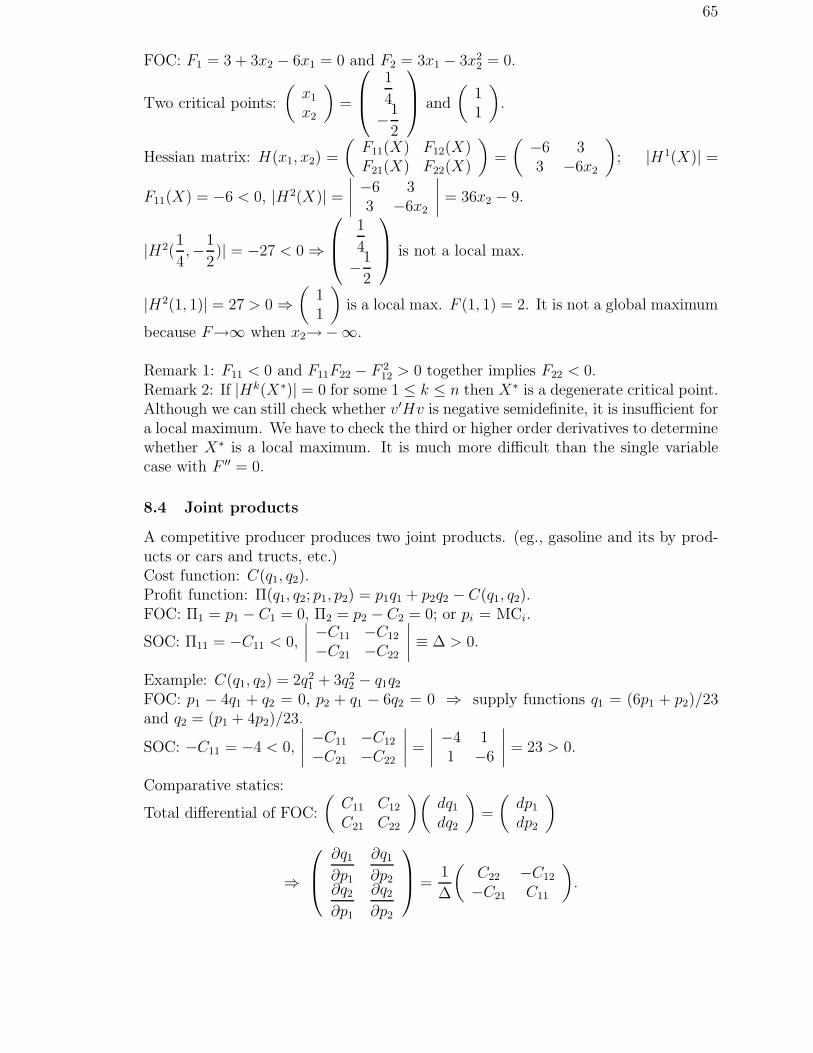
65
FOC: F1 = 3 + 3x2 − 6x1 = 0 and F2 = 3x1 − 3x22 = 0.
Two critical points:
(
x1
x2
)
=
1
4
−1
2
and
(
11
)
.
Hessian matrix: H(x1, x2) =
(
F11(X) F12(X)F21(X) F22(X)
)
=
(
−6 33 −6x2
)
; |H1(X)| =
F11(X) = −6 < 0, |H2(X)| =∣
∣
∣
∣
−6 33 −6x2
∣
∣
∣
∣
= 36x2 − 9.
|H2(1
4,−1
2)| = −27 < 0⇒
1
4
−1
2
is not a local max.
|H2(1, 1)| = 27 > 0⇒(
11
)
is a local max. F (1, 1) = 2. It is not a global maximum
because F→∞ when x2→−∞.
Remark 1: F11 < 0 and F11F22 − F 212 > 0 together implies F22 < 0.
Remark 2: If |Hk(X∗)| = 0 for some 1 ≤ k ≤ n then X∗ is a degenerate critical point.Although we can still check whether v′Hv is negative semidefinite, it is insufficient fora local maximum. We have to check the third or higher order derivatives to determinewhether X∗ is a local maximum. It is much more difficult than the single variablecase with F ′′ = 0.
8.4 Joint products
A competitive producer produces two joint products. (eg., gasoline and its by prod-ucts or cars and tructs, etc.)Cost function: C(q1, q2).Profit function: Π(q1, q2; p1, p2) = p1q1 + p2q2 − C(q1, q2).FOC: Π1 = p1 − C1 = 0, Π2 = p2 − C2 = 0; or pi = MCi.
SOC: Π11 = −C11 < 0,
∣
∣
∣
∣
−C11 −C12
−C21 −C22
∣
∣
∣
∣
≡ ∆ > 0.
Example: C(q1, q2) = 2q21 + 3q2
2 − q1q2
FOC: p1 − 4q1 + q2 = 0, p2 + q1 − 6q2 = 0 ⇒ supply functions q1 = (6p1 + p2)/23and q2 = (p1 + 4p2)/23.
SOC: −C11 = −4 < 0,
∣
∣
∣
∣
−C11 −C12
−C21 −C22
∣
∣
∣
∣
=
∣
∣
∣
∣
−4 11 −6
∣
∣
∣
∣
= 23 > 0.
Comparative statics:
Total differential of FOC:
(
C11 C12
C21 C22
)(
dq1
dq2
)
=
(
dp1
dp2
)
⇒
∂q1
∂p1
∂q1
∂p2∂q2
∂p1
∂q2
∂p2
=
1
∆
(
C22 −C12
−C21 C11
)
.
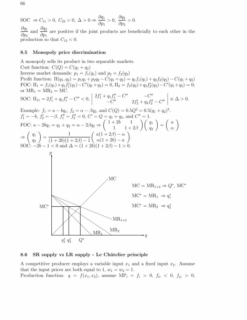
66
SOC ⇒ C11 > 0, C22 > 0, ∆ > 0⇒ ∂q1
∂p1> 0,
∂q2
∂p2> 0.
∂q1
∂p2
and∂q2
∂p1
are positive if the joint products are beneficially to each other in the
production so that C12 < 0.
8.5 Monopoly price discrimination
A monopoly sells its product in two separable markets.Cost function: C(Q) = C(q1 + q2)Inverse market demands: p1 = f1(q1) and p2 = f2(q2)Profit function: Π(q1, q2) = p1q1 + p2q2−C(q1 + q2) = q1f1(q1)+ q2f2(q2)−C(q1 + q2)FOC: Π1 = f1(q1)+q1f
′1(q1)−C ′(q1+q2) = 0, Π2 = f2(q2)+q2f
′2(q2)−C ′(q1 +q2) = 0;
or MR1 = MR2 = MC.
SOC: Π11 = 2f ′1 + q1f
′′1 − C ′′ < 0,
∣
∣
∣
∣
2f ′1 + q1f
′′1 − C ′′ −C ′′
−C ′′ 2f ′2 + q2f
′′2 − C ′′
∣
∣
∣
∣
≡ ∆ > 0.
Example: f1 = a− bq1, f2 = α− βq2, and C(Q) = 0.5Q2 = 0.5(q1 + q2)2.
f ′1 = −b, f ′
2 = −β, f ′′1 = f ′′
2 = 0, C ′ = Q = q1 + q2, and C ′′ = 1.
FOC: a− 2bq1 = q1 + q2 = α− 2βq2 ⇒(
1 + 2b 11 1 + 2β
)(
q1
q2
)
=
(
aα
)
⇒(
q1
q2
)
=1
(1 + 2b)(1 + 2β)− 1
(
a(1 + 2β)− αα(1 + 2b)− a
)
.
SOC: −2b− 1 < 0 and ∆ = (1 + 2b)(1 + 2β)− 1 > 0.
- q
6p
��
��
��
��
��
��
��
MC
@@
@@
@@
@@
@@ MR1
QMR2
aaaaaaaaaaaaaaa MR1+2
Q∗q∗2q∗1
MC∗
MC = MR1+2 ⇒ Q∗, MC∗
MC∗ = MR1 ⇒ q∗1
MC∗ = MR2 ⇒ q∗2
8.6 SR supply vs LR supply - Le Chatelier principle
A competitive producer employs a variable input x1 and a fixed input x2. Assumethat the input prices are both equal to 1, w1 = w2 = 1.Production function: q = f(x1, x2), assume MPi = fi > 0, fii < 0, fij > 0,

67
f11f22 > f 212.
Profit function: Π(x1, x2; p) = pf(x1, x2)− x1 − x2.
Short-run problem (only x1 can be adjusted, x2 is fixed):SR FOC: Π1 = pf1 − 1 = 0, or w1 = VMP1. SOC: Π11 = pf11 < 0,
Comparative statics: f1dp+pf11dx1 = 0⇒dx1
dp=−f1
pf11
> 0,dqs
dp=−f 2
1
pf11
=−1
p3f11
> 0.
Long-run problem (both x1 and x2 can be adjusted):LR FOC: Π1 = pf1 − 1 = 0, Π2 = pf2 − 1 = 0; or wi = VMPi.
SOC: Π11 = pf11 < 0,
∣
∣
∣
∣
pf11 pf12
pf21 pf22
∣
∣
∣
∣
≡ ∆ > 0.
Comparative statics:
(
f1dpf2dp
)
+
(
pf11 pf12
pf21 pf22
)(
dx1
dx2
)
=
(
00
)
⇒(
dx1/dpdx2/dp
)
=−1
p(f11f22 − f 212)
(
f1f22 − f2f12
f2f11 − f1f21
)
,dqL
dp=−(f11 + f22 − 2f12)
p3(f11f22 − f 212)
Le Chatelier principle:dqL
dp>
dqs
dp.
Example: f(x1, x2) = 3x1/31 x
1/32 (homogenous of degree 2/3)
LR FOC: px−2/31 x
1/32 = 1 = px
1/31 x
−2/32 ⇒ x1 = x2 = p3 qL = 3p2.
SR FOC (assuming x2 = 1): px−2/31 = 1⇒ x1 = p3/2 qs = 3p1/2.
ηL (LR supply elasticity) = 2 > ηs (SR supply elasticity) = 1/2.
- q
6p
Ss(p) = 3p0.5
SL(p) = 3p2
- p
6π
���������� πL(p)
πs(p; x2)
h(p)
p
Envelop theorem, Hotelling’s lemma, and Le Chatelier principleFrom the SR problem we first derive the SR variable input demand function x1 =x1(p, x2).Then the SR supply function is obtained by substituting into the production functionqs = f(x1(p, x2), x2) ≡ Ss(p; x2).The SR profit function is πs(p, x2) = pqs − x1(p, x2)− x2.
Hotelling’s lemma: By envelop theorem,∂πs
∂p= Ss(p, x2).
From the LR problem we first derive the input demand functions x1 = x1(p) andx2 = x2(p).Then the LR supply function is obtained by substituting into the production function

68
qL = f(x1(p), x2(p)) ≡ SL(p).The LR profit function is πL(p) = pqL − x1(p)− x2(p).
(Also Hotelling’s lemma) By envelop theorem,∂πL
∂p= SL(p).
Notice that πL(p) = πs(p; x2(p)).
Let x2 = x2(p), define h(p) ≡ πL(p) − πs(p, x2). h(p) ≥ 0 because in the LR,the producer can adjust x2 to achieve a higher profit level.Also, h(p) = 0 because πL(p) = πs(p; x2(p)) = πs(p; x2).
Therefore, h(p) has a minimum at p = p and the SOC is h′′(p) > 0 =∂2πL
∂p2−∂2πs
∂p2> 0,
which implies
Le Chatelier principle:dqL
dp− dqs
dp> 0.
8.7 Concavity and Convexity
Similar to the single variable case, we define the concepts of concavity and convexityfor 2-variable functions F (X) = F (x1, x2) by defining G+
F , G−F ⊂ R2 s follows.
G+F ≡ {(x1, x2, y)| y ≥ F (x1, x2), (x1, x2) ∈ R2}, G−
F ≡ {(x1, x2, y)| y ≤ F (x1, x2), (x1, x2) ∈ R2}.
If G+F (G−
F ) is a convex set, then we say F (X) is a convex function (a concave func-tion). If F (X) is defined only for nonnegative values x1, x2 ≥ 0, the definition issimilar. (The extension to n-variable functions is similar.)
Equivalently, given X0 =
(
x01
x02
)
, X1 =
(
x11
x12
)
, 0 ≤ θ ≤ 1, F 0 ≡ F (X0),
F 1 ≡ F (X1), we define
Xθ ≡ (1− θ)X0 + θX1 =
(
(1− θ)x01 + θx1
1
(1− θ)x02 + θx1
2
)
≡(
xθ1
xθ2
)
, F (Xθ) = F ((1− θ)X0 +
θX1)F θ ≡ (1− θ)F (X0) + θF (X1) = (1− θ)F 0 + θF 1.
-x1
6x2
@@
@@
@@
X0
Xθ
X1
x01 xθ
1 x11
x02
xθ2
x12
Xθ is located on the
straight line connecting X0 and X1,
when θ shifts from 0 to 1,
Xθ shifts from X0 to X1.
On 3-dimensional (x1–x2–F ) space, (Xθ, F θ) is located on the straight line connecting(X0, F 0) and (X1, F 1), when θ shifts from 0 to 1, (Xθ, F θ) shifts from (X0, F 0) to(X1, F 1). On the other hand, (Xθ, F (Xθ)) shifts along the surface representing thegraph of F (X).

69
F (X) is strictly concave ⇒ if for all X0, X1 and θ ∈ (0, 1), F (Xθ) > F θ.F (X) is concave ⇒ if for all X0, X1 and θ ∈ [0, 1], F (Xθ) ≥ F θ.F (X) is strictly convex ⇒ if for all X0, X1 and θ ∈ (0, 1), F (Xθ) < F θ.F (X) is convex ⇒ if for all X0, X1 and θ ∈ [0, 1], F (Xθ) ≤ F θ.
Example: 9x1/31 x
1/32 .
Assume that F is twice differentiable.Theorem 1: F (X) is concave, ⇔ v′HF v is negative semidefinite for all X.v′HFv is negative definite for all X ⇒ F (X) is strictly concave.Proof: By Taylor’s theorem, there exist X0 ∈ [X0, Xθ] and X1 ∈ [Xθ, X1] such that
F (X1) = F (Xθ) +∇F (Xθ)(X1 −Xθ) +1
2(X1 −Xθ)′HF (X1)(X1 −Xθ)
F (X0) = F (Xθ) +∇F (Xθ)(X0 −Xθ) +1
2(X0 −Xθ)′HF (X0)(X0 −Xθ)
⇒ F θ = F (Xθ) +θ(1− θ)
2(X1 −X0)′[HF (X0) + HF (X1)](X1 −X0).
Theorem 2: If F (X) is concave and ∇F (X0) = 0, then X0 is a global maximum.If F (X) is strictly concave and ∇F (X0) = 0, then X0 is a unique global maximum.Proof: By theorem 1, X0 must be a local maximum. If it is not a global maximum,then there exists X1 such that F (X1) > F (X0), which implies that F (Xθ) > F (X0)for θ close to 0. Therefore, X0 is not a local maximum, a contradiction.
Remark 1 (boundary or corner solution): The boundary or corner condition Fi(X) ≤0, xiFi(X) = 0 (or Fi(X) ≥ 0, (xi − ai)Fi(X) = 0) becomes sufficient for globalmaximum.Remark 2 (minimization problem): For the minimization problem, we replace con-cavity with convexity and negative definite with positive definite. If F (X) is convexand ∇F (X∗) = 0, then X∗ is a global minimum.If F (X) is strictly convex and ∇F (X∗) = 0, then X∗ is a unique global minimum.
8.8 Learning and utility maximization
Consumer B’s utility function is
U = u(x, k) + m− h(k), x, m, k ≥ 0,
where x is the quantity of commodity X consumed, k is B’s knowledge regard-ing the consumption of X, m is money, u(x, k) is the utility obtained, ∂2u
∂x2 < 0,∂2u∂x∂k
> 0 (marginal utility of X increases with k), and h(k) is the disutility of acquir-ing/maintaining k, h′ > 0, h′′ > 0. Assume that B has 100 dollar to spend and theprice of X is Px = 1 so that m = 100− x and U = u(x, k) + 100− x− h(k). Assume

70
also that k is fixed in the short run. The short run utility maximization problemis
maxx
u(x, k) + 100− x− h(k), ⇒ FOC:∂u
∂x− 1 = 0, SOC:
∂2u
∂x2< 0.
The short run comparative static dxdk
is derived from FOC as
dx
dk= − ∂2u/∂x2
∂2u/∂x∂k> 0,
that is, consumer B will consume more of X if B’s knowledge of X increases.
In the long run consumer B will change k to attain higher utility level. The long runutility maximization problem is
maxx,k
u(x, k) + 100− x− h(k), ⇒ FOC:∂u
∂x− 1 = 0,
∂u
∂k− h′(k) = 0.
The SOC is satisfied if we assume that u(x, k) is concave and h(k) is convex (h′′(k) >0), because F (x, k) ≡ u(x, k) + 100− x− h(k), x, k ≥ 0 is strictly concave then.
Consider now the specific case when
u(x, k) = 3x2/3k1/3 and h(k) = 0.5k2.
1. Calculate consumer B’s short run consumption of X, xs = x(k). (In this part,you may ignore the nonnegative constraint m = 100−x ≥ 0 and the possibilityof a corner solution.)x = 1/(8k).
2. Calculate the long run consumption of X, xL.x = 32
3. Derive the short run value function V (k) ≡ u(x(k), k) + 100− x(k)− h(k).
4. Solve the maximization problem maxk V (k).k = 4.
5. Explain how the SOC is satisfied and why the solution is the unique globalmaximum.
(demand functions) Consider now the general case when Px = p so that
U = 3x2/3k1/3 + 100− px− 0.5k2.
1. Calculate consumer B’s short run demand function of X, xs = x(p; k). (Warn-ing: There is a nonnegative constraint m = 100 − px ≥ 0 and you have toconsider both interior and corner cases.)xs(p) = 8kp−3 (100/p) if p ≤
√2k/5 (p <
√2k/5).
2. Calculate the long run demand function of X, xL(p). and the optimal level ofK, kL(p). (Both interior and corner cases should be considered too.)xL(p) = 32p−5 (100/p) if p > (8/25)1/4 (p < (8/25)1/4), kL(p) = [xL(p)]2/5.
71
8.9 Homogeneous and homothetic functions
A homogeneous function of degree k is f(x1, . . . , xn) such that
f(hx1, . . . , hxn) = hkf(x1, . . . , xn) ∀h > 0.
If f is homogeneous of degree k1 and g homogeneous of degree k2, then fg is homoge-
neous of degree k1 + k2,f
gis homogeneous of degree k1− k2, and fm is homogeneous
of degree mk1.
If Q = F (x1, x2) is homogeneous of degree 1, then Q = x1F (1,x2
x1) ≡ x1f
(
x2
x1
)
. If
m = H(x1, x2) is homogeneous of degree 0, then m = H(1,x2
x1) ≡ h
(
x2
x1
)
.
Euler theorem: If f(x1, . . . , xn) is homogeneous of degree k, then
x1f1 + . . . + xnfn = kf
If f is homogeneous of degree k, then fi is homogenous of degree k − 1.
Examples: 1. Cobb-Douglas function Q = Axα1 xβ
2 is homogeneous of degree α + β.
2. CES function Q = {axρ1 + bxρ
2}kρ is homogenous of degree k.
3. A quadratic form x′Ax is homogeneous of degree 2.4. Leontief function Q = min {ax1, bx2} is homogeneous of degree 1.
Homothetic functions: If f is homogeneous and g = H(f), H is a monotonicincreasing function, then g is called a homothetic function.
Example: Q = α ln x1 + β ln x2 = ln(
xα1 xβ
2
)
is homothetic.
The MRS of a homothetic function depends only on the ratiox2
x1
.
8.10 Problems
1. Use Newton’s method to find the root of the nonlinear equation X3+2X+2 = 0accurate to 2 digits.
2. Find (a) limX→0
1− 2−X
X, (b) lim
X→0+
1− e−aX
X, (c) lim
X→0
e2X − eX
X.
3. Given the total cost function C(Q) = eaQ+b, use L’hopital’s rule to find theAVC at Q = 0+.
4. Let z = x1x2 + x21 + 3x2
2 + x2x3 + x23.
(a) Use matrix multiplication to represent z.(b) Determine whether z is positive definite or negative definite.(c) Find the extreme value of z. Check whether it is a maximum or a minimum.

72
5. The cost function of a competitive producer is C(Q; K) =Q3
3K+ K, where K
is, say, the plant size (a fixed factor in the short run).
(a) At which output level, the SAC curve attains a minimum?
(b) Suppose that the equilibrium price is p = 100. The profit is Π = 100Q−Q3
3K− K. For a given K, find the supply quantity Q(K) such that SR
profit is maximized.
(c) Calculate the SR maximizing profit π(K).
(d) Find the LR optimal K = K∗ to maximize π(K).
(e) Calculate the LR supply quantity Q∗ = Q(K∗).
(f) Now solve the 2-variable maximization problem
maxQ,K≥0
Π(Q, K) = pQ− C(Q) = 100Q− Q3
3K−K.
and show that Π(Q, K) is concave so that the solution is the unique globalmaximum.
6. A competitive firm produces two joint products. The total cost function isC(q1, q2) = 2q2
1 + 3q22 − 4q1q2.
(a) Use the first order conditions for profit maximization to derive the supplyfunctions.(b) Check that the second order conditions are satisfied.
7. Check whether the function f(x, y) = ex+y is concave, convex, or neither.
8. (a) Check whether f(x, y) = 2 lnx+3 ln y−x−2y is concave, convex, or neither.(Assume that x > 0 and y > 0.)(b) Find the critical point of f .(c) Is the critical point a local maximum, a global maximum, or neither?
9. Suppose that a monopoly can produce any level of output at a constant marginalcost of $c per unit. Assume that the monopoly sells its goods in two differentmarkets which are separated by some distance. The demand curve in the firstmarket is given by Q1 = exp[−aP1] and the curve in the second market is givenby Q2 = exp[−bP2]. If the monopolist wants to maximize its total profits, whatlevel of output should be produced in each market and what price will prevail ineach market? Check that your answer is the unique global maximum. (Hints: 1.P1 = −(1/a) ln Q1 and P2 = −(1/b) ln Q2. 2. Π = P1Q1 + P2Q2− (Q1 + Q2)c =−(1/a)Q1 ln Q1 − (1/b)Q2 ln Q2 − (Q1 + Q2)c is strictly concave.)
10. The production function of a competitive firm is given by q = f(x1, x2) =
3x1
3
1 x1
3
2 , where x1 is a variable input and x2 is a fixed input. Assume that theprices of the output and the fixed input are p = w2 = 1. In the short run,the amount of the fixed input is given by x2 = x2. The profit function of thecompetitive firm is given by π = f(x1, x2)− w1x1 − x2.
73
(a) State the FOC for the SR profit maximization and calculate the SR input
demand function xS1 = xS
1 (w1) and the SR input demand elasticity w1
xS1
∂xS1
∂w1.
(b) Now consider the LR situation when x2 can be adjusted. State the FOCfor LR profit maximization and calculate the LR input demand funtion
xL1 = xL
1 (w1) and the LR input demand elasticity w1
xL1
∂xL1
∂w1.
(c) Verify the Le Chatelier principle:∣
∣
∣
w1
xL1
∂xL1
∂w1
∣
∣
∣>∣
∣
∣
w1
xS1
∂xS1
∂w1
∣
∣
∣.
(d) Show that the LR profit is a strictly concave function of (x1, x2) for x1, x2 >0 and therefore the solution must be the unique global maximum.
11. Let U(x, y) = xay + xy2, x, y, a > 0.
(a) For what value(s) of a U(x, y) is homogeneous?.
(b) For what value(s) of a U(x, y) is homothetic?

74
9 Optimization and Equality Constraints and Nonlinear Pro-gramming
In some maximization problems, the agents can choose only values of (x1, . . . , xn)that satisfy certain equalities. For example, a consumer has a budget constraintp1x1 + · · ·+ pnxn = m.
maxx1,...,xn
U(x) = U(x1, . . . , xn) subject to p1x1 + · · ·+ pnxn = m.
The procedure is the same as before. (1) Use FOC to find critical points; (2) useSOC to check whether a critical point is a local maximum, or show that U(X) isquasi-concave so that a critical point must be a global maximum.Define B = {(x1, . . . , xn) such that p1x1 + · · ·+ pnxn = m}.A local maximum X∗ = (x∗
1, . . . , x∗n): ∃ǫ > 0 such that U(X∗) ≥ U(X) for all X ∈ B
satisfying xi ∈ (x∗i − ǫ, x∗
i + ǫ) ∀i.A critical point: A X∗ ∈ B satisfying the FOC for a local maximum.A global maximum X∗: F (X∗) ≥ F (X) ∀X ∈ B.A unique global maximum X∗: F (X∗) > F (X) ∀X ∈ B, X 6= X∗.To define the concept of a critical point, we have to know what is the FOC first.
9.1 FOC and SOC for a constraint maximization
Consider the 2-variable utility maximization problem:
maxx1,x2
U(x1, x2) subject to p1x1 + p2x2 = m.
Using the budget constraint, x2 =m− p1x1
p2
= h(x1),dx2
dx1
= −p1
p2
= h′(x1), and it
becomes a single variable maximization problem:
maxx1
U
(
x1,m− p1x1
p2
)
, FOC:dU
dx1= U1 + U2
(
−p1
p2
)
= 0, SOC:d2U
dx21
< 0.
d2U
dx21
= U11 − 2p1
p2
U12 +
(
p1
p2
)2
U22 =−1
p22
∣
∣
∣
∣
∣
∣
0 −p1 −p2
−p1 U11 U12
−p2 U21 U22
∣
∣
∣
∣
∣
∣
.
By FOC,U1
p1=
U2
p2≡ λ (MU of $1).
FOC: U1 = p1λ, U2 = p2λ, SOC:
∣
∣
∣
∣
∣
∣
0 U1 U2
U1 U11 U12
U2 U21 U22
∣
∣
∣
∣
∣
∣
> 0.
Alternatively, we can define Lagrangian:
L ≡ U(x1, x2) + λ(m− p1x1 − p2x2)
75
FOC: L1 =∂L∂x1
= U1 − λp1 = 0, L2 =∂L∂x2
= U2 − λp2 = 0, Lλ =∂L∂λ
=
m− p1x1 − p2x2 = 0.
SOC:
∣
∣
∣
∣
∣
∣
0 −p1 −p2
−p1 L11 L12
−p2 L21 L22
∣
∣
∣
∣
∣
∣
> 0.
general 2-variable with 1-constraint case:
maxx1,x2
F (x1, x2) subject to g(x1, x2) = 0.
Using the constraint, x2 = h(x1),dx2
dx1= −g1
g2= h′(x1), and it becomes a single
variable maximization problem:
maxx1
F (x1, h(x1)) FOC:dF
dx1
= F1 + F2h′(x1) = 0, SOC:
d2F
dx21
< 0.
d2F
dx21
=d
dx1
(F1 + F2h′) = F11 + 2h′F12 + (h′)
2F22 + F2h
′′
h′′ =d
dx1
(
−g1
g2
)
=−1
g2
[
g11 + 2g12h′ + g22(h
′)2]
.
⇒ d2F
dx21
=
(
F11 −F2
g2
g11
)
+ 2
(
F12 −F2
g2
g12
)
h′ +
(
F22 −F2
g2
g22
)
(h′)2
= −
∣
∣
∣
∣
∣
∣
∣
∣
∣
∣
0 −h′ 1
−h′ F11 −F2
g2g11 F12 −
F2
g2g12
1 F21 −F2
g2
g21 F22 −F2
g2
g22
∣
∣
∣
∣
∣
∣
∣
∣
∣
∣
=−1
g22
∣
∣
∣
∣
∣
∣
∣
∣
∣
∣
0 g1 g2
g1 F11 −F2
g2g11 F12 −
F2
g2g12
g2 F21 −F2
g2
g21 F22 −F2
g2
g22
∣
∣
∣
∣
∣
∣
∣
∣
∣
∣
By FOC,F1
g1
=F2
g2
≡ λ (Lagrange multiplier).
Alternatively, we can define Lagrangian:
L ≡ F (x1, x2)− λg(x1, x2)
FOC: L1 =∂L∂x1
= F1−λg1 = 0, L2 =∂L∂x2
= F2− λg2 = 0, Lλ =∂L∂λ
= −g(x1, x2) =
0.
SOC:
∣
∣
∣
∣
∣
∣
0 g1 g2
g1 L11 L12
g2 L21 L22
∣
∣
∣
∣
∣
∣
> 0.
n-variable 1-constraint case:
maxx1,...,xn
F (x1, . . . , xn) subject to g(x1, . . . , xn) = 0.
L ≡ F (x1, . . . , xn)− λg(x1, . . . , xn)

76
FOC: Li =∂L∂xi
= Fi − λgi = 0, i = 1, . . . , n, Lλ =∂L∂λ
= −g(x1, . . . , xn) = 0.
SOC:
∣
∣
∣
∣
0 −g1
−g1 L11
∣
∣
∣
∣
< 0,
∣
∣
∣
∣
∣
∣
0 −g1 −g2
−g1 L11 L12
−g2 L21 L22
∣
∣
∣
∣
∣
∣
> 0
∣
∣
∣
∣
∣
∣
∣
∣
0 −g1 −g2 −g3
−g1 L11 L12 L13
−g2 L21 L22 L23
−g3 L31 L32 L33
∣
∣
∣
∣
∣
∣
∣
∣
< 0, etc.
9.2 Examples
Example 1: maxF (x1, x2) = −x21 − x2
2 subject to x1 + x2 = 1.L = −x2
1 − x22 + λ(1− x1 − x2).
FOC: L1 = −2x1 − λ = 0, L2 = −2x2 − λ = 0 and Lλ = 1− 2x1 − 2x2 = 0.
Critical point:
(
x1
x2
)
=
1
21
2
, λ = −1.
SOC:
∣
∣
∣
∣
∣
∣
0 1 11 −2 01 0 −2
∣
∣
∣
∣
∣
∣
= 4 > 0.
⇒(
1/21/2
)
is a local maximum.
- x1
6x2
@@
@@
@@
r- x1
6x2
@@
@@
@@
@@
@@
@@
@@
@@
@@
@@
@@
@@
@@
@@
@@
r
r
Example 2: maxF (x1, x2) = x1 + x2 subject to x21 + x2
2 = 1.L = x1 + x2 + λ(1− x2
1 − x22).
FOC: L1 = 1− 2λx1 = 0, L2 = 1− 2λx2 = 0 and Lλ = 1− x21 − x2
2 = 0.Two critical points: x1 = x2 = λ = 1/
√2 and x1 = x2 = λ = −1/
√2.
SOC:
∣
∣
∣
∣
∣
∣
0 −2x1 −2x2
−2x1 −2λ 0−2x2 0 −2λ
∣
∣
∣
∣
∣
∣
= 8λ(x21 + x2
2).
⇒ x1 = x2 = λ = 1/√
2 is a local maximum and x1 = x2 = λ = −1/√
2 is a localminimum.
77
9.3 Cost minimization and cost function
min C(x1, x2; w1, w2) = w1x1 + w2x2 subject to xa1x
1−a2 = q, 0 < a < 1.
L = w1x1 + w2x2 + λ(q − xa1x
1−a2 ).
FOC: L1 = w1−aλxa−11 x1−a
2 = 0, L2 = w2− (1−a)λxa1x
−a2 = 0, Lλ = q−xa
1x1−a2 = 0.
⇒ w1
w2
=ax2
(1− a)x1
⇒ x1 = q
[
aw2
(1− a)w1
]1−a
, x2 = q
[
(1− a)w1
aw2
]a
.
SOC:∣
∣
∣
∣
∣
∣
0 −axa−11 x1−a
2 −(1− a)xa1x
−a2
−axa−11 x1−a
2 a(1− a)λxa−21 x1−a
2 −a(1− a)λxa−11 x−a
2
−(1− a)xa1x
−a2 −a(1− a)λxa−1
1 x−a2 a(1− a)λxa
1x−a−12
∣
∣
∣
∣
∣
∣
= −a(1− a)q3λ
(x1x2)2< 0.
⇒ x1 = q
[
aw2
(1− a)w1
]1−a
, x2 = q
[
(1− a)w1
aw2
]a
is a local minimum.
The total cost is C(w1, w2, q) = q
[
(
a
1− a
)1−a
+
(
1− a
a
)a]
wa1w
1−a2 .
9.4 Utility maximization and demand function
max U(x1, x2) = a ln x1 + b ln x2 subject to p1x1 + p2x2 = m.L = a ln x1 + b ln x2 + λ(m− p1x1 − p2x2).
FOC: L1 =a
x1− λp1 = 0, L2 =
b
x2− λp2 = 0 and Lλ = m− p1x1 − p2x2 = 0.
⇒ a
b
x2
x1=
p1
p2⇒ x1 =
am
(a + b)p1, x2 =
bm
(a + b)p2
SOC:
∣
∣
∣
∣
∣
∣
∣
∣
∣
0 −p1 −p2
−p1−a
x21
0
−p2 0−b
x22
∣
∣
∣
∣
∣
∣
∣
∣
∣
=ap2
2
x21
+bp2
1
x22
> 0.
⇒ x1 =am
(a + b)p1
, x2 =bm
(a + b)p2
is a local maximum.
9.5 Quasi-concavity and quasi-convexity
As discussed in the intermediate microeconomics course, if the MRS is strictly de-creasing along an indifference curve (indifference curve is convex toward the origin),then the utility maximization has a unique solution. A utility function U(x1, x2)
is quasi-concave if MRS (=U1
U2) is decreasing along every indifference curve. In
case MRS is strictly decreasing, the utility function is strictly quasi-concave. IfU(x1, x2) is (strictly) quasi-concave, then a critical point must be a (unique) globalmaximum.
Two ways to determine whether U(x1, x2) is quasi-concave: (1) the set {(x1, x2) ∈R2 U(x1, x2) ≥ U} is convex for all U . (Every indifference curve is convex toward the

78
origin.)
(2)d
dx1
(
−U1
U2
)∣
∣
∣
∣
U(x1,x2)=U
> 0. (MRS is strictly decreasing along every indifference
curve.)
In sections 6.14 and 7.7 we used F (X) to define two sets, G+F and G−
F , and we saythat F (X) is concave (convex) if G−
F (G+F ) is a convex set. Now we say that F (X) is
quasi-concave (quasi-convex) if every y-cross-section of G−F (G+
F ) is a convex set. Ay-cross-section is formally defined as
G−F (y) ≡ {(x1, x2)| F (x1, x2) ≥ y} ⊂ R2, G+
F (y) ≡ {(x1, x2)| F (x1, x2) ≤ y} ⊂ R2.
Clearly, G−F is the union of all G−
F (y): G−F = ∪yG
−F (y).
Formal definition: F (x1, . . . , xn) is quasi-concave if ∀X0, X1 ∈ A and 0 ≤ θ ≤ 1,F (Xθ) ≥ min{F (X0), F (X1)}.F (x1, . . . , xn) is strictly quasi-concave if ∀X0 6= X1 ∈ A and 0 < θ < 1, F (Xθ) >min{F (X0), F (X1)}.
-x1
6x2
- x1
6x2
@@
@@@
@
If F is (strictly) concave, then F must be (strictly) quasi-concave.Proof: If F (Xθ) < min{F (X0), F (X1)}, then F (Xθ) < (1 − θ)F (X0) + θF (X1).Geometrically, if G−
F is convex, then G−F (y) must be convex for every y.
If F is quasi-concave, it is not necessarily that F is concave.Counterexample: F (x1x2) = x1x2, x1, x2 > 0 is strictly quasi-concave but not con-cave. In this case, every G−
F (y) is convex but still G−F is not convex.
Bordered Hessian: |B1| ≡∣
∣
∣
∣
0 F1
F1 F11
∣
∣
∣
∣
, |B2| ≡
∣
∣
∣
∣
∣
∣
0 F1 F2
F1 F11 F12
F2 F21 F22
∣
∣
∣
∣
∣
∣
, |B3| ≡
∣
∣
∣
∣
∣
∣
∣
∣
0 F1 F2 F3
F1 F11 F12 F13
F2 F21 F22 F23
F3 F31 F32 F33
∣
∣
∣
∣
∣
∣
∣
∣
,
etc.
Theorem 1: Suppose that F is twice differentiable. If F is quasi-concave, then|B2| ≥ 0, |B3| ≤ 0, etc. Conversely, if |B1| < 0, |B2| > 0, |B3| < 0, etc., thenF is strictly quasi-concave.
Proof (n = 2):dMRS
dx1=|B2|F 3
2
and therefore F is quasi-concave if and only if |B2| ≥ 0.
79
Consider the following maximization problem with a linear constraint.
maxx1,...,xn
F (x1, . . . , xn) subject to a1x1 + · · ·+ anxn = b.
Theorem 2: If F is (strictly) quasi-concave and X0 satisfies FOC, then X0 is a(unique) global maximum.Proof: By theorem 1, X0 must be a local maximum. Suppose there exists X1 satis-fying the linear constraint with U(X1) > U(X0). Then U(Xθ) > U(X0), a contra-diction.
Theorem 3: A monotonic increasing transformation of a quasi-concave function isa quasi-concave function. A quasi-concave function is a monotonic increasing trans-formation of a concave function.Proof: A monotonic increasing transformation does not change the sets {(x1, x2) ∈R2 U(x1, x2) ≥ U}. To show the opposite, suppose that f(x1, x2) is quasi-concave.Define a monotonic transformation as
g(x1, x2) = H(f(x1, x2)) where H−1(g) = f(x, x).
9.6 Elasticity of Substitution
Consider a production function Q = F (x1, x2).
Cost minimization ⇒ w1
w2=
F1
F2≡ θ. Let
x2
x1≡ r. On an isoquant F (x1, x2) = Q,
there is a relationship r = φ(θ). The elasticity of substitution is defined as σ ≡ θ
r
dr
dθ.
If the input price ratio θ =w1
w2increases by 1%, a competitive producer will increase
its input ratio r =x2
x1by σ%.
Example: For a CES function Q = {axρ1 + bxρ
2}kρ , σ =
1
1− ρ.
9.7 Problems
1. Let A =
(
a11 a12
a21 a22
)
, B =
0 c1 c2
c1 a11 a12
c2 a21 a22
, and C =
(
−c2
c1
)
.
(a) Calculate the determinant |B|.(b) Calculate the product C ′AC. Does |B| have any relationship with C ′AC?
2. Consider the utility function U(x1, x2) = xα1 xβ
2 .
(a) Calculate the marginal utilities U1 =∂U
∂x1and U2 =
∂U
∂x2.
(b) Calculate the hessian matrix H =
(
U11 U12
U21 U22
)
.

80
(c) Calculate the determinant of the matrix B =
0 U1 U2
U1 U11 U12
U2 U21 U22
.
(d) Let C =
(
−U2
U1
)
. Calculate the product C’HC.
3. Use the Lagrangian multiplier method to find the critical points of f(x, y) =x+y subject to x2 +y2 = 2. Then use the bordered Hessian to determine whichpoint is a maximum and which is a minimum. (There are two critical points.)
4. Determine whether f(x, y) = xy is concave, convex, quasiconcave, or quasicon-vex. (x > 0 and y > 0.)
5. Let U(x, y), U, x, y > 0, be a homogenous of degree 1 and concave function withUxy 6= 0.
(a) Show that V (x, y) = [U(x, y)]a is strictly concave if 0 < a < 1 and V (x, y)is strictly quasi-concave for all a > 0. Hint: UxxUyy = [Uxy]
2.
(b) Show that F (x, y) =(
xβ + yβ)a/β
, x, y > 0 and −∞ < β < 1 is homoge-nous of degree 1 and concave if a = 1.
(c) Determine the range of a so that F (x, y) is strictly concave.
(d) Determine the range of a so that F (x, y) is strictly quasi-concave.

81
9.8 Nonlinear Programming
The general nonlinear programming problem is:
maxx1,...,xn
F (x1, . . . , xn) subject to
g1(x1, . . . , xn) ≤ b1...
gm(x1, . . . , xn) ≤ bm
x1, . . . , xn ≥ 0.
In equality constraint problems, the number of constraints should be less than thenumber of policy variables, m < n. For nonlinear programming problems, there is nosuch a restriction, m can be greater than or equal to n. In vector notation,
maxx
F (x) subject to g(x) ≤ b, x ≥ 0.
9.9 Kuhn-Tucker condition
Define the Lagrangian function as
L(x, y) = F (x) + y(b− g(x)) = F (x1, . . . , xn) +m∑
j=1
yj(bj − gj(x1, . . . , xn)).
Kuhn-Tucker condition: The FOC is given by the Kuhn-Tucker conditions:
∂L
∂xi
=∂F
∂xi
−m∑
j=1
yj∂gj
∂xi
≤ 0, xi∂L
∂xi
= 0 xi ≥ 0, i = 1, . . . , n
∂L
∂yj= bj − gj(x) ≥ 0, yj
∂L
∂yj= 0 yj ≥ 0, j = 1, . . . , m
Kuhn Tucker theorem: x∗ solves the nonlinear programming problem if (x∗, y∗)solves the saddle point problem:
L(x, y∗) ≤ L(x∗, y∗) ≤ L(x∗, y) for all x ≥ 0, y ≥ 0,
Conversely, suppose that f(x) is a concave function and gj(x) are convex func-tions (concave programming) and the constraints satisfy the constraint qualifi-cation condition that there is some point in the opportunity set which satisfiesall the inequality constraints as strict inequalities, i.e., there exists a vectorx0 ≥ 0 such that gj(x0) < bj , j = 1, . . . , m, then x∗ solves the nonlinear pro-gramming problem only if there is a y∗ for which (x∗, y∗) solves the saddle pointproblem.
If constraint qualification is not satisfied, it is possible that a solution does not satisfythe K-T condition. If it is satisfied, then the K-T condition will be necessary. Forthe case of concave programming, it is also sufficient.
82
In economics applications, however, it is not convenient to use K-T condition tofind the solution. In stead, we first solve the equality constraint version of the problemand then use K-T condition to check or modify the solution when some constraintsare violated.
The K-T condition for minimization problems: the inequalities reversed.
9.10 Examples
Example 1. (Joint product profit maximization) The cost function of a competitiveproducer producing 2 joint products is c(x1, x2) = x2
1 +x1x2 +x22. The profit function
is given by π(p1, p2) = p1x1 + p2x2 − (x21 + x1x2 + x2
2).
maxx1≥0,x2≥0
f(x1, x2) = p1x1 + p2x2 − (x21 + x1x2 − x2
2)
K-T condition: f1 = p1 − 2x1 − x2 ≤ 0, f2 = p2 − x1 − 2x2 ≤ 0, xifi = 0, i = 1, 2.Case 1. p1/2 < p2 < 2p1.x1 = (2p1 − p2)/3, x2 = (2p2 − p1)/3.
Case 2. 2p1 < p2.x1 = 0, x2 = p2/2.
Case 3. 2p2 < p1.x1 = p1/2, x2 = 0.
Example 2. The production function of a producer is given by q = (x1+1)(x2+1)−1.For q = 8, calculate the cost function c(w1, w2).
minx1≥0,x2≥0
w1x1 + w2x2 subject to − [(x1 + 1)(x2 + 1)− 1] ≥ −8
Lagrangian function: L = w1x1 + w1x2 + λ[(x1 + 1)(x2 + 1)− 9].K-T conditions: L1 = w1−λ(x2−1) ≥ 0, L2 = w2−λ(x2−1) ≥ 0, xiLi = 0, i = 1, 2,and Lλ = (x1 + 1)(x2 + 1)− 9 ≥ 0, λLλ = 0.
Case 1. w1/9 < w2 < 9w1.x1 =
√
9w2/w1 − 1, x2 =√
9w1/w2 − 1 and c(w1, w2) = 6√
w1w2 − w1 − w2.
Case 2. 9w1 < w2.x1 = 8, x2 = 0, and c(w1, w2) = 8w1.
Case 3. 9w2 < w1.x1 = 0, x2 = 8, c(w1, w2) = 8w2.
83
Example 3. The utility function of a consumer is U(x1, x2) = x1(x2+1). The marketprice is p1 = p2 = 1 and the consumer has $11. Therefore the budget constraint isx1 + x2 ≤ 11. Suppose that both products are under rationing. Besides the moneyprice, the consumer has to pay ρi rationing points for each unit of product i consumed.Assume that ρ1 = 1 and ρ2 = 2 and the consumer has q rationing points. Therationing point constraint is x1 +2x2 ≤ q. The utility maximization problem is givenby
maxx1,x2
U(x1, x2) = x1(x2 +1) subject to x1 +x2 ≤ 11, x1 +2x2 ≤ q, x1, x2 ≥ 0.
Lagrangian function: L = x1(x2 + 1) + λ1(11− x1 − x2) + λ2(q − x1 − 2x2).K-T conditions: L1 = x2 +1−λ1−λ2 ≤ 0, L2 = x1−λ1−2λ2 ≤ 0, xiLi = 0, i = 1, 2,and Lλ1
= 11− x1 − x2 ≥ 0, Lλ2= q − x1 − 2x2 ≥ 0 λiLλi
= 0.
Case 1: q < 2.x1 = q, x2 = 0, λ1 = 0, and λ2 = 1.
Case 2: 2 ≤ q ≤ 14.x1 = (q + 2)/2, x2 = (q − 2)/4, λ1 = 0, and λ2 = (q + 2)/4.
Case 3: 14 < q ≤ 16.x1 = 22− q, x2 = q − 11, λ1 = 3(q − 14), and λ2 = 2(16− q).
Case 4: 16 < q.x1 = 6, x2 = 5, λ1 = 6, and λ2 = 0.
9.11 Problems
1. Given the individual utility function U(X, Y ) = 2√
X + Y ,a) show that U is quasi-concave for X ≥ 0 and Y ≥ 0,b) state the Kuhn-Tucker conditions of the following problem:
maxX≥0, Y ≥0
2√
X + Y
s. t. PXX + PY Y ≤ I,
c) derive the demand functions X(PX , PY , I) and Y (PX , PY , I) for the case I ≥ P 2Y
PX,
check that the K-T conditions are satisfied,
d) and do the same for I <P 2
Y
PX.
e) Given that I = 1 and PY = 1, derive the ordinary demand function X = D(PX).f) Are your answers in (c) and (d) global maximum? Unique global maximum? Why
84
or why not?
2. A farm has a total amount of agricultural land of one acre. It can produce twocrops, corn (C) and lettuce (L), according to the production functions C = NC andL = 2
√NL respectively, where NC (NL) is land used in corn (lettuce) production.
The prices of corn and lettuce are p and q respectively. Thus, if the farm uses NC
of land in corn production and NL in lettuce production, (NC ≥ 0, NL ≥ 0, andNC + NL ≤ 1) its total revenue is pNC + 2q
√NL.
a) Suppose the farm is interested in maximizing its revenue. State the revenue max-imization problem and the Kuhn-Tucker conditions.b) Given that q > p > 0, how much of each output will the farm produce? Checkthat the K-T conditions are satisfied.c) Given that p ≥ q > 0, do the same as (b).
3. Suppose that a firm has two activities producing two goods “meat” (M) and“egg” (E) from the same input “chicken” (C) according to the production functions
M = CM and E = C1/2E , where CM (respectively CE) ≥ 0 is the q. Suppose in the
short run, the firm has C units of chicken that it must take as given and suppose thatthe firm faces prices p > 0, q > 0 of meat and egg respectively.a) Show that the profit function π = pCM + qC0.5
E is quasi-concave in (CM , CE).b) Write down the short run profit maximization problem.c) State the Kuhn-Tucker conditions.d) Derive the short run supply functions. (There are two cases.)e) Is your solution a global maximum? Explain.
4. State the Kuhn-Tucker conditions of the following nonlinear programming problem
max U(X, Y ) = 3 lnX + ln Ys. t. 2X + Y ≤ 24
X + 2Y ≤ 24X ≥ 0, Y ≥ 0.
Show that X = 9, Y = 6, λ1 = 1/6, and λ2 = 0 satisfy the Kuhn-Tucker conditions.What is the economic interpretations of λ1 = 1/6 and λ2 = 0 if the first constraint isinterpreted as the income constraint and the second constraint as the rationing pointconstraint of a utility maximization problem?
9.12 Linear Programming – A Graphic Approach
Example 1 (A Production Problem). A manufacturer produces tables x1 anddesks x2. Each table requires 2.5 hours for assembling (A), 3 hours for buffing (B),and 1 hour for crating (C). Each desks requires 1 hour for assembling (A), 3 hoursfor buffing (B), and 2 hours for crating (C). The firm can use no more than 20 hoursfor assembling, 30 hours for buffing, and 16 hours for crating each week. Its profitmargin is $3 per table and $4 per desk.

85
max Π = 3x1 + 4x2 (4)
subject to 2.5x1 + x2 ≤ 20 (5)
3x1 + 3x2 ≤ 30 (6)
x1 + 2x2 ≤ 16 (7)
x1, x2 ≥ 0. (8)
extreme point: The intersection of two constraints.extreme point theorem: If an optimal feasible value of the objective function exists,it will be found at one of the extreme points.
In the example, There are 10 extreme points, but only 5 are feasible: (0 ,0), (8,0), (62
3, 31
3), (4, 6), and (0, 8), called basic feasible solutions. At (4, 6), Π = 36 is the
optimal.
- x1
6x2
LLLLLLLLLLLLLLLLLLLLL
@@
@@
@@
@@
@@
HHHHHHHHHHHHHHHH
qZ
ZZ
ZZ
ZZ
ZZ
ZZ
Z
(4,6)
- y
6y2
AAAAAAAAAAAAAA
@@
@@
@@
@@
@@
@@
PPPPPPPPPPPPPPPPPP
qH
HH
HH
HH
HH
HH
HH
HH
(9,3)
Example 2 (The Diet Problem). A farmer wants to see that her herd gets theminimum daily requirement of three basic nutrients A, B, and C. Daily requirementsare 14 for A, 12 for B, and 18 for C. Product y1 has 2 units of A and 1 unit each ofB and C; product y2 has 1 unit each of A and B and 3 units of C. The cost of y1 is$2, and the cost of y2 is $4.
min c = 2y1 + 4y2 (9)
subject to 2y1 + y2 ≥ 14 (10)
y1 + y2 ≥ 12 (11)
y1 + 3y2 ≥ 18 (12)
y1, y2 ≥ 0. (13)

86
Slack and surplus variables: To find basic solutions, equations are needed. This isdone by incorporating a separate slack or surplus variable si into each inequality.In example 1, the system becomes
2.5x1 + x2 + s1 = 20 3x1 + 3x2 + s2 = 30 x1 + 2x2 + s3 = 16.
In matrix for,
2.5 1 1 0 03 3 0 1 01 2 0 0 1
x1
x2
s1
s2
s3
=
203016
.
In example 2, the inequalities are ”≥” and the surplus variables are substracted:
2y1 + y2 − s1 = 14 y1 + y2 − s2 = 12 y1 + 3y2 − s3 = 18.
In matrix for,
2 1 −1 0 01 1 0 −1 01 3 0 0 −1
y1
y2
s1
s2
s3
=
141218
.
For a system of m equations and n variables, where n > m, a solution in which atleast n −m variables equal to zero is an extreme point. Thus by setting n −mandsolving the m equations for the remaining m variables, an extreme point can be found.There are n!/m!(n−m)! such solutions.
9.13 Linear programming – The simplex algorithm
The algorithm moves from one basic feasible solution to another, always improvingupon the previous solutions, until the optimal solution is reached. In each step, thosevariables set equal to zero are called not in the basis and those not set equal to zeroare called in the basis. Let use example one to illustrate the procedure.
1. The initial Simplex Tableau
x1 x2 s1 s2 s3 Constant2.5 1 1 0 0 203 3 0 1 0 301 2 0 0 1 16-3 -4 0 0 0 0
The first basic feasible solution can be read from the tableau as x1 = 0, x2 = 0,s1 = 20, s2 = 30, and s3 = 16. The value of Π is zero.
2. The Pivot Element and a change of Basis
87
(a) The negative indicator with the largest absolute value determines the vari-able to enter the basis. Here it is x2. The x2 column is called the pivotcolumn (j-th column).
(b) The variable to be eliminated is determined by the smallest displacementratio. Displacement ratios are found by dividing the elements of the con-stant column by the elements of the pivot column. Here the smallest is16/2=8 and row 3 is the pivot row (i-th row). The pivot element is 2.
3. (Pivoting) and we are going to move to the new basic solution with s3 = 0and x2 > 0. First, divides every element of the pivoting row by the pivotingelement (2 in this example) to make the pivoting element equal to 1. Thensubtracts akj times the pivoting row from k-th row to make the j-th column aunit vector. (This procedure is called the Gaussian elimination method, usuallyused in solving simultaneous equations.) After pivoting, the Tableau becomesx1 x2 s1 s2 s3 Constant2 0 1 0 -.5 12
1.5 0 0 1 -1.5 6.5 1 0 0 .5 8-1 0 0 0 2 32
The basic solution is x2 = 8, s1 = 12, s2 = 6, and x1 = s3 = 0. The value of Πis 32.
4. (Optimization) Repeat steps 2-3 until a maximum is reached. In the exam-ple, x1 column is the new pivoting column. The second row is the pivotingrow and 1.5 is the pivoting element. After pivoting, the tableau becomesx1 x2 s1 s2 s3 Constant0 0 1 −4
31.5 4
1 0 0 23
-1 40 1 0 −1
31 6
0 0 0 23
1 36
The basic solution is x1 = 4, x2 = 6, s1 = 4, and s2 = s3 = 0. The valueof Π is 36. Since there is no more negative indicators, the process stops and thebasic solution is the optimal. s1 = 4 > 0 and s2 = s3 = 0 means that the firstconstraint is not binding but the second and third are binding. The indicatorsfor s2 and s3, t2 = 2
3and t3 = 1 are called the shadow values, representing the
marginal contributions of increasing one hour for buffing or crating.
Because y1 = y2 = 0 is not feasible, the simplex algorithm for minimizationproblem is more complex. Usually, we solve its dual problem.
88
9.14 Linear programming – The dual problem
To every linear programming problem there corresponds a dual problem. If the orig-inal problem, called the primal problem, is
maxx
F = cx subject to Ax ≤ b, x ≥ 0
then the dual problem is
miny
G = yb subject to yA ≥ c, y ≥ 0
where
A =
a11 . . . a1n...
. . ....
am1 . . . amn
, x =
x1...
xn
, b =
b1...
bm
, c = (c1, . . . , cn), y = (y1, . . . , ym).
Existence theorem: A necessary and sufficient condition for the existence of a so-lution is that the opportunity sets of both the primal and dual problems arenonempty.Proof: Suppose x, y are feasible. Then Ax ≤ b, yA ≥ c. It follows thatF (x) = cx ≤ yAx and G(y) = yb ≥ yAx. Therefore, F (x) ≤ G(y).
Duality theorem: A necessary and sufficient condition for a feasible vector to rep-resent a solution is that there exists a feasible vector for the dual problem forwhich the values of the objective functions of both problems are equal.
Complementary slackness theorem: A necessary and sufficient condition for fea-sible vectors x∗ , y∗ to solve the dual problems is that they satisfy the comple-mentary slackness condition:
(c− y∗A)x∗ = 0 y∗(b− Ax∗) = 0.
Proof: Use Kuhn-Tucker theorem.
Dual of the Diet Problem
max c∗ = 14x1 + 12x2 + 18x3 (14)
subject to 2x1 + x2 + x1 ≤ 2 (15)
x1 + x2 + 3x3 ≤ 4 (16)
x1, x2, x3 ≥ 0. (17)
x1, x2, x3, is interpreted as the imputed value of nutrient A, B, C, respectively.
89
10 General Equilibrium and Game Theory
10.1 Utility maximization and demand function
A consumer wants to maximize his utility function subject to his budget constraint:
max U(x1, . . . , xn) subj. to p1x1 + · · ·+ pnxn = I.
Endogenous variables: x1, . . . , xn
Exogenous variables: p1, . . . , pn, I (the consumer is a price taker)Solution is the demand functions xk = Dk(p1, . . . , pn, I), k = 1, . . . , n
Example: maxU(x1, x2) = a ln x1 + b ln x2 subject to p1x1 + p2x2 = m.L = a ln x1 + b ln x2 + λ(m− p1x1 − p2x2).
FOC: L1 =a
x1
− λp1 = 0, L2 =b
x2
− λp2 = 0 and Lλ = m− p1x1 − p2x2 = 0.
⇒ a
b
x2
x1=
p1
p2⇒ x1 =
am
(a + b)p1, x2 =
bm
(a + b)p2
SOC:
∣
∣
∣
∣
∣
∣
∣
∣
∣
0 −p1 −p2
−p1−a
x21
0
−p2 0−b
x22
∣
∣
∣
∣
∣
∣
∣
∣
∣
=ap2
2
x21
+bp2
1
x22
> 0.
⇒ x1 =am
(a + b)p1, x2 =
bm
(a + b)p2is a local maximum.
10.2 Profit maximization and supply function
A producer’s production technology can be represented by a production functionq = f(x1, . . . , xn). Given the prices, the producer maximizes his profits:
max Π(x1, . . . , xn; p, p1, . . . , pn) = pf(x1, . . . , xn)− p1x1 − · · · − pnxn
Exogenous variables: p, p1, . . . , pn (the producer is a price taker)Solution is the supply function q = S(p, p1, . . . , pn) and the input demand functions,xk = Xk(p, p1, . . . , pn) k = 1, . . . , n
Example: q = f(x1, x2) = 2√
x1 + 2√
x2 and Π(x1, x2; p, p1, p2) = p(2√
x1 + 2√
x2)−p1x1 − p2x2,
maxx1.x2
p(2√
x1 + 2√
x2)− p1x1 − p2x2
FOC:∂Π
∂x1=
p√x1− p1 = 0 and
∂Π
∂x2=
p√x2− p2 = 0.
⇒ x1 = (p/p1)2, x2 = (p/p2)
2 (input demand functions) andq = 2(p/p1) + 2(p/p2) = 2p( 1
p1+ 1
p2) (the supply function)
90
Π = p2( 1p1
+ 1p2
)SOC:
∂2Π
∂x21
∂2Π
∂x1∂x2
∂2Π
∂x1∂x2
∂2Π
∂x21
=
−p
2x3/21
0
0−p
2x3/22
is negative definite.
10.3 Transformation function and profit maximization
In more general cases, the technology of a producer is represented by a transformationfunction: F j(yj
1, . . . , yjn) = 0, where (yj
1, . . . , yjn) is called a production plan, if yj
k > 0(yj
k) then k is an output (input) of j.
Example: a producer produces two outputs, y1 and y2, using one input y3. Itstechnology is given by the transformation function (y1)
2 + (y2)2 + y3 = 0. Its profit
is Π = p1y1 + p2y2 + p3y3. The maximization problem is
maxy1,y2,y3
p1y1 + p2y2 + p3y3 subject to (y1)2 + (y2)
2 + y3 = 0.
To solve the maximization problem, we can eliminate y3: x = −y3 = (y1)2 +(y2)
2 > 0and
maxy1,y2
p1y1 + p2y2 − p3[(y1)2 + (y2)
2].
The solution is: y1 = p1/(2p3), y2 = p2/(2p3) (the supply functions of y1 and y2), andx = −y3 = [p1/(2p3)]
2 + [p2/(2p3)]2 (the input demand function for y3).
10.4 The concept of an abstract economy and a competitive equilibrium
Commodity space: Assume that there are n commodities. The commodity space isRn
+ = {(x1, . . . , xn); xk ≥ 0}
Economy: There are I consumers, J producers, with initial endowments of com-modities ω = (ω1, . . . , ωn).Consumer i has a utility function U i(xi
1, . . . , xin), i = 1, . . . , I.
Producer j has a production transformation function F j(yj1, . . . , y
jn) = 0,
A price system: (p1, . . . , pn).
A private ownership economy: Endowments and firms (producers) are owned byconsumers.Consumer i’s endowment is ωi = (ωi
1, . . . , ωin),∑I
i=1 ωi = ω.
Consumer i’s share of firm j is θij ≥ 0,∑I
i=1 θij = 1.
An allocation: xi = (xi1, . . . , x
in), i = 1, . . . , I, and yj = (yj
1, . . . , yjn), j = 1, . . . , J .
91
A competitive equilibrium:A combination of a price system p = (p1, . . . , pn) and an allocation ({xi}i=1,...,I , {yj}j=1,...,J)such that1.∑
i xi = ω +
∑
j yj (feasibility condition).
2. yj maximizes Πj, j = 1, . . . , J and xi maximizes U i, subject to i’s budget con-straint p1x
i1 + . . . + pnxi
n = p1ω11 + . . . + pnωi
n + θi1Π1 + . . . + θiJΠJ .
Existence Theorem:Suppose that the utility functions are all quasi-concave and the production transfor-mation functions satisfy some theoretic conditions, then a competitive equilibriumexists.
Welfare Theorems: A competitive equilibrium is efficient and an efficient allocationcan be achieved as a competitive equilibrium through certain income transfers.
Constant returns to scale economies and non-substitution theorem:Suppose there is only one nonproduced input, this input is indispensable to produc-tion, there is no joint production, and the production functions exhibits constantreturns to scale. Then the competitive equilibrium price system is determined by theproduction side only.

92
10.5 Multi-person Decision Problem and Game Theory
In this chapter, we consider the situation when there are n > 1 persons with differentobjective (utility) functions; that is, different persons have different preferences overpossible outcomes. There are two cases:1. Game theory: The outcome depends on the behavior of all the persons involved.Each person has some control over the outcome; that is, each person controls certainstrategic variables. Each one’s utility depends on the decisions of all persons. Wewant to study how persons make decisions.
2. Public Choice: Persons have to make decision collectively, eg., by voting.We consider only game theory here.
Game theory: the study of conflict and cooperation between persons with differ-ent objective functions.
Example (a 3-person game): The accuracy of shooting of A, B, C is 1/3, 2/3, 1,respectively. Each person wants to kill the other two to become the only survivor.They shoot in turn starting A.Question: What is the best strategy for A?
10.6 Ingredients and classifications of games
A game is a collection of rules known to all players which determine what playersmay do and the outcomes and payoffs resulting from their choices.The ingredients of a game:
1. Players: Persons having some influences upon possible income (decision mak-ers).
2. Moves: decision points in the game at which players must make choices betweenalternatives (personal moves) and randomization points (called nature’s moves).
3. A play: A complete record of the choices made at moves by the players andrealizations of randomization.
4. Outcomes and payoffs: a play results in an outcome, which in turn determinesthe rewords to players.
Classifications of games:
1. according to number of players:2-person games – conflict and cooperation possibilities.n-person games – coalition formation possibilities in addition.infinite-players’ games – corresponding to perfect competition in economics.
2. according to number of strategies:finite – strategy (matrix) games, each person has a finite number of strategies,
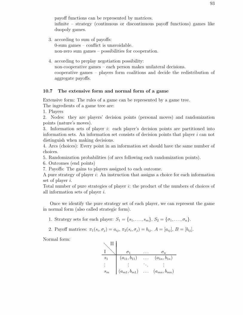
93
payoff functions can be represented by matrices.infinite – strategy (continuous or discontinuous payoff functions) games likeduopoly games.
3. according to sum of payoffs:0-sum games – conflict is unavoidable.non-zero sum games – possibilities for cooperation.
4. according to preplay negotiation possibility:non-cooperative games – each person makes unilateral decisions.cooperative games – players form coalitions and decide the redistribution ofaggregate payoffs.
10.7 The extensive form and normal form of a game
Extensive form: The rules of a game can be represented by a game tree.The ingredients of a game tree are:1. Players2. Nodes: they are players’ decision points (personal moves) and randomizationpoints (nature’s moves).3. Information sets of player i: each player’s decision points are partitioned intoinformation sets. An information set consists of decision points that player i can notdistinguish when making decisions.4. Arcs (choices): Every point in an information set should have the same number ofchoices.5. Randomization probabilities (of arcs following each randomization points).6. Outcomes (end points)7. Payoffs: The gains to players assigned to each outcome.A pure strategy of player i: An instruction that assigns a choice for each informationset of player i.Total number of pure strategies of player i: the product of the numbers of choices ofall information sets of player i.
Once we identify the pure strategy set of each player, we can represent the gamein normal form (also called strategic form).
1. Strategy sets for each player: S1 = {s1, . . . , sm}, S2 = {σ1, . . . , σn}.
2. Payoff matrices: π1(si, σj) = aij , π2(si, σj) = bij . A = [aij ], B = [bij ].
Normal form:II
I @@
@
σ1 . . . σn
s1 (a11, b11) . . . (a1n, b1n)...
.... . .
...sm (am1, bm1) . . . (amn, bmn)
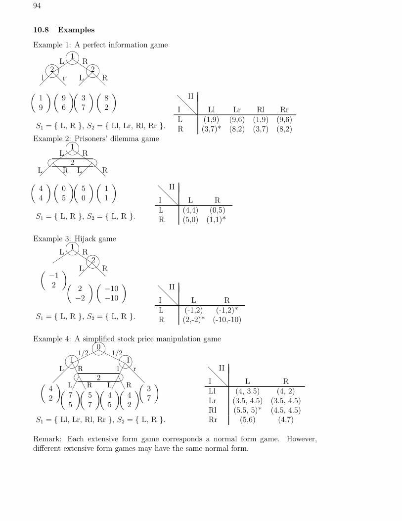
94
10.8 Examples
Example 1: A perfect information game
��
�Q
QQ����1
L R
��
@@����2
l r ��
@@����2
L R
(
19
)(
96
)(
37
)(
82
)
S1 = { L, R }, S2 = { Ll, Lr, Rl, Rr }.
II
I @@
@
Ll Lr Rl RrL (1,9) (9,6) (1,9) (9,6)R (3,7)* (8,2) (3,7) (8,2)
Example 2: Prisoners’ dilemma game
��
�Q
QQ����1
L R
��
@@
��
@@
� �2L R L R
(
44
)(
05
)(
50
)(
11
)
S1 = { L, R }, S2 = { L, R }.
II
I @@
@
L RL (4,4) (0,5)R (5,0) (1,1)*
Example 3: Hijack game
��
�Q
QQ����1
L R
��
@@����
2L R
(
−12
)
(
2−2
)(
−10−10
)
S1 = { L, R }, S2 = { L, R }.
II
I @@
@
L RL (-1,2) (-1,2)*R (2,-2)* (-10,-10)
Example 4: A simplified stock price manipulation game
����
HHHH����0
1/2 1/2
��
�
AA����1
L R ��
@@
@
����
1l r
��
AA
��
AA
� �2L R L R(
42
)
(
75
)(
57
)(
45
)(
42
)
(
37
)
S1 = { Ll, Lr, Rl, Rr }, S2 = { L, R }.
II
I @@
@
L RLl (4, 3.5) (4, 2)Lr (3.5, 4.5) (3.5, 4.5)Rl (5.5, 5)* (4.5, 4.5)Rr (5,6) (4,7)
Remark: Each extensive form game corresponds a normal form game. However,different extensive form games may have the same normal form.
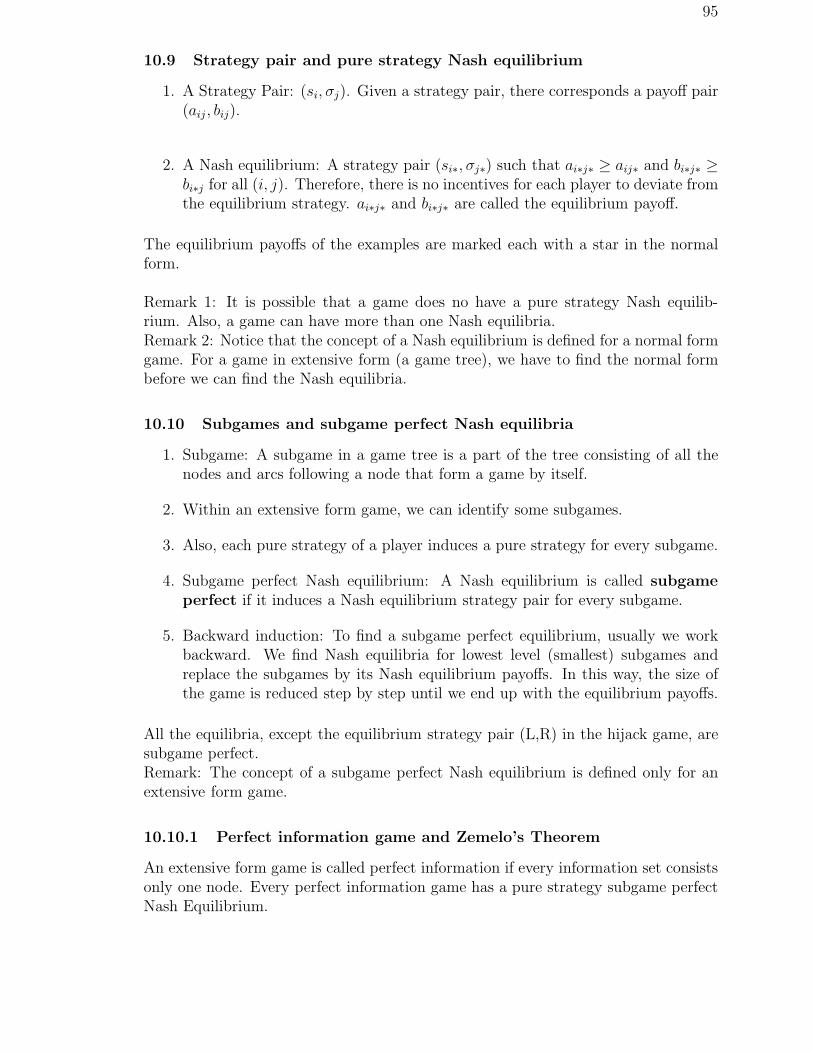
95
10.9 Strategy pair and pure strategy Nash equilibrium
1. A Strategy Pair: (si, σj). Given a strategy pair, there corresponds a payoff pair(aij , bij).
2. A Nash equilibrium: A strategy pair (si∗, σj∗) such that ai∗j∗ ≥ aij∗ and bi∗j∗ ≥bi∗j for all (i, j). Therefore, there is no incentives for each player to deviate fromthe equilibrium strategy. ai∗j∗ and bi∗j∗ are called the equilibrium payoff.
The equilibrium payoffs of the examples are marked each with a star in the normalform.
Remark 1: It is possible that a game does no have a pure strategy Nash equilib-rium. Also, a game can have more than one Nash equilibria.Remark 2: Notice that the concept of a Nash equilibrium is defined for a normal formgame. For a game in extensive form (a game tree), we have to find the normal formbefore we can find the Nash equilibria.
10.10 Subgames and subgame perfect Nash equilibria
1. Subgame: A subgame in a game tree is a part of the tree consisting of all thenodes and arcs following a node that form a game by itself.
2. Within an extensive form game, we can identify some subgames.
3. Also, each pure strategy of a player induces a pure strategy for every subgame.
4. Subgame perfect Nash equilibrium: A Nash equilibrium is called subgameperfect if it induces a Nash equilibrium strategy pair for every subgame.
5. Backward induction: To find a subgame perfect equilibrium, usually we workbackward. We find Nash equilibria for lowest level (smallest) subgames andreplace the subgames by its Nash equilibrium payoffs. In this way, the size ofthe game is reduced step by step until we end up with the equilibrium payoffs.
All the equilibria, except the equilibrium strategy pair (L,R) in the hijack game, aresubgame perfect.Remark: The concept of a subgame perfect Nash equilibrium is defined only for anextensive form game.
10.10.1 Perfect information game and Zemelo’s Theorem
An extensive form game is called perfect information if every information set consistsonly one node. Every perfect information game has a pure strategy subgame perfectNash Equilibrium.
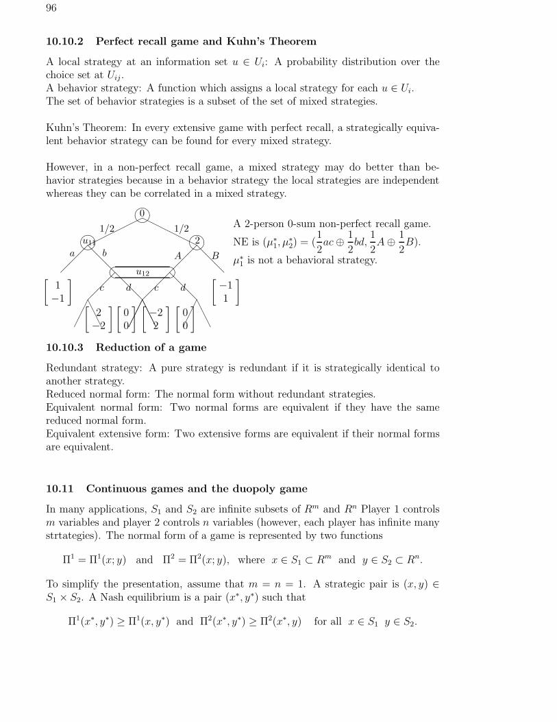
96
10.10.2 Perfect recall game and Kuhn’s Theorem
A local strategy at an information set u ∈ Ui: A probability distribution over thechoice set at Uij .A behavior strategy: A function which assigns a local strategy for each u ∈ Ui.The set of behavior strategies is a subset of the set of mixed strategies.
Kuhn’s Theorem: In every extensive game with perfect recall, a strategically equiva-lent behavior strategy can be found for every mixed strategy.
However, in a non-perfect recall game, a mixed strategy may do better than be-havior strategies because in a behavior strategy the local strategies are independentwhereas they can be correlated in a mixed strategy.
������
HHHHHH�
��
@@
@
��
�
@@
@�
��
@@
@�
��
AAA
��
�
AAA
��
�
@@
@�
��
AAA
��
�
AAA
� ��0� ��u11 � ��2� �u12
1/2 1/2
a b A B
c d c d
[
1−1
] [
−11
]
[
2−2
][
00
] [
−22
] [
00
]
A 2-person 0-sum non-perfect recall game.
NE is (µ∗1, µ
∗2) = (
1
2ac⊕ 1
2bd,
1
2A⊕ 1
2B).
µ∗1 is not a behavioral strategy.
10.10.3 Reduction of a game
Redundant strategy: A pure strategy is redundant if it is strategically identical toanother strategy.Reduced normal form: The normal form without redundant strategies.Equivalent normal form: Two normal forms are equivalent if they have the samereduced normal form.Equivalent extensive form: Two extensive forms are equivalent if their normal formsare equivalent.
10.11 Continuous games and the duopoly game
In many applications, S1 and S2 are infinite subsets of Rm and Rn Player 1 controlsm variables and player 2 controls n variables (however, each player has infinite manystrtategies). The normal form of a game is represented by two functions
Π1 = Π1(x; y) and Π2 = Π2(x; y), where x ∈ S1 ⊂ Rm and y ∈ S2 ⊂ Rn.
To simplify the presentation, assume that m = n = 1. A strategic pair is (x, y) ∈S1 × S2. A Nash equilibrium is a pair (x∗, y∗) such that
Π1(x∗, y∗) ≥ Π1(x, y∗) and Π2(x∗, y∗) ≥ Π2(x∗, y) for all x ∈ S1 y ∈ S2.

97
Consider the case when Πi are continuously differentiable and Π1 is strictly concavein x and Π2 strictly concave in y (so that we do not have to worry about the SOC’s).
Reaction functions and Nash equilibrium:To player 1, x is his endogenous variable and y is his exogenous variable. For each ychosen by player 2, player 1 will choose a x ∈ S1 to maximize his objective functionΠ1. This relationship defines a behavioral equation x = R1(y) which can be obtainedby solving the FOC for player 1, Π1
x(x; y) = 0. Similarly, player 2 regards y as en-dogenous and x exogenous and wants to maximize Π2 for a given x chosen by player1. Player 2’s reaction function (behavioral equation) y = R2(x) is obtained by solvingΠ2
y(x; y) = 0. A Nash equilibrium is an intersection of the two reaction functions.The FOC for a Nash equilibrium is given by Π1
x(x∗; y∗) = 0 and Π2
y(x∗; y∗) = 0.
Duopoly game:There are two sellers (firm 1 and firm 2) of a product.The (inverse) market demand function is P = a−Q.The marginal production costs are c1 and c2, respectively.Assume that each firm regards the other firm’s output as given (not affected by hisoutput quantity).The situation defines a 2-person game as follows: Each firm i controls his own outputquantity qi. (q1, q2) together determine the market price P = a− (q1 + q2) which inturn determines the profit of each firm:
Π1(q1, q2) = (P−c1)q1 = (a−c1−q1−q2)q1 and Π2(q1, q2) = (P−c2)q2 = (a−c2−q1−q2)q2
The FOC are ∂Π1/∂q1 = a− c1 − q2 − 2q1 = 0 and ∂Π2/∂q2 = a− c2 − q1 − 2q2 = 0.The reaction functions are q1 = 0.5(a− c1 − q2) and q2 = 0.5(a− c2 − q1).The Cournot Nash equilibrium is (q∗1 , q
∗2) = ((a− 2c1 + c2)/3, (a− 2c2 + c1)/3) with
P ∗ = (a + c1 + c2)/3. (We have to assume that a− 2c1 + c2, a− 2c2 + c1 ≥ 0.)
10.11.1 A simple bargaining model
Two players, John and Paul, have $ 1 to divide between them. They agree to spendat most two days negotiating over the division. The first day, John will make an offer,Paul either accepts or comes back with a counteroffer the second day. If they cannotreach an agreement in two days, both players get zero. John (Paul) discounts payoffsin the future at a rate of α (β) per day.
A subgame perfect equilibrium of this bargaining game can be derived using back-ward induction.1. On the second day, John would accept any non-negative counteroffer made byPaul. Therefore, Paul would make proposal of getting the whole $ 1 himself and Johnwould get $ 0.2. On the first day, John should make an offer such that Paul gets an amount equiv-alent to getting $ 1 the second day, otherwise Paul will reject the offer. Therefore,John will propose of 1− β for himself and β for Paul and Paul will accept the offer.
98
An example of a subgame non-perfect Nash equilibrium is that John proposes ofgetting 1-0.5β for himself and 0.5β for Paul and refuses to accept any counteroffermade by Paul. In this equilibrium, Paul is threatened by John’s incredible threat andaccepts only one half of what he should have had in a perfect equilibrium.
10.12 2-person 0-sum game
1. B = −A so that aij + bij = 0.
2. Maxmin strategy: If player 1 plays si, then the minimum he will have is minj aij ,called the security level of strategy si. A possible guideline for player 1 is tochoose a strategy such that the security level is maximized: Player 1 choosessi∗ so that minj ai∗j ≥ minj aij for all i. Similarly, since bij = −aij , Player 2chooses σj∗ so that maxi aij∗ ≤ maxi aij for all j.
3. Saddle point: If ai∗j∗ = maxi minj aij = minj maxi aij, then (si∗, σj∗) is called asaddle point. If a saddle point exists, then it is a Nash equilibrium.
A1 =
(
2 1 4−1 0 6
)
A2 =
(
1 00 1
)
In example A1, maxi minj aij = minj maxi aij = 1 (s1, σ2) is a saddle point andhence a Nash equilibrium. In A2, maxi minj aij = 0 6= minj maxi aij = 1 and nosaddle point exists. If there is no saddle points, then there is no pure strategyequilibrium.
4. Mixed strategy for player i: A probability distribution over Si. p = (p1, . . . , pm),q = (q1, . . . , qn)′. (p, q) is a mixed strategy pair. Given (p, q), the expectedpayoff of player 1 is pAq. A mixed strategy Nash equilibrium (p∗, q∗) is suchthat p∗Aq∗ ≥ pAq∗ and p∗Aq∗ ≤ p∗Aq for all p and all q.
5. Security level of a mixed strategy: Given player 1’s strategy p, there is a purestrategy of player 2 so that the expected payoff to player 1 is minimized, justas in the case of a pure strategy of player 1.
t(p) ≡ minj{∑
i
piai1, . . . ,∑
i
piain}.
The problem of finding the maxmin mixed strategy (to find p∗ to maximizet(p)) can be stated as
maxp
t subj. to∑
i
piai1 ≥ t, . . . ,∑
i
piain ≥ t,∑
i
pi = 1.
6. Linear programming problem: The above problem can be transformed into alinear programming problem as follows: (a) Add a positive constant to eachelement of A to insure that t(p) > 0 for all p. (b) Define yi ≡ pi/t(p) and
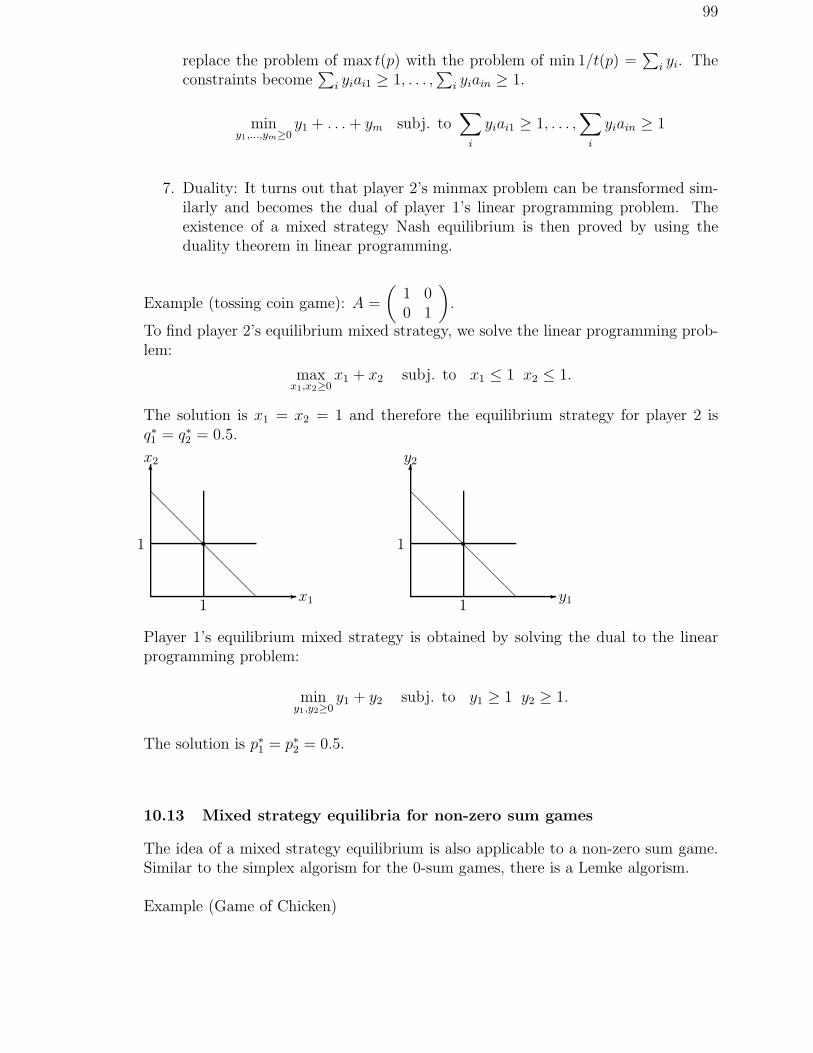
99
replace the problem of max t(p) with the problem of min 1/t(p) =∑
i yi. Theconstraints become
∑
i yiai1 ≥ 1, . . . ,∑
i yiain ≥ 1.
miny1,...,ym≥0
y1 + . . . + ym subj. to∑
i
yiai1 ≥ 1, . . . ,∑
i
yiain ≥ 1
7. Duality: It turns out that player 2’s minmax problem can be transformed sim-ilarly and becomes the dual of player 1’s linear programming problem. Theexistence of a mixed strategy Nash equilibrium is then proved by using theduality theorem in linear programming.
Example (tossing coin game): A =
(
1 00 1
)
.
To find player 2’s equilibrium mixed strategy, we solve the linear programming prob-lem:
maxx1,x2≥0
x1 + x2 subj. to x1 ≤ 1 x2 ≤ 1.
The solution is x1 = x2 = 1 and therefore the equilibrium strategy for player 2 isq∗1 = q∗2 = 0.5.
-x1
6x2
@@
@@
@@
@@
1
1 r- y1
6y2
@@
@@
@@
@@
1
1 r
Player 1’s equilibrium mixed strategy is obtained by solving the dual to the linearprogramming problem:
miny1,y2≥0
y1 + y2 subj. to y1 ≥ 1 y2 ≥ 1.
The solution is p∗1 = p∗2 = 0.5.
10.13 Mixed strategy equilibria for non-zero sum games
The idea of a mixed strategy equilibrium is also applicable to a non-zero sum game.Similar to the simplex algorism for the 0-sum games, there is a Lemke algorism.
Example (Game of Chicken)
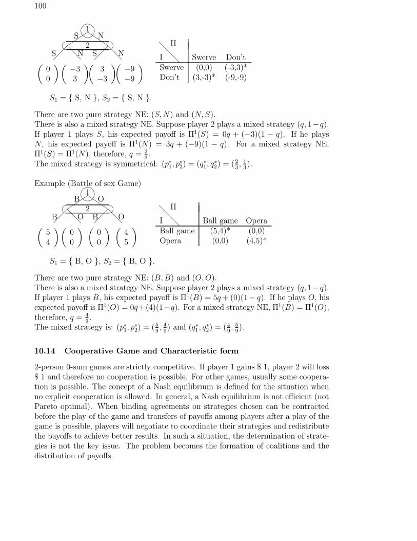
100
��
�Q
QQ����1
S N
��
@@
��
@@
� �2S N S N
(
00
)(
−33
)(
3−3
)(
−9−9
)
S1 = { S, N }, S2 = { S, N }.
II
I @@
@
Swerve Don’tSwerve (0,0) (-3,3)*Don’t (3,-3)* (-9,-9)
There are two pure strategy NE: (S, N) and (N, S).There is also a mixed strategy NE. Suppose player 2 plays a mixed strategy (q, 1−q).If player 1 plays S, his expected payoff is Π1(S) = 0q + (−3)(1 − q). If he playsN , his expected payoff is Π1(N) = 3q + (−9)(1 − q). For a mixed strategy NE,Π1(S) = Π1(N), therefore, q = 2
3.
The mixed strategy is symmetrical: (p∗1, p∗2) = (q∗1, q
∗2) = (2
3, 1
3).
Example (Battle of sex Game)
��
�Q
QQ����1
B O
��
@@
��
@@
� �2B O B O
(
54
)(
00
) (
00
) (
45
)
S1 = { B, O }, S2 = { B, O }.
II
I @@
@
Ball game OperaBall game (5,4)* (0,0)Opera (0,0) (4,5)*
There are two pure strategy NE: (B, B) and (O, O).There is also a mixed strategy NE. Suppose player 2 plays a mixed strategy (q, 1−q).If player 1 plays B, his expected payoff is Π1(B) = 5q + (0)(1− q). If he plays O, hisexpected payoff is Π1(O) = 0q+(4)(1−q). For a mixed strategy NE, Π1(B) = Π1(O),therefore, q = 4
9.
The mixed strategy is: (p∗1, p∗2) = (5
9, 4
9) and (q∗1 , q
∗2) = (4
9, 5
9).
10.14 Cooperative Game and Characteristic form
2-person 0-sum games are strictly competitive. If player 1 gains $ 1, player 2 will loss$ 1 and therefore no cooperation is possible. For other games, usually some coopera-tion is possible. The concept of a Nash equilibrium is defined for the situation whenno explicit cooperation is allowed. In general, a Nash equilibrium is not efficient (notPareto optimal). When binding agreements on strategies chosen can be contractedbefore the play of the game and transfers of payoffs among players after a play of thegame is possible, players will negotiate to coordinate their strategies and redistributethe payoffs to achieve better results. In such a situation, the determination of strate-gies is not the key issue. The problem becomes the formation of coalitions and thedistribution of payoffs.

101
Characteristic form of a game:The player set: N = {1, 2, . . . , n}.A coalition is a subset of N : S ⊂ N .A characteristic function v specifies the maximum total payoff of each coalition.Consider the case of a 3-person game. There are 8 subsets of N = {1, 2, 3}, namely,φ, (1), (2), (3), (12), (13), (23), (123).Therefore, a characteristic form game is determined by 8 values v(φ), v(1), v(2), v(3), v(12), v(13), v(23Super-additivity: If A ∩B = φ, then v(A ∪ B) ≥ v(A) + v(B).An imputation is a payoff distribution (x1, x2, x3).Individual rationality: xi ≥ v(i).Group rationality:
∑
i∈S xi ≥ v(S).Core C: the set of imputations that satisfy individual rationality and group rational-ity for all S.
Marginal contribution of player i in a coalition S ∪ i: v(S ∪ i)− v(S)Shapley value of player i is an weighted average of all marginal contributions
πi =∑
S⊂N
|S|!(n− |S| − 1)!
n![v(S ∪ i)− v(S)].
Example: v(φ) = v(1) = v(2) = v(3) = 0, v(12) = v(13) = v(23) = 0.5, v(123) = 1.C = {(x1, x2, x3), xi ≥ 0, xi + xj ≥ 0.5, x1 + x2 + x3 = 1}. Both (0.3, 0.3, 0.4) and(0.2, 0.4, 0.4) are in C.The Shapley values are (π1, π2, π3) = (1
3, 1
3, 1
3).
Remark 1: The core of a game can be empty. However, the Shapley values areuniquely determined.Remark 2: Another related concept is the von-Neumann Morgenstern solution. SeeCH 6 of Intriligator’s Mathematical Optimization and Economic Theory for the mo-tivations of these concepts.
10.15 The Nash bargaining solution for a nontransferable 2-person coop-erative game
In a nontransferable cooperative game, after-play redistributions of payoffs are im-possible and therefore the concepts of core and Shapley values are not suitable. Forthe case of 2-person games, the concept of Nash bargaining solutions are useful.Let F ⊂ R2 be the feasible set of payoffs if the two players can reach an agreementand Ti the payoff of player i if the negotiation breaks down. Ti is called the threatpoint of player i. The Nash bargaining solution (x∗
1, x∗2) is defined to be the solution
to the following problem:

102
-x1
6x2
T1
T2
x∗1
x∗2
max(x1,x2)∈F
(x1 − T1)(x2 − T2)
See CH 6 of Intriligator’s book for the motivations of the solution concept.
10.16 Problems
1. Consider the following two-person 0-sum game:I \ II σ1 σ2 σ3
s1 4 3 -2s2 3 4 10s3 7 6 8
(a) Find the max min strategy of player I smaxmin and the min max strategyof player II σmin max.
(b) Is the strategy pair (smaxmin, σmin max) a Nash equilibrium of the game?
(c) What are the equilibrium payoffs?
2. Find the maxmin strategy (smaxmin) and the minmax strategy (σmin max) of thefollowing two-person 0-sum game:
I \ II σ1 σ2
s1 -3 6s2 8 -2s3 6 3
Is the strategy pair (smaxmin, σmin max) a Nash equilibrium? If not, use simplexmethod to find the mixed strategy Nash equilibrium.
3. Find the (mixed strategy) Nash Equilibrium of the following two-person game:I \ II H T
H (-2, 2) (2, -1)T (2, -2) (-1,2)
4. Suppose that two firms producing a homogenous product face a linear demandcurve P = a−bQ = a−b(q1+q2) and that both have the same constant marginalcosts c. For a given quantity pair (q1, q2), the profits are Πi = qi(P − c) =qi(a − bq1 − bq2 − c), i = 1, 2. Find the Cournot Nash equilibrium output ofeach firm.
5. Suppose that in a two-person cooperative game without side payments, if thetwo players reach an agreement, they can get (Π1, Π2) such that Π2
1 + Π2 = 47

103
and if no agreement is reached, player 1 will get T1 = 3 and player 2 will getT2 = 2.
(a) Find the Nash solution of the game.
(b) Do the same for the case when side payments are possible. Also answerhow the side payments should be done?
6. A singer (player 1), a pianist (player 2), and a drummer (player 3) are offered$ 1,000 to play together by a night club owner. The owner would alternativelypay $ 800 the singer-piano duo, $ 650 the piano drums duo, and $ 300 the pianoalone. The night club is not interested in any other combination. Howeover,the singer-drums duo makes $ 500 and the singer alone gets $ 200 a night in arestaurant. The drums alone can make no profit.
(a) Write down the characteristic form of the cooperative game with side pay-ments.
(b) Find the Shapley values of the game.
(c) Characterize the core.