Lecture notes on Geometric Group Theory

Under construction

Alessandro Sisto

July 3, 2014

Contents

1 Foreword 4

I Cayley graphs, quasi-isometries and Milnor-Svarc 5

2 The Cayley graph 62.1 Metric graphs . . . . . . . . . . . . . . . . . . . . . . . . . . . . . 62.2 Definition and examples . . . . . . . . . . . . . . . . . . . . . . . 7

2.2.1 Examples . . . . . . . . . . . . . . . . . . . . . . . . . . . 82.3 G acts on the Cayley graph . . . . . . . . . . . . . . . . . . . . . 92.4 Cay(G,S) is nice . . . . . . . . . . . . . . . . . . . . . . . . . . . 10

2.4.1 Geodesic metric spaces . . . . . . . . . . . . . . . . . . . . 102.4.2 Back to Cayley graphs . . . . . . . . . . . . . . . . . . . . 12

2.5 The action of G is nice . . . . . . . . . . . . . . . . . . . . . . . . 132.6 A relaxing exercise . . . . . . . . . . . . . . . . . . . . . . . . . . 13

3 Quasi-isometries 153.0.1 Examples . . . . . . . . . . . . . . . . . . . . . . . . . . . 163.0.2 Quasi-inverses . . . . . . . . . . . . . . . . . . . . . . . . . 163.0.3 Cayley graphs and quasi-isometries . . . . . . . . . . . . . 183.0.4 Quasi-isometric groups and (un)distorted subgroups . . . 18

3.1 The final exercise . . . . . . . . . . . . . . . . . . . . . . . . . . . 20

4 Milnor-Svarc Lemma 214.1 A digression on growth . . . . . . . . . . . . . . . . . . . . . . . . 23

II Hyperbolic spaces and groups 26

5 Definition, examples and quasi-isometry invariance 275.1 Examples (for the moment!) . . . . . . . . . . . . . . . . . . . . . 285.2 Non-examples . . . . . . . . . . . . . . . . . . . . . . . . . . . . . 295.3 List of properties . . . . . . . . . . . . . . . . . . . . . . . . . . . 305.4 Quasi-isometry invariance . . . . . . . . . . . . . . . . . . . . . . 30

5.4.1 Proof of Proposition 5.4.2 . . . . . . . . . . . . . . . . . . 32

1

6 Hn 356.1 Two models . . . . . . . . . . . . . . . . . . . . . . . . . . . . . . 356.2 Lots of isometries! . . . . . . . . . . . . . . . . . . . . . . . . . . 36

6.2.1 In the half-plane model . . . . . . . . . . . . . . . . . . . 366.2.2 In the disk model . . . . . . . . . . . . . . . . . . . . . . . 37

6.3 Geodesics and hyperbolicity . . . . . . . . . . . . . . . . . . . . . 376.3.1 Hyperbolicity . . . . . . . . . . . . . . . . . . . . . . . . . 38

6.4 Right-angled n-gons and hyperbolic surfaces . . . . . . . . . . . . 38

7 Commuting stuff in hyperbolic groups 417.1 Results . . . . . . . . . . . . . . . . . . . . . . . . . . . . . . . . . 427.2 Proof of Theorem 7.1.1 . . . . . . . . . . . . . . . . . . . . . . . . 43

8 Geometry of presentations 488.1 The algebraic point of view . . . . . . . . . . . . . . . . . . . . . 498.2 Finite presentations . . . . . . . . . . . . . . . . . . . . . . . . . 518.3 Finite presentations of hyperbolic groups and Dehn functions . . 53

9 Small cancellation 569.1 Examples 1,2,... . . . . . . . . . . . . . . . . . . . . . . . . . . . . 579.2 Proof of Theorem 9.0.8 . . . . . . . . . . . . . . . . . . . . . . . . 589.3 ... and 3 . . . . . . . . . . . . . . . . . . . . . . . . . . . . . . . . 61

10 Free subgroups 63

III CAT(0) spaces and cube complexes 64

11 CAT(0) geometry 6511.1 The CAT(0) inequality . . . . . . . . . . . . . . . . . . . . . . . . 6511.2 First examples . . . . . . . . . . . . . . . . . . . . . . . . . . . . 6611.3 Some properties . . . . . . . . . . . . . . . . . . . . . . . . . . . . 6711.4 Groups acting on CAT(0) spaces . . . . . . . . . . . . . . . . . . 6911.5 Connections with hyperbolicity . . . . . . . . . . . . . . . . . . . 7011.6 Nonpositively curved complexes . . . . . . . . . . . . . . . . . . . 71

12 CAT(0) cube complexes 7412.1 Definitions, nonpositive curvature and flag links . . . . . . . . . . 7412.2 First examples . . . . . . . . . . . . . . . . . . . . . . . . . . . . 7612.3 Right-angled Artin groups... . . . . . . . . . . . . . . . . . . . . . 77

12.3.1 Salvetti complex . . . . . . . . . . . . . . . . . . . . . . . 7812.4 ... and their subgroups . . . . . . . . . . . . . . . . . . . . . . . . 7912.5 Special cube complexes . . . . . . . . . . . . . . . . . . . . . . . 80

2

13 Cubulation 8313.1 Properties of hyperplanes . . . . . . . . . . . . . . . . . . . . . . 8313.2 From walls to cube complexes . . . . . . . . . . . . . . . . . . . . 8413.3 Examples . . . . . . . . . . . . . . . . . . . . . . . . . . . . . . . 86

3

Chapter 1

Foreword

These are lecture notes for the 2014 course on Geometric Group Theory at ETHZurich.

Geometric Group Theory is the art of studying groups without using algebra.Here’s a rather effective description from Ric Wade:

[Geometric Group Theory] is about using geometry (i.e. drawing pictures)to help us understand groups, which can otherwise be fairly dry algebraic objects(i.e. a bunch of letters on a piece of paper).

The way to use geometry to study groups is considering their (isometric)actions on metric spaces. Many theorems in Geometric Group Theory look like:Let G be a group acting “nicely” on a “nice” space. Then G ...

The core part of the course is devoted to (Gromov-)hyperbolic spaces andgroups.

I’m experimenting a bit with the style. What I want to do is explainingconcepts, ideas, etc. in a way that resembles how you would explain them inperson more than a traditional book/ set of lecture notes. “Traditional” booksand lecture notes about Geometric Group Theory or hyperbolic groups includethe following:

• A course on geometric group theory, by Bowditch

• Metric spaces of non-positive curvature, by Bridson and Haefliger

• Les groupes hyperboliques de Gromov, by Coornaert, Delzant and Pa-padopoulos

• Sur les groupes hyperboliques d’apres Mikhael Gromov, by Ghys and de laHarpe

The references will all be given at the end.

4

Part I

Cayley graphs,quasi-isometries and

Milnor-Svarc

5

Chapter 2

The Cayley graph

The aim of this chapter is to introduce a metric space called Cayley graph thatcan be naturally associated to a finitely generated group (together with a fixedfinite generating set). The group acts on its the Cayley graph in a natural way.

Notation: In this chapter G will always denote a group generated by thefinite set S ⊆ G\{1}. For convenience we also assume S = S−1 = {s−1|s ∈ S}.

There’s no deep reason to require 1 /∈ S, but there are a few points whereallowing 1 as a generator makes things more annoying to write down. RequiringS = S−1 is also not very important but sometimes convenient.

2.1 Metric graphs

This section can be safely skipped if you know what a metric graph is. Or evenif you can just guess it.

Recall that a graph Γ consists of points called vertices and copies of [0, 1]connecting pairs of vertices called edges. Also, interiors of distinct edges aredisjoint. (Sometimes one requires that there are no double edges, but we don’tneed to.)

Suppose that we assigned to each edge e of a given connected graph Γ somepositive number l(e) (its length). Then we can define on Γ a pseudo-metric,which we now describe in two ways.

If we regard each edge as an isometric copy of [0, l(e)], we have a naturalway of defining the length of a path consisting of the concatenation of finitelymany subpaths of edges. We can then define the “distance” d(x, y) betweentwo points x, y ∈ Γ to just be the infimum of the lengths of paths as aboveconnecting them. This infimum might be 0, and this is the only reason why dmay fail to define a metric. The infimum is never 0 for x 6= y if there is a lowerbound on the length of the edges.

Here is another way to describe d. For each edge e fix a homeomorphismφe : e → [0, 1] as in the definition of edge. Define the auxiliary function ρ

6

in the following way. If x, y belong to the same edge e, then define ρ(x, y) =l(e)|φe(x)− φe(y)|, and set ρ(x, y) = +∞ otherwise. Finally, set

d(x, y) = infx=x0,...,xn=y

∑ρ(xi, xi+1).

{xi} as above is usually called chain (from x to y).

Lemma 2.1.1. In the definition one can equivalently only take chains x =x0, . . . , xn = y with the additional constraint that xi is a vertex for i 6= 0, n.

Proof. If∑ρ(xi, xi+1) is finite then for any xi which is not a vertex both xi−1

and xi+1 have to be contained in the same edge as xi, if i 6= 0, n. Removing xifrom the chain does not increase the value of the sum because ρ(xi−1, xi+1) ≤ρ(xi−1, xi)+ρ(xi, xi+1) by triangular inequality. Hence, starting from any chain,we can iteratively remove the non-vertices in the “middle” part and find anew chain {yi} satisfying our extra requirement and so that

∑ρ(yi, yi+1) ≤∑

ρ(xi, xi+1). Hence, the infimum taken over the smaller set of chains that weare considering coincides with the the infimum over all chains from x to y.

We will mostly use edges of length 1, but occasionally edges of differentlengths will also show up.

2.2 Definition and examples

Here is the definition of Cayley graph.

Definition 2.2.1. The Cayley graph Cay(G,S) of G with respect to S is themetric graph with

1. vertex set G,

2. an edge connecting g, h ∈ G if and only if g−1h ∈ S, i.e. if and only ifthere exists s ∈ S with h = gs,

3. all edges of length 1.

We denote the metric on Cay(G,S) as dS .

7

2.2.1 Examples

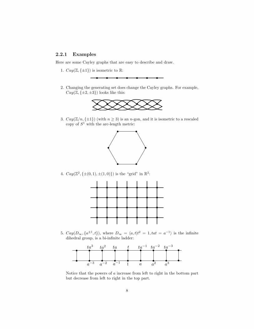
Here are some Cayley graphs that are easy to describe and draw.

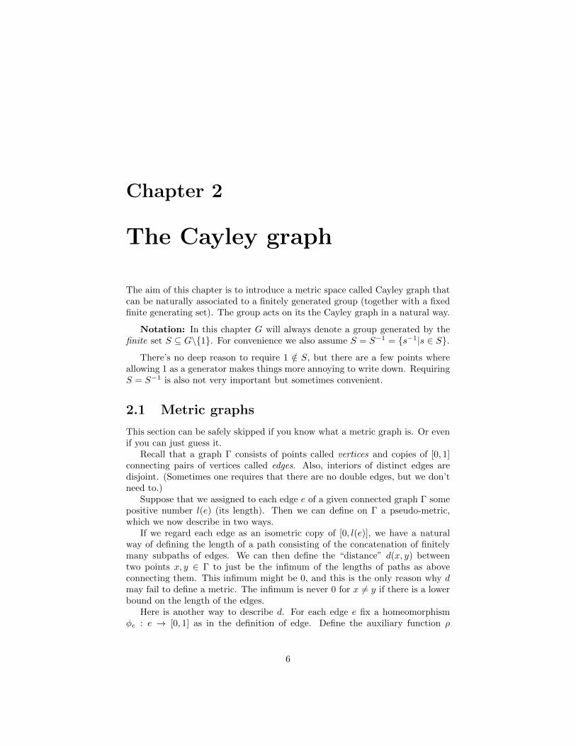
1. Cay(Z, {±1}) is isometric to R:

2. Changing the generating set does change the Cayley graphs. For example,Cay(Z, {±2,±3}) looks like this:

3. Cay(Z/n, {±1}) (with n ≥ 3) is an n-gon, and it is isometric to a rescaledcopy of S1 with the arc-length metric:

4. Cay(Z2, {±(0, 1),±(1, 0)}) is the “grid” in R2:

5. Cay(D∞, {a±1, t}), where D∞ = 〈a, t|t2 = 1, tat = a−1〉 is the infinitedihedral group, is a bi-infinite ladder:

Notice that the powers of a increase from left to right in the bottom partbut decrease from left to right in the top part.

8

6. Cay(F2, {a±1, b±1}) (where a, b are a basis of the free group on two gen-erators F2) is what’s called a tree and looks like this:

In the rest of this chapter we will explore the properties of Cayley graphs.Here is the first one.

Fact 1: For g, h ∈ G, we have dS(g, h) = min{n|∃s1, . . . , sn g−1h =s1 . . . sn} (and dS(g, h) = 0 if g = h).

In words, the distance between g and h is the minimum length of a wordin the alphabet S representing g−1h, i.e. the word length of g−1h. One oftendenotes dS(1, g) by |g|S .

Fact 1 follows directly from Lemma 2.1.1.

2.3 G acts on the Cayley graph

Fact 2: G acts by isometries on Cay(G,S). Such action extends the action ofG on itself by left translation (i.e. g(h) = gh).

In order to convince ourselves of Fact 2 notice that, for any g, h1, h2 ∈ G,there is an edge from h1 to h2 if and only if there is an edge between gh1 andgh2. This is just because (gh1)−1gh2 = h−1

1 h2. If you prefer (I do), if youobtain h2 from h1 by multiplying on the right by some s ∈ S, i.e. h2 = h1s,then clearly you also obtain gh2 from gh1 multiplying on the right by the sames.

Now, using the observation above we can extend the left multiplication byg ∈ G across the edges of the Cayley graph.

More formally, in order to define an action by isometries of G on Cay(G,S)one has to assign to each g ∈ G an isometry φg. Such isometry can be writ-ten down as follows. For x ∈ G, φg(x) is just gx. For x on the edge from,say, h1 to h2, φg(x) is the only point on the edge from gh1 to gh2 satisfyingdS(gh1, φg(x)) = dS(h1, x).

The following properties have to be checked for g 7→ φg to define an actionby isometries, and they are both straightforward.

1. φg is an isometry,

9

2. φgh = φg ◦ φh.

From now on, for notational convenience we will write g instead of φg, thatis to say, if you like, we identify the group element g with its induced isometryon the Cayley graph.

Don’t read this, it’s not worth it:

What we just defined is a left action, meaning that g → φg is a homomorphism from G to the isometry group

of Cay(G, S) IF composition in the said isometry group is defined right-to-left, i.e. (i1 ◦ i2)(x) = i1(i2(x)) for all

isometries i1, i2 and x ∈ Cay(G, S).

2.4 Cay(G,S) is nice

In this section we address the question: How good is Cay(G,S) as a metricspace?

Here is the first good property of Cayley graphs.

Fact 3: Cay(G,S) is a proper metric space, i.e. its closed balls are compact.

Fact 3 is just a consequence of the fact that any ball, say of integer radius,is the union of finitely many edges, and each edge is compact.

Exercise: How many edges can there be at most in a ball of radius n (interms of the cardinality of S)? What is a pair (group, generating set) wheresuch number of edges is maximal?

You may have noticed that up to now edges have just been an annoyance,and we would have been better off just putting the metric as in Fact 1 on G.But fear not, we are about to use them.

Fact 4: Cay(G,S) is a geodesic metric space.

You can skip the next subsection if you already know what this means.

2.4.1 Geodesic metric spaces

Let us fix a metric space X from now until the end of the subsection.For α a path in X (i.e. a continuous map α : [0, 1] → X), let us define the

length of α as

l(α) = sup0=t0≤···≤tn=1

∑d(α(ti), α(ti+1)).

The idea is rather simple. Suppose you want to formally define the notion oflength of a path. One property you would like is that if you approximate yourcurve by a concatenation of “straight lines” then the length of such concatena-tion approximates the length of the path (well, if the path has finite length).The length of a “straight line” should be the same as the distance between theendpoints, whence the definition above.

Two further properties you would like are content of the following two re-marks.

10

Remark 2.4.1. For any path α, we have l(α) ≥ d(α(0), α(1)). In fact, the sumsappearing in the definition of length are all greater or equal than d(α(0), α(1))by triangular inequality (and induction).

Remark 2.4.2. Let us denote the concatenation of the paths α, β by α∗β. Thenl(α ∗ β) = l(α) + l(β). To prove the inequality ≤, just notice that given a chainof points “approximating” α and one “approximating” β, we can concatenatethem and form a chain of points for α∗β. To prove ≥, notice that given a chainof points “approximating” α∗β we can add a point and make it a concatenationof chains for α and β. If this sounds mysterious, it’s probably a good idea towork out the details yourself.

We mentioned “straight lines” above. They are actually called geodesics:

Definition 2.4.3. The path α is a geodesic if l(α) = d(α(0), α(1)). The metricspace X is geodesic if for any pair of points of X there is a geodesic connectingthem.

Hence, geodesics are the most efficient paths to get between two points. Weconclude the subsection with two useful properties of geodesics.

Proposition 2.4.4. 1. A subpath of a geodesic is a geodesic.

2. if α is a geodesic then for any s ≤ t ≤ u we have

d(α(s), α(t)) + d(α(t), α(u)) = d(α(s), α(u)).

The idea behind the first item is just that if a path α is as efficient as possible,i.e. it is a geodesic, then all its subpaths have to be as efficient as possible, forotherwise we could detour a subpath of α and create a shorter path connectingthe endpoints of α.

Item 2 says that the triangular inequality is actually an equality “along α”and is a formal way of saying that α behaves like a “straight line”. The idea isthat if the triangular inequality was not an equality for α(s), α(t), α(u), then itwould be more efficient to avoid going through α(t) when getting from α(s) toα(u).

Proof. 1) Suppose that the geodesic α can be written as a concatenation β∗γ∗δ.Here is the computation we need, all (in)equalities are explained below. It maylook scary, but I promise it’s rather straightforward.

d(α(0), α(1)) =l(α) = l(β) + l(γ) + l(δ) ≥d(β(0), β(1)) + d(γ(0), γ(1)) + d(δ(0), δ(1)) ≥d(α(0), α(1)).

The first equality holds because α is a geodesic and the second one holds byRemark 2.4.2. The first ≥ follows from Remark 2.4.1, while the second one fromthe triangular inequality (using α(0) = β(0), β(1) = γ(0), etc.).

11

All inequalities have to be equalities because the first and last term areequal, and in particular the only way that the first ≥ can be an equality is ifl(β) = d(β(0), β(1)) and similarly for γ, δ, i.e. if β, γ, δ are geodesics.

2) The subpath β of α from α(s) to α(u) is a geodesic by item 1). Hence

d(α(s), α(u)) = l(β) ≥ d(α(s), α(t)) + d(α(t), α(u)) ≥d(α(s), α(u))

The first ≥ follows from the fact that l(β) is the supremum of certain sums,one of which is the one to the right of ≥. The second ≥ is a triangular inequality.

Once again, all inequalities have to be equalities, in particular the last one,which is the one we need.

2.4.2 Back to Cayley graphs

One way of showing the (hopefully very believable) fact that Cay(G,S) isgeodesic is the following. First of all, it is not difficult to see from Fact 1that any two elements of G are joined by a geodesic in Cay(G,S). Anothereasy case is when we pick two points lying on a common edge. Now, we knowthat the distance between x, y ∈ Cay(G,S) is

dS(x, y) = infx=x0,...,xn=y

∑ρ(xi, xi+1),

where xi ∈ G for i 6= 0, 1 (see Lemma 2.1.1). It is then not difficult to see thatthe following formula holds for all x, y that do not lie on a common edge:

dS(x, y) = inf{dS(x, g) + dS(g, h) + dS(h, y)|d(x, g) < 1, d(h, y) < 1}.

In words, in order to go from x to y one has first to go to an endpoint of anedge containing x, then go to some other vertex and then finally go to y stayingon an edge.

The infimum is actually a minimum because there are only at most two g’sand two h’s satisfying the requirement. If the minimum is realized when consid-ering g, h, then it is readily checked that a concatenation of a geodesic from xto g, one from g to h and one from h to y gives a geodesic from x to y. (Becausethe lengths of such geodesics are dS(x, g), dS(g, h), dS(h, y) respectively, so thelength of the concatenation equals dS(x, g) + dS(g, h) + dS(h, y) = dS(x, y).)

We will use geodesics all the time, Fact 4 is going to be very convenient.The arguments that we will make with geodesics in Cay(G,S) can presumablyall be rephrased in terms of chains of points in G, but they would be way morepainful to write down. We’re making a little extra effort now to make life easierlater.

Here is an overkill to prove that Cay(G, S) is geodesic. The distance on Cay(G, S) is defined as an infimum

of lengths of paths. Using Arzela-Ascoli and the fact that Cay(G, S) is proper, one can show that a sequence of

paths from x to y whose lengths converge to the distance between x, y converges, provided that the said paths are

parametrized by arc length.

12

2.5 The action of G is nice

So far we can say that we proved that every finitely generated group G acts byisometries on a proper geodesic metric space. Sounds good, doesn’t it?

However, it only sounds good. Here is another construction of such an action.Take G. Take a metric space X consisting of only one point. Make G act on Xtrivially (of course). And we don’t even need that G is finitely generated!

The message here is that if you have an action you don’t just want the spacebeing acted on to be nice, you also want the action itself to be nice. Hence, wenow address the question: How good is the action Gy Cay(G,S)?

Fact 5: The action of G on Cay(G,S) is proper.

We say that an action of the group G on the metric space X is proper if forany x ∈ X and any ball B ⊆ X there are only finitely many elements of G thatmap x inside B. It is easy to check that this holds, keeping into account thatthe orbit of a vertex of the Cayley graph is naturally identified with G itself.The idea is that orbit points have to be “well-spaced” and leave every compactset as you move away from the identity in G.

Here are two straightforward consequences of properness that are good tokeep in mind. If the action of G on X is proper then

1. stabilizers of points are finite, and

2. orbits do not have accumulation points.

Fact 6: The action of G on Cay(G,S) is cobounded.

The action of G on the metric space X is said to be cobounded if there is aball B ⊆ X whose G-translates cover the whole X, that is to say G · B = X.Another way of saying this is: There is a point x ∈ X and some constant R sothat any point in X is within distance R from a point in the orbit of X.

While properness is about having not too many orbit points in a confinedspace, coboundedness is about orbits points being pretty much everywhere.

It is easy to see that one can take a ball of radius, say, 1 in the case of Cayleygraphs.

Let us now sum up what we did so far.

Theorem 2.5.1. Every finitely generated group acts properly and coboundedlyby isometries on a proper, geodesic metric space. An example of such an actionis the natural action on a Cayley graph.

2.6 A relaxing exercise

Many concepts have been introduced so far, so it is a good time to see them inaction.

Exercise 1. If the group G acts properly and coboundedly by isometries onR, then it contains a finite index subgroup isomorphic to Z.

13

Exercise 2. Z2 can act faithfully on R with dense orbits.

The hint for Exercise 2 is to make (a, b) ∈ Z2 act as the translation bya+ b

√2.

Here is a detailed outline of Exercise 1. You are very welcome to try andsolve it rather than reading the solution, of course...

Suppose that the action of G is given by the homomorphism Ψ : G →Isom(R), the group of isometries of R. First of all, G contains a subgroup G′

of index at most 2 so that each element acts on R as a translation. In fact,any isometry of R either preserves or reverses the order, and in the first casethe isometry is a translation. The map from Isom(R) to Z/2 that maps theisometry φ to the non-trivial element of Z/2 if and only if φ reverses the orderis a homomorphism. If K is the kernel of such map, G′ = Ψ−1(K ∩Ψ(G)) hasthe required properties.

Ok, now let us set m = inf(G′ · 0∩R>0), the infimum of the “positive part”of the orbit of 0.

First of all, from the fact that the action is cobounded, one sees that G′ ·0 ∩ R>0 is non-empty. Secondly, the infimum must actually be a minimum,because orbits cannot have accumulation points. For the same reason, m isstrictly positive.

Let us now consider the map ϕ : G′ → R so that ϕ(g) = Ψ(g)(0). It is nothard to see that the image of ϕ is actually contained in mZ. More importantly,we claim that ϕ is a homomorphism.

In fact, let us denote by tg, for g ∈ G′, the real number so that Ψ(g)(x) =x + tg for each x ∈ R (remember, G′ acts by translations). In particular,ϕ(g) = tg. We can deduce that tgh = tg + th from the fact that Ψ defines anaction: tgh = Ψ(gh)(0) = Ψ(g)(Ψ(h))(0) = tg + th.

Finally, the kernel F of ϕ is the stabiliser of 0, which is finite by properness.Hence, we have the exact sequence

1→ F → G′ → mZ ≈ Z→ 1.

Whenever we have such a sequence there is always a section s : mZ → G′, i.e.a homomorphism s : mZ → G′ so that (ϕ ◦ s) = id. In particular, s(mZ) isisomorphic to Z, and has finite index in G′, whence in G. We finally found thefinite index subgroup of G isomorphic to Z, as required.

14

Chapter 3

Quasi-isometries

Very often, you want to study a group rather than a pair group/generating set.However, constructing a Cayley graph requires fixing a finite generating set, andwe don’t like this.

In this chapter we answer the question: To what extent does the Cayleygraph of a given group depend on the generating set?

The answer requires the notion of quasi-isometry.

Definition 3.0.1. Let X,Y be metric spaces and let f : X → Y be a mapfrom X to Y . We say that f is a (K,C)-quasi-isometric embedding if for anyx, y ∈ X we have

d(x, y)

K− C ≤ d(f(x), f(y)) ≤ Kd(x, y) + C.

The (K,C)-quasi-isometric embedding f is a (K,C)-quasi-isometry if for anyy ∈ Y there is some x ∈ X with d(f(x), y) ≤ C (i.e. f is coarsely surjective).

A quasi-isometric embedding is just a (K,C)-quasi-isometric embedding forsome K,C, and similarly for quasi-isometries.

Notice that a (K, 0)-quasi-isometric embedding is just a bi-Lipschitz map.Hence, a good way of thinking about quasi-isometric embeddings is that theyare bi-Lipschitz maps at a large scale. Another useful heuristic to keep in mindis that quasi-isometric embeddings “don’t distort distances too much”.

Notice that when you have a (K,C)-quasi-isometric embedding you get noinformation at all at scales below C, and in particular a quasi-isometric embed-ding need not be continuous. It is as if you had a(n infinite) ruler with marksspaced by C. If C is, say 1 km, it is pointless to try and measure bacteria withit, but if you want to measure galaxies then it’s more than adequate. In thisspirit, coarse surjectivity is the right replacement for surjectivity in our settingbecause we cannot measure whether f(x) actually coincides with y or it’s justC-close to it.

Remark 3.0.2. The first inequality in the definition of quasi-isometric embed-ding can be rewritten as d(x, y) ≤ Kd(f(x), f(y)) +KC.

15

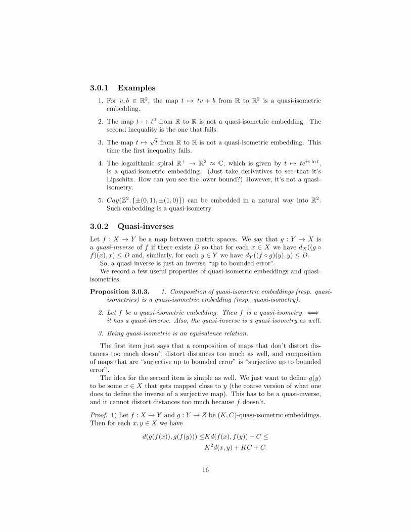
3.0.1 Examples

1. For v, b ∈ R2, the map t 7→ tv + b from R to R2 is a quasi-isometricembedding.

2. The map t 7→ t2 from R to R is not a quasi-isometric embedding. Thesecond inequality is the one that fails.

3. The map t 7→√t from R to R is not a quasi-isometric embedding. This

time the first inequality fails.

4. The logarithmic spiral R+ → R2 ≈ C, which is given by t 7→ teiπ ln t,is a quasi-isometric embedding. (Just take derivatives to see that it’sLipschitz. How can you see the lower bound?) However, it’s not a quasi-isometry.

5. Cay(Z2, {±(0, 1),±(1, 0)}) can be embedded in a natural way into R2.Such embedding is a quasi-isometry.

3.0.2 Quasi-inverses

Let f : X → Y be a map between metric spaces. We say that g : Y → X isa quasi-inverse of f if there exists D so that for each x ∈ X we have dX((g ◦f)(x), x) ≤ D and, similarly, for each y ∈ Y we have dY ((f ◦ g)(y), y) ≤ D.

So, a quasi-inverse is just an inverse “up to bounded error”.We record a few useful properties of quasi-isometric embeddings and quasi-

isometries.

Proposition 3.0.3. 1. Composition of quasi-isometric embeddings (resp. quasi-isometries) is a quasi-isometric embedding (resp. quasi-isometry).

2. Let f be a quasi-isometric embedding. Then f is a quasi-isometry ⇐⇒it has a quasi-inverse. Also, the quasi-inverse is a quasi-isometry as well.

3. Being quasi-isometric is an equivalence relation.

The first item just says that a composition of maps that don’t distort dis-tances too much doesn’t distort distances too much as well, and compositionof maps that are “surjective up to bounded error” is “surjective up to boundederror”.

The idea for the second item is simple as well. We just want to define g(y)to be some x ∈ X that gets mapped close to y (the coarse version of what onedoes to define the inverse of a surjective map). This has to be a quasi-inverse,and it cannot distort distances too much because f doesn’t.

Proof. 1) Let f : X → Y and g : Y → Z be (K,C)-quasi-isometric embeddings.Then for each x, y ∈ X we have

d(g(f(x)), g(f(y))) ≤Kd(f(x), f(y)) + C ≤K2d(x, y) +KC + C.

16

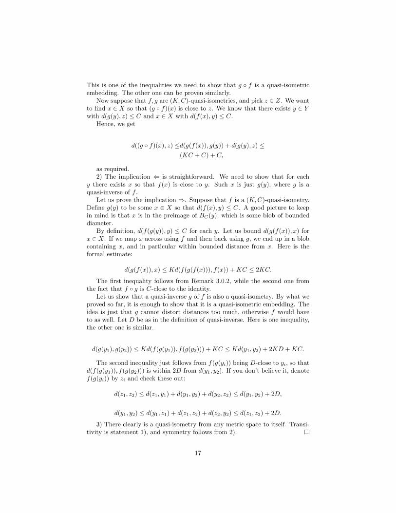
This is one of the inequalities we need to show that g ◦ f is a quasi-isometricembedding. The other one can be proven similarly.

Now suppose that f, g are (K,C)-quasi-isometries, and pick z ∈ Z. We wantto find x ∈ X so that (g ◦ f)(x) is close to z. We know that there exists y ∈ Ywith d(g(y), z) ≤ C and x ∈ X with d(f(x), y) ≤ C.

Hence, we get

d((g ◦ f)(x), z) ≤d(g(f(x)), g(y)) + d(g(y), z) ≤(KC + C) + C,

as required.2) The implication ⇐ is straightforward. We need to show that for each

y there exists x so that f(x) is close to y. Such x is just g(y), where g is aquasi-inverse of f .

Let us prove the implication ⇒. Suppose that f is a (K,C)-quasi-isometry.Define g(y) to be some x ∈ X so that d(f(x), y) ≤ C. A good picture to keepin mind is that x is in the preimage of BC(y), which is some blob of boundeddiameter.

By definition, d(f(g(y)), y) ≤ C for each y. Let us bound d(g(f(x)), x) forx ∈ X. If we map x across using f and then back using g, we end up in a blobcontaining x, and in particular within bounded distance from x. Here is theformal estimate:

d(g(f(x)), x) ≤ Kd(f(g(f(x))), f(x)) +KC ≤ 2KC.

The first inequality follows from Remark 3.0.2, while the second one fromthe fact that f ◦ g is C-close to the identity.

Let us show that a quasi-inverse g of f is also a quasi-isometry. By what weproved so far, it is enough to show that it is a quasi-isometric embedding. Theidea is just that g cannot distort distances too much, otherwise f would haveto as well. Let D be as in the definition of quasi-inverse. Here is one inequality,the other one is similar.

d(g(y1), g(y2)) ≤ Kd(f(g(y1)), f(g(y2))) +KC ≤ Kd(y1, y2) + 2KD +KC.

The second inequality just follows from f(g(yi)) being D-close to yi, so thatd(f(g(y1)), f(g(y2))) is within 2D from d(y1, y2). If you don’t believe it, denotef(g(yi)) by zi and check these out:

d(z1, z2) ≤ d(z1, y1) + d(y1, y2) + d(y2, z2) ≤ d(y1, y2) + 2D,

d(y1, y2) ≤ d(y1, z1) + d(z1, z2) + d(z2, y2) ≤ d(z1, z2) + 2D.

3) There clearly is a quasi-isometry from any metric space to itself. Transi-tivity is statement 1), and symmetry follows from 2).

17

3.0.3 Cayley graphs and quasi-isometries

And now we are ready to show that “the” Cayley graph of a given group iswell-defined up to quasi-isometry.

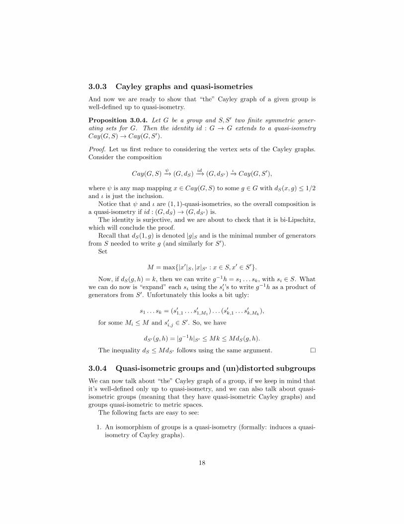
Proposition 3.0.4. Let G be a group and S, S′ two finite symmetric gener-ating sets for G. Then the identity id : G → G extends to a quasi-isometryCay(G,S)→ Cay(G,S′).

Proof. Let us first reduce to considering the vertex sets of the Cayley graphs.Consider the composition

Cay(G,S)ψ−→ (G, dS)

id−→ (G, dS′)ι−→ Cay(G,S′),

where ψ is any map mapping x ∈ Cay(G,S) to some g ∈ G with dS(x, g) ≤ 1/2and ι is just the inclusion.

Notice that ψ and ι are (1, 1)-quasi-isometries, so the overall composition isa quasi-isometry if id : (G, dS)→ (G, dS′) is.

The identity is surjective, and we are about to check that it is bi-Lipschitz,which will conclude the proof.

Recall that dS(1, g) is denoted |g|S and is the minimal number of generatorsfrom S needed to write g (and similarly for S′).

Set

M = max{|x′|S , |x|S′ : x ∈ S, x′ ∈ S′}.

Now, if dS(g, h) = k, then we can write g−1h = s1 . . . sk, with si ∈ S. Whatwe can do now is “expand” each si using the s′i’s to write g−1h as a product ofgenerators from S′. Unfortunately this looks a bit ugly:

s1 . . . sk = (s′1,1 . . . s′1,M1

) . . . (s′k,1 . . . s′k,Mk

),

for some Mi ≤M and s′i,j ∈ S′. So, we have

dS′(g, h) = |g−1h|S′ ≤Mk ≤MdS(g, h).

The inequality dS ≤MdS′ follows using the same argument.

3.0.4 Quasi-isometric groups and (un)distorted subgroups

We can now talk about “the” Cayley graph of a group, if we keep in mind thatit’s well-defined only up to quasi-isometry, and we can also talk about quasi-isometric groups (meaning that they have quasi-isometric Cayley graphs) andgroups quasi-isometric to metric spaces.

The following facts are easy to see:

1. An isomorphism of groups is a quasi-isometry (formally: induces a quasi-isometry of Cayley graphs).

18

2. If H is a subgroup of G, then the inclusion is a quasi-isometry if and onlyif H has finite index in G.

3. A surjective homomorphism G→ H is a quasi-isometry if and only if thekernel is finite.

Passing to a finite index subgroup or modding out a finite normal subgroupshould be seen as “finite perturbations” that cannot be seen from the point ofview of quasi-isometries.

Inspired by 2), one may wonder whether the inclusion of a (finitely gener-ated) subgroup in the ambient group is always a quasi-isometric embedding.Unfortunately, this is not the case. Such is life.

Subgroups whose inclusions are a quasi-isometric embeddings are calledundistorted, the other ones are called distorted. Here are some examples, thatare going to give us a good excuse to introduce a couple of interesting groups.

1. Any subgroup of an abelian group is undistorted. Exercise.

2. We will see that any cyclic subgroup of a hyperbolic group is undistorted.This is not true for all subgroups, however.

3. The subgroup generated by a in BS(1, 2) = 〈a, t|tat−1 = a2〉 is isomorphicto Z and distorted (while the one generated by t is undistorted).

4. The subgroup generated by z in the Heisenberg group 〈x, y, z|[x, y] =z, [x, z] = [y, z] = 1〉 is isomorphic to Z and distorted.

Let us elaborate a bit on item 3). Let us take for granted that a has infiniteorder. Now, it is easy to inductively see that

a2n = tnat−n.

For example, t2at−2 = t(tat−1)t−1 = ta2t−1 = tat−1tat−1 = a4.In particular, with respect to the generating set given above, d(1, a2n) ≤

2n + 1. The exponent of a and the distance are then definitely not linearlyrelated, and hence 〈a〉 is (exponentially) distorted.

By the way, BS stands for Baumslag-Solitar, and BS(1, 2) is a Baumslag-Solitar group. The groups BS(m,n) are defined as 〈a, t|tamt−1 = an〉, and theyare a good source of (counter)examples.

Let us now analyse item 3), once again taking for granted that the order ofz is infinite. Let us start from xnyn. Suppose that we want to move all y’s tothe left of the x’s. Let us start from the leftmost y. From [x, y] = z we seethat we can switch it with the rightmost x creating a z. Also, z commutes witheverything, so we can just move it to the right. Now, we can repeat and moveour y one step further to the left, once again creating a z. Repeating this, weget

xnyn = yxnyn−1zn = · · · = ynxnzn2

.

19

So, zn2

= x−ny−nxnyn, and hence d(1, zn2

) ≤ 4n. This shows that 〈z〉 is(quadratically) distorted.

Now, a few words on the Heisenberg group. Another way of describing it isas the group of the 3-by-3 upper-triangular matrices with 1’s on the diagonal: 1 Z Z

0 1 Z0 0 1

The generators written above are the following ones:

x =

1 1 01 0

1

y =

1 0 01 1

1

z =

1 0 11 0

1

Notice that the Heisenberg group is nilpotent, and actually one of the sim-

plest non-abelian nilpotent groups. Also, it is the fundamental group of a 3-manifold, constructed in the following way. Take a torus T = S1 × S1, andconsider T × [0, 1]. Now, given a homeomorphism φ : (T × {0}) → (T × {1}),one can construct the so-called mapping torus of φ by identifying T × {0} andT×{1} via φ. For a suitable choice of φ, the resulting manifold has fundamentalgroup isomorphic to the Heisenberg group. Can you describe one such φ?

3.1 The final exercise

Exercise. Suppose the the finitely generated group G is quasi-isometric to R.Then G is virtually Z.

20

Chapter 4

Milnor-Svarc Lemma

In this chapter we put together several of the concepts that we have seen so far.The following Theorem tells us that when you have a group acting nicely on ageodesic metric space, then the Cayley graph of your group looks like the spacebeing acted on. It is sometimes called the fundamental lemma of GeometricGroup Theory, and it is probably the main reason why one might wish to studygroups up to quasi-isometry.

Theorem 4.0.1. (Milnor-Svarc Lemma) Suppose that the group G acts properlyand coboundedly on the geodesic metric space X. Then

1. G is finitely generated

2. Cay(G) is quasi-isometric to X, via the map1 g 7→ gx0 for any givenchoice of x0 ∈ X.

One of the motivating examples of proper cobounded actions arises in thefollowing way. Let M be a compact, connected Riemannian manifold. Itsuniversal cover M is in a natural way also a Riemannian manifold, and π1(M)acts on it by isometries. Such action is proper and cobounded, so π1(M) is

quasi-isometric to M . In particular, one can use Milnor-Svarc Lemma to putrestrictions on the kinds of Riemannian metrics that a given manifold can carry.More on this later...

Proof. Fix x0 ∈ X, and let R be so that every x ∈ X is within distance R fromgx0 for some g ∈ G. Such R exists because the action is cobounded. Now,consider the subset of G of all elements that map x0 within distance 2R + 1from itself. In formulas:

S = {g ∈ G : d(x0, gx0) ≤ 2R+ 1}.1The map is defined only on the vertex set, so formally one should extend it. No big deal,

right?

21

Notice that S is finite because the action is proper. (S contains the identityand so it does not satisfy our standing assumptions on generating sets. We aregoing to ignore this.)

Ok, we are now ready for the core of the proof.

• S generates G. Also, |g|S ≤ dX(x0, gx0) + 2 for each g ∈ G.

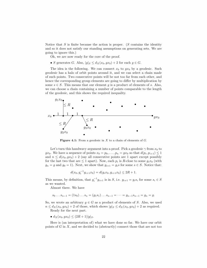
The idea is the following. We can connect x0 to gx0 by a geodesic. Suchgeodesic has a halo of orbit points around it, and we can select a chain madeof such points. Two consecutive points will be not too far from each other, andhence the corresponding group elements are going to differ by multiplication bysome s ∈ S. This means that our element g is a product of elements of s. Also,we can choose a chain containing a number of points comparable to the lengthof the geodesic, and this shows the required inequality.

Figure 4.1: From a geodesic in X to a chain of elements of G.

Let’s turn this handwavy argument into a proof. Pick a geodesic γ from x0 togx0. We have a sequence of points x0 = p0, . . . , pn = gx0 so that d(pi, pi+1) ≤ 1and n ≤ d(x0, gx0) + 2 (say all consecutive points are 1 apart except possiblyfor the last two that are ≤ 1 apart). Now, each pi is R-close to some gix0 (withgn = g and g0 = 1). Next, we show that gi+1 = gis for some s ∈ S. Notice that:

d(x0, g−1i gi+1x0) = d(gix0, gi+1x0) ≤ 2R+ 1.

This means, by definition, that g−1i gi+1 is in S, i.e. gi+1 = gisi for some si ∈ S

as we wanted.Almost there. We have

s0 . . . sn−1 = (1s0) . . . sn = (g1s1) . . . sn−1 = · · · = gn−1sn−1 = gn = g.

So, we wrote an arbitrary g ∈ G as a product of elements of S. Also, we usedn ≤ dX(x0, gx0) + 2 of those, which shows |g|S ≤ dX(x0, gx0) + 2 as required.

Ready for the next part.

• dX(x0, gx0) ≤ (2R+ 1)|g|S .

Here is (an interpretation of) what we have done so far. We have our orbitpoints of G in X, and we decided to (abstractly) connect those that are not too

22

far way from each other, and we got something connected. Now, if we have away of going from one point of G to another using the connections we created,then this “projects” to a way of connecting the corresponding orbit points inX. This is how we are going to get the required estimate.

Write g = s1 . . . sk, with k = |g|S . Denote gi = s1 . . . si (with g0 = 1).Notice that gix0 is not far from gi+1x0:

dX(gix0, gi+1x0) = dX(x0, g−1i gi+1x0) = d(x0, si+1x0) ≤ 2R+ 1.

So,

dX(x0, gx0) ≤∑

dX(gix0, gi+1x0) ≤ (2R+ 1)k = (2R+ 1)|g|S ,

as required.The bullets above (and the fact that the action on X is by isometries) easily

imply the inequalities needed to show that g 7→ gx0 is a quasi-isometric embed-ding (on the vertex set of Cay(G,S)). The image is R-dense by coboundedness,hence we really described a quasi-isometry.

4.1 A digression on growth

The material in this section is mostly independent from what is going to happennext. The aim is to introduce an interesting and simple-to-define quasi-isometryinvariant that we can couple with Milnor-Svarc Lemma to get some corollaries.

Let G be generated by the finite set S. We define βG,S(n) simply as thecardinality of the ball in (G, dS) of radius n, and we call βG,S the growth functionof G with respect to S.

Here are some examples. In each case with respect to the standard generatingsets, we have:

• βZ,S(n) = 2n+ 1,

• βZ2,S(n) = 2n2 + 2n+ 1,

• βFm,S(n) = 2m(2m− 1)n−1, where Fm is the free group on m generators,

• βH,S(n) = Θ(n4), where H is the Heisenberg group.

The last example is somehow the most surprising one. It is natural to thinkof the Heisenberg group as a 3-dimensional object, so one might expect that thegrowth function goes like n3 rather than n4. The metaphysical reason for whyit really should be of order n4 is that, while the x and y directions contribute 1to the growth exponent, the z direction contributes 2 because it is quadraticallydistorted and hence there are order of n2 elements in the z direction withindistance n of the identity. In order to prove this, you may wish to write elementsin the Heisenberg group in an appropriate normal form...

23

As usual, we are interested in groups, not pairs group/generating set. Inorder to get rid of the dependence on the generating set, we define (a partialorder and) an equivalence relation on the collection of functions.

Let f, g : N → N. Write f � g is there exists some constant C so that foreach n ∈ N we have

f(n) ≤ Cg(Cn+ C).

One way to think about it is that for n’s “at the same scale”, f(n) should be“at most of the same order of magnitude” as g(n). Further, we write f � g iff � g and g � f , while we write f ≺ g if f � g but g � f .

Here are basic examples, that after all tell you that � is not too bad, exceptmaybe that it doesn’t distinguish exponential functions.

• If 0 < a < b then na ≺ nb.

• If 1 < α < β then αn � βn.

• for each a > 0, na ≺ 2n.

So, at least we can distinguish exponents of polynomial growth, and we candistinguish polynomial functions from exponential functions.

The definition we gave is the right one to make sure that the �-class of thegrowth function does not depend on the generating set. But more is true.

Proposition 4.1.1. The �-class of the growth function is a quasi-isometryinvariant of groups.

Before proving the proposition (which is not that difficult), let us discusssome applications. The original motivation for Milnor to show the Milnor-Svarc Lemma was that he wanted to study growth functions of fundamentalgroups of Riemannian manifolds. For example, combining Milnor-Svarc Lemma,a slightly improved version of the Proposition, and well-known volume estimatesin Riemannian geometry, one (Milnor) can show that the fundamental group of acompact Riemannian manifold with negative sectional curvature has exponentialgrowth. In particular, for example, the 3-manifold whose fundamental group isthe Heisenberg group that we mentioned in Subsection 3.0.4 cannot carry such aRiemannian metric, because the growth of the Heisenberg group is polynomial.

Let us now prove the Proposition.

Proof. Let G,H be groups equipped with the finite generating sets S, T , respec-tively. Let f : G → H be a (K,C)-quasi-isometric embedding. We need twofacts that follow easily from the definition of quasi-isometric embedding.

The first one is that the image of a ball BG(1, n) of radius n in G is containedin a ball of radius Kn+ C in H.

The second one is that the preimage of any element of H contains at most,say, M elements. This is because it is entirely contained in a ball of radius,say, KC + 1 (two points further away than that cannot be mapped to the samepoint).

24

Combining the two facts we get:

#BG(1, n) ≤M ·#BH(1,Kn+ C),

one of the inequalities we wanted. The other one can be proven in the sameway using a quasi-inverse of f .

When talking about growth, it is impossible not state the following result ofGromov:

Theorem 4.1.2. A finitely generated group has at most polynomial growth ifand only if it is virtually nilpotent.

In particular, being virtually nilpotent, a purely algebraic property, is aquasi-isometry invariant.

There’s also another result that comes to mind when talking about growth.We saw examples of groups with polynomial growth, and it is easy to see that anygroup containing a free subgroup has exponential growth, so we get examplesof exponential growth as well. Is there anything in between? The answer is yes.In fact, Grigorchuck constructed groups that have growth type en

α

for some0 < α < 1.

25

Part II

Hyperbolic spaces andgroups

26

Chapter 5

Definition, examples andquasi-isometry invariance

Hyperbolic spaces are defined by a very simple property of geodesic triangles,but their theory is amazingly rich. Having a sufficiently nice action on a hyper-bolic metric space has a lot of consequences.

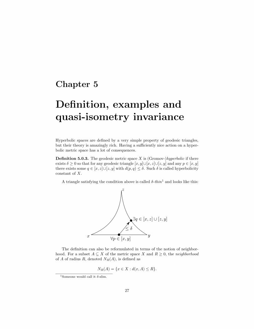
Definition 5.0.3. The geodesic metric space X is (Gromov-)hyperbolic if thereexists δ ≥ 0 so that for any geodesic triangle [x, y]∪[x, z]∪[z, y] and any p ∈ [x, y]there exists some q ∈ [x, z]∪[z, y] with d(p, q) ≤ δ. Such δ is called hyperbolicityconstant of X.

A triangle satisfying the condition above is called δ-thin1 and looks like this:

The definition can also be reformulated in terms of the notion of neighbor-hood. For a subset A ⊆ X of the metric space X and R ≥ 0, the neighborhoodof A of radius R, denoted NR(A), is defined as

NR(A) = {x ∈ X : d(x,A) ≤ R}.1Someone would call it δ-slim.

27

We can then say that X is hyperbolic if there exists δ ≥ 0 so that for anygeodesic triangle [x, y] ∪ [x, z] ∪ [z, y] we have

[x, y] ⊆ Nδ([x, z] ∪ [z, y]).

We will show that being hyperbolic is a quasi-isometry invariant of geodesicmetric spaces. Accepting this for the moment, we can define what it means fora group to be hyperbolic.

Definition 5.0.4. The finitely generated group G is hyperbolic if one of thefollowing equivalent conditions hold.

1. G has one hyperbolic Cayley graph.

2. Every Cayley graph of G is hyperbolic.

3. G acts properly and coboundedly on a hyperbolic metric space.

The third condition is equivalent to the other two by Milnor-Svarc Lemmaand quasi-isometry invariance of hyperbolicity.

5.1 Examples (for the moment!)

Let us start from the uninteresting examples.

• Metric spaces of bounded diameter are hyperbolic, just take the diameteras δ.

• R is hyperbolic, as every triangle is degenerate.

And now let us move on to more interesting examples.

• Free groups are hyperbolic. Remember that a free group (on at least twogenerators) has a Cayley graph that looks like this:

For such Cayley graph, we can actually take δ = 0, i.e. any side of ageodesic triangle is contained in the union of the other two sides, like inthis picture:

28

• The hyperbolic plane H2 is hyperbolic (this is where the name comesfrom), and the same is true for the higher dimensional hyperbolic spacesHn. Recall that for g ≥ 2, the connected compact boundary-less surfaceSg of genus g admits a Riemannian metric whose universal cover is H2.In particular, π1(Sg) is hyperbolic.

• More in general, for a compact Riemannian manifold M , we have thatπ1(M) is hyperbolic if and only if M is. (Almost) concrete examples ofsuch manifolds in dimension 3 can be constructed as follows. For g ≥ 2,consider Sg × [0, 1], which has two boundary components homeomorphicto Sg. If we give a homeomorphism of Sg, we can use it to glue the twoboundary component and obtain a 3-manifold without boundary. As itturns out, due to a theorem of Thurston, if we choose the gluing map to bea “pseudo-Anosov” (whatever that means), then the manifold M we gethas a Riemannian metric with universal cover H3, so that its fundamentalgroup is hyperbolic. In algebraic terms, the fundamental group can bedescribed by a short exact sequence of the type

1→ π1(Sg)→ π1(M)→ Z→ 1.

We will see more (algebraic/combinatorial) examples later...

5.2 Non-examples

• R2 and Z2 are not hyperbolic. This is easy.

• More in general, any group containing a copy of Z2 is not hyperbolic.We’ll see this.

• BS(1, 2) and the Heisenberg group are not hyperbolic, for example becausethey contain distorted cyclic subgroups, while we will see that this cannotbe the case for hyperbolic groups. (The Heisenberg group also containsZ2.)

29

5.3 List of properties

The point of this section is to impress you with the amount of stuff that isknown about hyperbolic spaces. We will see proofs of several of these facts.

• Hyperbolic groups are finitely presented, i.e. every hyperbolic group hasa presentation with finitely many (generators and) relators.

• When given a finite presentation, you can ask yourself how you can de-termine whether a given word in the generating set represents the trivialelement or not. This, a bit surprisingly, is not doable in general. In someother cases, there exist only very slow algorithms to do that. However,for any given presentation of a hyperbolic group there is a linear timealgorithm to determine whether a given word represents the identity ornot.

• Any hyperbolic group has finitely many conjugacy classes of finite sub-groups.

• The centraliser of any infinite order element of a hyperbolic group is vir-tually Z, i.e. almost as small as possible.

• Cyclic subgroups of hyperbolic groups are undistorted.

There are also some “largeness” properties that only require a very mildadditional condition. If the group G is hyperbolic and not virtually cyclic(in particular, not finite), then:

• G contains a copy of the free group F2 on two generators. In particular,G has exponential growth (i.e., it grows as fast as possible).

• G is SQ-universal, i.e. any countable group embeds in some quotient of G.In particular, G has uncountably many non-isomorphic quotients, becausethere are uncountably many non-isomorphic finitely generated groups andany given finitely generated group contains only countably many finitelygenerated subgroups.

5.4 Quasi-isometry invariance

In this section we show the quasi-isometry invariance of hyperbolicity. Thenotion of hyperbolicity is stated in terms of geodesics, but the image of a geodesicvia a quasi-isometry need not be a geodesic. However, we will show that in asuitable sense it is within bounded distance from a geodesic, if the ambient spaceis hyperbolic.

Definition 5.4.1. A (K,C)-quasi-geodesic in the metric space X is a (K,C)-quasi-isometric embedding of some interval in R into X.

30

The reason why we gave this definition is because the image of a geodesic γvia a (K,C)-quasi-isometric embedding is a (K,C)-quasi-geodesic2

It is convenient to introduce now the notion of Hausdorff distance, which isa sensible way of measuring how different two subsets of a metric space are.

Let A,B be subsets of a given metric space, then their Hausdorff distance isdefined as

dHaus(A,B) = inf{R : A ⊆ NR(B), B ⊆ NR(A)}.

A good way to think about it is: If every point in A is within distanceR from B and viceversa, then we have dHaus(A,B) ≤ R. And conversely,if dHaus(A,B) ≤ R then every point in A is within distance R from B andviceversa.

The informal version of the following statement is that quasi-geodesics inhyperbolic spaces stay close to geodesics.

Proposition 5.4.2. Let X be hyperbolic. Then for every K,C there exists D sothat for any quasi-geodesic ρ and any geodesic γ = [x, y] with the same endpointsx, y as ρ, we have that the Hausdorff distance between (the images of) γ and ρis at most D.

The analogous statement for R2 is false. For examples, following the x-axis for a while and then the y-axis gives quasi-geodesics (with uniform con-stants) that cannot possibly be within uniformly bounded Hausdorff distancefrom geodesics. Another counterexample is given by the logarithmic spiral thatwas mentioned among the examples of quasi-isometric embeddings.

And here is the corollary we were aiming for.

Corollary 5.4.3. Let X,Y be geodesic metric spaces. If there exists a quasi-isometric embedding f : X → Y and Y is hyperbolic, then so is X.

In particular, if the geodesic metric spaces X,Y are quasi-isometric, then Xis hyperbolic if and only if Y is hyperbolic.

In order to prove the corollary we just need to push forward geodesic trianglesin X to quasi-geodesic triangles in Y , use that quasi-geodesic triangles in Y arethin and deduce that triangles in X are thin because f doesn’t distort distancestoo much.

Proof. Let’s give name to the constants. Let δ be a hyperbolicity constant forY and suppose that f : X → Y is a (K,C)-quasi-isometric embedding and letD be as in Proposition 5.4.2.

Ok, now consider a geodesic triangle [x, y] ∪ [x, z] ∪ [z, y] in X and p ∈[x, y]. Then f(p) is D-close to some p1 on a geodesic from f(x) to f(y). Byhyperbolicity and up to switching x and y, p1 is δ-close to some p2 on a geodesic

2This is slightly imprecise. What is true is that the image of a geodesic parametrisedby arc length is a quasi-geodesic, where a geodesic parametrised by arc length is a mapγ : (I ⊆ R) → X so that d(γ(t1), γ(t2)) = |t1 − t2| for every ti ∈ I. Any geodesic can bereparametrised to have this property.

31

from f(x) to f(z). Finally, p2 is D-close to f(q) for some q ∈ [x, z]. So, weonly need to show that p and q are close. This is easy: We have d(f(p), f(q)) ≤2D + δ, and so, using that f is a (K,C)-quasi-isometric embedding we getd(p, q) ≤ (2D + δ)K +KC.

5.4.1 Proof of Proposition 5.4.2

We will use the following preliminary lemma that basically says that we canreplace any quasi-geodesic with a “tamer” one that stays in in a controlledneighborhood of the first one.

Lemma 5.4.4. For any K,C there exist K ′, C ′, D so that the following holds.For any (K,C)-quasi-geodesic γ to a geodesic metric space X there exists a(K ′, C ′)-quasi-geodesic γ′ so that:

1. γ′ has the same endpoints as γ,

2. dHaus(γ, γ′) ≤ D.

3. for any subpath β of γ, say from a to b, we have l(β) ≤ K ′d(a, b) + C ′.

The proof is remarkably tedious and not very interesting, so we will skip it.A detailed argument is presented in [Bridson-Haefliger]. The idea is easy: if thedomain of γ is I, you look at γ(I ∩ Z) and interpolate with geodesics.

Notation. Unless otherwise stated, from now on we fix the notation ofProposition 5.4.2, and δ will denote a hyperbolicity constant for X. Further-more, we assume that the quasi-geodesic ρ satisfies the conditions of the lemma(with K,C replacing K ′, C ′). In view of the lemma, it is enough to prove theproposition for such quasi-geodesics. We will also assume d(x, y) ≥ 1.

The proof can be split in three parts.

The logarithmic estimate

For the moment, we show that the distance from any point on the geodesic tothe quasi-geodesic is bounded logarithmically in the length of the quasi-geodesic.The content of this part of the proof is the following lemma.

Lemma 5.4.5. Let X be a hyperbolic space with hyperbolicity constant δ. Sup-pose that p ∈ X lies on the geodesic [x, y] and that α is a path from x to y, oflength at least 1. Then

d(p, α) ≤ δ log2(l(α)) + 2.

Proof. We can assume that the length of α is finite.If l(α) ≤ 2, then the statement is clear because d(x, y) ≤ 2 and hence

d(p, α) ≤ d(p, x) ≤ 2.The core of the proof consists in splitting α into two parts of equal length

and proceeding inductively, the base case being l(α) ≤ 2.

32

Suppose l(α) ≥ 2. Let q ∈ α be so that q splits α into two parts α1, α2 ofequal length. We know that p is within distance δ from some point p′ eitheron a geodesic [x, q] or a geodesic [q, y], let us say that the first case holds andthat α1 is the part of α with endpoints x, q. So, using induction we have thestraightforward computation:

d(p, α) ≤ d(p, p′) + d(p′, α1) ≤

δ + δ log2

(l(α)/2

)+ 2 = δ log2(l(α)) + 2.

That’s it.

As the length of the quasi-geodesic ρ is at most Kd(x, y) + C we get thefollowing.

Corollary 5.4.6. In the notation of Proposition 5.4.2, for any p ∈ [x, y] wehave d(p, ρ) ≤ δ log2(Kd(x, y) + C) + 2.

Picking the worst point

In this subsection we show that for each p ∈ [x, y] we have d(p, ρ) ≤ m, for somem that depends on K,C, δ only.

The strategy we adopt now to improve the logarithmic estimate is pickingthe “worst point” along [x, y], meaning the one furthest away from the quasi-geodesic ρ, and try to find some configuration that allows us to jump efficientlyfrom p to ρ.

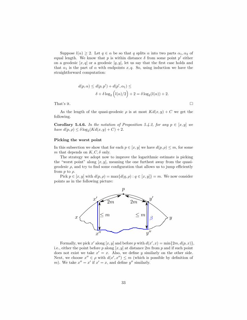
Pick p ∈ [x, y] with d(p, ρ) = max{d(q, ρ) : q ∈ [x, y]} = m. We now considerpoints as in the following picture:

Formally, we pick x′ along [x, y] and before p with d(x′, x) = min{2m, d(p, x)},i.e., either the point before p along [x, y] at distance 2m from p and if such pointdoes not exist we take x′ = x. Also, we define y similarly on the other side.Next, we choose x′′ ∈ ρ with d(x′, x′′) ≤ m (which is possible by definition ofm). We take x′′ = x′ if x′ = x, and define y′′ similarly.

33

The reason why we moved a distance 2m from p is that any point on ageodesic [x′, x′′] or [y′, y′′] has distance at least 2m−m = m from p. So, if β isthe concatenation of [x′, x′′], a subpath of ρ from x′′ to y′′ and [y′′, y′], we have• d(p, β) ≥ m.Also, d(x′′, y′′) ≤ m + 2m + 2m + m = 6m. So, the length of the bottom

part of β (meaning the subpath of ρ) is at most 6mK + C, and• l(β) ≤ (6K + 2)m+ C.Putting together the logarithmic estimates and the two properties of β we

get:

m ≤d(p, β) ≤δ log2(l(β)) + 2 ≤

δ log2

((6K + 2)m+ C

)+ 2

The last term is logarithmic in m, so there is a bound on m that dependson δ,K,C only.

No large detours

We already showed half of what we wanted to prove, namely that any point on[x, y] is close to ρ. We now conclude the proof by showing that any point on ρis D-close to [x, y], for a suitable D that depends on K,C, δ.

The idea is to bound the length of the subpaths of ρ that make a “detour”outside the neighborhood Nm([x, y]), where m is as in the second part of theproof (and it depends on δ,K,C only).

Pick any q ∈ ρ. If d(q, [x, y]) ≤ m, we are happy. Otherwise, consider thetwo subpaths ρ1, ρ2 of ρ that concatenate at q. By the property of m, any pointin [x, y] is m-close to either ρ1 or ρ2. One endpoint x of [x, y] is close to ρ1,while the other one y is close to ρ2. Travelling along [x, y] we then see that atsome point p we switch from being close to ρ1 to being close to ρ2, and henced(p, qi) ≤ m for some points q1 ∈ ρ1 and q2 ∈ ρ2. The length of the subpathof ρ from q1 to q2 (which contains q!) is bounded by 2mK + C, because itsendpoints are within distance 2m of each other. In particular

d(q, [x, y]) ≤ d(q, q1) + d(q1, p) ≤ 2mK + C +m.

As q was any point on ρ, we are done.

34

Chapter 6

Hn

The aim of the chapter is to describe THE motivating examples of (Gromov-)hyperbolic spaces. Annoyingly, they are called (real) hyperbolic spaces, andthey are denoted by Hn, where n ≥ 2 is an integer.

Some Riemannian geometry is about to show up, but no worries, it will goaway soon.

6.1 Two models

One of the possible ways of defining Hn is “the unique (up to isometry) completesimply connected Riemannian manifold with all sectional curvatures −1 at everypoint”.

Luckily, there are concrete models for Hn, and actually there are several ofthem. This turns out to be very convenient because different properties of Hnare clear in different models. We now present two of the models.

The half-space model. Consider an open half-space in Rn, i.e. Rn−1 ×R>0, where we denote the first n − 1 coordinates by xi and the last one by y.The Riemannian metric on the half space that makes it (isometric to) Hn is

1

y2

(∑dx2

i + dy2).

It is important to note that the metric is a pointwise rescaling of the Euclideanmetric (i.e. the two metrics are conformally equivalent) and that it is invariantunder translations in the xi coordinates.

The ball model. Consider now the open unit ball in Rn, and denote thecoordinates by xi. We denote the square of the Euclidean norm of a pointx = (xi) by |x|2 =

∑x2i . The Riemannian metric at the point x is in this case

4

(1− |x|2)2

∑dx2

i .

Once again, the metric is a pointwise rescaling of the Euclidean metric, and inthis case it is invariant under rotations around the origin.

35

It can be seen directly that the two models are isometric. The isometrycan be described in terms of what goes under the name of inversion across acircle. We won’t describe it here, but one good thing about it is the remarkableproperty that it maps (Euclidean) lines and circles in one model to (Euclidean)lines and circles in the other one.

For concreteness, we henceforth focus on H2, the hyperbolic plane, but sev-eral of the things we are about to say hold in higher dimension as well. In thiscase, the first model is called half-plane model and the second model is calledthe disk model or Poincare disk model. We use coordinates x, y so that theRiemannian metrics of the two models become:

1

y2

(dx2 + dy2

),

and

4

(1− |x|2)2

(dx2 + dy2

),

respectively.

6.2 Lots of isometries!

One of the coolest as well as most important properties of H2 is that it is verysymmetric, meaning that it has lots of isometries. Let us describe the isometriesthat are easy to see in the two models.

6.2.1 In the half-plane model

The following transformations of the half-plane are isometries of H2. The firsttwo are clear from the formula for the Riemannian metric.

• Translations in the x coordinate, i.e. maps of the type (x, y) 7→ (x+ t, y),for some fixed t.

• Reflections across the y-axis, i.e. (x, y) 7→ (−x, y).

• Dilations, i.e. maps of type (x, y) 7→ (λx, λy) for some λ > 0.

In order to see that dilations are isometries one can just make a computation,and what one gets is that the derivative of the dilation contributes a factorλ2 to the Riemannian metric, while the 1/y2 factor contributes a factor 1/λ2.More pictorially, if one has a tiny tiny path in the half-plane, its length in thehyperbolic metric is going to be pretty much the Euclidean length times 1/y0,where y0 is the y-coordinate of the path. When hitting the half-plane with thedilation, we multiply the Euclidean length by λ, but we end up somewhere withy-coordinate λy0, so we need to rescale the new length by λy0 instead of y0. So,the two effects cancel out, which means that the dilation preserves lengths ofpaths computed in the hyperbolic metric and hence the hyperbolic metric itself.

36

Notice that we already have enough isometries to show that H2 is homo-geneous, i.e. that for any p, q ∈ H2 there is an isometry f : H2 → H2 withf(p) = q. (How can one show this?)

6.2.2 In the disk model

The following transformations of the disk are (clearly) isometries of H2.

• Reflections across diameters.

• Rotations around the origin.

Using these additional isometries one can show thatH2 is actually bi-homogeneous,meaning that for any p1, p2, q1, q2 with d(p1, p2) = d(q1, q2) there is an isometryf : H2 → H2 with f(pi) = qi.

6.3 Geodesics and hyperbolicity

As it turns out, one can describe all geodesics in H2, in both models.In the half-plane model any geodesic is either a vertical segment or it is an

arc contained in a half-circle orthogonal to the line {y = 0}.In the disk model geodesics are either segments contained in diameters or

arcs contained in circles orthogonal to the boundary:

37

One can prove these facts without using any Riemannian geometry. Instead,one can just observe that the set of all geodesics has to be invariant under allisometries of H2. We will not spell this out here, as it also requires to know ait how the isometry from one model to the other one works, but I promise it’selementary.

6.3.1 Hyperbolicity

Once one has an explicit description of the geodesics, showing that H2 is hyper-bolic becomes a reasonable task.

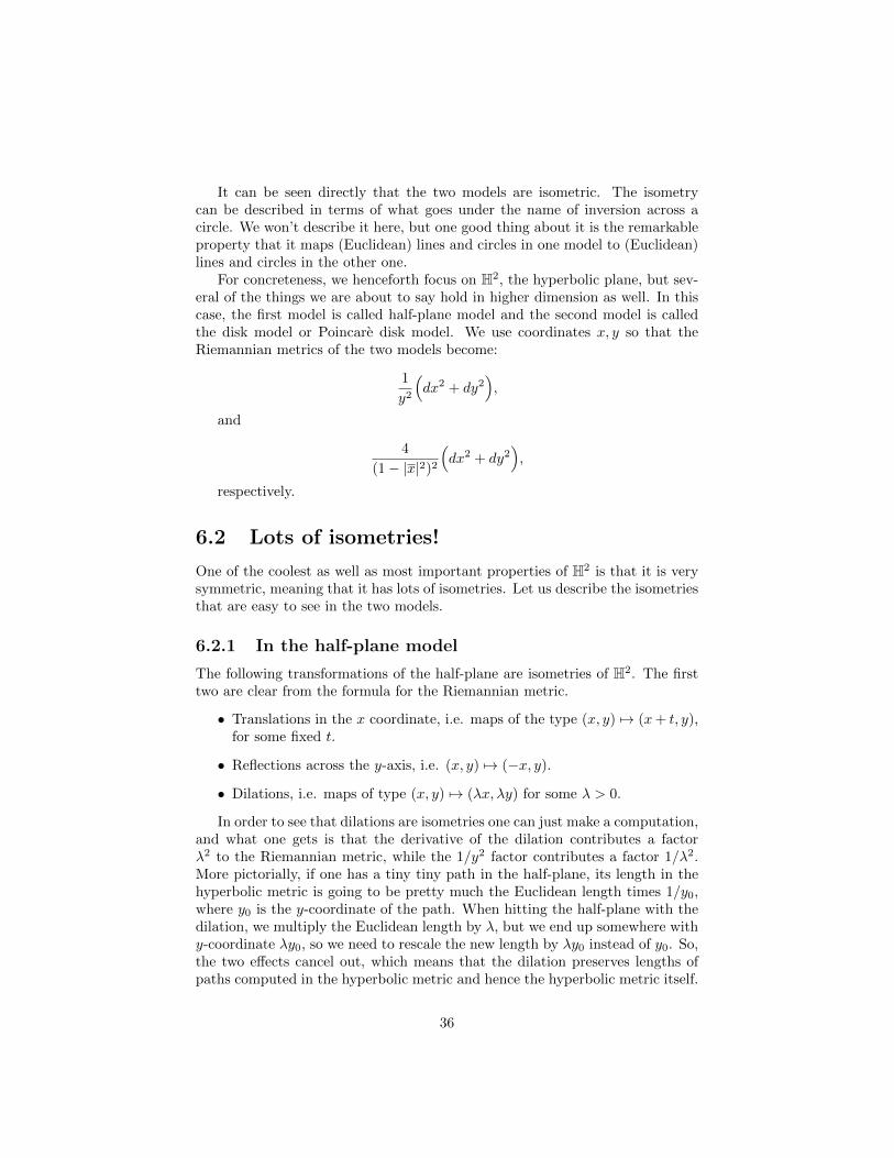
As a warm-up, one can consider an ideal triangle, that is to say the union, inthe half-plane model, of two vertical lines and a half-circle orthogonal to {y = 0}that looks like this:

We wish to show that any ideal triangle (there is actually only one up toisometry) satisfies the thinness condition. In order to do so, we ask ourselveshow a neighborhood of one of the vertical geodesics looks like. And the answeris that it has the conical shape as in the picture. The reason is that it has tobe invariant under the dilations centered at the “bottom point” of the verticalline. Increasing the angle one increases the radius of the neighborhood, and itis not hard to conclude from here finding neighborhoods as in the picture.

In order to deduce thinness of triangles in H2 from that of the ideal tri-angle(s), one can argue that a non-ideal triangle can be mapped isometricallyinside an ideal triangle.

6.4 Right-angled n-gons and hyperbolic surfaces

Here is a funny fact about H2.

38

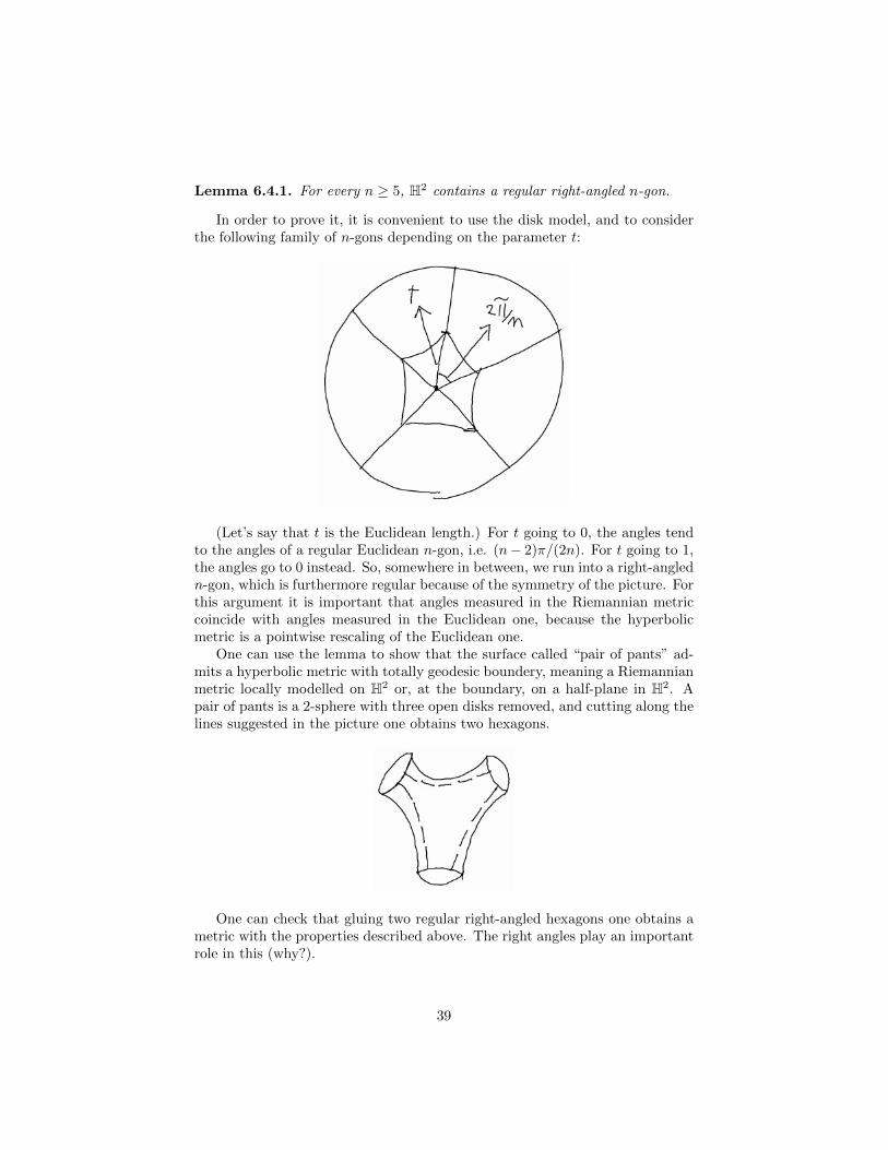
Lemma 6.4.1. For every n ≥ 5, H2 contains a regular right-angled n-gon.

In order to prove it, it is convenient to use the disk model, and to considerthe following family of n-gons depending on the parameter t:

(Let’s say that t is the Euclidean length.) For t going to 0, the angles tendto the angles of a regular Euclidean n-gon, i.e. (n− 2)π/(2n). For t going to 1,the angles go to 0 instead. So, somewhere in between, we run into a right-angledn-gon, which is furthermore regular because of the symmetry of the picture. Forthis argument it is important that angles measured in the Riemannian metriccoincide with angles measured in the Euclidean one, because the hyperbolicmetric is a pointwise rescaling of the Euclidean one.

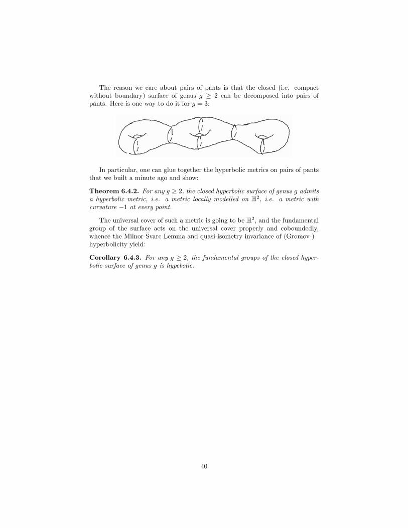
One can use the lemma to show that the surface called “pair of pants” ad-mits a hyperbolic metric with totally geodesic boundery, meaning a Riemannianmetric locally modelled on H2 or, at the boundary, on a half-plane in H2. Apair of pants is a 2-sphere with three open disks removed, and cutting along thelines suggested in the picture one obtains two hexagons.

One can check that gluing two regular right-angled hexagons one obtains ametric with the properties described above. The right angles play an importantrole in this (why?).

39

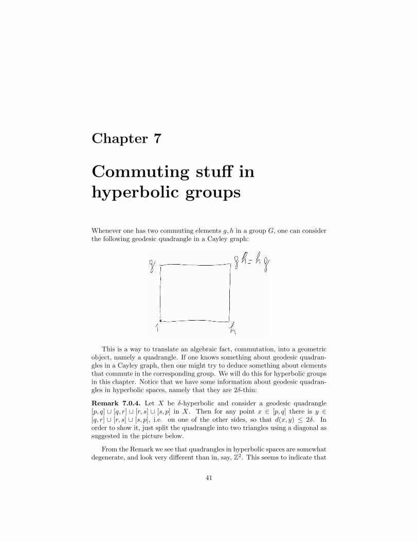
The reason we care about pairs of pants is that the closed (i.e. compactwithout boundary) surface of genus g ≥ 2 can be decomposed into pairs ofpants. Here is one way to do it for g = 3:

In particular, one can glue together the hyperbolic metrics on pairs of pantsthat we built a minute ago and show:

Theorem 6.4.2. For any g ≥ 2, the closed hyperbolic surface of genus g admitsa hyperbolic metric, i.e. a metric locally modelled on H2, i.e. a metric withcurvature −1 at every point.

The universal cover of such a metric is going to be H2, and the fundamentalgroup of the surface acts on the universal cover properly and coboundedly,whence the Milnor-Svarc Lemma and quasi-isometry invariance of (Gromov-)hyperbolicity yield:

Corollary 6.4.3. For any g ≥ 2, the fundamental groups of the closed hyper-bolic surface of genus g is hypebolic.

40

Chapter 7

Commuting stuff inhyperbolic groups

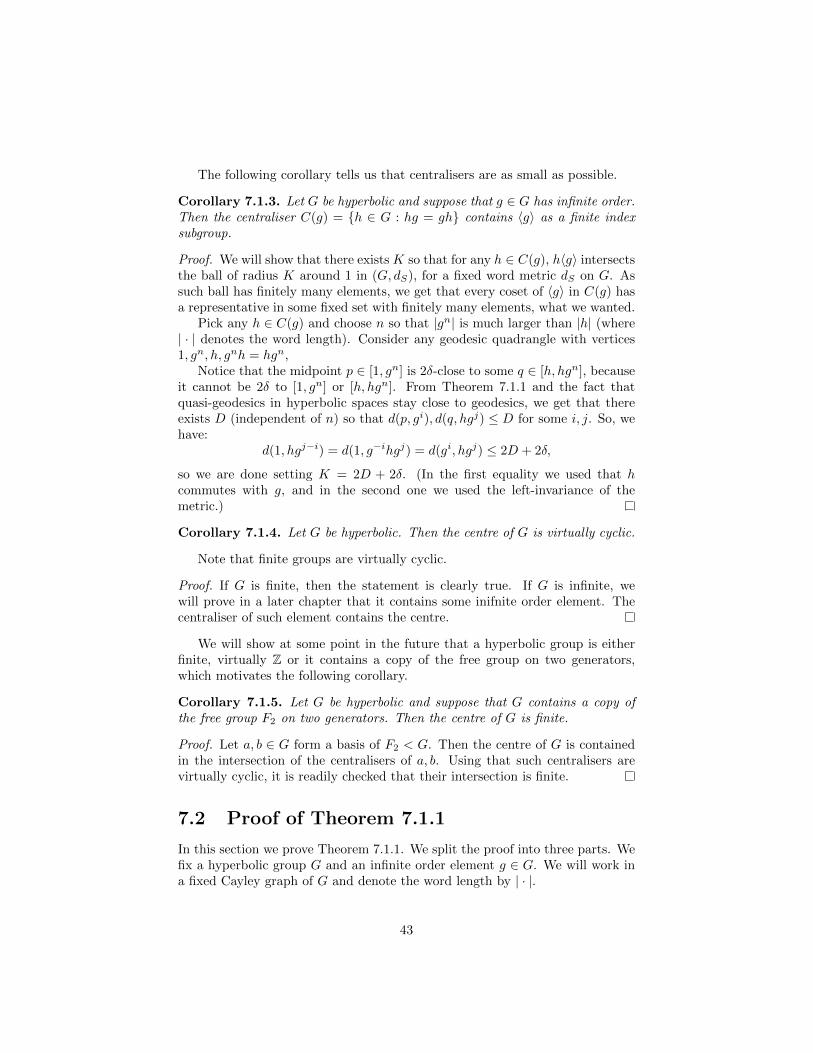
Whenever one has two commuting elements g, h in a group G, one can considerthe following geodesic quadrangle in a Cayley graph:

This is a way to translate an algebraic fact, commutation, into a geometricobject, namely a quadrangle. If one knows something about geodesic quadran-gles in a Cayley graph, then one might try to deduce something about elementsthat commute in the corresponding group. We will do this for hyperbolic groupsin this chapter. Notice that we have some information about geodesic quadran-gles in hyperbolic spaces, namely that they are 2δ-thin:

Remark 7.0.4. Let X be δ-hyperbolic and consider a geodesic quadrangle[p, q] ∪ [q, r] ∪ [r, s] ∪ [s, p] in X. Then for any point x ∈ [p, q] there is y ∈[q, r] ∪ [r, s] ∪ [s, p], i.e. on one of the other sides, so that d(x, y) ≤ 2δ. Inorder to show it, just split the quadrangle into two triangles using a diagonal assuggested in the picture below.

From the Remark we see that quadrangles in hyperbolic spaces are somewhatdegenerate, and look very different than in, say, Z2. This seems to indicate that

41

it is very rare for elements in a hyperbolic group to commute. We will see thatthis is actually the case.

7.1 Results

We start with a Theorem that will be proven in the next section. It does notinvolve commuting elements, but we will see that it has several corollaries thatdo.

Theorem 7.1.1. Let G be a hyperbolic group and suppose that g ∈ G hasinfinite order. Then 〈g〉 is undistorted in G. Equivalently, the map

Z→ G

n 7→ gn

is a quasi-isometric embedding with respect to any given word metric d on G.

Notice that we always have d(1, gn) ≤ |n|d(1, g) (if g can be written as aproduct of k generators then gn can be written as a product of |n|k generators),so that the content of the Theorem is that there is a lower bound on d(1, gn)which is linear in n. Oh, and we only need to worry about d(1, gn) and notmore general d(gm, gn) because d(gm, gn) = d(1, gn−m).

Corollary 7.1.2. Let G be hyperbolic and suppose that g ∈ G has infinite order.Then if gn is conjugate to gm, we have either m = n or m = −n.

Proof. If there was some h so that gn = hgmh−1, say with |n| > |m|, then foreach positive integer k we would have:

gnk

= hgmk

h−1.

But then we would also have, for some constants K,C not depending on k:

|n|k

K− C ≤

∣∣∣gnk ∣∣∣S≤ 2|h|S +

∣∣∣gmk ∣∣∣S≤ 2|h|S +K|m|k + C,

where S is a finite generating set for G and | · |S denotes the word length (or,equivalently, the distance from 1 in Cay(G,S)). This is impossible for k largeenough, the term on the left diverges faster than the one on the right.

42

The following corollary tells us that centralisers are as small as possible.

Corollary 7.1.3. Let G be hyperbolic and suppose that g ∈ G has infinite order.Then the centraliser C(g) = {h ∈ G : hg = gh} contains 〈g〉 as a finite indexsubgroup.

Proof. We will show that there exists K so that for any h ∈ C(g), h〈g〉 intersectsthe ball of radius K around 1 in (G, dS), for a fixed word metric dS on G. Assuch ball has finitely many elements, we get that every coset of 〈g〉 in C(g) hasa representative in some fixed set with finitely many elements, what we wanted.

Pick any h ∈ C(g) and choose n so that |gn| is much larger than |h| (where| · | denotes the word length). Consider any geodesic quadrangle with vertices1, gn, h, gnh = hgn,

Notice that the midpoint p ∈ [1, gn] is 2δ-close to some q ∈ [h, hgn], becauseit cannot be 2δ to [1, gn] or [h, hgn]. From Theorem 7.1.1 and the fact thatquasi-geodesics in hyperbolic spaces stay close to geodesics, we get that thereexists D (independent of n) so that d(p, gi), d(q, hgj) ≤ D for some i, j. So, wehave:

d(1, hgj−i) = d(1, g−ihgj) = d(gi, hgj) ≤ 2D + 2δ,

so we are done setting K = 2D + 2δ. (In the first equality we used that hcommutes with g, and in the second one we used the left-invariance of themetric.)

Corollary 7.1.4. Let G be hyperbolic. Then the centre of G is virtually cyclic.

Note that finite groups are virtually cyclic.

Proof. If G is finite, then the statement is clearly true. If G is infinite, wewill prove in a later chapter that it contains some inifnite order element. Thecentraliser of such element contains the centre.

We will show at some point in the future that a hyperbolic group is eitherfinite, virtually Z or it contains a copy of the free group on two generators,which motivates the following corollary.

Corollary 7.1.5. Let G be hyperbolic and suppose that G contains a copy ofthe free group F2 on two generators. Then the centre of G is finite.

Proof. Let a, b ∈ G form a basis of F2 < G. Then the centre of G is containedin the intersection of the centralisers of a, b. Using that such centralisers arevirtually cyclic, it is readily checked that their intersection is finite.

7.2 Proof of Theorem 7.1.1

In this section we prove Theorem 7.1.1. We split the proof into three parts. Wefix a hyperbolic group G and an infinite order element g ∈ G. We will work ina fixed Cayley graph of G and denote the word length by | · |.

43

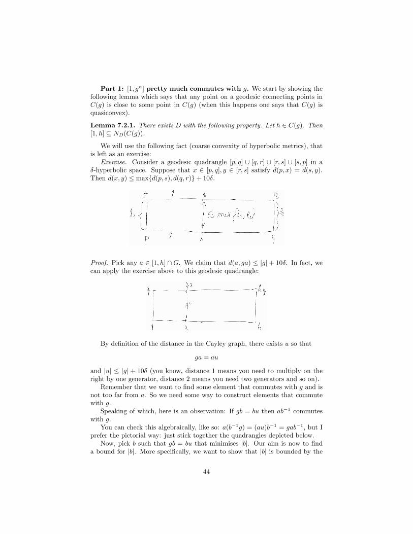
Part 1: [1, gn] pretty much commutes with g. We start by showing thefollowing lemma which says that any point on a geodesic connecting points inC(g) is close to some point in C(g) (when this happens one says that C(g) isquasiconvex).

Lemma 7.2.1. There exists D with the following property. Let h ∈ C(g). Then[1, h] ⊆ ND(C(g)).

We will use the following fact (coarse convexity of hyperbolic metrics), thatis left as an exercise:

Exercise. Consider a geodesic quadrangle [p, q] ∪ [q, r] ∪ [r, s] ∪ [s, p] in aδ-hyperbolic space. Suppose that x ∈ [p, q], y ∈ [r, s] satisfy d(p, x) = d(s, y).Then d(x, y) ≤ max{d(p, s), d(q, r)}+ 10δ.

Proof. Pick any a ∈ [1, h] ∩G. We claim that d(a, ga) ≤ |g| + 10δ. In fact, wecan apply the exercise above to this geodesic quadrangle:

By definition of the distance in the Cayley graph, there exists u so that

ga = au

and |u| ≤ |g| + 10δ (you know, distance 1 means you need to multiply on theright by one generator, distance 2 means you need two generators and so on).

Remember that we want to find some element that commutes with g and isnot too far from a. So we need some way to construct elements that commutewith g.

Speaking of which, here is an observation: If gb = bu then ab−1 commuteswith g.

You can check this algebraically, like so: a(b−1g) = (au)b−1 = gab−1, but Iprefer the pictorial way: just stick together the quadrangles depicted below.

Now, pick b such that gb = bu that minimises |b|. Our aim is now to finda bound for |b|. More specifically, we want to show that |b| is bounded by the

44

cardinality K of the ball of radius |g| + 10δ in G, which is some finite integer.In fact, for every b0 ∈ [1, b] ∩ G there exists v in such ball so that gb0 = b0v,again due to the exercise above. So, if |b| was larger than K, there would bedistinct b1, b2 ∈ [1, b] and the same v in the ball so that

gbi = biv,

for i = 1, 2. Assuming that b1 is closer to 1 than b2, it’s not hard to check that:

• b′ = b1(b−12 b) satisfies gb′ = b′u, and

• |b′| < |b|.

Doing it algebraically is a bit tedious, so we justify this pictorially: Just sticktogether the first and third quadrangle in the picture below.

Part 2: |g2n| ≈ 2|gn|.

Lemma 7.2.2. There exists C with the followng property. For every n ≥ 0, wehave d(gn, [1, g2n]) ≤ L.

Proof. Set C = 100D + 100δ + 1, for D as in Lemma 7.2.1. Suppose by con-tradiction that d(gn, [1, g2n]) > C + δ. Pick p ∈ gn[1, gn] so that d(p, gn) = C.Notice that p cannot be δ-close to [1, g2n], hence it is δ-close to some q ∈ [1, gn].By Lemma 7.2.1, there are a, b ∈ C(g) satisfying d(p, gna), d(q, gnb−1) ≤ D.

In particular,

45

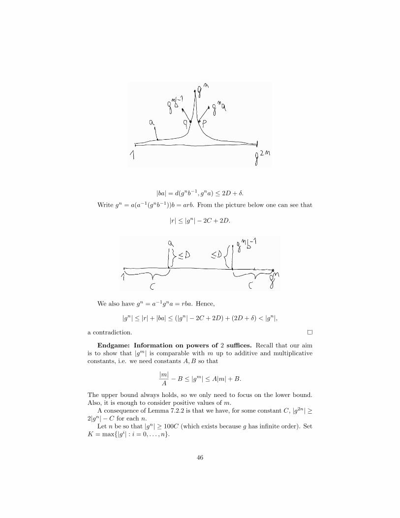
|ba| = d(gnb−1, gna) ≤ 2D + δ.

Write gn = a(a−1(gnb−1))b = arb. From the picture below one can see that

|r| ≤ |gn| − 2C + 2D.

We also have gn = a−1gna = rba. Hence,

|gn| ≤ |r|+ |ba| ≤ (|gn| − 2C + 2D) + (2D + δ) < |gn|,

a contradiction.

Endgame: Information on powers of 2 suffices. Recall that our aimis to show that |gm| is comparable with m up to additive and multiplicativeconstants, i.e. we need constants A,B so that

|m|A−B ≤ |gm| ≤ A|m|+B.

The upper bound always holds, so we only need to focus on the lower bound.Also, it is enough to consider positive values of m.

A consequence of Lemma 7.2.2 is that we have, for some constant C, |g2n| ≥2|gn| − C for each n.

Let n be so that |gn| ≥ 100C (which exists because g has infinite order). SetK = max{|gi| : i = 0, . . . , n}.

46

All we are about to do now is estimating |gm| by writing m as a sum ofterms of the form 2kn and a remainder term, and it turns out that we can getthe estimate we need in this way.

Suppose m =∑

(2kin) + r, with k1 > k2 > · · · ≥ 0 and 0 ≤ r ≤ n. Ifk2 < k1 − 1 then we have∑

i>1

2ki ≤∑

j<k1−1

2j ≤ 2k1−1

and the estimate is direct:

|gm| ≥ 2k1 |gn| − k1C −∑i>1

2i|gn| −K ≥

2k1−1|gn| − k1C −K ≥|gn|10n

m−K.

The last inequality comes from 2k1−1 ≥ m/(4n) and |gn| being much largerthan C.

If k2 = k1 − 1, then we re-write m = 2k1+1n − 2k2n +∑i≥3(2kin) + r, and

proceed similarly.

47

Chapter 8

Geometry of presentations

The main idea we will exploit in this chapter is that whenever you have agroup G generated by the symmetric set S and a word w in the alphabet Sthat represents the identity in G, then w gives a loop in Cay(G,S). Actuallythere’s a 1 − 1 correspondence between such words and combinatorial loops inCay(G,S).

Notice that in the previous chapter we exploited the special case of thisprinciple when the word represents the commutator [g, h] of two commutingelements g, h.

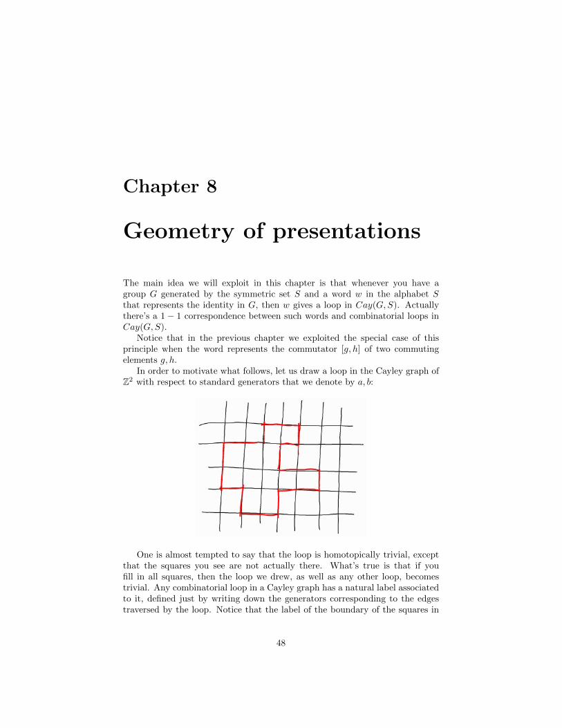
In order to motivate what follows, let us draw a loop in the Cayley graph ofZ2 with respect to standard generators that we denote by a, b:

One is almost tempted to say that the loop is homotopically trivial, exceptthat the squares you see are not actually there. What’s true is that if youfill in all squares, then the loop we drew, as well as any other loop, becomestrivial. Any combinatorial loop in a Cayley graph has a natural label associatedto it, defined just by writing down the generators corresponding to the edgestraversed by the loop. Notice that the label of the boundary of the squares in

48

the picture above is (a cyclic permutation of) [a, b] = aba−1b−1. Oh, wait, butZ2 = 〈a, b|[a, b]〉...

Let us try to generalise.

Definition 8.0.3. Let 〈S|R〉 be a group presentation. Its Cayley complexCayc(〈S|R〉) is obtained from the Cayley graph by gluing disks, that we calltiles, to all loops labelled by some r ∈ R.

And the phenomenon we observed above has the following generalisation:

Proposition 8.0.4. Any Cayley complex is simply connected. Conversely,given a group with generating set S and a set of words on S representing 1in G, gluing disks to all loops labelled by some r ∈ R′ makes Cay(G,S) sim-ply connected if and only if the kernel of the natural map FS → G is normallygenerated by R′.

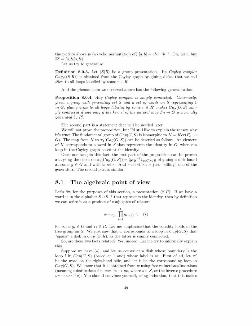
The second part is a statement that will be needed later.We will not prove the proposition, but I’d still like to explain the reason why

it’s true: The fundamental group of Cay(G,S) is isomorphic to K = Ker(FS →G). The map from K to π1(Cay(G,S)) can be descried as follows. An elementof K corresponds to a word in S that represents the identity in G, whence aloop in the Cayley graph based at the identity.

Once one accepts this fact, the first part of the proposition can be provenanalysing the effect on π1(Cay(G,S)) = 〈grg−1〉g∈G,r∈R of gluing a disk basedat some g ∈ G and with label r. And such effect is just “killing” one of thegenerators. The second part is similar.

8.1 The algebraic point of view

Let’s fix, for the purposes of this section, a presentation 〈S|R〉. If we have aword w in the alphabet S ∪ S−1 that represents the identity, then by definitionwe can write it as a product of conjugates of relators:

w =FS

k∏i=1

girig−1i , (∗)

for some gi ∈ G and ri ∈ R. Let me emphasise that the equality holds in thefree group on S. We just saw that w corresponds to a loop in Cay(G,S) that“spans” a disk in Cayc(S,R), as the latter is simply connected.

So, are these two facts related? Yes, indeed! Let me try to informally explainthis.

Suppose we have (∗), and let us construct a disk whose boundary is theloop l in Cay(G,S) (based at 1 and) whose label is w. First of all, let w′

be the word on the right-hand side, and let l′ be the corresponding loop inCay(G,S). We know that it is obtained from w using free reductions/insertions(meaning substitutions like uss−1v → uv, where s ∈ S, or the inverse procedureuv → uss−1v). You should convince yourself, using induction, that this makes

49

l and l′ homotopic, meaning that there is an annulus whose outer circle mapsto l and inner circle maps to l′. So, we now wish to fill w′ instead of w. This ispossible because the loop corresponding to each term girig

−1i looks like Figure

8.1.

Figure 8.1

By the definition of the Cayley complex, there is a disk filling the loop inthe picture. Hence, l′ can be filled by a disk whose image, schematically, lookslike Figure 8.2.

Figure 8.2

The picture is oversimplified, because the loops and sisk can overlap, andwill in general.

This was a brief explanation about how from (∗) one gets a map from a diskin Cayc(S,R). Let us now consider a “nice” disk in Cayc(S,R), meaning onewhose image is naturally tiled by the tiles of Cayc(S,R), as in Figure 8.3:

Let us consider an “external tile”, as in the picture. The important thing tonotice is that the labels of the loops l1 and l2 differ by multiplication by grg−1

and free reductions. The loop labelled grg−1 is the green one in the picture, it

50

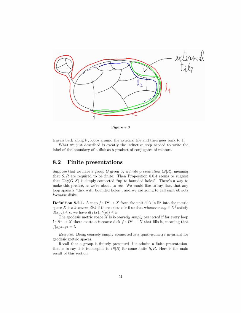
Figure 8.3

travels back along l1, loops around the external tile and then goes back to 1.What we just described is excatly the inductive step needed to write the

label of the boundary of a disk as a product of conjugates of relators.

8.2 Finite presentations

Suppose that we have a group G given by a finite presentation 〈S|R〉, meaningthat S,R are required to be finite. Then Proposition 8.0.4 seems to suggestthat Cay(G,S) is simply-connected “up to bounded holes”. There’s a way tomake this precise, as we’re about to see. We would like to say that that anyloop spans a “disk with bounded holes”, and we are going to call such objectsk-coarse disks.

Definition 8.2.1. A map f : D2 → X from the unit disk in R2 into the metricspace X is a k-coarse disk if there exists ε > 0 so that whenever x.y ∈ D2 satisfyd(x, y) ≤ ε, we have d(f(x), f(y)) ≤ k.

The geodesic metric space X is k-coarsely simply connected if for every loopl : S1 → X there exists a k-coarse disk f : D2 → X that fills it, meaning thatf |∂D2=S1 = l.

Exercise: Being coarsely simply connected is a quasi-isometry invariant forgeodesic metric spaces.

Recall that a group is finitely presented if it admits a finite presentation,that is to say it is isomorphic to 〈S|R〉 for some finite S,R. Here is the mainresult of this section.

51

Theorem 8.2.2. The group G is finitely presented ⇐⇒ one of its Cayleygraphs is coarsely simply connected ⇐⇒ all its Cayley graphs are coarselysimply connected.

The second “⇐⇒ ” is a consequence of the exercise above, which also givesus that:

Corollary 8.2.3. Being finitely presented is a quasi-isometry invariant.

That’s nice, we have an algebraic property that turns out to be a quasi-isometry invariant...

Let us prove the first “⇐⇒ ” of the theorem.

Proof. ⇒: Suppose that G is (isomorphic to) the group given by the finitepresentation 〈S|R〉. We know from Proposition 8.0.4 that the Cayley complexCayc(S,R) is simply connected. Consider now a loop l : S1 → Cay(G,S) (andrecall that we have to show that we can fill it by a coarse disk). There exists acontinuous map f : D2 → Cayc(S,R) that restricts on ∂D2 to l. We can now

construct a new map f : D2 → Cay(G,S) in such a way that if f(x) lies inside

a tile, then f(x) lies on the boundary of the same tile.

It is easy to see that f is a k-coarse disk, where k only depends on themaximal length of a relator in R, which is finite because the presentation isfinite.⇐: Suppose that Cay(G,S) is k-coarsely simply connected. Let R be the

set of labels of all combinatorial simple loops in Cay(G,S) of length at most10k + 10. We claim that 〈S|R〉 is a presentation for G. By the second part ofProposition 8.0.4, what we need to show is that when we glue disks to all simpleloops in Cay(G,S) as above, we get a simply connected space X.

It is enough to check that combinatorial loops in X span disks, because thefundamental group of X is generated by (elements represented by) combinatorialloops.

Let l be a combinatorial loop in Cay(G,S) and let f : D2 → Cay(G,S) be ak-coarse disk that fills it. We have to turn this coarse disk in Cay(G,S) into acontinuous disk g in Cayc(S,R), by “filling in the holes”. Let us triangulate D2

in a sufficiently fine way, and let us perturb f to assume that the image of verticesin such triangulation are vertices of Cay(G,S). Let us now define a continuousmap g : D2 → Cayc(S,R). First of all, g coincides with f on ∂D2 and on thevertices of the triangulation. On each edge contained in the interior of D2, g isa geodesic. To show that the map we defined can be extended to the whole ofD2 we now only need to convince ourselves that the loop obtained restrictingg to the boundary of a triangle of the triangulation is homotopically trivial inCayc(S,R). This follows from easily checked fact that the length of such loopis at most 10k + 10 (if the triangulation we started with was fine enough). Wenow that simple loops of length bounded by 10k + 10 are homotopically trivialin Cayc(S,R), but it’s not hard to see that this implies that all loops with thesame length bound are homotopically trivial as well.

52

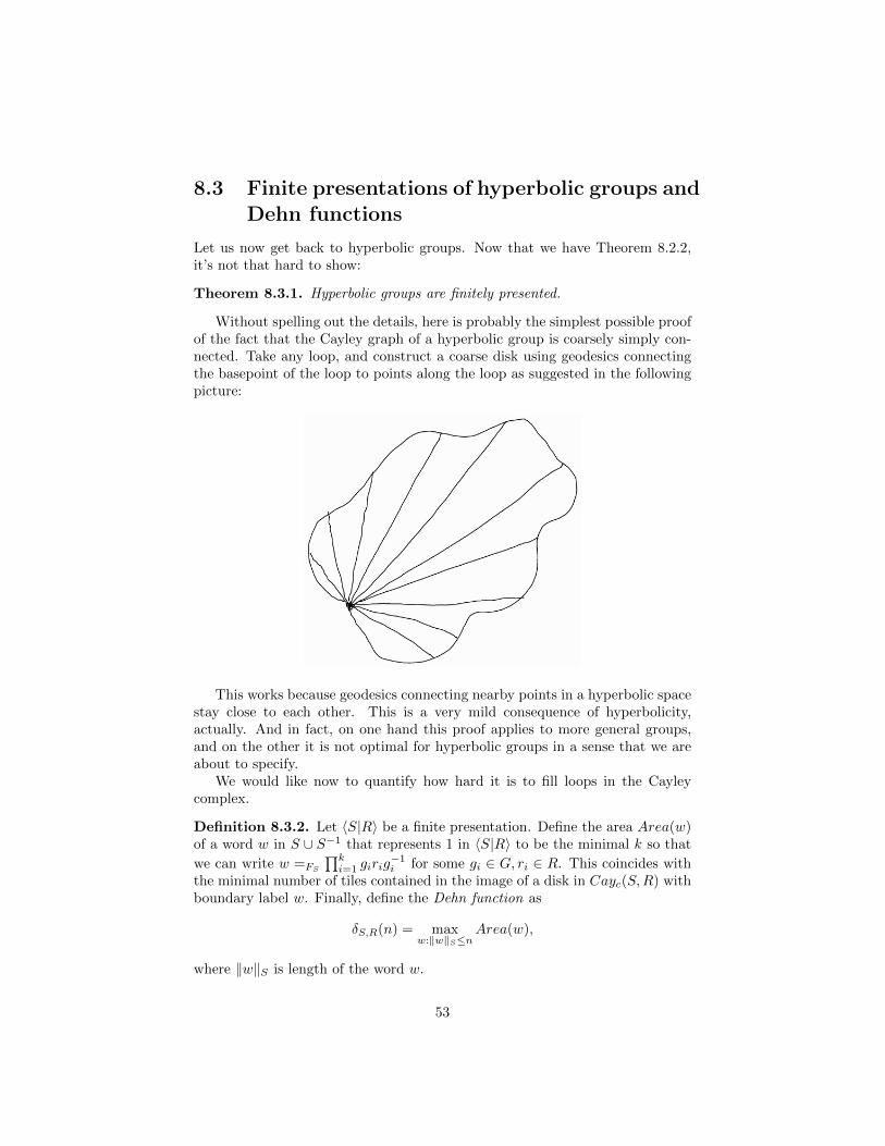
8.3 Finite presentations of hyperbolic groups andDehn functions

Let us now get back to hyperbolic groups. Now that we have Theorem 8.2.2,it’s not that hard to show:

Theorem 8.3.1. Hyperbolic groups are finitely presented.

Without spelling out the details, here is probably the simplest possible proofof the fact that the Cayley graph of a hyperbolic group is coarsely simply con-nected. Take any loop, and construct a coarse disk using geodesics connectingthe basepoint of the loop to points along the loop as suggested in the followingpicture:

This works because geodesics connecting nearby points in a hyperbolic spacestay close to each other. This is a very mild consequence of hyperbolicity,actually. And in fact, on one hand this proof applies to more general groups,and on the other it is not optimal for hyperbolic groups in a sense that we areabout to specify.

We would like now to quantify how hard it is to fill loops in the Cayleycomplex.

Definition 8.3.2. Let 〈S|R〉 be a finite presentation. Define the area Area(w)of a word w in S ∪ S−1 that represents 1 in 〈S|R〉 to be the minimal k so that

we can write w =FS

∏ki=1 girig

−1i for some gi ∈ G, ri ∈ R. This coincides with

the minimal number of tiles contained in the image of a disk in Cayc(S,R) withboundary label w. Finally, define the Dehn function as

δS,R(n) = maxw:‖w‖S≤n

Area(w),

where ‖w‖S is length of the word w.

53

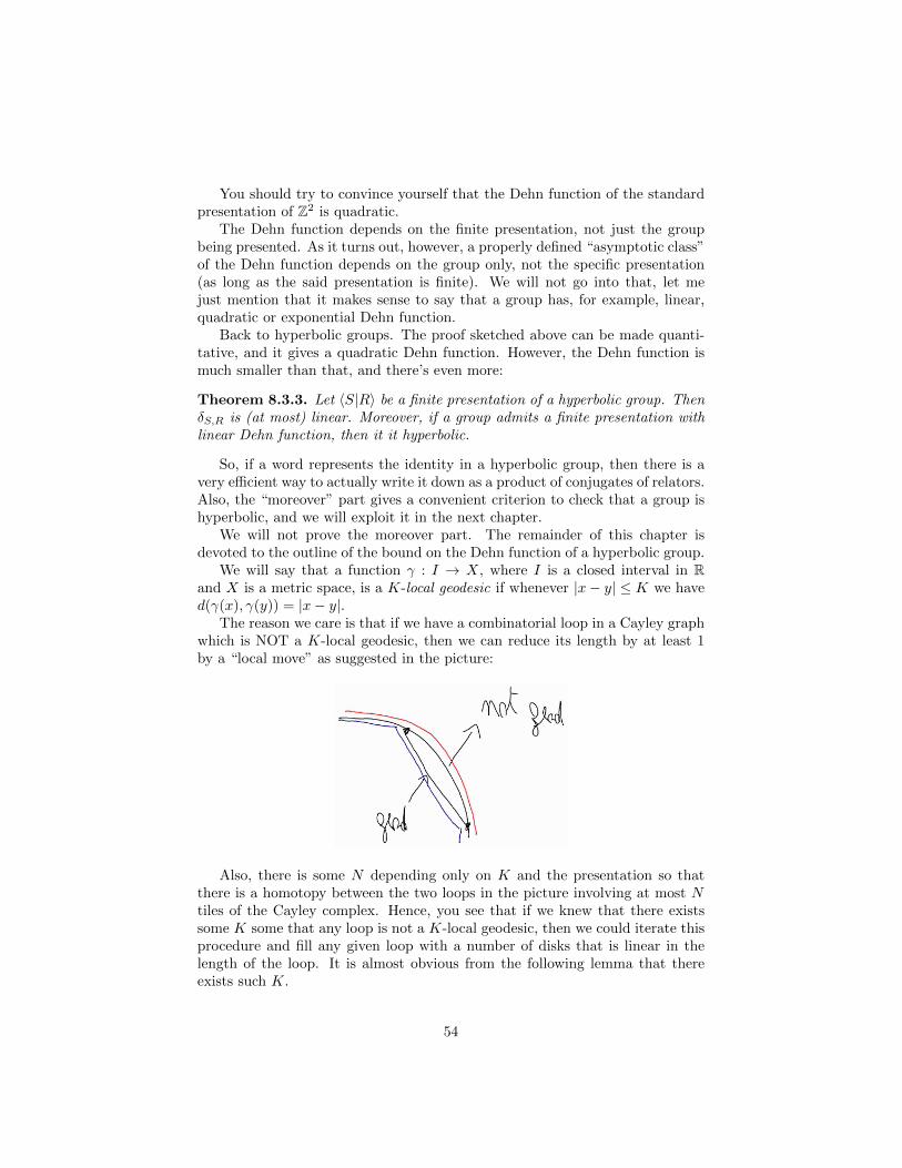
You should try to convince yourself that the Dehn function of the standardpresentation of Z2 is quadratic.

The Dehn function depends on the finite presentation, not just the groupbeing presented. As it turns out, however, a properly defined “asymptotic class”of the Dehn function depends on the group only, not the specific presentation(as long as the said presentation is finite). We will not go into that, let mejust mention that it makes sense to say that a group has, for example, linear,quadratic or exponential Dehn function.

Back to hyperbolic groups. The proof sketched above can be made quanti-tative, and it gives a quadratic Dehn function. However, the Dehn function ismuch smaller than that, and there’s even more:

Theorem 8.3.3. Let 〈S|R〉 be a finite presentation of a hyperbolic group. ThenδS,R is (at most) linear. Moreover, if a group admits a finite presentation withlinear Dehn function, then it it hyperbolic.

So, if a word represents the identity in a hyperbolic group, then there is avery efficient way to actually write it down as a product of conjugates of relators.Also, the “moreover” part gives a convenient criterion to check that a group ishyperbolic, and we will exploit it in the next chapter.

We will not prove the moreover part. The remainder of this chapter isdevoted to the outline of the bound on the Dehn function of a hyperbolic group.

We will say that a function γ : I → X, where I is a closed interval in Rand X is a metric space, is a K-local geodesic if whenever |x− y| ≤ K we haved(γ(x), γ(y)) = |x− y|.

The reason we care is that if we have a combinatorial loop in a Cayley graphwhich is NOT a K-local geodesic, then we can reduce its length by at least 1by a “local move” as suggested in the picture:

Also, there is some N depending only on K and the presentation so thatthere is a homotopy between the two loops in the picture involving at most Ntiles of the Cayley complex. Hence, you see that if we knew that there existssome K some that any loop is not a K-local geodesic, then we could iterate thisprocedure and fill any given loop with a number of disks that is linear in thelength of the loop. It is almost obvious from the following lemma that thereexists such K.

54

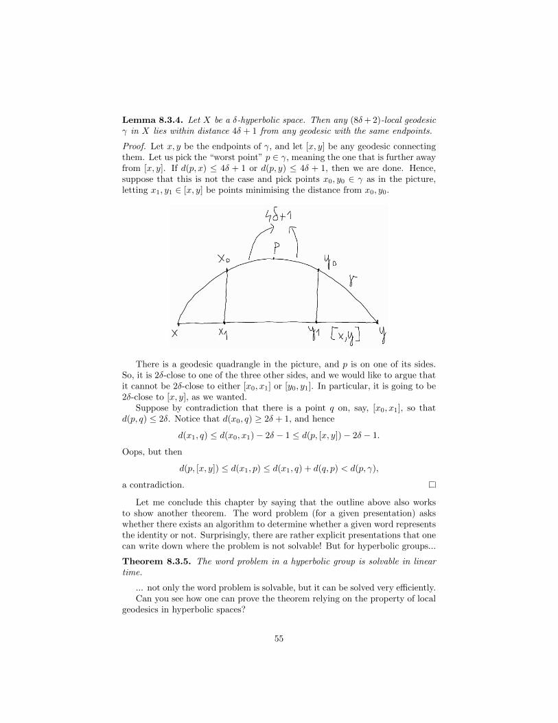
Lemma 8.3.4. Let X be a δ-hyperbolic space. Then any (8δ+ 2)-local geodesicγ in X lies within distance 4δ + 1 from any geodesic with the same endpoints.

Proof. Let x, y be the endpoints of γ, and let [x, y] be any geodesic connectingthem. Let us pick the “worst point” p ∈ γ, meaning the one that is further awayfrom [x, y]. If d(p, x) ≤ 4δ + 1 or d(p, y) ≤ 4δ + 1, then we are done. Hence,suppose that this is not the case and pick points x0, y0 ∈ γ as in the picture,letting x1, y1 ∈ [x, y] be points minimising the distance from x0, y0.

There is a geodesic quadrangle in the picture, and p is on one of its sides.So, it is 2δ-close to one of the three other sides, and we would like to argue thatit cannot be 2δ-close to either [x0, x1] or [y0, y1]. In particular, it is going to be2δ-close to [x, y], as we wanted.

Suppose by contradiction that there is a point q on, say, [x0, x1], so thatd(p, q) ≤ 2δ. Notice that d(x0, q) ≥ 2δ + 1, and hence

d(x1, q) ≤ d(x0, x1)− 2δ − 1 ≤ d(p, [x, y])− 2δ − 1.

Oops, but then

d(p, [x, y]) ≤ d(x1, p) ≤ d(x1, q) + d(q, p) < d(p, γ),

a contradiction.

Let me conclude this chapter by saying that the outline above also worksto show another theorem. The word problem (for a given presentation) askswhether there exists an algorithm to determine whether a given word representsthe identity or not. Surprisingly, there are rather explicit presentations that onecan write down where the problem is not solvable! But for hyperbolic groups...

Theorem 8.3.5. The word problem in a hyperbolic group is solvable in lineartime.

... not only the word problem is solvable, but it can be solved very efficiently.Can you see how one can prove the theorem relying on the property of local

geodesics in hyperbolic spaces?

55

Chapter 9

Small cancellation

In this chapter we construct examples of hyperbolic groups. As it turns out,there is an easy-to-check and widely applicable criterion for a presentation togive a hyperbolic group.

Roughly speaking, the criterion is that common subwords of distinct relatorsshould be short compared to the length of the relators themselves. We will givethe formal definition after we setup some language.

Let S be a finite set, and denote by W (S) the set of all words in the alphabetS ∪ S−1. A subset R ⊆W (S) is said to be symmetrised if

• each w ∈ R is a reduced word,

• if w ∈ R, then w−1 is in R as well,

• if w ∈ R, then all its cyclic shifts are in R as well.

The last item means that if w can be written as avb, then bav is also in R(in particular, it is reduced). Notice that the elements of the free group on Scorresponding to avb and bav are conjugate, as avb =FS b

−1(bav)b.

Definition 9.0.6. Fix some R ⊆ W (S). A piece is a word w ∈ W (S) thatappears as an initial subword of two distinct words in R.

For example, if R = {a2b, a3}, then a and a2 are pieces, but a3 is not.Finally, here is the key definition.

Definition 9.0.7. A symmetrised collection of words R ⊆W (S) satisfies C ′(λ),where λ > 0, if for each r ∈ R and each piece w that appears as a subword of rwe have ‖w‖S < λ‖r‖S .

56

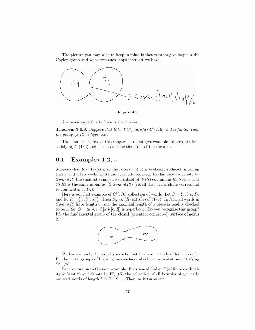
The picture you may wish to keep in mind is that relators give loops in theCayley graph and when two such loops intersect we have:

Figure 9.1

And even more finally, here is the theorem.

Theorem 9.0.8. Suppose that R ⊆W (S) satisfies C ′(1/6) and is finite. Thenthe group 〈S|R〉 is hyperbolic.

The plan for the rest of this chapter is to first give examples of presentationssatisfying C ′(1/6) and then to outline the proof of the theorem.

9.1 Examples 1,2,...

Suppose that R ⊆ W (S) is so that every r ∈ R is cyclically reduced, meaningthat r and all its cyclic shifts are cyclically reduced. In this case we denote bySymm(R) the smallest symmetrised subset of W (S) containing R. Notice that〈S|R〉 is the same group as 〈S|Symm(R)〉 (recall that cyclic shifts correspondto conjugates in FS).

Here is our first example of C ′(1/6) collection of words. Let S = {a, b, c, d},and let R = {[a, b][c, d]}. Then Symm(R) satisfies C ′(1/6). In fact, all words inSymm(R) have length 8, and the maximal length of a piece is readily checkedto be 1. So, G = 〈a, b, c, d|[a, b][c, d]〉 is hyperbolic. Do you recognise this group?It’s the fundamental group of the closed (oriented, connected) surface of genus2.

We knew already that G is hyperbolic, but this is an entirely different proof...Fundamental groups of higher genus surfaces also have presentations satisfyingC ′(1/6).

Let us move on to the next example. Fix some alphabet S (of finite cardinal-ity at least 2) and denote by Wk,l(S) the collection of all k-tuples of cyclicallyreduced words of length l in S ∪ S−1. Then, as it turns out,

57

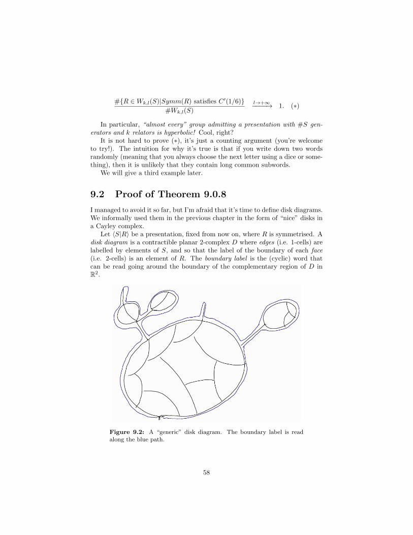
#{R ∈Wk,l(S)|Symm(R) satisfies C ′(1/6)}#Wk,l(S)

l→+∞−−−−→ 1. (∗)

In particular, “almost every” group admitting a presentation with #S gen-erators and k relators is hyperbolic! Cool, right?

It is not hard to prove (∗), it’s just a counting argument (you’re welcometo try!). The intuition for why it’s true is that if you write down two wordsrandomly (meaning that you always choose the next letter using a dice or some-thing), then it is unlikely that they contain long common subwords.

We will give a third example later.

9.2 Proof of Theorem 9.0.8

I managed to avoid it so far, but I’m afraid that it’s time to define disk diagrams.We informally used them in the previous chapter in the form of “nice” disks ina Cayley complex.

Let 〈S|R〉 be a presentation, fixed from now on, where R is symmetrised. Adisk diagram is a contractible planar 2-complex D where edges (i.e. 1-cells) arelabelled by elements of S, and so that the label of the boundary of each face(i.e. 2-cells) is an element of R. The boundary label is the (cyclic) word thatcan be read going around the boundary of the complementary region of D inR2.

Figure 9.2: A “generic” disk diagram. The boundary label is readalong the blue path.

58

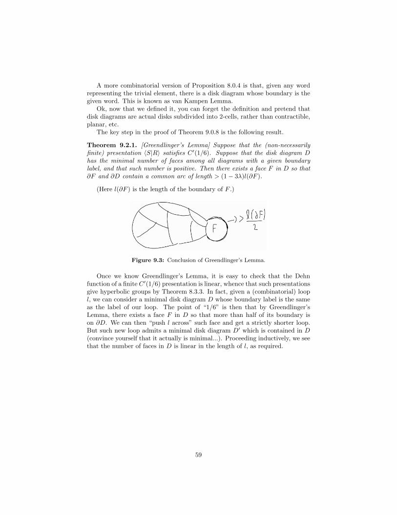
A more combinatorial version of Proposition 8.0.4 is that, given any wordrepresenting the trivial element, there is a disk diagram whose boundary is thegiven word. This is known as van Kampen Lemma.

Ok, now that we defined it, you can forget the definition and pretend thatdisk diagrams are actual disks subdivided into 2-cells, rather than contractible,planar, etc.

The key step in the proof of Theorem 9.0.8 is the following result.

Theorem 9.2.1. [Greendlinger’s Lemma] Suppose that the (non-necessarilyfinite) presentation 〈S|R〉 satisfies C ′(1/6). Suppose that the disk diagram Dhas the minimal number of faces among all diagrams with a given boundarylabel, and that such number is positive. Then there exists a face F in D so that∂F and ∂D contain a common arc of length > (1− 3λ)l(∂F ).

(Here l(∂F ) is the length of the boundary of F .)

Figure 9.3: Conclusion of Greendlinger’s Lemma.

Once we know Greendlinger’s Lemma, it is easy to check that the Dehnfunction of a finite C ′(1/6) presentation is linear, whence that such presentationsgive hyperbolic groups by Theorem 8.3.3. In fact, given a (combinatorial) loopl, we can consider a minimal disk diagram D whose boundary label is the sameas the label of our loop. The point of “1/6” is then that by Greendlinger’sLemma, there exists a face F in D so that more than half of its boundary ison ∂D. We can then “push l across” such face and get a strictly shorter loop.But such new loop admits a minimal disk diagram D′ which is contained in D(convince yourself that it actually is minimal...). Proceeding inductively, we seethat the number of faces in D is linear in the length of l, as required.

59

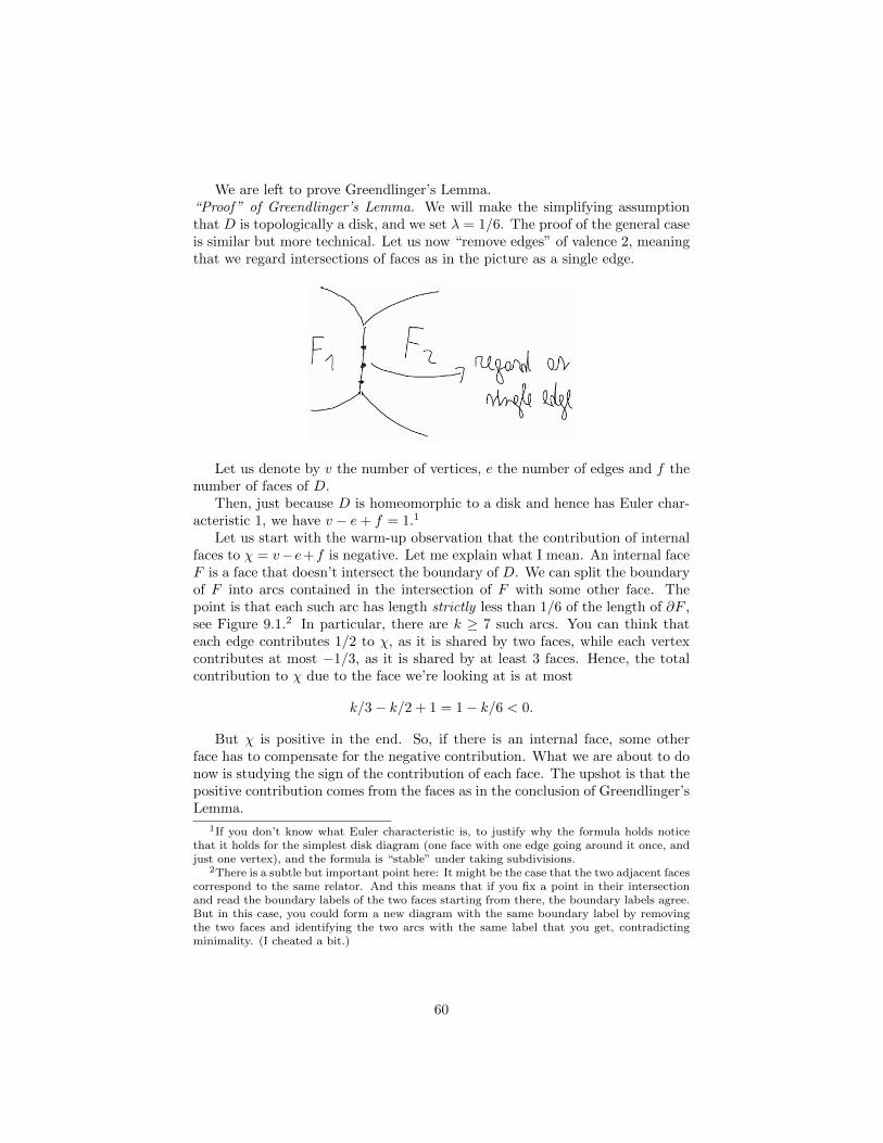
We are left to prove Greendlinger’s Lemma.“Proof” of Greendlinger’s Lemma. We will make the simplifying assumptionthat D is topologically a disk, and we set λ = 1/6. The proof of the general caseis similar but more technical. Let us now “remove edges” of valence 2, meaningthat we regard intersections of faces as in the picture as a single edge.

Let us denote by v the number of vertices, e the number of edges and f thenumber of faces of D.

Then, just because D is homeomorphic to a disk and hence has Euler char-acteristic 1, we have v − e+ f = 1.1

Let us start with the warm-up observation that the contribution of internalfaces to χ = v−e+f is negative. Let me explain what I mean. An internal faceF is a face that doesn’t intersect the boundary of D. We can split the boundaryof F into arcs contained in the intersection of F with some other face. Thepoint is that each such arc has length strictly less than 1/6 of the length of ∂F ,see Figure 9.1.2 In particular, there are k ≥ 7 such arcs. You can think thateach edge contributes 1/2 to χ, as it is shared by two faces, while each vertexcontributes at most −1/3, as it is shared by at least 3 faces. Hence, the totalcontribution to χ due to the face we’re looking at is at most

k/3− k/2 + 1 = 1− k/6 < 0.

But χ is positive in the end. So, if there is an internal face, some otherface has to compensate for the negative contribution. What we are about to donow is studying the sign of the contribution of each face. The upshot is that thepositive contribution comes from the faces as in the conclusion of Greendlinger’sLemma.

1If you don’t know what Euler characteristic is, to justify why the formula holds noticethat it holds for the simplest disk diagram (one face with one edge going around it once, andjust one vertex), and the formula is “stable” under taking subdivisions.

2There is a subtle but important point here: It might be the case that the two adjacent facescorrespond to the same relator. And this means that if you fix a point in their intersectionand read the boundary labels of the two faces starting from there, the boundary labels agree.But in this case, you could form a new diagram with the same boundary label by removingthe two faces and identifying the two arcs with the same label that you get, contradictingminimality. (I cheated a bit.)

60

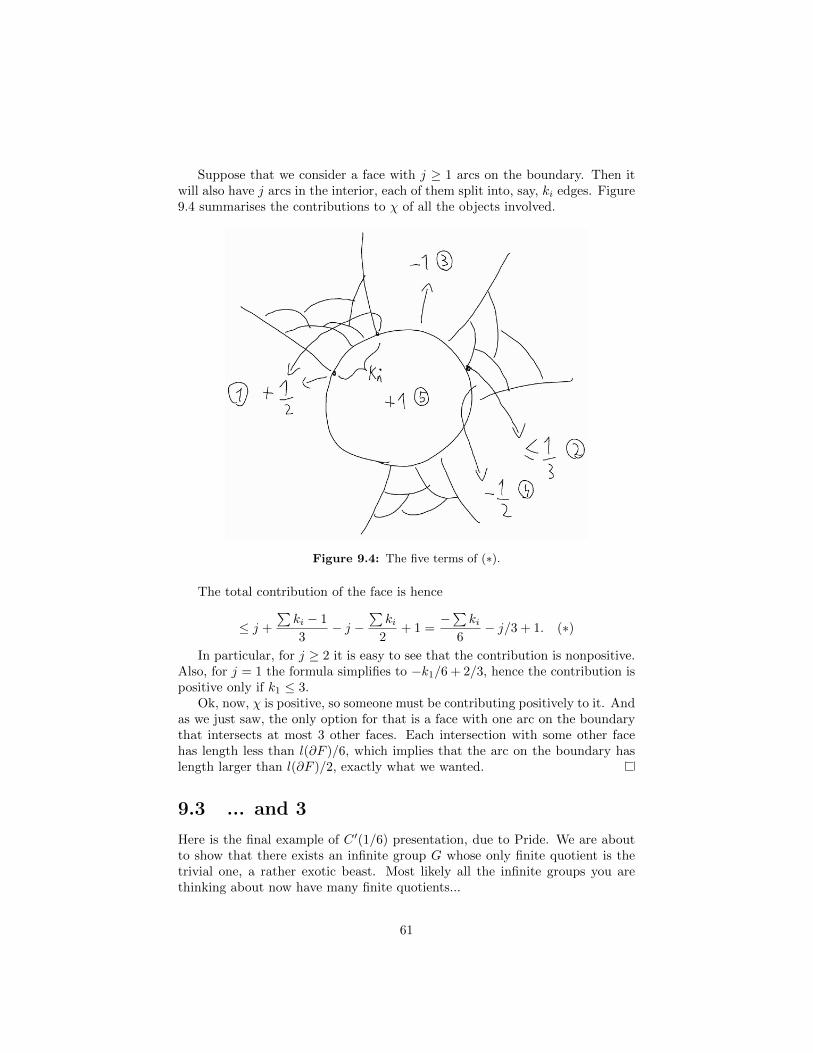
Suppose that we consider a face with j ≥ 1 arcs on the boundary. Then itwill also have j arcs in the interior, each of them split into, say, ki edges. Figure9.4 summarises the contributions to χ of all the objects involved.

Figure 9.4: The five terms of (∗).

The total contribution of the face is hence

≤ j +

∑ki − 1

3− j −

∑ki

2+ 1 =

−∑ki

6− j/3 + 1. (∗)

In particular, for j ≥ 2 it is easy to see that the contribution is nonpositive.Also, for j = 1 the formula simplifies to −k1/6 + 2/3, hence the contribution ispositive only if k1 ≤ 3.

Ok, now, χ is positive, so someone must be contributing positively to it. Andas we just saw, the only option for that is a face with one arc on the boundarythat intersects at most 3 other faces. Each intersection with some other facehas length less than l(∂F )/6, which implies that the arc on the boundary haslength larger than l(∂F )/2, exactly what we wanted.

9.3 ... and 3

Here is the final example of C ′(1/6) presentation, due to Pride. We are aboutto show that there exists an infinite group G whose only finite quotient is thetrivial one, a rather exotic beast. Most likely all the infinite groups you arethinking about now have many finite quotients...

61

Let ui, vi, for i ≥ 1, be words in ai, bi. Let G be given by the presentation〈a, b|{aui, bvi}i≥1〉. We claim that G has no non-trivial finite quotients. In fact,let φ : G → F be a surjective homomorphism onto a finite group. Then thereexists n (e.g. n = |F |) so that φ(an) = φ(bn) = 1. But then φ(un) = φ(vn) = 1,which in turn implies that φ(a) = φ(b) = 1. So, the image of G, which coincideswith F , must be trivial.

Ok, but now... Is G infinite? Maybe we just wrote down a very complicatedpresentation of the trivial group, who knows. Let me remark that there does notexist an algorithm to determine whether a presentation gives the trivial groupor not (!). So, even though it may seem to you that you can probably just sitdown, work a bit and show that for some choice of ui, vi one gets an infinitegroup, this can be trickier than one expects...

But there is a way to guarantee that G is infinite. Suppose that we choosewords ui, vi in such a way that Symm({aui, bvi}) satisfies C ′(1/6), and so that,for each k, ak is never more than half of a relator (such choice is possible). Thenan application of Greendlinger’s Lemma gives that an 6=G 1 for each n ≥ 1, andin particular G is infinite.

Let me conclude this chapter by saying that by studying the C ′(1/6) condi-tion we scratched the surface of the so-called small cancellation theory. Smallcancellation theory has been used extensively to construct exotic groups, andalso to construct interesting quotients of given groups.

62

Chapter 10

Free subgroups

63

Part III

CAT(0) spaces and cubecomplexes

64

Chapter 11

CAT(0) geometry

In this chapter we introduce CAT(0) and nonpositively curved spaces. Nonpos-itively curved spaces are meant to generalise manifolds of nonpositive sectionalcurvature, and CAT(0) spaces their universal covers.

The phenomenon that the definitions capture is that geodesic triangles innonpositive curvature are not “fatter” than geodesic triangles in R2. This holdslocally in nonpositively curved spaces and globally in CAT(0) spaces.

Another good way to think about curvature is that negative curvature forcesgeodesic to diverge rather fast, zero curvature describes the familiar Euclideanspace, while in positive curvature geodesic start off diverging slowly and end upactually converging back together after a while (think of S2, where geodesicsemanating from the north pole are subarcs of longitudes, and hence, when pro-longed, they all end up at the south pole).

11.1 The CAT(0) inequality

Given a triangle ∆ in a metric space, its comparison triangle in R2, denoted ∆is a triangle with the same side lengths as ∆.

Notice that all such triangles are isometric, so we will often talk about thecomparison triangle, with a slight abuse. Also, we will always implictly fix amap φ : ∆ → ∆ which is isometric on the sides of ∆, but to keep the notationcompact, instead of φ(p) we write p. As Figure 11.1 is meant to illustrate, forp a point on ∆ (say not a vertex), p is the point on ∆ so that

• p is on the side γ of ∆ that corresponds to the side γ of ∆ where p lies,and

• the distances from p to the endpoints of γ are the same as the distancesof p from the endpoints of γ.

Definition 11.1.1. A geodesic metric space X is CAT(0) if the following holds.For any geodesic triangle ∆ and p, q ∈ ∆, we have

65

Figure 11.1

dX(p, q) ≤ dR2(p, q). (∗)

A nonpositively curved space is a geodesic metric space which is locallyCAT(0) space, i.e. a space where each point has a neighborhood so that in-equality (∗) holds for triangles contained in that neighborhood.

There is a very useful connection between CAT(0) and nonpositively curvedspaces, via universal covers:

Theorem 11.1.2. If X is nonpositively curved and simply connected, then itis CAT(0). In particular, the universal cover of a nonpositively curved space isCAT(0).

11.2 First examples

The following spaces are CAT(0). We will see more examples (of a more com-binatorial nature) later on.

• Rn. That’s clear, isn’t it?

• Hn. This is less obvious, but still true. And it shouldn’t be too hard tobelieve, I hope...

66

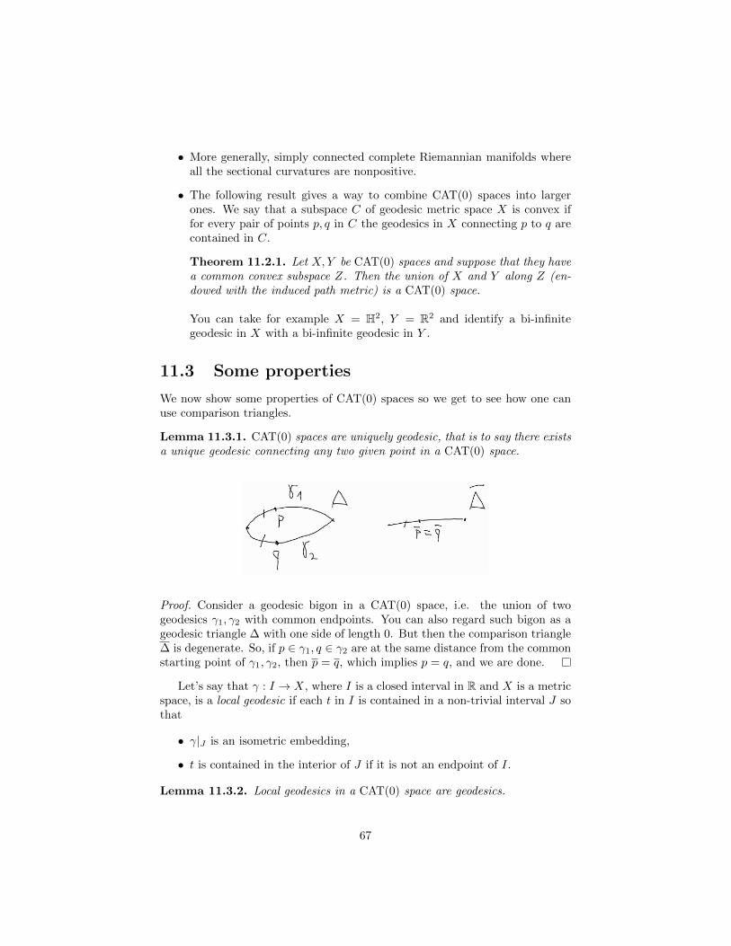
• More generally, simply connected complete Riemannian manifolds whereall the sectional curvatures are nonpositive.

• The following result gives a way to combine CAT(0) spaces into largerones. We say that a subspace C of geodesic metric space X is convex iffor every pair of points p, q in C the geodesics in X connecting p to q arecontained in C.

Theorem 11.2.1. Let X,Y be CAT(0) spaces and suppose that they havea common convex subspace Z. Then the union of X and Y along Z (en-dowed with the induced path metric) is a CAT(0) space.

You can take for example X = H2, Y = R2 and identify a bi-infinitegeodesic in X with a bi-infinite geodesic in Y .

11.3 Some properties

We now show some properties of CAT(0) spaces so we get to see how one canuse comparison triangles.

Lemma 11.3.1. CAT(0) spaces are uniquely geodesic, that is to say there existsa unique geodesic connecting any two given point in a CAT(0) space.

Proof. Consider a geodesic bigon in a CAT(0) space, i.e. the union of twogeodesics γ1, γ2 with common endpoints. You can also regard such bigon as ageodesic triangle ∆ with one side of length 0. But then the comparison triangle∆ is degenerate. So, if p ∈ γ1, q ∈ γ2 are at the same distance from the commonstarting point of γ1, γ2, then p = q, which implies p = q, and we are done.

Let’s say that γ : I → X, where I is a closed interval in R and X is a metricspace, is a local geodesic if each t in I is contained in a non-trivial interval J sothat

• γ|J is an isometric embedding,

• t is contained in the interior of J if it is not an endpoint of I.

Lemma 11.3.2. Local geodesics in a CAT(0) space are geodesics.

67

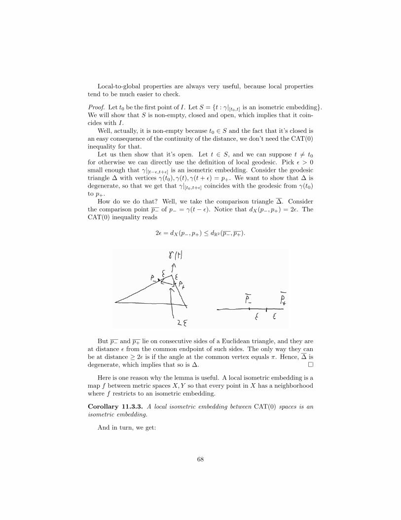
Local-to-global properties are always very useful, because local propertiestend to be much easier to check.

Proof. Let t0 be the first point of I. Let S = {t : γ|[t0,t] is an isometric embedding}.We will show that S is non-empty, closed and open, which implies that it coin-cides with I.

Well, actually, it is non-empty because t0 ∈ S and the fact that it’s closed isan easy consequence of the continuity of the distance, we don’t need the CAT(0)inequality for that.

Let us then show that it’s open. Let t ∈ S, and we can suppose t 6= t0for otherwise we can directly use the definition of local geodesic. Pick ε > 0small enough that γ|[t−ε,t+ε] is an isometric embedding. Consider the geodesictriangle ∆ with vertices γ(t0), γ(t), γ(t + ε) = p+. We want to show that ∆ isdegenerate, so that we get that γ|[t0,t+ε] coincides with the geodesic from γ(t0)to p+.

How do we do that? Well, we take the comparison triangle ∆. Considerthe comparison point p− of p− = γ(t − ε). Notice that dX(p−, p+) = 2ε. TheCAT(0) inequality reads

2ε = dX(p−, p+) ≤ dR2(p−, p+).

But p− and p+ lie on consecutive sides of a Euclidean triangle, and they areat distance ε from the common endpoint of such sides. The only way they canbe at distance ≥ 2ε is if the angle at the common vertex equals π. Hence, ∆ isdegenerate, which implies that so is ∆.

Here is one reason why the lemma is useful. A local isometric embedding is amap f between metric spaces X,Y so that every point in X has a neighborhoodwhere f restricts to an isometric embedding.

Corollary 11.3.3. A local isometric embedding between CAT(0) spaces is anisometric embedding.

And in turn, we get:

68

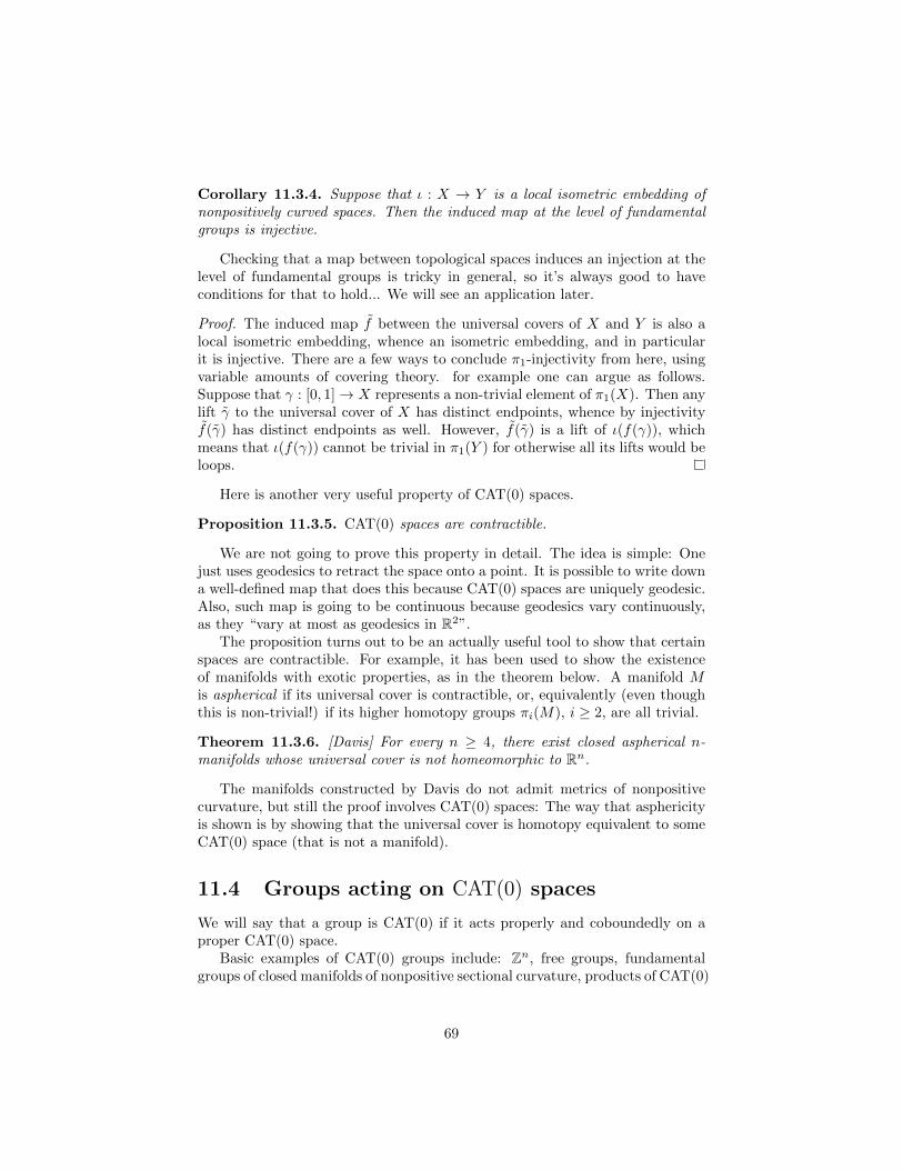
Corollary 11.3.4. Suppose that ι : X → Y is a local isometric embedding ofnonpositively curved spaces. Then the induced map at the level of fundamentalgroups is injective.

Checking that a map between topological spaces induces an injection at thelevel of fundamental groups is tricky in general, so it’s always good to haveconditions for that to hold... We will see an application later.

Proof. The induced map f between the universal covers of X and Y is also alocal isometric embedding, whence an isometric embedding, and in particularit is injective. There are a few ways to conclude π1-injectivity from here, usingvariable amounts of covering theory. for example one can argue as follows.Suppose that γ : [0, 1]→ X represents a non-trivial element of π1(X). Then anylift γ to the universal cover of X has distinct endpoints, whence by injectivityf(γ) has distinct endpoints as well. However, f(γ) is a lift of ι(f(γ)), whichmeans that ι(f(γ)) cannot be trivial in π1(Y ) for otherwise all its lifts would beloops.

Here is another very useful property of CAT(0) spaces.

Proposition 11.3.5. CAT(0) spaces are contractible.

We are not going to prove this property in detail. The idea is simple: Onejust uses geodesics to retract the space onto a point. It is possible to write downa well-defined map that does this because CAT(0) spaces are uniquely geodesic.Also, such map is going to be continuous because geodesics vary continuously,as they “vary at most as geodesics in R2”.

The proposition turns out to be an actually useful tool to show that certainspaces are contractible. For example, it has been used to show the existenceof manifolds with exotic properties, as in the theorem below. A manifold Mis aspherical if its universal cover is contractible, or, equivalently (even thoughthis is non-trivial!) if its higher homotopy groups πi(M), i ≥ 2, are all trivial.

Theorem 11.3.6. [Davis] For every n ≥ 4, there exist closed aspherical n-manifolds whose universal cover is not homeomorphic to Rn.

The manifolds constructed by Davis do not admit metrics of nonpositivecurvature, but still the proof involves CAT(0) spaces: The way that asphericityis shown is by showing that the universal cover is homotopy equivalent to someCAT(0) space (that is not a manifold).

11.4 Groups acting on CAT(0) spaces

We will say that a group is CAT(0) if it acts properly and coboundedly on aproper CAT(0) space.

Basic examples of CAT(0) groups include: Zn, free groups, fundamentalgroups of closed manifolds of nonpositive sectional curvature, products of CAT(0)

69

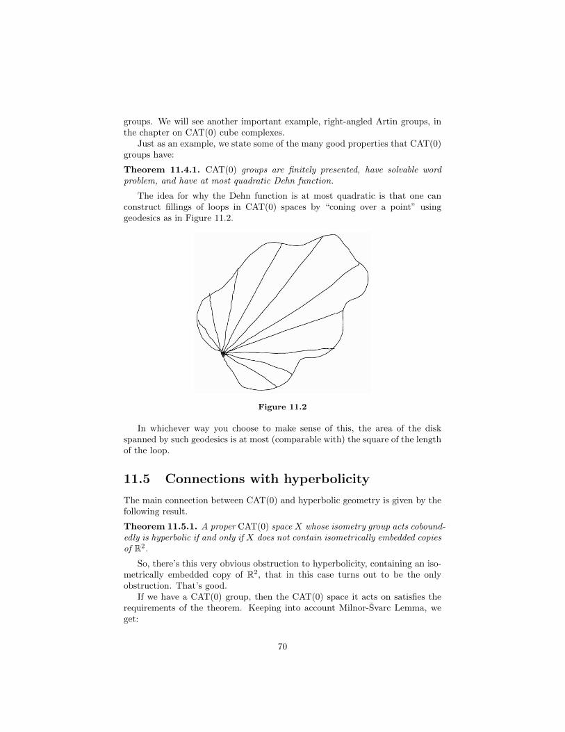
groups. We will see another important example, right-angled Artin groups, inthe chapter on CAT(0) cube complexes.

Just as an example, we state some of the many good properties that CAT(0)groups have:

Theorem 11.4.1. CAT(0) groups are finitely presented, have solvable wordproblem, and have at most quadratic Dehn function.

The idea for why the Dehn function is at most quadratic is that one canconstruct fillings of loops in CAT(0) spaces by “coning over a point” usinggeodesics as in Figure 11.2.

Figure 11.2

In whichever way you choose to make sense of this, the area of the diskspanned by such geodesics is at most (comparable with) the square of the lengthof the loop.

11.5 Connections with hyperbolicity

The main connection between CAT(0) and hyperbolic geometry is given by thefollowing result.

Theorem 11.5.1. A proper CAT(0) space X whose isometry group acts cobound-edly is hyperbolic if and only if X does not contain isometrically embedded copiesof R2.

So, there’s this very obvious obstruction to hyperbolicity, containing an iso-metrically embedded copy of R2, that in this case turns out to be the onlyobstruction. That’s good.

If we have a CAT(0) group, then the CAT(0) space it acts on satisfies therequirements of the theorem. Keeping into account Milnor-Svarc Lemma, weget:

70

Corollary 11.5.2. The CAT(0) group G is hyperbolic if and only if it does notcontain a quasi-isometrically embedded copy of R2.

It is an open question whether or not all hyperbolic groups are CAT(0) (!).Many, probably most people in the field believe that this is not true, though.

Finally, there is also a notion of CAT(−1) space. The definition is similar tothat of a CAT(0) space, except that one considers comparison triangles in H2

instead of R2. Due to the hyperbolicity of H2, CAT(−1) spaces are hyperbolic.

11.6 Nonpositively curved complexes

In this section we consider the followingQuestion: When can one check if a given metric on a compact cell complex

is nonpositively curved?We like compact nonpositively curved cell complexes because their funda-

mental groups are CAT(0), as they act on the universal cover of the cell complex.In general, it is very hard to decide, given a metric celle complex, if it is

nonpositively curved or not. However, there are two classes of examples inwhich nonpositive curvature can be checked easily.

We analyse the first one now, while the second one is the topic of the nextchapter.

Definition 11.6.1. A polygonal complex is a 2-dimensional metric cell complexwhere cells are (isometrically) identified with convex polygons in R2 and the cellsare glued isometrically along sides.

Here are some (topologically planar) examples:

Figure 11.3

Notice that inside the polygons, the local CAT(0) condition is clear becauseany point has a neighborhood isometric to a convex subset of R2. It is also notvery hard to see that there’s no problem in the interior of the edges, as whatyou’re doing there locally is just gluing convex parts of R2 along segments, sothis is fine by Theorem 11.2.1. So, troubles can only happen at vertices.

We are about to define an object, the link, that captures the local geometryaround a vertex, and we will be able to check nonpositive curvature by lookingat links.

71

Let v be a vertex of a polygonal complex. Then the link Lkv at v is themetric graph with

• a vertex corresponding to each half-edge emanating from v,

• edges corresponding to corner of polygons at v,

• the length of each edge equal to the angle (in radians) of the correspondingcorner of polygon.

As usual, pictures are more illuminating:

Figure 11.4

And here we go:

Theorem 11.6.2. A compact polygonal complex is CAT(0) if and only if thelength of any loop in any link is at least 2π.

Here are loops in links from the examples drawn in Figure 11.3 and theirlengths computed under the assumption that all drawn polygons are regular.

Figure 11.5

Notice that all the complexes above are nonpositively curved except for thesecond one. The slogan is “you are nonpositively curved if around each pointthere’s at least as much stuff as in R2”.

Let me try to justify why the condition is sensible, without giving a completeproof.

Let us consider all the (corners of) polygons at a given point that correspondto a loop in the link, and let us add them one by one. When we have only onepolygon, we are fine. Now maybe we have to glue the next one to one side of the

72

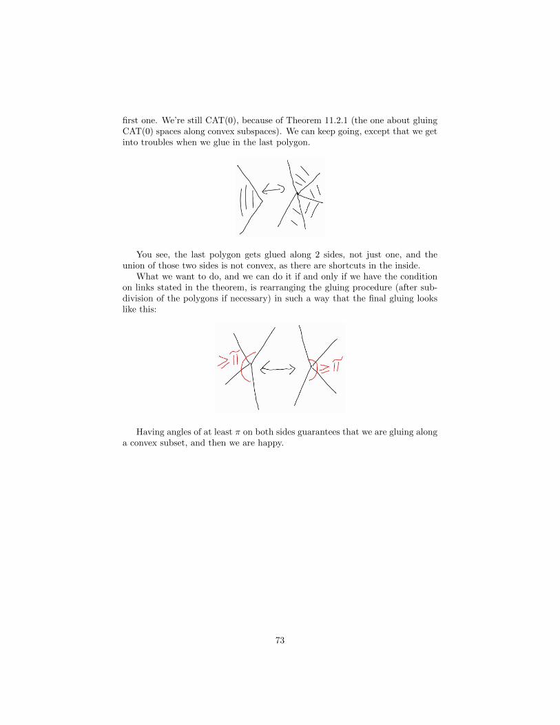
first one. We’re still CAT(0), because of Theorem 11.2.1 (the one about gluingCAT(0) spaces along convex subspaces). We can keep going, except that we getinto troubles when we glue in the last polygon.

You see, the last polygon gets glued along 2 sides, not just one, and theunion of those two sides is not convex, as there are shortcuts in the inside.

What we want to do, and we can do it if and only if we have the conditionon links stated in the theorem, is rearranging the gluing procedure (after sub-division of the polygons if necessary) in such a way that the final gluing lookslike this:

Having angles of at least π on both sides guarantees that we are gluing alonga convex subset, and then we are happy.

73

Chapter 12

CAT(0) cube complexes

A cube complex is just a cell complex obtained gluing Euclidean cubes isomet-rically along faces. As it turns out, it is easy to check when a cube complex isCAT(0) or nonpositively curved (the condition one needs to check has somethingto do with subcomplexes looking like corners of cube actually being corners ofcubes).

The theory of CAT(0) cube complexes is surprisingly rich and goes wellbeyond what one can do with CAT(0) geometry only. In particular, as we willsee, it has been used to prove some big conjectures in low dimensional topology.

12.1 Definitions, nonpositive curvature and flaglinks

Definition 12.1.1. An n-cube is just a copy of [−1, 1]n, endowed with themetric inherited from Rn. A face of an n-cube is the subspace obtained settingone coordinate to either 1 or −1. A cube complex is a metric cell complex whereall cells are (isometric to) n-cubes, and such that the gluing maps are isometriesbetween faces and cubes1.

Figure 12.1: A cube complex

1Yeah, this doesn’t sound right, but it’s the formally correct formulation. It means that the(n− 1)-cells are glued to faces of n-cells. In any case, hopefully the picture is clear enough...

74

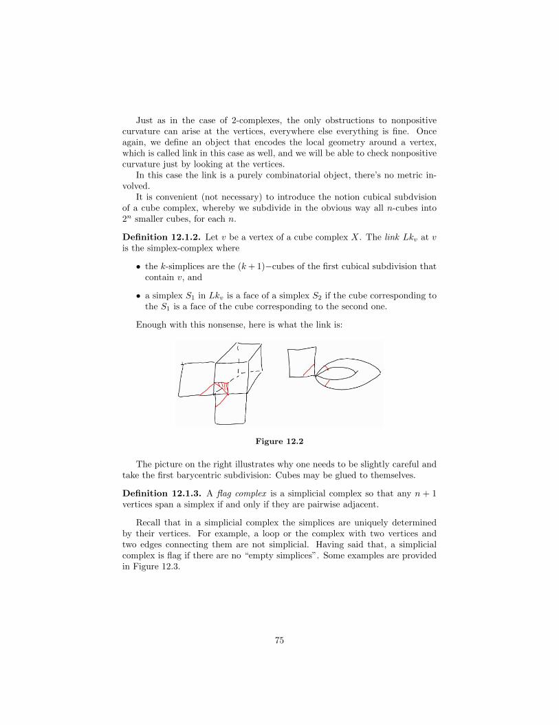
Just as in the case of 2-complexes, the only obstructions to nonpositivecurvature can arise at the vertices, everywhere else everything is fine. Onceagain, we define an object that encodes the local geometry around a vertex,which is called link in this case as well, and we will be able to check nonpositivecurvature just by looking at the vertices.

In this case the link is a purely combinatorial object, there’s no metric in-volved.

It is convenient (not necessary) to introduce the notion cubical subdvisionof a cube complex, whereby we subdivide in the obvious way all n-cubes into2n smaller cubes, for each n.

Definition 12.1.2. Let v be a vertex of a cube complex X. The link Lkv at vis the simplex-complex where

• the k-simplices are the (k+ 1)−cubes of the first cubical subdivision thatcontain v, and

• a simplex S1 in Lkv is a face of a simplex S2 if the cube corresponding tothe S1 is a face of the cube corresponding to the second one.

Enough with this nonsense, here is what the link is:

Figure 12.2

The picture on the right illustrates why one needs to be slightly careful andtake the first barycentric subdivision: Cubes may be glued to themselves.

Definition 12.1.3. A flag complex is a simplicial complex so that any n + 1vertices span a simplex if and only if they are pairwise adjacent.

Recall that in a simplicial complex the simplices are uniquely determinedby their vertices. For example, a loop or the complex with two vertices andtwo edges connecting them are not simplicial. Having said that, a simplicialcomplex is flag if there are no “empty simplices”. Some examples are providedin Figure 12.3.

75

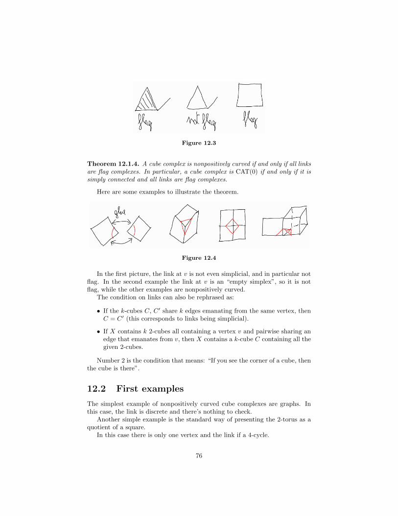
Figure 12.3

Theorem 12.1.4. A cube complex is nonpositively curved if and only if all linksare flag complexes. In particular, a cube complex is CAT(0) if and only if it issimply connected and all links are flag complexes.

Here are some examples to illustrate the theorem.

Figure 12.4

In the first picture, the link at v is not even simplicial, and in particular notflag. In the second example the link at v is an “empty simplex”, so it is notflag, while the other examples are nonpositively curved.

The condition on links can also be rephrased as:

• If the k-cubes C, C ′ share k edges emanating from the same vertex, thenC = C ′ (this corresponds to links being simplicial).

• If X contains k 2-cubes all containing a vertex v and pairwise sharing anedge that emanates from v, then X contains a k-cube C containing all thegiven 2-cubes.

Number 2 is the condition that means: “If you see the corner of a cube, thenthe cube is there”.

12.2 First examples

The simplest example of nonpositively curved cube complexes are graphs. Inthis case, the link is discrete and there’s nothing to check.

Another simple example is the standard way of presenting the 2-torus as aquotient of a square.

In this case there is only one vertex and the link if a 4-cycle.

76

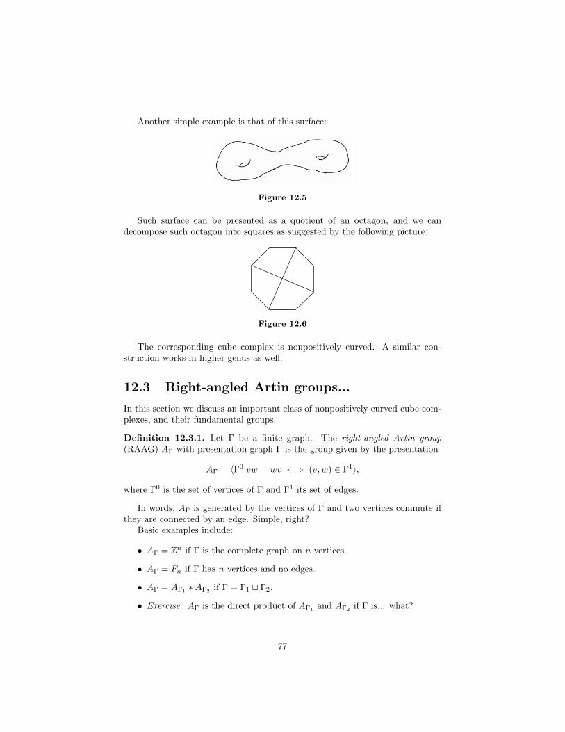
Another simple example is that of this surface:

Figure 12.5

Such surface can be presented as a quotient of an octagon, and we candecompose such octagon into squares as suggested by the following picture:

Figure 12.6

The corresponding cube complex is nonpositively curved. A similar con-struction works in higher genus as well.

12.3 Right-angled Artin groups...

In this section we discuss an important class of nonpositively curved cube com-plexes, and their fundamental groups.

Definition 12.3.1. Let Γ be a finite graph. The right-angled Artin group(RAAG) AΓ with presentation graph Γ is the group given by the presentation

AΓ = 〈Γ0|vw = wv ⇐⇒ (v, w) ∈ Γ1〉,

where Γ0 is the set of vertices of Γ and Γ1 its set of edges.

In words, AΓ is generated by the vertices of Γ and two vertices commute ifthey are connected by an edge. Simple, right?

Basic examples include:

• AΓ = Zn if Γ is the complete graph on n vertices.

• AΓ = Fn if Γ has n vertices and no edges.

• AΓ = AΓ1 ∗AΓ2 if Γ = Γ1 t Γ2.

• Exercise: AΓ is the direct product of AΓ1and AΓ2

if Γ is... what?

77

12.3.1 Salvetti complex

Let us now describe the Salvetti complex SΓ associated to Γ, which is a nonpos-itively curved cube complex whose fundamental group is AΓ.

Start with a bouquet of circles with one loop corresponding to each vertexof Γ:

We also fix an orientation of edge loop. For the moment the fundamentalgroup is just a free group on the vertices of Γ. We now proceed inductively.Whenever v, w are connected by an edge we glue in a 2-cube with the followinggluing instructions:

Notice that opposite edges get glued together and hence the image of thesquare in the Salvetti complex is a 2-torus.

Now we have the right fundamental group, but we might not be nonpositivelycurved yet (there might be “holes” that look like an empty cube). So, wheneverwe have vertices v0, . . . , vk that commute we glue in a k-cube with edges in thei-th direction marked by vi, here is the picture for k = 3:

78

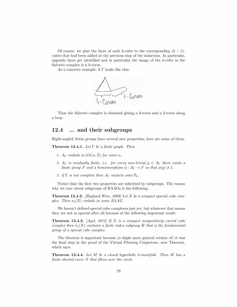
Of course, we glue the faces of such k-cube to the corresponding (k − 1)-cubes that had been added at the previous step of the induction. In particular,opposite faces get identified and in particular the image of the k-cube in theSalvetti complex is a k-torus.

As a concrete example, if Γ looks like this:

Then the Salvetti complex is obtained gluing a 3-torus and a 2-torus alonga loop.

12.4 ... and their subgroups

Right-angled Artin groups have several nice properties, here are some of them.

Theorem 12.4.1. Let Γ be a finite graph. Then

1. AΓ embeds in GL(n,Z) for some n.

2. AΓ is residually finite, i.e. for every non-trivial g ∈ AΓ there exists afinite group F and a homomorphism φ : AΓ → F so that φ(g) 6= 1.

3. if Γ is not complete then AΓ surjects onto F2.

Notice that the first two properties are inherited by subgroups. The reasonwhy we care about subgroups of RAAGs is the following.

Theorem 12.4.2. [Haglund-Wise, 2009] Let X be a compact special cube com-plex. Then π1(X) embeds in some RAAG.

We haven’t defined special cube complexes just yet, but whatever that meansthey are not so special after all because of the following important result:

Theorem 12.4.3. [Agol, 2012] If X is a compact nonpositively curved cubecomplex then π1(X) contains a finite index subgroup H that is the fundamentalgroup of a special cube complex.

The theorem is important because (a slight more general version of) it wasthe final step in the proof of the Virtual Fibering Conjecture, now Theorem,which says:

Theorem 12.4.4. Let M be a closed hyperbolic 3-manifold. Then M has afinite sheeted cover N that fibres over the circle.

79

So, N has the following simple description: Take S × [0, 1], where S is someclosed surface, and glue the boundary components using some homeomorphism.Hence, up to passing to a finite sheeted cover, any closed hyperbolic 3-manifoldadmits such a description.

The proof of the Virtual Fibering Theorem uses a criterion (due to Agol) thatsays, in simplified form, that M virtually fibres over the circle if its fundamentalgroup embeds in some RAAG. Another key step is showing that fundamentalgroups of 3-manifolds can be “cubulated”, so that one can use the two theoremsquoted above.

12.5 Special cube complexes

Time to define special cube complexes. The definition has something to do withthe notion of hyperplane, that we are about to define.

A midcube is the subspace of a cube obtained setting one coordinate to 0.

A hyperplane is, informally speaking, what you get if you start from somemidcubes and keep extending across faces to include other midcubes:

Formally, one defines two edges in a cube complex to be directly parallel ifthey intersect the same midcube, while two edges e, e′ are parallel if there is achain e = e0, . . . , en = e′ of edges so that ei, ei+1 are directly parallel. Finally,a hyperplane is a parallelism class of edges. Not that we really care, of course.

The definition of special cube complex is fine-tuned to make the proof ofTheorem 12.4.2 work. Certain “pathologies” of hyperplanes would prevent theproof from working, and they are exactly the ones that are excluded by thedefinition of specialness. We now give the definition, but you might want toread the proof of Theorem 12.4.2 below instead and come back here when aproperty of hyperplanes is needed in the proof.

80

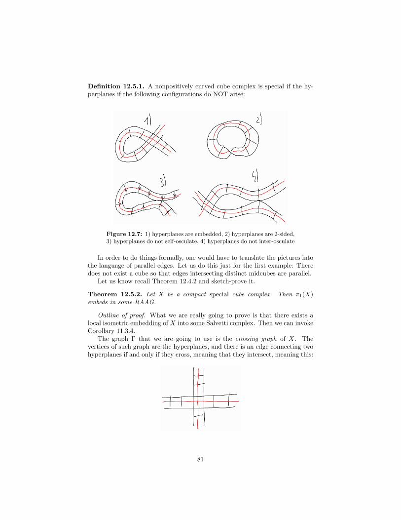
Definition 12.5.1. A nonpositively curved cube complex is special if the hy-perplanes if the following configurations do NOT arise:

Figure 12.7: 1) hyperplanes are embedded, 2) hyperplanes are 2-sided,3) hyperplanes do not self-osculate, 4) hyperplanes do not inter-osculate

In order to do things formally, one would have to translate the pictures intothe language of parallel edges. Let us do this just for the first example: Theredoes not exist a cube so that edges intersecting distinct midcubes are parallel.

Let us know recall Theorem 12.4.2 and sketch-prove it.

Theorem 12.5.2. Let X be a compact special cube complex. Then π1(X)embeds in some RAAG.

Outline of proof. What we are really going to prove is that there exists alocal isometric embedding of X into some Salvetti complex. Then we can invokeCorollary 11.3.4.

The graph Γ that we are going to use is the crossing graph of X. Thevertices of such graph are the hyperplanes, and there is an edge connecting twohyperplanes if and only if they cross, meaning that they intersect, meaning this:

81

As hyperplanes of X are two-sided (property 2), we can orient coherently alledges dual (formally: contained) in a given hyperplane. Just pick any orienta-tion of one edge, put the obivous orientation on all the edges dual to the samemidcube and keep extending.

We are now ready to define a map from the 1-skeleton of X to the 1-skeletonof SΓ, which is just a bouquet of oriented loops each corresponding to a hyper-plane of X.

The map is defined as follows. The image of an edge e of X is the loop in S1Γ

corresponding to the (only) hyperplane dual to e, and e is mapped isometricallyand orientation-preservingly onto such edge.

If this map is going to be a local isometric embedding it’d better be locallyinjective. But what would it mean for two edges in X emanating from the samevertex to be mapped onto the same edge in SΓ? It would mean that two suchedges are contained in the same hyperplane. But this cannot happen for edgescontained in a common square because hyperplanes are embedded (property 1).Also, it cannot happen for edges not contained in a common square because ofno interosculation (property 3). So, it can never happen. (There is a subtletyabout orientation in the second case, can you see it?)

Now, there is a combinatorial characterisation of local isometries. If you arewilling to believe me, what you need to check (once you have local injectivity)is exactly that the following obvious obstruction to being a local isometric em-bedding does not arise at any vertex v: Two edges emanating from v that arenot contained in a common square get mapped to edges contained in a commonsquare. And this is exactly what property 4 prevents.

In order to conclude the proof, one needs to check that the map we definedon the 1-skeleton extends to higher skeleta as well, and we will only mentionthat this uses the flag condition.

82

Chapter 13

Cubulation

In this chapter we describe the most important way to construct CAT(0) cubecomplexes. The main idea is that the structure of a CAT(0) cube complex can isentirely encoded by the combinatorics of its hyperplanes, and in turn the way inwhich hyperplanes cut up a CAT(0) cube complex can be axiomatised in termsof the notion of wall.

In this chapter it will be most convenient to regard a hyperplane as an actualsubspace of the CAT(0) cube complex rather than as a parallelism class of edges,and hence we will do so.

13.1 Properties of hyperplanes

Let us start with stating the main properties of hyperplanes.

Theorem 13.1.1. Let H be a hyperplane in the CAT(0) cube complex X. Then

1. H is embedded,

2. H is convex,

3. X\H has exactly two connected components.

Let me also remark that H is in a natural way a CAT(0) cube complexitself. The dimension of H (meaning the maximal dimension of cubes in H) isstrictly smaller than the dimension of X. This is useful because sometimes itcan be used to prove statements about CAT(0) cube complexes using inductionon dimension.

We are actually not going to use the theorem, but I thought it was worthstating it anyway to motivate what we are going to do.

Just to give an idea about how one can prove (part of) it, let me recallthat local isometric embeddings between CAT(0) spaces are (global) isometricembeddings (Lemma 11.3.3). Hence, you get 1) and 2) if you show that theinclusion of H into X is a local isometric embedding, and this shouldn’t sound

83

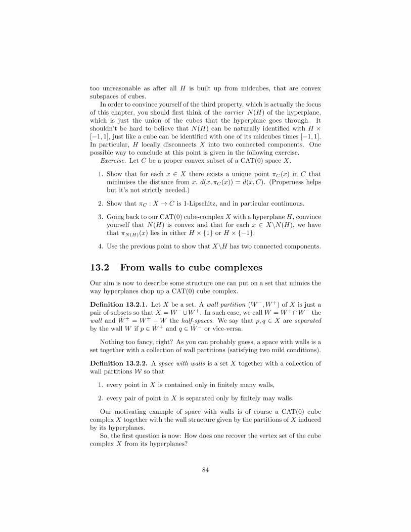
too unreasonable as after all H is built up from midcubes, that are convexsubspaces of cubes.

In order to convince yourself of the third property, which is actually the focusof this chapter, you should first think of the carrier N(H) of the hyperplane,which is just the union of the cubes that the hyperplane goes through. Itshouldn’t be hard to believe that N(H) can be naturally identified with H ×[−1, 1], just like a cube can be identified with one of its midcubes times [−1, 1].In particular, H locally disconnects X into two connected components. Onepossible way to conclude at this point is given in the following exercise.

Exercise. Let C be a proper convex subset of a CAT(0) space X.

1. Show that for each x ∈ X there exists a unique point πC(x) in C thatminimises the distance from x, d(x, πC(x)) = d(x,C). (Properness helpsbut it’s not strictly needed.)

2. Show that πC : X → C is 1-Lipschitz, and in particular continuous.

3. Going back to our CAT(0) cube-complex X with a hyperplane H, convinceyourself that N(H) is convex and that for each x ∈ X\N(H), we havethat πN(H)(x) lies in either H × {1} or H × {−1}.

4. Use the previous point to show that X\H has two connected components.

13.2 From walls to cube complexes

Our aim is now to describe some structure one can put on a set that mimics theway hyperplanes chop up a CAT(0) cube complex.

Definition 13.2.1. Let X be a set. A wall partition (W−,W+) of X is just apair of subsets so that X = W−∪W+. In such case, we call W = W+∩W− thewall and W± = W± −W the half-spaces. We say that p, q ∈ X are separatedby the wall W if p ∈ W+ and q ∈ W− or vice-versa.

Nothing too fancy, right? As you can probably guess, a space with walls is aset together with a collection of wall partitions (satisfying two mild conditions).

Definition 13.2.2. A space with walls is a set X together with a collection ofwall partitions W so that

1. every point in X is contained only in finitely many walls,

2. every pair of point in X is separated only by finitely may walls.

Our motivating example of space with walls is of course a CAT(0) cubecomplex X together with the wall structure given by the partitions of X inducedby its hyperplanes.

So, the first question is now: How does one recover the vertex set of the cubecomplex X from its hyperplanes?

84

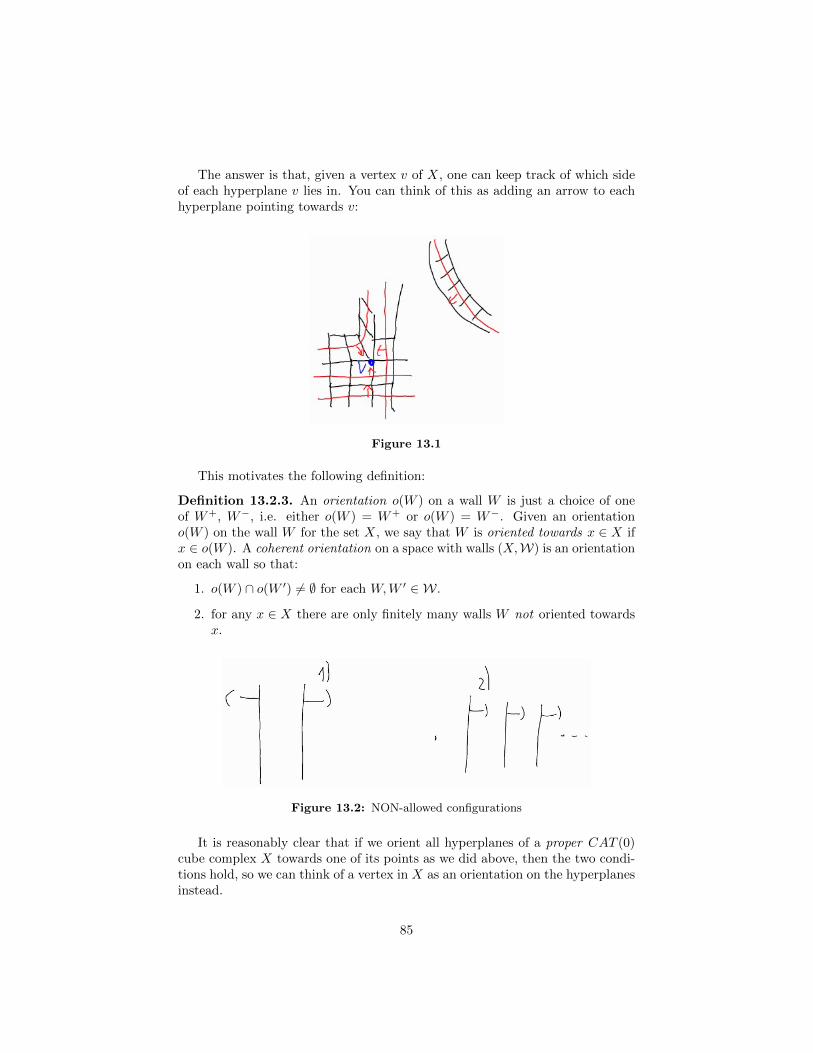
The answer is that, given a vertex v of X, one can keep track of which sideof each hyperplane v lies in. You can think of this as adding an arrow to eachhyperplane pointing towards v:

Figure 13.1

This motivates the following definition:

Definition 13.2.3. An orientation o(W ) on a wall W is just a choice of oneof W+, W−, i.e. either o(W ) = W+ or o(W ) = W−. Given an orientationo(W ) on the wall W for the set X, we say that W is oriented towards x ∈ X ifx ∈ o(W ). A coherent orientation on a space with walls (X,W) is an orientationon each wall so that:

1. o(W ) ∩ o(W ′) 6= ∅ for each W,W ′ ∈ W.

2. for any x ∈ X there are only finitely many walls W not oriented towardsx.

Figure 13.2: NON-allowed configurations

It is reasonably clear that if we orient all hyperplanes of a proper CAT (0)cube complex X towards one of its points as we did above, then the two condi-tions hold, so we can think of a vertex in X as an orientation on the hyperplanesinstead.

85

Now, the last observation: If x, y are vertices of the CAT (0) cube complexX and they are connected by an edge e, then the corresponding orientationsdiffer exactly on one hyperplane, namely the one dual to e.

We now have everything we need to construct a CAT (0) cube complex froma space with walls.

Definition 13.2.4. Let (X,W) be a space with walls. Then its dual cubecomplex C = C(X,W) is the cube complex with

• vertices ↔ coherent orientations on W,

• edges ↔ orientations that differ on exactly one wall, and

• n-cubes ↔ 1-skeleta of n-cubes.

The last item means that we plug in an n-cube wherever we see a subcomplexof the 1-skeleton of C isomorphic to the 1-skeleteon of an n-cube.

And the theorem is...

Theorem 13.2.5 (Sageev). If (X,W) is a space with walls, then its dual cubecomplex is CAT (0).

It is important to remark that the construction of the dual cube complex isnatural in the sense that if (X,W) is a space with walls and you have a groupG acting on X preserving W, then G is going to act on the dual cube complexas well. Hence, the theorem gives a way to construct actions on CAT (0) cubecomplexes.

13.3 Examples

We already discussed the example of cube complexes during the discussion lead-ing to the definition of the dual cube complex, but let us analyse a concreteexample.

1. Consider the standard cubulation of R2. The walls/hyperplanes naturallycome in two families, corresponding to horizontal and vertical lines. Acoherent orientation is uniquely determined by a horizontal and a vertical“switch point”, meaning the following. Suppose that you want a coherentorientation just on the vertical lines, for the moment. You cannot havethe configuration in Figure 13.2-(1).

Also, not all hyperplanes can be oriented in the same direction, for other-wise infinitely many of them will point away from the origin.

This forces the orientation to look like in Figure 13.3.

The switch point is where hyperplanes switch from being oriented to theright to being oriented to the left.

A similar argument applies to the horizontal lines, and you can check thatyou can choose orientations on horizontal and vertical lines independently.

Here are a few more examples.

86

Figure 13.3

2. Let G be the group of symmetries of the tessellation of R2 by equilateraltriangles:

R2 has a G-invariant wall structure W with three families of walls assuggested by the following picture:

In each family of wall an orientation is determined by a “switch point”,and the switch points can be chosen independently, like in the previouscase. Hence, in this case the dual cube complex C is R3 with the standardcubulation.

The action of G on C is proper but cannot possibly be cobounded (G is“2-dimensional” for any meaningful definition of dimension).

Actually, there are conditions for the action on the dual cube complex tobe proper and/or cobounded, but we will not go into this (even thoughit’s very important).

3. Walls in small cancellation groups. Let 〈S|R〉 be a C ′(1/6) presentation,say with all relators of even length for simplicity. Here is an idea toconstruct walls in the Cayley complex. Define a mid-cell to be a line thatgoes from the midpoint of one edge in a relator to the midpoint of theopposite edge.

As it turns out, if you start from a midcell and maximally extend throughthe edges, you get an embedded graph that separates your Cayley complex

87

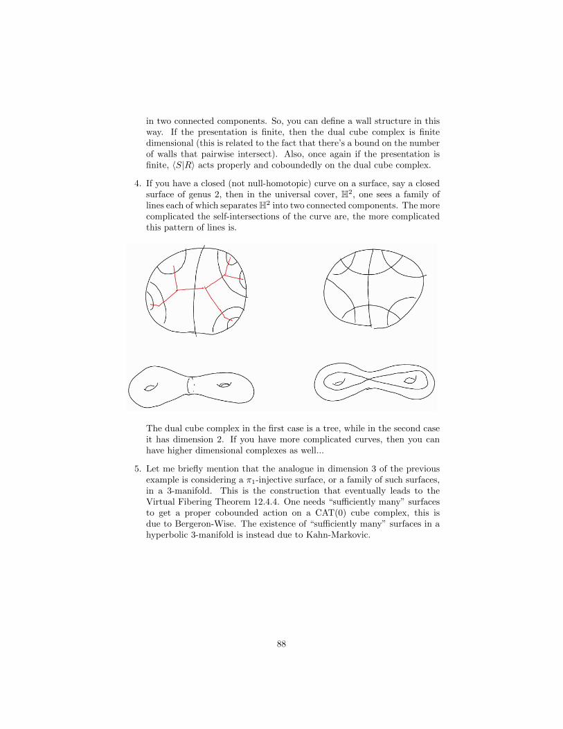
in two connected components. So, you can define a wall structure in thisway. If the presentation is finite, then the dual cube complex is finitedimensional (this is related to the fact that there’s a bound on the numberof walls that pairwise intersect). Also, once again if the presentation isfinite, 〈S|R〉 acts properly and coboundedly on the dual cube complex.

4. If you have a closed (not null-homotopic) curve on a surface, say a closedsurface of genus 2, then in the universal cover, H2, one sees a family oflines each of which separatesH2 into two connected components. The morecomplicated the self-intersections of the curve are, the more complicatedthis pattern of lines is.

The dual cube complex in the first case is a tree, while in the second caseit has dimension 2. If you have more complicated curves, then you canhave higher dimensional complexes as well...

5. Let me briefly mention that the analogue in dimension 3 of the previousexample is considering a π1-injective surface, or a family of such surfaces,in a 3-manifold. This is the construction that eventually leads to theVirtual Fibering Theorem 12.4.4. One needs “sufficiently many” surfacesto get a proper cobounded action on a CAT(0) cube complex, this isdue to Bergeron-Wise. The existence of “sufficiently many” surfaces in ahyperbolic 3-manifold is instead due to Kahn-Markovic.

88