Embed Size (px)
Citation preview

Lecture Notes: “Land Evaluation”
by
David G. Rossiter
Cornell UniversityCollege of Agriculture & Life Sciences
Department of Soil, Crop, & Atmospheric Sciences
August 1994
Part 4: Economic Land Evaluation
Disclaimer: These notes were developed for the Cornell University course Soil,Crop & Atmospheric Sciences 494 ‘Special Topics in Soil, Crop & AtmosphericSciences: Land evaluation, with emphasis on computer applications’, SpringSemester 1994, and were subsequently expanded and formatted for publication.They are not to be considered as a definitive text on land evaluation.
Copyright David G. Rossiter 1994. Complete or partial reproduction ofthese notes is permitted if and only if this note is included. Sale of these notesor any copy is strictly prohibited.

Contents of Part 4 “Economic land evaluation”
1. Introduction to economic land evaluation ........................21.1 Motivation for economic land evaluation ...................21.2 What economics can not analyze................................31.3 Definition of economic suitability ..............................41.4 Determinants of economic suitability.........................41.5 Economic vs. financial analysis..................................41.6 Measures of economic suitability ...............................5
2. Economic land evaluation in ALES .................................102.1 How ALES links land characteristics with economicvalues ............................................................................102.2 ALES approach to location-independent LQs ............102.3 ALES approach to location-dependent LQs ...............142.4 GIS approach to location-dependent LQs..................152.5 Production-related costs ..........................................162.6 Economic suitability classes ....................................16
3. Optimization under constraints by a single manager ......183.1 Why is optimization needed? ...................................183.2 What is being optimized? the objective function ......193.3 Constraints ..............................................................193.4 Mathematical programming .....................................213.5 Formulating the mathematical program ...................213.6 Assumptions of linear programming .........................233.7 Solving the linear programming problem..................243.8 Slack variables .........................................................253.9 Duality and shadow prices........................................253.10 Sensitivity analysis ................................................273.11 Modeling more realistic production scenarios ........283.12 Using the results of ALES evaluations in linear programs ....28
4. Risk analysis..................................................................304.1 Uncertainty, risk, & risk-taking behavior..................314.2 Payoff matrix, expected value, and variance.............324.3 Expressing risk aversion ..........................................334.4 Evaluating risk: mean-variance (E,V) analysis...........344.5 Evaluating risk: the MOTAD model...........................344.6 Evaluating risk: safety-first ......................................354.7 The @RISK software .................................................36
5. Decision theory and multi-objective decision making .....375.1 Definitions...............................................................37

5.2 Kinds of evaluations ................................................385.3 Multi-criteria decision making .................................395.4 Multi-objective decision making...............................40
6. References .....................................................................42

Land Evaluation Course Notes Part 4: Economic Land Evaluation 1
Physical land evaluation provides no objective method to compare different land uses for agiven land area, as there is no inherent common scale of measure between the land uses.We can count the number of physical constraints to each use, but it is difficult to comparetheir relative severity or degree of limitation. Some constraints may lead directly to yieldreductions, but others are only expressed as management difficulties. We need someobjective and commensurate comparison of costs and-benefits for each land use on eachland unit. In many situations, it is realistic to use economic measures of costs andbenefits, and then use these to quantify the land use potential and suitability, accordingto the land evaluation definition.
In this unit we introduce the micro-economic concepts used in land evaluation, payingparticular attention to the way these are used in the ALES computer program. We thendiscuss optimization of land uses under constraints by a single decision maker, and in thewider context of decision theory.

Land Evaluation Course Notes Part 4: Economic Land Evaluation 2
1. Introduction to economic landevaluation
We don’t pretend to survey the vast field of agricultural and natural resourceeconomics, only those aspects that directly bear on the land evaluation process.
References: (Barlowe, 1986) is a basic text on land economics, a moreidiosyncratic view is by (Dovring, 1987). The kind of microeconomic analysispresented here is very similar to the analysis of engineering projects, e.g., thetext of (Newman, 1991). Chapter 9 of the EUROCONSULT agriculturalcompendium (1989) discusses the relative merits of the different economicmeasures of suitability as well as the distinction between economic andfinancial analysis. (Colman & Young, 1989) is a good introduction to theeconomic analysis of the agricultural sector. For a broader policy view ofagriculture and development, see (Ghatak & Ingersent, 1984). (Carlson,Zilberman & Miranowski, 1993) explains the many tricky questions ofenvironmental economics.
1.1 Motivation for economic land evaluation
Historically, land evaluation had its origin in land capability classification, soil surveyinterpretation, and similar physical evaluations, in which the use potential of land isexpressed in terms of its predicted physical response to various land uses or in terms ofphysical constraints to these uses. However, a physical evaluation provides no objectivemethod to compare different land uses for a given land area, as there is no inherentcommon scale of measure between the land uses. We can count the number of physicalconstraints to each use, but it is difficult to compare their relative severity or degree oflimitation. Some constraints may lead directly to yield reductions, but others are onlyexpressed as management difficulties. We need some objective cost-vs.-benefitcomparison.
In general terms, the land user wants maximum benefits with minimum effort, subject to aset of constraints.
Key question: How do we measure the ‘benefits’ and ‘effort’ of this general equation?
In purely subsistence agriculture, the benefits are the consumable foodstuffs, fiber, wood,animal products etc. They can be quantified as calories, grams of protein, etc. The costsare labor, which can be quantified by time and intensity.
In market-oriented societies that are largely organized by economic interactions (i.e., wheremoney and its surrogates are the primary means of exchange) both benefits and costs canbe expressed by economic measures: ‘everything has its price’.

Land Evaluation Course Notes Part 4: Economic Land Evaluation 3
Thus, economic measures are a reasonable way to compare the various use potentials ofland and land uses. The FAO recognized this in its Framework and Guidelines for landevaluation. Their sketchy attempt to provide an economic framework was amplifiedsomewhat by (Dent & Young, 1981) following a study of theirs from Malawi (Young &Goldsmith, 1977). Also, the quasi-economic analysis of the US Bureau of Reclamation’sland classification system (U.S. Department of the Interior, 1951) was a precursor. Arecent outstanding example of economic land evaluation is (Johnson & Cramb, 1991,1992).
1.2 What economics can not analyze
It is certainly true that individuals, groups and societies are not completelymotivated by the desire to make and accumulate wealth, but this does notmean that economic analysis is not valid. All that is really required is thatmoney is acceptable as a means of exchange and that most preferences can begiven a monetary value.
These ‘non-economic’ preferences can be expressed as absolute or partialbarriers to economic behavior. If absolute, they limit the possible LUTs. Ifpartial, they should have an economic cost, which can be obtained by analyzingthe foregone benefits.
Example: a religious dietary prohibition: an absolute barrier would be if theindividual would die rather than eat the prohibited food; a partial barrier wouldbe a more-or-less avoidance of the food but not an absolute prohibition. Wecould measure the degree of avoidance by presenting the individual with arestaurant menu, with the prohibited food valued at $1 and various permittedfoods valued at increasingly higher amounts, then every time they ordered apermitted food, telling them that we were out of that item, until they finallyordered the prohibited food. Similar experiments can be used to give aneconomic value to other preferences.
Example: ties to the land (ancestral village) or preference for a way of life; thesecan be measured by offering ever-higher prices for the land until the landowneragrees to sell.
Another problem with economic analysis is the long-term, or inter-generational,transfer of wealth. Unless some mechanism is in place to ensure that present-day decision makers do not mortgage the future, they may well do just that.
A serious problem and an area of active research is the assignment of economicvalues to things that do not have an established market value in the samesense as an actively-traded good such as a food commodity. Much ofenvironmental economics (Carlson, Zilberman & Miranowski, 1993) is taken upwith this problem. In a land evaluation context, this includes obviousexternalities (off-farm effects) such as water pollution and sedimentation ofreservoirs as well as changes (temporary or irreversible) to the in-situ resourcebase.

Land Evaluation Course Notes Part 4: Economic Land Evaluation 4
1.3 Definition of economic suitability
The economic suitability of a land area for a land use (= Barlowe’s (1986) land usecapacity) is the predicted net economic benefit to a specified party (e.g.,landowner, land user, society) to be expected if the land area is dedicated to theuse.
Note: the economic value of a land use system implemented on a given landarea is not synonymous with the market value of the land area (land evaluation ≠land valuation) although the predicted return to a land unit of various land usesobviously influences its price. (In fact, the price should be at least the greatestNet Present Value of the possible land uses, see below).
This definition begs the question, which we consider below, of how to measurethe net benefit.
1.4 Determinants of economic suitability
Economic suitability depends on three types of factors:
1. The in-situ resource quality, i.e. the response of the land to the use withoutregard to its location (Ricardo). Example: predicted crop yield.
2. The accessibility, and by extension, all costs and benefits associated with thespecific location as opposed to the resource quality (von Thünen). Classicexample: transportation costs for inputs and products.
3. Other spatial attributes of the site, not including accessibility, for example,size, shape, adjacency, and contiguity. Example: more efficient field work ifthe parcel is the correct shape and size/
The evaluation starts from a physical basis, i.e. specific land areas with theirland characteristics expressed quantitatively or qualitatively in physical terms,for example ‘3 to 8%’ or ‘moderate’ slopes (in-situ resource quality), or ‘3 kmfrom the nearest paved road’ (accessibility) or ‘40 ha parcels’ (spatial attributes).It should end with quantitative predictions about economic value, e.g. ‘$240 ±$30 ha-1 yr-1 predicted net return to labor’ or with land allocation based onsuch values. The link between the physical basis (the land) and the economicvalue of the land use is the tricky part.
1.5 Economic vs. financial analysis
Financial analysis: from the point of view of the individual land user (operator): the cashflows (and derived measures) as perceived by the operator, and thus guiding his or herdecision-making. All prices must be real, i.e., as paid/received by the operator. By
Land Evaluation Course Notes Part 4: Economic Land Evaluation 5
definition, externalities are not included, unless they have been assigned a real cost (e.g.,tax credits for low-input farming).
Economic analysis: from the point of view of society, i.e., some larger social aggregationthan the individual operator. Prices may be shadow, i.e., different from real prices, toreflect some social benefit. Externalities must be included.
An important consideration is how externalities are to be included in the economicanalysis. These are costs that are not reflected in the production unit’s budget. Classicexamples of off-farm effects are water pollution and sedimentation of reservoirs. In afinancial analysis, these are ignored unless a monetary cost to the land user is imposed bysociety (e.g., a tax on sediment discharge). In the more broadly-defined economic analysis, these must be included and a way must be found to assign them an economic value.
1.6 Measures of economic suitability
Having decided that land suitability can be expressed in economic terms, wemust decide on an appropriate economic measure.
1.6.1 Gross margin
Gross Margin: The simplest economic measure is the gross margin, which isthe cash flow out less the cash flow in, on a per unit area (normalized orstandardized) or aggregate (per-field or per-farm) basis, in one accountingperiod (usually a year).
The gross margin does not take into account the time value of money (see nextsection) except that, if any capital costs are incurred, such as landimprovements, the cash flow needed to service the interest on loans may beincluded in the costs. The amount needed to retire the loan is not included.Some definitions of gross margin don’t include even the interest payments.
Capital costs are often ignored altogether by using a rental price if appropriate(e.g. machine rental vs. purchase). Thus, the gross margin is mostly insensitiveto interest rates, and as such is an excellent first approximation of financialfeasibility, i.e., cash flow to the operator. It is an entirely appropriate measureof economic suitability for annual or short-term rotational LUTs with no or fewcapital costs.
The gross margin can be expressed in terms of the return to labor or the returnto land.
Return to labor: the farm family’s labor is not included as an expense, and thegross margin must be sufficient to allow the farm family an adequate income.This makes most sense if the gross margin is non-normalized, i.e., the actualamount received for the whole farm.
Return to land: the farm family’s labor is included in the expenses, as if thelabor had been contracted. If the ‘wage’ is at a reasonable level, the grossmargin only has to be positive for the land use to be feasible. This makes most

Land Evaluation Course Notes Part 4: Economic Land Evaluation 6
sense if the gross margin is normalized, i.e., the amount received per unit landarea.
1.6.2 Discounted cash-flow analysis
“A bird in the hand is worth a hundred flying”, similarly we prefer to receivepayment the earlier the better, either because we can spend it sooner orbecause we can invest it and receive interest. When this time value of money isconsidered, amounts received or spent in the future must be discounted to theirpresent value in order to have a common basis, according to the formula:
PresentValue FutureValueDiscountRate
PeriodsFromPresent
:= 100%
100% +∗
_%
Example of calculation: $1,000 received in 10 years at 21% annual interest:
64.148$8264.0*1000$21100
1000001$ 10
10
==
+∗
The discount rate is the rate at which future cash flows are to be discounted, inpercent per period (e.g., per year or per month). Caution: when applying thisformula, the discount rate must be expressed over the same time period as the‘periods from present’ exponent. For example, you can’t use an annual discountrate and monthly time periods. This is why the APR and nominal interest ratesof a credit card differ.
Fundamental problem for the application of discounted cash flow analysis inland evaluation: the present value is highly sensitive to the discount rate, whichmay be uncertain. By an apparently minor adjustment of the discount rate, aproject can be made to seem a can’t-miss proposition or a guaranteed failure.
Example: the present value of $1,000 to be received ten years hence, at variousdiscount rates (calculated by Quattro Pro using its ‘NPV’ function, but it can becalculated on any hand calculator directly from the formula given above):
0.0% $1,000.00
3.0% $744.096.0% $558.399.0% $422.41
12.0% $321.9715.0% $247.1818.0% $191.0621.0% $148.6424.0% $116.3527.0% $91.61
Note that at 27% discount, the present value is less than 10% of the actualcash amount.
Land suitability can then be determined from the discounted cash flow, usingseveral measures of this flow.

Land Evaluation Course Notes Part 4: Economic Land Evaluation 7
Net Present Value: The net present value (NPV) is the cash worth of the land-use scheme at the present time, on a per unit area (normalized) or aggregate(per-field or per-farm) basis, over the useful life of the scheme.
The NPV is not normalized to a per-accounting-period basis, as is the grossmargin. Thus, the NPV has the disadvantage that all land use options to becompared must have the same useful life or planning horizon, which is rarelythe case in agricultural projects. In practice, the shorter planning horizons(e.g., rotations) must be lengthened to equal the longer planning horizons (e.g.plantation crops), by repeating the sequence of inputs and outputs of theshorter plans. If several land utilization types have different horizons, thecommon basis is the least common multiple, which may be too long for realisticanalysis (e.g., the LCM of 2-, 5-, and 7-year planning horizons is already 70years).
Depending on the discount rate, the present value of future cash flows becomeinsignificant at some point in the future, so that there is no point in a planninghorizon beyond this point. A future cash amount is often taken to beinsignificant when its present value is less than 10% of its future value. Thisdepends on the discount rate and when the cash amount is received. Forexample, to reduce the present value of $100 received 12 years hence to $10requires at an annual discount rate of 21.1%, but if the $100 is received 20years hence, a discount rate of only 12.2% will suffice to reduce the presentvalue to $10.
Note: The NPV should provide a floor on the selling price of a land area,because the current landowner could realize cash flows equal to the NPV byretaining the land and using it as indicated. This assumes that thelandowner can afford any negative cash flows early in the planning horizon,but if the economic projections are correct, a bank should be willing to lendat the discount rate given the projected favorable NPV.
Internal Rate of Return: To compare land uses with different planninghorizons, the appropriate measure is the internal rate of return (IRR), which isthe interest rate below which the ‘project’ (land use alternative) becomesfinancially attractive. At higher prevailing interest rates than the IRR, aninvestor would be better off investing the required capital at the offered raterather than investing in the project. Mathematically, it is the discount rate atwhich the NPV becomes positive. This measure is dimensionless and thus hasno spatial or temporal component. The IRR is a rough measure of the financialrisk of a project: the higher the IRR, the less risk, because the return is morecertain.
Note: there are cash flows with no IRR and others with several different IRR, butthese are rare in realistic land utilization types.
Benefit-to-Cost Ratio: Instead of preferring the land use with the highest NPVor IRR, the land user may instead want to maximize the return on a limitedinvestment. One way to measure this is the Benefit-to-cost ratio (BCR) of thepresent values (PV), defined as the PV of the cash-in divided by the PV of thecash-out. Evidently, a BCR<1 indicates an unfeasible project, a BCR=1indicates a project that will just break even, and a BCR>1 indicates a feasibleproject. The higher the BCR, the higher the return for each unit of investment.

Land Evaluation Course Notes Part 4: Economic Land Evaluation 8
For example, consider land utilization type (LUT) ‘A’ with PV-in of $1,000 ha-1
and PV-out of $500 ha-1. The NPV is $500 ha-1 and the BCR is 2.0. Comparethis with land utilization type ‘B’ with PV-in of $400 ha-1 and PV-out of $100 ha-
1. The NPV is only $300 ha-1, so that the per-hectare value of LUT ‘B’ is $200less than LUT ‘A’. However, the BCR of LUT ‘B’ is 4.0, double that of LUT ‘A’, sothat each dollar invested in LUT ‘B’ will yield twice that of a dollar invested inLUT ‘A’. A high BCR is also a measure of low risk to capital invested, since thehigher the BCR, the more margin there is for errors in the economicassumptions before the BCR would indicate an unfeasible project.
How to set the discount rate?
Discounted cash flow analysis is quite sensitive to the discount rate, thereinlies one of its main problems for use in land evaluation. There are various waysto set the discount rate for a land evaluation exercise.
1, It can be a commercial rate, which is tied to the active (for borrowing) andpassive (for saving) interest rates offered by financial institutions andavailable to the land user.
2. It can be a preferential rate for the agricultural sector or for a certain class ofland users, if available. The Land Utilization Type definition must state thatthis rate is applicable.
3. For economic as opposed to financial analysis, it may be set to a so-calledsocial discount rate which takes into account societal preference. A typicalexample is for large infrastructure projects. In rural land use, forestryprojects often use a social discount rate, because the discounted presentvalue of trees harvested in 40 years is insignificant at commercial interestrates.
4. It can reflect personal preference, incorporating risk avoidance behavior,with the commerical rate being the minimum available risk avoidance.
In the face of inflation, there are two ways to set discount rates:
1. Actual uncorrected rates, which include expectations of inflation, with futureprices rising along with inflation. This requires a sequence of prices in thefuture.
2. Rates corrected for inflation, with future prices in constant dollars, usuallypresent-day dollars, but can be set to any given reference year. This has theadvantage that a single price for a given input or output can be used if theonly expected change in the price is due to inflation.
The corrected rate is generally: (actual rate - inflation rate).
1.6.3 Other measures of economic suitability
Sometimes a measure of net economic value (gross margin, NPV, IRR or BCR) isnot sufficient to analyze a project. For example, the total return (i.e., productionlevel) may be more critical (for example, for food security), and in other casesthe total amount of one or more inputs may be more critical (for example, for

Land Evaluation Course Notes Part 4: Economic Land Evaluation 9
resource-poor farmers or in low-capital or risk-averse situations). Obviously thenet economic value must still be favorable.
In a later lecture we will discuss the concept of utility, which can include boththe expected value of any economic measure, and its variance or other measureof risk.

Land Evaluation Course Notes Part 4: Economic Land Evaluation 10
2. Economic land evaluation in ALES
This unit discusses some specifics of economic land evaluation in theAutomated Land Evaluation System ‘ALES’.
2.1 How ALES links land characteristics witheconomic values
Basic question: Starting from the physical inventory of the characteristics of aland area, how do we arrive at an economic value of a land use if implementedon that land area?
Basic answer according to ALES: by means of severity levels of Land Qualities,which can either limit yield (and thus reduce income) or increase costs.
Land Qualities, and their diagnostic Land Characteristics, can be divided intotwo type for this analysis: (1) location-independent (in-situ)and (2) location-dependent. E.g. (1) soil and climate qualities and characteristics, (2) distance,adjacency. ALES approaches these two types of LQs differently.
2.2 ALES approach to location-independent LQs
This approach is valid for any evaluation unit, whether having a definitelocation in space (e.g., management unit) or not (e.g., map units of a naturalresource inventory).
Diagnostic LCs determine Land Qualities (in ALES, by means of the severitylevel decision tree). So the basic idea is to link the severity levels of the LandQualities to economic values. There are three methods for this: (1) reducedyields, (2) delayed yields, and (3) increased costs.
2.2.1 Reduced yields
An increasing limitation can reduce yields of one or more products of the LUT.Typical examples are agronomic factors: increasing moisture stress, decreasedfertility, decreased aeration of the roots, and increasing limitations to rootgrowth all limit crop yield to a fraction of what would be obtained in the absenceof these limitations. Not all LQs limit yield: some only require more or differentinputs or a change in management (i.e. a different LUT), or only affect physicalsuitability.

Land Evaluation Course Notes Part 4: Economic Land Evaluation 11
In ALES these yield reductions are represented as proportional yield factors, i.e.from 0 (no yield) to 1 (maximum expected within the context of LUT and thezone being evaluated, in the absence of limitations, the so-called ‘S1 yield’).When the expert is asked to predict proportional, as opposed to absolute, yields,data from various years and production situations can be normalized to aproportion, dividing absolute yields by the maximum in the particular year andtechnology level. Dynamic simulation models or empirical relations of yields vs.land qualities can also be used to predict proportions without regard to thesuccess of these methods in predicting absolute yield levels.
Depending on the knowledge of the expert and the nature of the limitation,there are three ways to predict proportional yield; ALES can use these alone orin combination.
1. Limiting yield factors: This is the simplest approach, and corresponds to the‘law of the minimum’, i.e. that the most limiting factor determines the yield,and there are no interactions between factors. This is often a good firstapproximation to reality, and should be used in the absence of specificinformation on interactions. The expert defines a predicted proportionalyield (from 0 to 1) for each severity level of each land quality that affectsyield.
For example, suppose moisture availability is expressed in four severity levels,nominally ‘high’, ‘moderate’, ‘low’, and ‘very low’; these qualitative terms mustbe quantified, and this is accomplished by assigning yield factors to eachseverity level. Taking into account yield records from field trials from fieldssupposed to have each of the severity levels and without other limitingfactors, the expert assigns proportional yield 1.0 (full yield) to the non-limitingcase, and 0.8, 0.6, and 0.3 (20%, 40%, and 70% yield loss) to theincreasingly-limiting zones.
In a similar way, the expert might have distinguished only three severitylevels of soil fertility, nominally ‘high’, ‘medium’, and ‘low’, and assignedproportional yields of 1.0, 0.7, and 0.4 to these. Now, if a particular area has‘low’ moisture availability (yield factor 0.6) and ‘medium’ fertility (yield factor0.7), the predicted proportional yield is the lesser of these, i.e. 0.6. Nointeraction, either positive or negative, between these factors, is considered.
2. Multiplicative yield factors: This approach assumes that limitations reinforceeach other, so that a set of limitations has a cumulative, multiplicative,effect. The expert enters yield factors exactly as in the limiting-yield-factormethod, but if there is more than one limitation, these are multiplied toreach the final yield. This is similar to ‘parametric’ land evaluation bymeans of indices, e.g. the Storie index (Storie, 1933) and its derivatives(Riquier, 1974).
In the example above, using the same factors, if a particular area has ‘low’moisture availability (yield factor 0.6) and ‘medium’ fertility (yield factor 0.7),the predicted proportional yield is the product of these, i.e. 0.42. In generalthis method over-estimates the synergistic effect of multiple limitations.
3. Proportional yield decision tree: This is the most general method, and canexplicitly represent known interactions between LQs. The expert starts withone LQ, usually the one with the most influence on yield. For each severity

Land Evaluation Course Notes Part 4: Economic Land Evaluation 12
level, either a yield can be predicted without considering other LQs, inwhich case the expert tells the system what that yield is, or other LQs mustbe considered. In this second case, the expert picks another LQ which alsoaffects yields, and now considering that the first LQ is hypothetically fixed ata particular severity level, tries to predict a yield based on both factors. Theprocess continues recursively until all necessary factors have been takeninto account.
The disadvantage of this method is that if many factors are to be considered, thetree may become large and unwieldy. If some land qualities affect yield inessentially a multiplicative or limiting manner, the model builder should leavethem out of the proportional yield decision tree, and account for them in one ofthe other methods
In the example above, suppose the expert has access to field trials whichinvestigated the interaction of moisture availability and soil fertility. It may bethat higher fertility can compensate for low moisture, because plant growth ismore vigorous and the roots system is more effective at extracting water; thisis a positive interaction between LQs. On the other hand, it may be thatmoderate moisture stress and soil fertility combine to depress yield more thateither one separately; this is a negative interaction between LQs. Onlyexperiment or careful yield surveys, possibly augmented by simulation, canestablish the nature and magnitude of these interactions.
Following is an example of a proportional yield decision tree which combinestwo land qualities (planting conditions and moisture availability) to predict theproportional yield of maize grain. Note that when both qualities are optimum,the proportion is 1.0. When only planting conditions are considered (i.e.,moisture is not limiting), the proportional yields are 1.0, 0.85, 0.75 and 0.55,whereas when only moisture availability is considered (i.e., planting conditionsare optimum), the proportional yields are 1.0, 0.8 and 0.6. Consider thecombination of land qualities: planting conditions ‘late’ and ‘moderate’ moisturestress. In a maximum-limitation approach, the proportional yield would be 0.75(planting conditions are most limiting); in a multiplicative approach, theproportional yield would be 0.75∗0.80 = 0.60. However, the tree shows that thisinteraction should have a proportional yield of 0.65, perhaps because the loweryield potential of the later-planted variety requires less water. In this example,the effect of both factors together is less than multiplicative; in other cases, theeffect may be more severe. The key point is that the decision tree allows theevaluator to account for known interactions.

Land Evaluation Course Notes Part 4: Economic Land Evaluation 13
The land evaluator who uses ALES to build models can use any or all of thesethree methods in combination. The decision tree takes precedence, under theassumption that it represents knowledge about interactions, so that if a LQ isused in the tree, any yield factors for that LQ are not considered. The yieldpredicted by the tree is then limited by any limiting yield factors, and finallymultiplied by any multiplicative factors.
2.2.2 Delayed yields
In some Land Utilization Types, increasing limitations delay harvest rather than(or in addition to) lowering the yield of each harvest. A typical example isforestry: limitations due to unfavorable site characteristics (moisture, fertility,length of growing season) may not ultimately decrease yields, but may insteadextend the amount of time that we must wait for the trees to reach marketablesize. In Discounted Cash Flow Analysis, the year when a harvest is realized cangreatly affect the economic value of a LUT.
ALES allows the model builder to specify that yields be deferred, instead of, orin addition to, being lowered, due to increasing limitations. The basic idea isthat the proportional yield as defined above applies to the length of time untilharvest, inversely to the yield factor.. For example, if the final proportional yieldis 0.75, each harvest will be delayed by (1/(3/4)) = 4/3 = 1.333… time periods(e.g., years) (Note: If the result of the multiplication is not a whole number, it isrounded up to the next year. For example: 15 ∗ (1/2) = 7.5 → year 8. If a
Proportional yield decision tree for maize grain’for Land Utilization Type ‘conventional mechanized field maize’
(adapted from ALES Tutorial 2)
» pl (planting conditions)[1 Early] » m (moisture availability)
[1 adequate] — 1.00[2 moderate stress] — 0.80[3 severe stress] — 0.60
[2 Medium] » m (moisture availability)[1 adequate] — 0.85[2 moderate stress] — 0.70[3 severe stress] — 0.60
[3 Late] » m (moisture availability)[1 adequate] — 0.75[2 moderate stress] — 0.65[3 severe stress] — 0.45
[4 Very late] » m (moisture availability)[1 adequate] — 0.55[2 moderate stress] — 0.45[3 severe stress] — 0.30
Discriminant entities are introduced by ‘»’ and underlined.Values of the entities are [boxed].The level in the tree is indicated by the leader characters, ‘--’.Result values are introduced by ‘—’ and written in SMALL CAPITALS.

Land Evaluation Course Notes Part 4: Economic Land Evaluation 14
predicted harvest year is later than the end of the planning horizon (or usefullife) of the LUT, it is ignored.) Consider a tree species with the year whenharvested of ‘15’ and a map unit with a ‘proportional yield’ of ‘0.75’; the actualharvest year would be 15 ∗ (4/3) = year 20. At a discount rate of 10%, thiswould represent a reduction of approximately 38% in the NPV (0.149 instead of0.239 present value of 1 unit). This example shows that the present value ofthe lost production may be greater than the yield reduction factor. At lowdiscount rates, the converse may be true: for example, at a discount rate of 3%,the reduction is only approximately 14% of the NPV (0.554 instead of 0.642present value of 1 unit) even though the yield factor represents a 25% delay.
2.2.3 Increased costs to compensate
Often the land user is not powerless in the face of less-than-optimum land,because the limitation can be compensated by a higher level of inputs. Thesecan be major land improvements (e.g. drainage or irrigation projects), minor landimprovements (e.g. deep tillage, incorporation of corrective doses of lime orphosphate, leaching of salts) or year-by-year inputs (e.g. fertilizer), i.e., variablelevels of a production factor. The first two are capital costs, because theinvestment is expected to give benefits in the medium to long term.
In ALES the expert can specify increased capital or recurring costs for any or allseverity levels of any LQ. In this case, the ‘severity level’ can be thought of as a‘management option’. For example, increasing fertility limitation (decreasingnatural fertility) can be compensated for by increasing amounts of fertilizer (anon-capital cost). Increasing moisture limitation can be compensated for by anirrigation system (a capital cost) and more frequent water applications for thedrier lands (a non-capital cost). If, in addition, different soil types requiredifferent types of irrigation (e.g., furrow vs. drip) or variants (e.g. different furrowspacing), these differences can be related to another LQ, e.g. ‘suitability forfurrow irrigation’ which would be inferred from LCs such as infiltration rate.
The producer may have a choice between accepting a yield reduction (reducedincome) and correcting the limitation (increased expenses), or a combination ofthese. Each combination of reduced yields & increased inputs is a separate LandUtilization Type, because there is a different management decision. The landevaluation will compare these and determine which is most cost-effective oneach evaluation area.
2.3 ALES approach to location-dependent LQs
The evaluation units must be defined as individual management units or asdelineations of the natural resource inventory map units, each with a definitelocation in space (i.e., map units of a natural resource inventory are not usablefor this kind of analysis).
Relevant geographical facts are calculated in the GIS (or by manual methodssuch as ruler and planimeter if no GIS is available, Heaven forbid!) for eachALES map unit, and the results are included in the ALES database as landcharacteristics and used in the decision procedures and economic calculations.

Land Evaluation Course Notes Part 4: Economic Land Evaluation 15
Examples of geographic land characteristics are: ‘Area (ha)’, ‘Adjacent to anurban area? (Y or N)’, ‘Within 1000m of a public water supply? (Y or N)’,‘Distance to market (km)’, ‘Transport costs per ton ($)’.
The geographic LCs must be combined into geographic Land Qualities, whoseseverity levels can be assigned economic values (e.g., added costs due totransport) or used in physical evaluation (e.g., adjacency or distance from awater supply). Examples of geographic LQs are ‘Transport’, ‘Adjacency’.
(In IDRISI, values for these characteristics are calculated from the base map ofALES map units with the ‘EXTRACT’ module, except for the evaluation unit’sextent, which is calculated with the ‘AREA’ module. The values may be passedthrough a spreadsheet to ALES, and used as LCs in decision trees for thegeographic LQs.)
2.4 GIS approach to location-dependent LQs
This section gives another and usually more efficient way of land evaluationusing location-dependent Land Qualities. It is a two-step approach, using (1)ALES or other non-GIS land evaluation system for the analysis of non-spatialLQs, followed by (2) a GIS to evaluate the spatial LQs.
If the evaluation units are management units or single delineations of naturalresource units, or are single cells of a raster GIS, they have a definite position inspace, so that a von Thünen-type analysis can be undertaken with a geographicinformation system (GIS). A typical procedure is:
1. A base map is created in the GIS, showing the evaluation units (i.e., ALES‘Land Mapping Units’), each with a unique identifier.
2. The evaluation units are defined in ALES or some other non-GIS landevaluation system with the same identifiers. The land characteristicsrequired by the expert model are entered into the ALES database.
3. The evaluation is calculated in ALES or by some other method, withoutreference to the location of the mapping unit, i.e., only considering the in-situcharacteristics of the unit.
4. The economic evaluation results are exported as a coverage or overlay ofGIS, either on a normalized to per-delineation basis. An interface to theIDRISI GIS (Eastman, 1992a, Eastman, 1992b) is included in ALES; forother GISs the evaluation results are exported as relational database tablesand then read into the GIS’s own database as a coverage. For example LeónPérez (1992) used the ILWIS system as the GIS in just this way.
5. Spatial analysis is performed in the GIS, e.g., the distance of eachdelineation to a market town is calculated and assigned an economic value(IDRISI module DISTANCE). A more sophisticated version of this procedureconsiders the cost of passing through cells, e.g. easy on paved roads andvery difficult in rough broken land with no roads (IDRISI module COST). As

Land Evaluation Course Notes Part 4: Economic Land Evaluation 16
another example, the size of each management unit can be calculated byGIS (IDRISI command AREA), and units that are not large enough (or toolarge) for effective management are identified. Or, some uses may not bepermitted adjacent to urban areas or within a certain distance of a watersupply. This analysis results in one or more new coverages.
6. The results of the in-situ economic evaluation are overlaid with the results ofthe spatial analysis, according to the evaluation criteria, to produce a finalsuitability map. In economic evaluation, transport costs could be deductedfrom the in-situ estimate of profitability.
2.5 Production-related costs
Some costs are only incurred when something is produced, and are directlydependent on the amount produced. Classic examples are harvest, transportand milling costs for sugar cane (Johnson & Cramb, 1991) and grain drying; ifthere is a crop failure, at least the producer does not have to spend anything toprocess the (non-existent) product.
ALES allows the evaluator to specify inputs to the farming system that areexpressed in terms of the level of production, for example, drying costs per tonof grain. The number of units produced per area is multiplied by the per-unitcost, to arrive at a per-area cost, which is then used in the gross margin ordiscounted cash flow calculations.
Example: yield 10T ha-1 x transport 20 $ T-1 = production-related costs 200 $ha-1. If production is halved due to unfavorable conditions, the production-related cost is only 200 $ ha-1.
2.6 Economic suitability classes
Once each land use-vs.-land area combination has been assigned an economicvalue by the land evaluation, the question arises as to its ‘suitability’, i.e., thedegree to which it satisfies the land user. Obviously, the land use must befinancially feasible (e.g., non-negative gross margin, benefit-cost ratio ≥1 etc.),but beyond this minimum standard, the concept of ‘suitability’ depends entirelyon the social expectations of the land users who will implement the LUT andtheir economic resources.
The FAO’s framework and guidelines suggest two suitability orders: ‘S’ (suitable)and ‘N’ (unsuitable), which are divided into five economic suitability classes: ‘S1’(highly suitable), ‘S2’ (suitable), ‘S3’ (marginally suitable), ‘N1’ (economicallyunsuitable but feasible physically), and ‘N2’ (physically unsuitable). Theselection of two orders and the division of the ‘N’ order into ‘N1’ and ‘N2’ seemsnecessary, but the selection of three subdivisions of the ‘S’ order is arbitrary,and can be expanded or contracted according to the precision of the evaluation.

Land Evaluation Course Notes Part 4: Economic Land Evaluation 17
In ALES, the division between ‘N2’ and the other classes is made on the basis ofthe physical evaluation; no economic evaluation is undertaken on physicallyunsuited land use-land area combinations. This follows the principle of theFAO Framework that only sustainable land uses be undertaken.
The dividing points between the other classes (‘S1’ vs ‘S2’, ‘S2’ vs ‘S3’, and ‘S3’vs ‘N1’) are assigned by the analyst, in the same units of measure as theeconomic analysis. For example, ‘S1’ might be defined as ‘>$200 ha-1 yr-1’ if theanalysis is expressed in terms of the (normalized) gross margin; ‘S3’ might bedefined as ‘5% to 10%’ if the analysis is expressed in terms of the IRR.
The key issue is how these limits should be assigned. The ‘S3’/‘N1’ limit mustbe at least at the point of financial feasibility (gross margin, NPV, or IRR ≥ 0,BCR ≥ 1). Beyond this, however, the limits depend on social factors such as farmsize, family size, alternative employment or investment possibilities, and wealthexpectations. For example, if the average farm size of a LUT is 100 ha, and thefarmers consider an annual return to their labor of $20,000 to be ‘excellent’ anda return of $5,000 to be ‘marginal’, the gross margin (not including family labor)must exceed $200 ha-1 yr-1 for the land to be rated ‘S1’ or ‘highly suitable’, andmust exceed $50 ha-1 yr-1 for the land to be rated ‘S3’ or ‘marginally suitable’.
One approach to assigning suitability class limits for actual LUTs and potentialLUTs which are to be implemented in the same social setting is to survey theactual income and the wealth expectations of ‘wealthy’, ‘average’ and ‘poor’farmers in the project area, and assign the class limits accordingly: presumably‘wealthy’ farmers are undertaking ‘highly suitable’ land uses on their lands.

Land Evaluation Course Notes Part 4: Economic Land Evaluation 18
3. Optimization under constraints by asingle manager
In the previous lectures on economic land evaluation, we studied how expectedeconomic value is measured (e.g., gross margin, NPV, IRR) and how to calculatethe predicted economic value of a Land Utilization Type on a land unit.Decision makers do not base their economically-motivated decisions only onthe basis of expected economic value. There are three further factors that canbe considered: constraints, risk, and multiple objectives. The next three lecturesexamine how these considerations may be incorporated into an economic landevaluation.
We can distinguish the simple case where there is a single manager, with oneset of constraints and goals, from the more complicated case where there aremultiple managers, each with possibly-conflicting goals, and with different setsof constraints. This unit deals with the simpler case.
Throughout this discussion, we take the viewpoint of the manager of a definedproduction unit, such as a farm, who has a certain set of resources, including adefined land area, which usually consists of several land mapping units in theland evaluation sense. The challenge faced by the manager is to use each landunit so as to maximize benefits summed over the entire production unit, which ismanaged as a unit.
3.1 Why is optimization needed?
A constraint is a limitation on action, something that prevents us from actingas we would like. In the context of economic land evaluation, it is a conditionthat prevents us from simply allocating land to its ‘best use’ in a purelymonetary sense.
These constraints arise because the decision maker usually has limitedresources that can be allocated to the production unit. For example, there maybe limited land, labor, capital, or water. Also, the decision maker may besubject to production constraints, i.e., a minimum or maximum production levelsthat must be achieved from the production unit. In the face of theseconstraints, the naive solution, i.e., to allocate to each land unit, within theproduction unit, its ‘best use’ as predicted by the economic model, may not befeasible because the constraints do not allow it.
So, a further step is needed after the simple economic model, namely,optimization under constraints. The techniques of mathematical programming arevery well-developed and are appropriate for determining the optimumcombination of land uses subject to constraints. Basic references: (Hazell,1986, Hillier & Lieberman, 1986, Winston, 1991).
Land Evaluation Course Notes Part 4: Economic Land Evaluation 19
Note: There are many applications of optimization by a single-manager levelfor tactical decision making, e.g. year-to-year farm planning, irrigationscheduling, buy-vs.-rent decisions and so forth. For the purposes of landevaluation, we are more interested in strategic planning at the level of theLand Utilization Type. This is appropriate if we have defined the evaluationunit of the land evaluation to be the economic or production unit, e.g., the farm.Usually the LUTs are defined at a lower level, so that the evaluation unit willundertake a mix of LUTs.
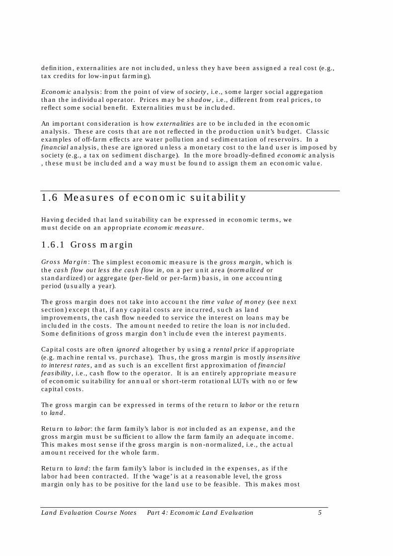
3.2 What is being optimized? the objective function
We want to maximize benefits to a production unit, i.e., the economic unit undera single manager, considered as a whole. In production agriculture, theproduction unit is usually the farm, which in turn is made up of managementunits, i.e., parcels that will be managed without further division. In forestry,the production unit is the set of parcels (lots) under single management, i.e., forwhich the benefits are aggregated by some manager.
In the simplest case, all the land on the farm is considered to be of the samequality, and land can be allocated to any use. This is a strong assumption sinceit doesn’t allow for different soil quality or permanent field boundaries. We willrelax this assumption later, but it simplifies the initial presentation.
In farm planning, we want to maximize the net return to the whole farm, forexample, the sum of the gross margins of all the land in the farm. The so-calledobjective function Z expresses the expected return:
Z R ai ii
= ⋅∑
where Ri is the net return per ha for land use i and ai is the area, in ha, to beallocated to use i.
Note: In project planning it may be more difficult to quantify the benefits. Itmay also be required to minimize the use of some resource, e.g. irrigationwater, rather than simply to maximize the return.
3.3 Constraints
There are four kinds of constraints to the allocation of land:
(1)The amount of land is limited: This is always a limitation: we can notallocate more land than we have. Furthermore, we must allocate non-negative amounts of land. This may be implicit in the model solution butusually must be explicitly stated, otherwise the solution may be unboundedor unphysical.

Land Evaluation Course Notes Part 4: Economic Land Evaluation 20
Sometimes land must be allocated in discrete amounts, e.g., in a watershedplan, if management unit boundaries are fixed and the operating authority isunwilling to split a unit among uses. Mathematically this is much moredifficult and may have no feasible solution. We will discuss this later.
(2) The amount of an input is limited: One or more production factors may bein limited supply. The most common limiting factors are labor hours andrelatively fixed assets such as machinery or animal power, and workingcapital. There may also be a limit on the amount of a variable input (suchas fertilizer) that can be obtained, but usually these are considered to beunlimited and their use is restricted by cost-benefit considerations.
Key point: these constraints on the amount of inputs may result in activitiesbeing included in the farm plan that are not the most profitable whenconsidered separately, because there are limitations on the resources thatwould be needed to allocate more area to these ‘better’ uses.
Example: a farm has only one drying floor for coffee beans, which can dry50kg of coffee every two days. The coffee can be picked for two months.Therefore the maximum amount of coffee that can be processed by this farmis 1,500kg. If the yield of coffee on this farm is 500kg ha-1, only 3 ha of coffeecan be grown no matter how profitable is the crop.
Example: a farm has only one tractor for plowing and sowing, which can work10 hours daily. To plow 1ha and prepare it for planting conventionally (disk,harrow etc.) requires 10h, to prepare with minimum tillage 2h. Five times asmuch land can be prepared with minimum tillage, as compared toconventional tillage. Even if the conventionally-tilled crop out-yields theminimum-tilled crop, or if the input costs are less for conventional tillage,since we only have one tractor, it may be that some land must be minimum-tilled only because of the shorter preparation time of this method.
Note in this example that the definition of the Land Utilization Type mustspecify the constraints, e.g., ‘with own machinery’. If there is the possibility ofcontracting an operator with machine (‘custom’ tillage), and there is nolimitation on the amount of time which can be contracted, this would be adifferent LUT: ‘with own machinery and contracting as necessary’; theconstraint would disappear and the cost of the contract would control whichland use to choose.
This is related to the ‘buy or rent’ problem. The farmer could borrow toincrease capital assets, e.g., in the first example, construct another dryingfloor. These are outside the scope of land evaluation; they are investmentdecisions.
(3) There are restrictions on the allocation of land: There may be policyreasons that require a minimum or maximum amount or proportion of land beallocated to a certain use. For example, in a forestry plantation of 10,000ha, it may be required that at least 1,000ha be allocated to high-qualitytrees for lumber, regardless of the economics, because of government ordonor policy. (It may turn out that more than 1,000ha will be allocated tohigh-quality trees.) Or in tourism development, it may be that at most 10%of the land can be developed, because otherwise the attractiveness of thearea for tourism would be diminished.
Land Evaluation Course Notes Part 4: Economic Land Evaluation 21
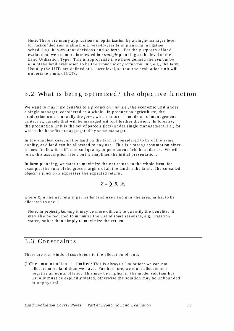
(4) There are restrictions on production: There may be policy reasons thatrequire that a minimum or maximum amount or proportion of product beproduced. For example, a farmer may have contracted to deliver at least 3Tof coffee; or, the farmer may only be allowed to deliver up to 3T of coffeebecause of a quota system to control production.
3.4 Mathematical programming
The techniques of mathematical programming are very well-developed (Hazell,1986, Hillier & Lieberman, 1986, Winston, 1991) and are appropriate fordetermining the optimum combination of land uses subject to constraints.Here the word ‘program’ refers (for historical reasons) to a set of equations, nota computer program.
The simplest kind of model is a linear model: all constraints must be linearcombinations, and the objective function also. This does not allow interactionsbetween constraints. There are fast methods to solve these programs.
If there are non-linear terms, the program is called non-linear (no duh!). If somevariables must be integers (e.g., whole machines), it is an integer program. Bothof these are harder to solve, but feasible for small programs.
3.5 Formulating the mathematical program
Reading: (Hazell, 1986) Chapters 2 and 3
The program will be formulated as a matrix: the columns are the ‘land utilizationtypes’ (activities) and the rows are the production factors.
1. Identify the land use options, also called the activities; these are the columnsof the model; the units of measure of the columns are land area, e.g.hectares.
2. Identify the independent variables (production factors such as labor,fertilizer, land, machinery); these are the rows of the model. The units ofmeasure of each row are specific to the input which the row represents. E.g.for labor it could be days, hours, weeks etc. For fertilizer it could be T, kg,bags etc.
3. Express the objective function, which is the sum of the returns from all theactivities, and whether it is to maximized (usual case) or minimized. Thereturns from activities are expressed on a per-land area basis (for example,$ ha
-1) and are computed for activity i as:
c yield price input pricei k k ik
l i ll
i
i
i
i
= ⋅ − ⋅∑ ∑

Land Evaluation Course Notes Part 4: Economic Land Evaluation 22
where the yields and input amounts are per-ha and the selling or buyingprices are per-unit of yield or input. The sums are over all ki outputs andall ji inputs for the activity. These net returns could be ALES gross margins,or they can be computed in a spreadsheet. In either case only theindividual activity returns c are entered in the matrix.
4. Express the constraints on the independent variables as a function of theactivities. These are the cells of the model; their units are in (units ofconstraint) (units of land area)
-1; i.e., the amount of the factor that is
necessary to implement the activity on a unit land area. The right hand sidegives the total amount of the constraint that is available to be allocated, in(units of constraint).
These are usually expressed in the linear programming tableau (why didn’t theyjust say ‘table’?). We follow the notation of (Hazell, 1986).
Activities X1 X2 ... Xn RHSObjectivefunction
c1 c2 ... cn Maximize
Resourceconstraints:1 a11 a12 ... a1n ≤ b12 a21 a22 ... a2n ≤ b2...
.
.
.
.
.
.
... ... ...
.
.
.
.
.
.m am1 am2 ... amn ≤ bn
Using this notation, we can write the ‘program’ as follows:
maxZ c Xj jj
n
==
∑1
(1)
such that
a X b i mij jj
n
i=
∑ ≤ ∀ =1
1� (2)
and
X j nj ≥ ∀ =0 1� (3)
Condition (1) is the objective function; we want maximum benefit from theactivities. Condition (2) are the set of n constraints on the activities. Condition(3) assures that all activities are positive.
Land Evaluation Course Notes Part 4: Economic Land Evaluation 23
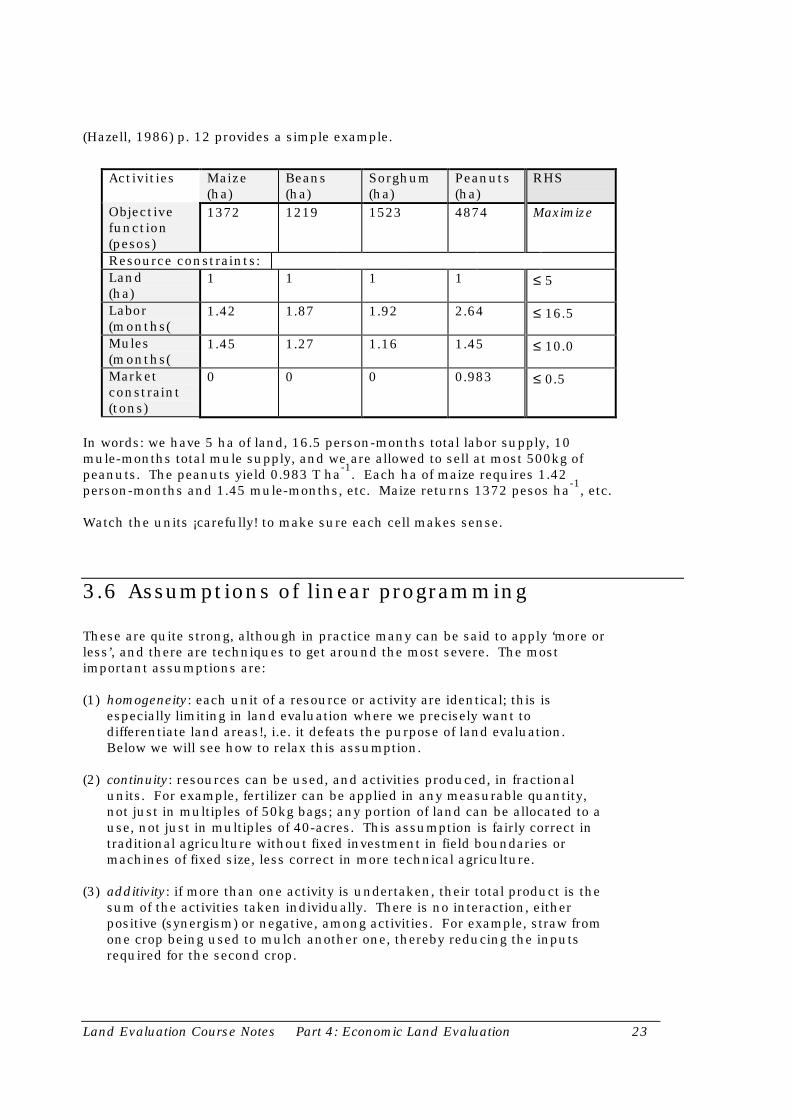
(Hazell, 1986) p. 12 provides a simple example.
Activities Maize(ha)
Beans(ha)
Sorghum(ha)
Peanuts(ha)
RHS
Objectivefunction(pesos)
1372 1219 1523 4874 Maximize
Resource constraints:Land(ha)
1 1 1 1 ≤ 5
Labor(months(
1.42 1.87 1.92 2.64 ≤ 16.5
Mules(months(
1.45 1.27 1.16 1.45 ≤ 10.0
Marketconstraint(tons)
0 0 0 0.983 ≤ 0.5
In words: we have 5 ha of land, 16.5 person-months total labor supply, 10mule-months total mule supply, and we are allowed to sell at most 500kg ofpeanuts. The peanuts yield 0.983 T ha
-1. Each ha of maize requires 1.42
person-months and 1.45 mule-months, etc. Maize returns 1372 pesos ha-1
, etc.
Watch the units ¡carefully! to make sure each cell makes sense.
3.6 Assumptions of linear programming
These are quite strong, although in practice many can be said to apply ‘more orless’, and there are techniques to get around the most severe. The mostimportant assumptions are:
(1) homogeneity: each unit of a resource or activity are identical; this isespecially limiting in land evaluation where we precisely want todifferentiate land areas!, i.e. it defeats the purpose of land evaluation.Below we will see how to relax this assumption.
(2) continuity: resources can be used, and activities produced, in fractionalunits. For example, fertilizer can be applied in any measurable quantity,not just in multiples of 50kg bags; any portion of land can be allocated to ause, not just in multiples of 40-acres. This assumption is fairly correct intraditional agriculture without fixed investment in field boundaries ormachines of fixed size, less correct in more technical agriculture.
(3) additivity: if more than one activity is undertaken, their total product is thesum of the activities taken individually. There is no interaction, eitherpositive (synergism) or negative, among activities. For example, straw fromone crop being used to mulch another one, thereby reducing the inputsrequired for the second crop.

Land Evaluation Course Notes Part 4: Economic Land Evaluation 24
(4) proportionality of returns: the gross margin is considered to be constant on aper-unit basis, i.e., there is no economy of scale nor diminishing returns.Among other things, this assumes perfect price elasticity, which isreasonable on a production unit that is only a small part of the totalproduction capacity.
(5) proportionality of production functions: the resource requirement isconsidered to be constant on a per-unit basis, i.e., there are no diminishingreturns as more of the input is used, nor is there any threshold effect. Allproduction functions are linear rays through the origin. For example, oneunit of fertilizer results in the same number of units of added production, nomatter how much fertilizer has been used. This is approximately true insome range where the production function is near-linear, oftencorresponding to realistic production scenarios.
In mathematical notation this assumption is:
kZ c kXj jj
n
==
∑ ( )1
(4)
so that by multiplying all production factors by k, the output is alsoincreased k times.
3.7 Solving the linear programming problem
A feasible solution, if one exists, is a set of activity levels that satisfy equations(1)-(3). The optimum solution, if one exists, is a feasible solution whose value ofthe objective function is equal to or better than that of any other feasiblesolution. Geometrically, the feasible solutions are the interior and boundarypoints of a convex region in the j-dimensioned space whose axes are defined bythe activities and whose boundaries are defined by the constraints. Theoptimum solutions are at one or more of the vertices of this region.
The most common computational method is the simplex method developed byDantzig in 1947 and since refined. It proceeds by allowing some activities intothe farm plan, and dropping others, until no further improvement can be made.In practice many less than the theoretical maximum number of combinationsare examined on the way to an optimum solution.
We will not present this or any other solution method; see (Hazell, 1986, Hillier& Lieberman, 1986, Winston, 1991) among many others for a detailedpresentation.
(The solution to the sample problem above is: 4.4914 ha sorghum and 0.5086ha peanuts, with 6.5338 months of labor and 4.0525 months of mules unused.The total gross margin is 9319.3 pesos.)
Various bad things can happen when trying to solve the problem:
(1) unfeasibility: there is no solution;

Land Evaluation Course Notes Part 4: Economic Land Evaluation 25
(2) unboundedness: the objective function can be increased without bound;
(3) degeneracy: as the simplex algorithm proceeds, it encounters ties amongincoming activities or activities that enter the solution at a zero level. Thereis a solution but the algorithm may not find it.
These problems usually occur because of incorrect model specification.
3.8 Slack variables
To solve inequality equations (e.g., total land use not to exceed 100ha, totallabor not to exceed 15 person-months), it is most convenient to convert theinequalities to equalities by introducing a so-called slack variable S:
a X b a X S bij jj
n
i ij jj
n
i i= =
∑ ∑≤ → + =1 1
(5)
In the solution to the linear program, the amount of slack indicates the amountof the resource that was not used and so was in oversupply. This is importantinformation for the planner. Slack values of zero (i.e., there was no slack, all ofthe resource was used) usually indicate that had more of the resource beenavailable, a different solution would have been obtained.
3.9 Duality and shadow prices
Equations (1) to (3) define the primal problem, which when solved tells theplanner how much of each activity to engage in, in order to maximize returns.To increase returns, the producer must acquire more of some fixed resource(the constraints), assuming that prices and yields don’t change. So... how muchshould the producer be willing to pay for another unit of some limitingresource? Below some price, it would be worthwhile because, having therebyrelaxed the constraint, a greater value of the objective function would beobtained.

Land Evaluation Course Notes Part 4: Economic Land Evaluation 26
In a linear programming problem, there is a single value of a limiting resourcethat answers these questions. It is known as the shadow price, or, in economictheory, the marginal value product. We can formulate the linear program so itdirectly supplies the shadow prices λi:
minW bi ii
m
==∑ λ
1
(1’)
such that
a c j nij ii
m
iλ=∑ ≥ ∀ =
1
1� (2’)
and
λi i m≥ ∀ =0 1� (3’)
The shadow prices, which (3) must be non-negative, are assigned such that (1)the total value W of the entire resource base is minimized, subject to theconstraints (2) that the total value of resources used by an activity is at leastthe gross margin c earned by that activity (otherwise we would be losing moneyon that activity). So we can think of this as a conservative approach to resourceallocation: we allocate the minimum value of resource possible, as long as wemeet the gross margin.
It turns out that this problem is the dual of (i.e., symmetric to) the primalproblem, in the sense that the coefficients are the same, but the matrix istransposed (rows become columns and vice versa), and the maximizationbecomes a minimization. The activity levels are implicit in the dual and explicitin the primal, whereas the shadow prices are implicit in the primal and explicitin the dual. In practice, codes that solve linear programs give shadow prices aswell as activity levels, i.e., they solve both the primal and dual problems.
Here is the general tableau for the dual problem:
Marginalvalues
λ1 λ2 ... λm RHS
Objectivefunction
b1 b2 ... bm Minimize
Activities:1 a11 a12 ... a1m ≥ c12 a21 a22 ... a2m ≥ c2...
.
.
.
.
.
.
... ... ...
.
.
.
.
.
.n an1 an2 ... anm ≥ cn
Here is the dual problem of the sample optimization problem. Notice that itcontains the same numbers, but the matrix is transposed, and the sense of the

Land Evaluation Course Notes Part 4: Economic Land Evaluation 27
inequalities has been reversed. Again, thinking about the units may make thisclearer.
Here is the dual of the example Mayaland tableau:
Marginalvalues
Land(pesos/ha)
Labor(pesos/month)
Mules(pesos.month)
Market(pesos/ton)
RHS
Objectivefunction(pesos)
5.0 16.5 10.0 0.5 Minimize
Activities:Maize (ha) 1 1.42 1.45 0 ≥ 1372Beans (ha) 1 1.87 1.27 0 ≥ 1219Sorghum (ha) 1 1.92 1.16 0 ≥ 1523Peanuts (ha) 1 2.64 1.45 0.983 ≥ 4874
3.10 Sensitivity analysis
In the linear programming model, all the coefficients a, b, and c are assumed tobe known without error and to be rigid. It is rarely the case that technicalcoefficients a (e.g., amount of yield increase per unit fertilizer) are known towith high accuracy. Also, prices and yields, which combine to the c coefficients,are also notoriously difficult to predict. Finally, the supposedly rigid constraintlevels b may in fact be somewhat flexible. For example, we may have calculatedthat only a certain amount of family labor is available; however, if the returnswere high enough, perhaps the family would work extra hours.
In sensitivity analysis, the coefficients are systematically varied until activitylevels change. This measures the sensitivity of the solution to the coefficients.For example, the range of possible input and output prices can be examined tosee if the activities should change, and if so, at what price points. Theinteresting thing here is that, even if we are somewhat wrong about prices andfactor levels, and hence about the actual value of the objective function that willbe attained, within a certain range we will still choose the same activities at thesame levels.
In parametric programming, a constraint is systematically relaxed until newactivities enter the solution. Then the planner can see at what point theconstraints change the decision. For example, the number of labor hours couldbe systematically relaxed until a different activity enters the solution; if thispoint is close to the original number of labor hours, perhaps the assumptionson which the available labor hours were based should be re-examined.
These methods are easy (albeit computationally-intensive) once the model hasbeen built, and they provide extra information to the planner.

Land Evaluation Course Notes Part 4: Economic Land Evaluation 28
3.11 Modeling more realistic production scenarios
The assumptions of linear programming may seem rigid, but there are variousways to circumvent them in order to model realistic production scenarios.(Hazell, 1986) Ch. 3 has a good introduction to modeling a choice of productionmethods, factor substitution, non-linear input/output response, seasonality,quality difference in resources, buying and selling alternatives, crop rotations,inter-cropping and joint products, intermediate products, and credit/cash flowconstraints. We will examine the most important of these to land evaluation,i.e., quality differences in resources.
In land evaluation, the whole point is that different land areas vary in theirability to produce or in the amount of inputs necessary to do this. Thesedifferences are modeled in the linear program by replacing a single ‘land’resource with the different kinds of ‘land’, each with its area as the right-hand-side constraint, and with different coefficients in the objective function andconstraint equations. For example:
Maize on‘CeB’, ha
Maize on‘HnA’, ha
Wheat on‘CeB’, ha
Wheat on‘HnA’, ha
RHS
Objectivefunction
120bu ∗$2 bu
-1
- 80 kg ∗$1 kg
-1
100bu ∗$2 bu
-1
- 60 kg ∗$1 kg
-1
50 bu ∗$1.50 bu
-1
- 40 kg ∗$1 kg
-1
60 bu ∗$1.50 bu
-1
- 30 kg ∗$1 kg
-1
Maximize
Resource constraints:Soil ‘CeB’, ha 1 0 1 0 ≤ 20 haSoil ‘HnA’, ha 0 1 0 1 ≤ 40 ha
There are separate yields (part of the c’s, to be multiplied by the price, which isthe same no matter what land is used) and the production factors for soils ‘CeB’and ‘HnA’. You can see that the number of hectares of each soil type are limitedby the amount of that type which is available. Also they are fertilizeddifferently, which affects the gross margins (the total amount of fertilizer is not alimiting factor).
The solution to this problem may divide a soil unit among different uses. Landcan be allocated in any amount, not just in whole hectares.
3.12 Using the results of ALES evaluations in linearprograms
ALES can predict net returns (gross margin or NPV) on a per-land-unit basis(non-normalized) for each land unit/land use combination, without taking intoaccount constraints. The per-hectare unit values are multiplied by the size ofthe evaluation unit by the program, as long as land areas have been enteredinto the database for each map unit. If the map units are defined asmanagement units (e.g., fields) we have the predicted return of each decision unit

Land Evaluation Course Notes Part 4: Economic Land Evaluation 29
for each possible use, otherwise the predicted return for some ‘natural’delineations. The gross margins go directly into the objective function.
(ALES can also produce normalized or per-unit-area results. If areas of the farmcan be allocated in fractional units, i.e., existing field boundaries are notimportant, this is the appropriate measure. In this case, the ‘natural’ units(such as soils) are the ALES map units.)
Example of an evaluation results matrix:
net return, $ LUT1 LUT2 LUT3ManagementUnit1 1100 200 0ManagementUnit2 200 1000 2000ManagementUnit3 0 100 500
The ALES matrix can be exported to a spreadsheet with an optimizer (e.g., MSExcel, Quattro Pro) or to a specialized linear program model.
The technical coefficients (i.e., amount of each input needed to produce 1 ha ofan activity) may also be exported to a spreadsheet, to be used in the LP:
hrs of labor LUT1 LUT2 LUT3ManagementUnit1 20 20 10ManagementUnit2 30 20 10ManagementUnit3 10 30 20

Land Evaluation Course Notes Part 4: Economic Land Evaluation 30
4. Risk analysis
Bibliography: in farm planning: (Hazell, 1986) Ch. 5; in a policy-analysisframework: (Morgan & Henrion, 1990); in the context of GIS, “The DecisionSupport Ring” (pp. 35-61) in (Eastman, 1993).
Software: @RISK (Palisade Corp., Newfield NY) add-in for MS Excel and Lotus 1-2-3.
In the previous lecture we showed how linear programming can be used tooptimize under constraints. However, consider the following uncertainties in thelinear programming tableau:
(1)The response of the land use to production factors. These affect thetechnical coefficients.
(2)The actual value of static land data for each map unit in the plan. Theseaffect the technical coefficients and the objective function. For example,levels of soil nutrients.
Furthermore, consider the uncertainty about the future state of nature, i.e.,what the future will hold. These are usually called risks because they areunknowable at present:
(1)Prices. In market economies these are subject to change. They affect theobjective function.
(2)The availability of production factors. These affect the right-hand side, i.e.constraints.
(3)The weather. This usually has a tremendous impact on production, andhence the objective function. Since the weather is an important time series,this uncertainty leads to a time series of results. One famous case is the‘Tanganyika groundnut (peanut) scheme’ of the early 1950’s. The expectedcase was favorable but the time series of outcomes was not, because therewere too many consecutive years with low returns.
So a static analysis using expected values for factors that are known to bevariable is only satisfactory for the expected or average case. It provides noinformation on the expected range of results. This information is provided byrisk analysis, perhaps better called uncertainty analysis.
The basic idea is that a land evaluation should provide information on the rangeand likelihood of all possible outcomes. Then, the risk-taking behavior of theplanner can be explicitly included in the process.
We considered some of these same issues in the ‘sensitivity analysis’ section ofthe previous lecture. In that section, we examine ways in which the analyst can
Land Evaluation Course Notes Part 4: Economic Land Evaluation 31
determine how sensitive the solution is to uncertainty. Here the emphasis is onhow much risk is inherent in a certain decision.
4.1 Uncertainty, risk, & risk-taking behavior
Uncertainty is doubt about phenomena that we have already observed,expressed in probabilistic form. ‘Uncertainty’ in this sense means that we arenot sure of what we actually observed (typically because of experimental andobservational error). We can reduce uncertainty with more experimentation,but it will not be cost-effective to do this past a certain point. In the linearprogram, ‘uncertainty’ usually refers to technical coefficients .
In an economic model, uncertainty usually refers to the technical coefficients ofthe model, based on experiment, observation, and expert knowledge. Forexample, how many labor hours does it take to grow a hectare of maize? It mayalso refer natural resource data, which affects the objective function. Forexample, how much water-holding capacity does this soil have?
Risk is doubt about unknowable phenomena, expressed in probabilistic form.‘Unknowable’ in this sense usually means that we are predicting the future, andthe outcomes may not be what we expect or what we have observed over time inthe past. No amount of observation can predict the future, although long time-series of historical data will help us infer what the future may hold.
Eastman (1993) phrases this a bit differently: “Risk may be understood as thelikelihood that the decision made will be wrong”. (p. 40); in addition we maytake into account the cost of the wrong decision.
In an economic model, risk refers to the so-called states of nature, i.e., what willhappen in the future with factors beyond our control such as weather andmarkets. States of nature can also refer to alternative states of our knowledgeabout technical coefficients, even though these do not depend on future events;this is a less common use of the term.
Risk-taking behavior is the attitude of someone (in our case, a decision maker)to risk. Below we will see various ways to quantify this. Most people are riskaverse, i.e., they are willing to trade some income for a more certain time seriesof incomes.
In land evaluation, we should take the risk aversion of the land users intoaccount when comparing land use alternatives, since some land uses may bemore risky than others, even if their expected value over time is the same. Thefactor ‘risk aversion of land users’ becomes part of the definition of the LandUtilization Type, and then part of the decision procedure.

Land Evaluation Course Notes Part 4: Economic Land Evaluation 32
4.2 Payoff matrix, expected value, and variance
In order to quantify risk-taking behavior, we first need some more definitions.
Payoff matrix
The outcomes for each state of nature are assigned probabilities of occurrence;each outcome also has a value (e.g., a gross margin). From this we formulatethe payoff matrix:
State ofnature
S1 S2 ... St
LUT1 Y11
Y12 ... Y1t
LUT2 Y21
Y22 ... Y2t
... ... ... ... ...LUTj Yj1 Yj2 ... Yjt
probability p1 p2 ... pt
The states of nature Sj are the possible scenarios, e.g., combinations of weatherand prices. The Yij’s are the gross margins to be realized for a given LUTi if agiven state of nature Sj occurs. Note that this matrix only expresses risk in thestates of nature, not the uncertainty in the technical coefficients of the farmmodel.
Of course, the tricky part is assigning the probabilities. In the case of historicaltime-series, we simply assign each member of the time series its proportionaloccurrence, for example, in a ten-year time series, each year has a probability of0.10. Another approach is to take percentiles of a known or assumedprobability distribution, according to the resolution we need. For example, a10-column payoff matrix, with the values from the midpoints of the deciles of anormal distribution.
Expected value
Once the probability of each state of nature is assigned, we can compute theexpected value for the LUT over all states of nature as the weighted (by theprobability) sum of the outcomes for the LUT.
E Y Y pi ii t
[ ] ==∑1�
Variance
Many measures of risk use the variance of the value of the LUT over time. Thiscan also be computed from the payoff matrix:
V Y p Y Yj ii t
[ ] ( )= −=∑ 2
1�

Land Evaluation Course Notes Part 4: Economic Land Evaluation 33
4.3 Expressing risk aversion
If we had unlimited reserves or means to get us through low-income years, wewould prefer the greatest expected value. However, in practice we are willing totrade some total income (over a long period) for ‘smoother’ and ‘more certain’incomes in the short and medium term. The degree to which we are willing toforego overall benefit for more certainty (i.e., lower expected value for lowervariance) is measured by our risk aversion.
From first principles of how an individual ‘should’ perceive and evaluate risk,we can derive a utility function U(Y) which expresses the ‘goodness’, in terms ofthe individual’s preference, for a LUT Y. One possibility is the expected value;in this case the individual is risk-neutral and can stand indefinite runs ofunfavorable states of nature in anticipation of sufficient benefits in favorablestates of nature. Usually the individual has some risk aversion, so somethingother than just expected value must be included in the utility function. Mostcommonly this is the variance as defined above.
Note that we are now using the general concept of utility to evaluatealternatives. The expected net income is only one measure of utility. A moregeneral measure of utility should incorporate both expected value and variance.
There are several possible utility functions, which satisfy a set of axioms, suchas self-consistency. We then choose among utility functions according to howwell they model human risk-taking behavior. A common utility function is thequadratic utility function:
U Y Y Y( ) = ⋅ + ⋅α β 2
where α and β are constants that are determined experimentally for eachindividual, using carefully-designed games. The idea here is that α is thedegree to which the expected return is valued (linear) whereas β weights thevariance. We can see this by taking the expected value of the utility function:
E[U(Y)] = αE[Y] + βE[Y²]= αE[Y] + βE[Y²] - (βE[Y]² + βE[Y]²), now group the two middle terms:= αE[Y] + βE[Y]² + βV[Y]
If α>0 and β < 0, the farmer will prefer higher expected incomes E[Y] and lowervariances of income V[Y]. If E[Y] for several LUTs are the same, the LUT withthe lower variance V[Y] will be preferred, because since β < 0, the higher thevariance the lower the utility.
We now examine three ways to evaluate risk: (1) (E,V) analysis, (2) MOTAD, and(3) Safety-first.
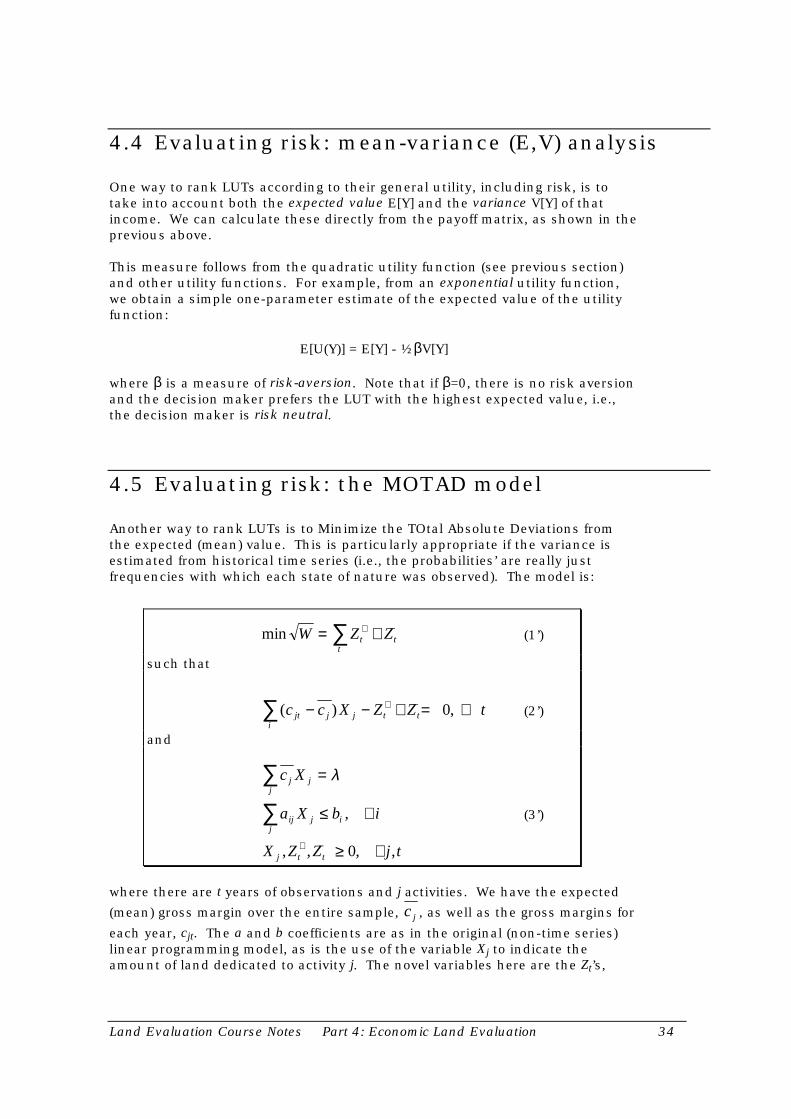
Land Evaluation Course Notes Part 4: Economic Land Evaluation 34
4.4 Evaluating risk: mean-variance (E,V) analysis
One way to rank LUTs according to their general utility, including risk, is totake into account both the expected value E[Y] and the variance V[Y] of thatincome. We can calculate these directly from the payoff matrix, as shown in theprevious above.
This measure follows from the quadratic utility function (see previous section)and other utility functions. For example, from an exponential utility function,we obtain a simple one-parameter estimate of the expected value of the utilityfunction:
E[U(Y)] = E[Y] - ½βV[Y]
where β is a measure of risk-aversion. Note that if β=0, there is no risk aversionand the decision maker prefers the LUT with the highest expected value, i.e.,the decision maker is risk neutral.
4.5 Evaluating risk: the MOTAD model
Another way to rank LUTs is to Minimize the TOtal Absolute Deviations fromthe expected (mean) value. This is particularly appropriate if the variance isestimated from historical time series (i.e., the probabilities’ are really justfrequencies with which each state of nature was observed). The model is:
min W Z Zt tt
= ++ −∑ (1’)
such that
( ) ,c c X Z Z tjt ji
j t t− − + = ∀∑ + − 0 (2’)
and
c X
a X b i
X Z Z j t
j jj
ij j ij
j t t
=
≤ ∀
≥ ∀
∑∑
+ −
λ
,
, , , ,0
(3’)
where there are t years of observations and j activities. We have the expected
(mean) gross margin over the entire sample, cj , as well as the gross margins for
each year, cjt. The a and b coefficients are as in the original (non-time series)linear programming model, as is the use of the variable Xj to indicate theamount of land dedicated to activity j. The novel variables here are the Zt’s,

Land Evaluation Course Notes Part 4: Economic Land Evaluation 35
which measure the positive (Z+) or negative (Z- ) deviations of the return for the
farm plan in year t from the mean value.
4.6 Evaluating risk: safety-first
Many resource-poor farmers can not even afford one year that is too severe. Ifthey can not meet their food and credit obligations, they will be obliged to sell,move, or even face starvation. A class of models that are designed to rank farmplans by maximizing their minimum levels over some sequence of state of natureare known as safety-first models.
Roy, in 1952, suggested selecting the farm plan that minimizes Pr{Yt ≤ Y0},where Y0 is the minimum acceptable income. There are problems actuallycomputing this efficiently. Another way to view this problem is to select a farmplan that always (i.e., in every state of nature) returns at least the ‘safety-first’level Y0 and otherwise maximizes expected income. This is Low’s safety-firstmodel:
maxE c Xj jj
n
==
∑1
(1)
such that
a X b i mij jj
n
i=
∑ ≤ ∀ =1
1� (2)
and
X j nj ≥ ∀ =0 1� (3)
and the ‘safety-first’ criterion:
c X Y t kjtj
n
j=
∑ ≥ ∀ =1
0 1� (3)
This can be solved with standard LP algorithms. The problem is that there maynot be a feasible solution if the safety-first goal is too large relative to E or if therisks are inherently too high (i.e., the cjt’s are too variable). Actually, the non-existence of a solution suggests that either (1) the farmer has unrealistically-high expectations for the worst-case and should look into ways to raise thevalue of the minimum acceptable Y0 , or, (2) there is no acceptable plan giventhe current risk environment. This is valuable information to planners: it wouldseem to indicate the need for crop or disaster insurance, or some other ‘safetynet’ program, to raise the level of the minimum acceptable worst-case.

Land Evaluation Course Notes Part 4: Economic Land Evaluation 36
4.7 The @RISK software
The @RISK software provides a fast, flexible and graphical way to examine theeffects of uncertainty. It takes a ‘Monte Carlo’ simulation approach. The basicprocedure is as follows:
1. The analyst (e.g., land evaluator) builds a spreadsheet to express theeconomic results of the evaluation; this may be a linear program to besolved.
2. The analyst specifies probability or frequency distributions for one or moreinput cells in the spreadsheet model. For example, prices could have anormal distribution with a specified mean and variance. Climate could havea lognormal or Weibull distribution. Or, specific states of nature can beentered as a discrete distribution. This applies to uncertainty (e.g., intechnical coefficients) as well as to future states of nature.
3. At the command of the analyst, @RISK generates samples from eachdistribution to create scenarios, which are possible combinations of allvariables. Then the host spreadsheet (e.g., MS Excel) re-computes thespreadsheet. @RISK collects statistics for result cells specified by theanalyst. These might be activity mix or profitability.
4. Step (3) is repeated many times, usually 1000’s.
5. @RISK displays a frequency distribution and statistics for the result cells.These can be used in safety-first models (e.g., find the highest-payoff planthat satisfies Roy’s criterion) or in (E,V) analysis (because the empiricalresult distribution provides an estimate of the mean and variance of theoutcome).
The hardest part of using @RISK, or any Monte Carlo method, is obtainingreliable information about the probability or frequency distributions.

Land Evaluation Course Notes Part 4: Economic Land Evaluation 37
5. Decision theory and multi-objectivedecision making
The aim of this lecture is to place decision-making into a theoretical framework,and to classify decision procedures. It draws heavily from the article “TheDecision Support Ring” (pp. 35-61) in (Eastman, 1993).
5.1 Definitions
Decision: a choice between alternatives
Criterion: some basis for a decision; of two types: factors and constraints
- Factor: enhances or detracts from the suitability of a land use alternative on amore-or-less continuous (or at least ordinal) scale, e.g., higher water-holding capacity is generally a positive factor for rainfed agriculture
- Constraint: limits the alternatives. We have seen this in the discussion ofeconomic optimization. This is often used to mean ‘negative constraint’,e.g., only 10ha of land are available.
- Goal or Target: some characteristic that the solution must possess, a ‘positiveconstraint’, e.g., at least 5T of peanuts must be produced to satisfy acontract. This was also considered a ‘constraint’ in economic optimization,but we can see that it has a fundamentally-different character: it refers to aconstraint on the solution, not on the problem.
Decision rule: the procedure by which criteria are combined to make adecision. Typically the criteria are combined into a single ordinal index, bywhich alternatives can be ranked. Example: gross margins of all thealternatives which satisfy the constraints; the linear program wouldautomatically find the most profitable decision. Another example: thealternative that gives the ‘best’ combination of expected return and itsvariance, i.e., the best utility given a certain formulation of risk.
A decision tree is an example of a decision rule.
Eastman divides decision rules into choice functions (numerical, exact) andchoice heuristics (approximate procedures for finding a solution that is ‘goodenough’).
Objective: the measure by which the decision rule operates. E.g., maximizeincome, maximize utility, minimize pollution.

Land Evaluation Course Notes Part 4: Economic Land Evaluation 38
Evaluation: the actual process of applying the decision rule. Note this is amore general sense of the word that as it is used in ‘land evaluation’.
5.2 Kinds of evaluations
We can consider evaluations on two axes: (1) number of criteria and (2) numberof objectives.
Single-criterion evaluation: only one criterion is necessary to evaluate. Fairlyrare, but sometimes one criterion is over-riding.
Multi-criteria evaluations: to meet one objective, almost always several criteriawill have to be combined.
Multi-objective evaluations: very often we have several objectives at the sametime. These can be divided into two groups, depending on the relationbetween objectives:
- Complementary objectives: non-conflicting, in land evaluation terms, thesame area of land can satisfy several complementary objectives at the sametime (e.g., extensive grazing and recreational hiking). To this point, we haveincluded both complementary objectives in a single LUT and evaluated forboth at the same time.
- Conflicting objectives: land can be used for one use or the other, but notboth. This is the way we have been viewing competing LUTs in landevaluation, to this point.
We can organize decision-making processes in a 3x2 matrix:
Single criterion Multi-criteria
Single-objective
Multi-objective,complementary
Multi-objective,conflicting
The single-criterion, single-objective case is not very interesting. In landevaluation terms, it corresponds to the case where a LUT is defined by only oneLUR. An example might be: LUT ‘biodiversity reserve’, one LUR: ‘existence ofprimary forest’, one LC (same), a simple decision rule: ‘All areas in primaryforest go to the biodiversity reserve, all others stay out’. The problems with thisanalysis should be evident.
We have been working at the single-objective, multi-criteria case. In the previousexample, we would also rate things like LUR ‘distance from population

Land Evaluation Course Notes Part 4: Economic Land Evaluation 39
pressure’, ‘adequate contiguous area’, ‘not highly-suited to valuable hardwoodspecies’, etc.
The multiple-objective, single-criterion case is also unlikely. This would be withseveral conflicting LUTs, all evaluated with the same single LUR.
The multiple-objective, multiple-criterion case is the most realistic and interesting.Especially important are when the multiple objectives come from different users(consumers, decision makers). For example, conservationists may have theobjective of a certain area of high-quality biodiversity reserve, whereas afarmer’s cooperative may have the objective of maximizing income from high-value highland crops, whereas a local water authority may have the objective ofassuring a reliable source of pure water for municipal supply.
5.3 Multi-criteria decision making
A simple formulation of a decision rule for continuous criteria is the weightedlinear combination:
S w xi ii
= ∑
where S is the composite suitability score, based on individual scores x andtheir weights w, which usually sum to 1. If Boolean (yes/no) factors are alsoincluded, these multiply the suitability score, to eliminate those without all‘true’ scores for the Boolean factors c:
S w x ci ii
jj
= ×∑ ∏
IDRISI provides the module MCE to combine a group of factor maps. The bigproblem, however, is: How are the factor weights established?
In the original FAO method, factors (LQs) are combined by a maximum-limitation method, so all weights are equal. In ALES, arbitrary decision treescan be used. For continuous factors to be combined by GIS, the variouscriterion scores must be standardized: all factors must be on the same scale andpositively correlated with suitability (this may require the inversion of somemaps).
5.3.1 Standardizing criteria to a common scale
To standardize to the same scale, we can apply a simple linear stretch (e.g.,IDRISI module STRETCH, the same that is applied to images):
x r r r r new rangei i= − − ⋅( ) / ( ) _min max min
where r are the raw scores in the original units of measure and new_range isthe range to which all factors will be standardized.

Land Evaluation Course Notes Part 4: Economic Land Evaluation 40
5.3.2 Assigning criterion weights
Much trickier is how to weight the criterion. This is often a subjective decision.For example, how much more important is ‘gentle slope’, compared to ‘bedrockgeology’, when deciding where to site a new industry? (If we can assigneconomic costs to each of these, as in ALES’s ‘reduced yields’ or ‘increased coststo compensate’, the issue of weighting goes away.) Psychological tests can beused to rank and compare criteria. A technique devised by Saaty (1977)compares each factor in pairs until a self-consistent set of weights is found.The expert assigns an importance to each criterion, on the following scale:
extremely
very strongly moderately
equally moderately
strongly very extremely
1/9 1/7 1/5 1/3 1 3 5 7 9less important more
important
So, a matrix is created (actually, only one half of the symmetric matrix must befilled in) containing n²/2-n comparisons (the diagonals are always 1, i.e., afactor is equal in importance to itself).
Taking the principal components of this matrix gives the principal eigenvector ofthe matrix, which is exactly the best estimate of the factor ratings to be used inthe multi-criteria evaluation. The weights will sum to 1. At the same time, theother eigenvectors can indicate how consistent are the pairwise comparisonsgiven by the expert.
Now with the criteria on a common scale, and weighted, we can compute overallsuitability with MCE.
5.4 Multi-objective decision making
The interesting case here is when there are conflicting objectives.
5.4.1 Prioritizing objectives
One easy solution is to prioritize objectives. Then we evaluate for the firstobjective, and allocate land as necessary to meet that objective. The allocatedland is removed from consideration, and we then evaluate for the secondobjective, and allocate land as necessary for this objective. Note that thissecond step may not be possible, because some very desirable land for thesecond objective may have been already allocated for the first objective.
IDRISI V4.1 provides the RANK module to rank all the cells in an imageaccording to their suitability scores. HISTO can be used to examine thefrequency distribution of the ranks. Then RECLASS can be used to allocate therequired proportion of cells to the first objective.

Land Evaluation Course Notes Part 4: Economic Land Evaluation 41
5.4.2 Compromise solutions
If there is no clear prioritization, as is usually the case, we must seek acompromise solution. In an economic land evaluation context, it may be possibleto formulate a linear program (optimization under constraints). However thisprogram may not have a solution, i.e., there is no one perfect solution; insteadsome compromises must be made.
IDRISI V4.1 includes the MOLA (multi-objective land allocation) module toassign land under compromises. We can visualize its operation with twoconflicting objectives:
The conflicting region is where both objectives are highly-suitable (i.e., pasttheir respective thresholds for ‘highly suitable’).’
5.4.3 Standardizing scores for multiple objectives
Before a conflict-resolution procedure such as MOLA can be run, the suitabilityscores for each objective must be standardized, i.e., put on the same scale of‘goodness’. This can be accomplished by STRETCH (‘histogram equalization’option) or STANDARD if the distribution is approximately normal.
5.4.4 Use of secondary criteria to break ties
All other things being equal, we would prefer to allocate cells in reverse order ofsuitability for a conflicting objective. MOLA can do this if we provide it asecondary image, which contains this information.

Land Evaluation Course Notes Part 4: Economic Land Evaluation 42
6. References
1. Barlowe, R. 1986. Land resource economics: the economics of real estate. 4thed. Englewood Cliffs, NJ: Prentice-Hall. 559 pp. HD.111 B25 1986 Mann
2. Carlson, G.A., Zilberman, D. & Miranowski, J.A. 1993. Agricultural andenvironmental resource economics. New York: Oxford University Press. ix, 528pp. HD 1433 A353x 1993 Mann
3. Colman, D. & Young, T. 1989. Principles of agricultural economics: marketsand prices in less developed countries. Wye Studies in Agricultural and RuralDevelopment, Cambridge: Cambridge University Press. 323 pp. HD1417.C71 1989 Mann
4. Dent, D. & Young, A. 1981. Soil survey and land evaluation. London,England: George Allen & Unwin. S592 .14.D41 Mann
5. Dovring, F. 1987. Land economics. Boston: Breton Publishers. xi, 532 pp. HD111 D74 1987 Mann
6. Eastman, J.R. 1992a. IDRISI Version 4.0 Technical Reference. Worcester, MA:Clark University Graduate School of Geography. 213 pp.
7. Eastman, J.R. 1992b. IDRISI Version 4.0 User's Guide. Worcester, MA: ClarkUniversity Graduate School of Geography. 178 pp.
8. Eastman, J.R. 1993. IDRISI Version 4.1 Update Manual. Worcester, MA: ClarkUniversity Graduate School of Geography. 211 pp.
9. EUROCONSULT. 1989. Agricultural Compendium for rural development in thetropics and subtropics. Amsterdam: Elsevier. 740 pp. S481 .A27 1989 Mann
10. Ghatak, S. & Ingersent, K. 1984. Agriculture and economic development.The Johns Hopkins Series in Development, Baltimore: Johns HopkinsUniversity Press. xii, 380 pp. HD1417 .G41 1984
11. Hazell, P.B.R. 1986. Mathematical programming for economic analysis inagriculture. New York: Macmillan. 400 pp. HD1433.H42 1986 Mann, MannReserve
12. Hillier, F.S. & Lieberman, G.J. 1986. Introduction to operations research.4th ed. Oakland, CA: Holden-Day. xviii, 888 pp. Q175 .H65 1986 Carpenter
13. Johnson, A.K.L. & Cramb, R.A. 1991. Development of a simulation basedland evaluation system using crop modelling, expert systems and risk analysis.Soil Use Manag. 7(4): 239-245.
14. Johnson, A.K.L. & Cramb, R.A. 1992. An integrated approach toagricultural land evaluation: Report to the Land & Water Resources Research

Land Evaluation Course Notes Part 4: Economic Land Evaluation 43
and Development Corporation on developing alternative procedures in landevaluation. Vol. 5; Results of a case study in the Herbert River District ofnorth Queensland. Queensland, Australia: Department of Agriculture, theUniversity of Queensland.
15. León Pérez, J.C. 1992. Aplicación del sistema automatizado para laevaluación de tierras-ALES, en un sector de la cuenca del río Sinú (Córdoba-Colombia). Revista CIAF 13(1): 19-42.
16. Morgan, M.G. & Henrion, M. 1990. Uncertainty : a guide to dealing withuncertainty in quantitative risk and policy analysis. New York: CambridgeUniversity Press. x, 332 pp. pp. HB615 .M665x 1990 Olin
17. Newman, D.G. 1991. Engineering economic analysis. 4th ed. San Jose,CA: Engineering Press. 578 pp.
18. Riquier, J. 1974. A summary of parametric methods of soil and landevaluation, in Approaches to land classification, Soils Bulletin 22, FAO, Editor.Rome: FAO.
19. Saaty, T.L. 1977. A scaling method for priorities in hierarchical structures.J. Math. Psychology 15: 234-281.
20. Storie, R.E. 1933. An index for rating the agricultural value of soils.Bulletin - California Agricultural Experiment Station, Vol. 556. Berkley, CA:University of California Agricultural Experiment Station. S39. E21 Mann
21. U.S. Department of the Interior, B.o.R. 1951. Irrigated land use, Part 2:Land classification. Bureau of Reclamation Manual, Vol. 5. Washington: U.S.Government Printing Office.
22. Winston, W.L. 1991. Operations research: applications and algorithms.2nd ed. Boston: PWS-Kent. 1262 pp. T57.6 .W78 1991 Engineering reserve
23. Young, A. & Goldsmith, P.F. 1977. Soil survey and land evaluation indeveloping countries: a case study in Malawi. Geogr. J. 143: 407-431.