Embed Size (px)
Citation preview

Lecture Notes in Mathematics 1982
Editors:J.-M. Morel, CachanF. Takens, GroningenB. Teissier, Paris
Nicolas Privault
Stochastic Analysisin Discrete andContinuous Settings
With Normal Martingales
123
Nicolas PrivaultDepartment of MathematicsCity University of Hong KongTat Chee AvenueKowloon TongHong KongP.R. [email protected]
ISBN: 978-3-642-02379-8 e-ISBN: 978-3-642-02380-4DOI: 10.1007/978-3-642-02380-4
Lecture Notes in Mathematics ISSN print edition: 0075-8434ISSN electronic edition: 1617-9692
Library of Congress Control Number: 2009929703
Mathematics Subject Classification (2000): 60H07, 60G44, 60G42, 60J65, 60J75, 91B28
c© Springer-Verlag Berlin Heidelberg 2009This work is subject to copyright. All rights are reserved, whether the whole or part of the material isconcerned, specifically the rights of translation, reprinting, reuse of illustrations, recitation, broadcasting,reproduction on microfilm or in any other way, and storage in data banks. Duplication of this publicationor parts thereof is permitted only under the provisions of the German Copyright Law of September 9,1965, in its current version, and permission for use must always be obtained from Springer. Violationsare liable to prosecution under the German Copyright Law.
The use of general descriptive names, registered names, trademarks, etc. in this publication does notimply, even in the absence of a specific statement, that such names are exempt from the relevant protectivelaws and regulations and therefore free for general use.
Cover design: SPi Publisher Services
Printed on acid-free paper
springer.com
Preface
This monograph is an introduction to some aspects of stochastic analysis inthe framework of normal martingales, in both discrete and continuous time.The text is mostly self-contained, except for Section 5.7 that requires somebackground in geometry, and should be accessible to graduate students andresearchers having already received a basic training in probability. Prerequi-sites are mostly limited to a knowledge of measure theory and probability,namely σ-algebras, expectations, and conditional expectations. A short intro-duction to stochastic calculus for continuous and jump processes is given inChapter 2 using normal martingales, whose predictable quadratic variationis the Lebesgue measure.
There already exists several books devoted to stochastic analysis for con-tinuous diffusion processes on Gaussian and Wiener spaces, cf. e.g. [51], [63],[65], [72], [83], [84], [92], [128], [134], [143], [146], [147]. The particular fea-ture of this text is to simultaneously consider continuous processes and jumpprocesses in the unified framework of normal martingales.
These notes have grown from several versions of graduate courses givenin the Master in Imaging and Computation at the University of La Rochelleand in the Master of Mathematics and Applications at the University ofPoitiers, as well as from lectures presented at the universities of Ankara,Greifswald, Marne la Vallee, Tunis, and Wuhan, at the invitations ofG. Wallet, M. Arnaudon, H. Korezlioglu, U. Franz, A. Sulem, H. Ouerdiane,and L.M. Wu, respectively. The text has also benefited from constructiveremarks from several colleagues and former students, including D. David,A. Joulin, Y.T. Ma, C. Pintoux, and A. Reveillac. I thank in particularJ.C. Breton for numerous suggestions and corrections.
Hong Kong, Nicolas PrivaultMay 2009
v

Contents
Introduction . . . . . . . . . . . . . . . . . . . . . . . . . . . . . . . . . . . . . . . . . . . . . . . . . . . . . . . . . . . . . . . . 1
1 The Discrete Time Case . . . . . . . . . . . . . . . . . . . . . . . . . . . . . . . . . . . . . . . . . . . . . 71.1 Normal Martingales . . . . . . . . . . . . . . . . . . . . . . . . . . . . . . . . . . . . . . . . . . . . . . . . 71.2 Stochastic Integrals . . . . . . . . . . . . . . . . . . . . . . . . . . . . . . . . . . . . . . . . . . . . . . . . 81.3 Multiple Stochastic Integrals . . . . . . . . . . . . . . . . . . . . . . . . . . . . . . . . . . . . . . 111.4 Structure Equations .. . . . . . . . . . . . . . . . . . . . . . . . . . . . . . . . . . . . . . . . . . . . . . . 131.5 Chaos Representation .. . . . . . . . . . . . . . . . . . . . . . . . . . . . . . . . . . . . . . . . . . . . . 151.6 Gradient Operator . . . . . . . . . . . . . . . . . . . . . . . . . . . . . . . . . . . . . . . . . . . . . . . . . 181.7 Clark Formula and Predictable Representation .. . . . . . . . . . . . . . . . . 221.8 Divergence Operator . . . . . . . . . . . . . . . . . . . . . . . . . . . . . . . . . . . . . . . . . . . . . . . 241.9 Ornstein-Uhlenbeck Semi-Group and Process . . . . . . . . . . . . . . . . . . . . 281.10 Covariance Identities . . . . . . . . . . . . . . . . . . . . . . . . . . . . . . . . . . . . . . . . . . . . . . . 321.11 Deviation Inequalities . . . . . . . . . . . . . . . . . . . . . . . . . . . . . . . . . . . . . . . . . . . . . . 361.12 Logarithmic Sobolev Inequalities. . . . . . . . . . . . . . . . . . . . . . . . . . . . . . . . . . 421.13 Change of Variable Formula .. . . . . . . . . . . . . . . . . . . . . . . . . . . . . . . . . . . . . . 491.14 Option Hedging. . . . . . . . . . . . . . . . . . . . . . . . . . . . . . . . . . . . . . . . . . . . . . . . . . . . . 531.15 Notes and References . . . . . . . . . . . . . . . . . . . . . . . . . . . . . . . . . . . . . . . . . . . . . . 58
2 Continuous Time Normal Martingales . . . . . . . . . . . . . . . . . . . . . . . . . . . 592.1 Normal Martingales . . . . . . . . . . . . . . . . . . . . . . . . . . . . . . . . . . . . . . . . . . . . . . . . 592.2 Brownian Motion . . . . . . . . . . . . . . . . . . . . . . . . . . . . . . . . . . . . . . . . . . . . . . . . . . . 602.3 Compensated Poisson Martingale . . . . . . . . . . . . . . . . . . . . . . . . . . . . . . . . . 632.4 Compound Poisson Martingale . . . . . . . . . . . . . . . . . . . . . . . . . . . . . . . . . . . . 712.5 Stochastic Integrals . . . . . . . . . . . . . . . . . . . . . . . . . . . . . . . . . . . . . . . . . . . . . . . . 742.6 Predictable Representation Property . . . . . . . . . . . . . . . . . . . . . . . . . . . . . 842.7 Multiple Stochastic Integrals . . . . . . . . . . . . . . . . . . . . . . . . . . . . . . . . . . . . . . 862.8 Chaos Representation Property . . . . . . . . . . . . . . . . . . . . . . . . . . . . . . . . . . . 892.9 Quadratic Variation . . . . . . . . . . . . . . . . . . . . . . . . . . . . . . . . . . . . . . . . . . . . . . . . 902.10 Structure Equations .. . . . . . . . . . . . . . . . . . . . . . . . . . . . . . . . . . . . . . . . . . . . . . . 932.11 Product Formula for Stochastic Integrals . . . . . . . . . . . . . . . . . . . . . . . . 962.12 Ito Formula . . . . . . . . . . . . . . . . . . . . . . . . . . . . . . . . . . . . . . . . . . . . . . . . . . . . . . . . . 1022.13 Exponential Vectors . . . . . . . . . . . . . . . . . . . . . . . . . . . . . . . . . . . . . . . . . . . . . . . . 107
vii
viii Contents
2.14 Vector-Valued Case . . . . . . . . . . . . . . . . . . . . . . . . . . . . . . . . . . . . . . . . . . . . . . . . 1092.15 Notes and References . . . . . . . . . . . . . . . . . . . . . . . . . . . . . . . . . . . . . . . . . . . . . . 111
3 Gradient and Divergence Operators . . . . . . . . . . . . . . . . . . . . . . . . . . . . . . 1133.1 Definition and Closability . . . . . . . . . . . . . . . . . . . . . . . . . . . . . . . . . . . . . . . . . 1133.2 Clark Formula and Predictable Representation .. . . . . . . . . . . . . . . . . 1143.3 Divergence and Stochastic Integrals . . . . . . . . . . . . . . . . . . . . . . . . . . . . . . 1193.4 Covariance Identities . . . . . . . . . . . . . . . . . . . . . . . . . . . . . . . . . . . . . . . . . . . . . . . 1213.5 Logarithmic Sobolev Inequalities. . . . . . . . . . . . . . . . . . . . . . . . . . . . . . . . . . 1233.6 Deviation Inequalities . . . . . . . . . . . . . . . . . . . . . . . . . . . . . . . . . . . . . . . . . . . . . . 1253.7 Markovian Representation .. . . . . . . . . . . . . . . . . . . . . . . . . . . . . . . . . . . . . . . . 1273.8 Notes and References . . . . . . . . . . . . . . . . . . . . . . . . . . . . . . . . . . . . . . . . . . . . . . 130
4 Annihilation and Creation Operators . . . . . . . . . . . . . . . . . . . . . . . . . . . . 1314.1 Duality Relation . . . . . . . . . . . . . . . . . . . . . . . . . . . . . . . . . . . . . . . . . . . . . . . . . . . . 1314.2 Annihilation Operator . . . . . . . . . . . . . . . . . . . . . . . . . . . . . . . . . . . . . . . . . . . . . 1344.3 Creation Operator . . . . . . . . . . . . . . . . . . . . . . . . . . . . . . . . . . . . . . . . . . . . . . . . . . 1384.4 Ornstein-Uhlenbeck Semi-Group . . . . . . . . . . . . . . . . . . . . . . . . . . . . . . . . . . 1444.5 Deterministic Structure Equations .. . . . . . . . . . . . . . . . . . . . . . . . . . . . . . . 1464.6 Exponential Vectors . . . . . . . . . . . . . . . . . . . . . . . . . . . . . . . . . . . . . . . . . . . . . . . . 1514.7 Deviation Inequalities . . . . . . . . . . . . . . . . . . . . . . . . . . . . . . . . . . . . . . . . . . . . . . 1544.8 Derivation of Fock Kernels . . . . . . . . . . . . . . . . . . . . . . . . . . . . . . . . . . . . . . . . 1584.9 Notes and References . . . . . . . . . . . . . . . . . . . . . . . . . . . . . . . . . . . . . . . . . . . . . . 160
5 Analysis on the Wiener Space . . . . . . . . . . . . . . . . . . . . . . . . . . . . . . . . . . . . . 1615.1 Multiple Wiener Integrals . . . . . . . . . . . . . . . . . . . . . . . . . . . . . . . . . . . . . . . . . 1615.2 Gradient and Divergence Operators . . . . . . . . . . . . . . . . . . . . . . . . . . . . . . 1665.3 Ornstein-Uhlenbeck Semi-Group . . . . . . . . . . . . . . . . . . . . . . . . . . . . . . . . . . 1715.4 Covariance Identities and Inequalities . . . . . . . . . . . . . . . . . . . . . . . . . . . . 1735.5 Moment Identities for Skorohod Integrals . . . . . . . . . . . . . . . . . . . . . . . . 1775.6 Differential Calculus on Random Morphisms . . . . . . . . . . . . . . . . . . . . 1805.7 Riemannian Brownian Motion . . . . . . . . . . . . . . . . . . . . . . . . . . . . . . . . . . . . 1865.8 Time Changes on Brownian Motion . . . . . . . . . . . . . . . . . . . . . . . . . . . . . . 1925.9 Notes and References . . . . . . . . . . . . . . . . . . . . . . . . . . . . . . . . . . . . . . . . . . . . . . 194
6 Analysis on the Poisson Space . . . . . . . . . . . . . . . . . . . . . . . . . . . . . . . . . . . . . 1956.1 Poisson Random Measures . . . . . . . . . . . . . . . . . . . . . . . . . . . . . . . . . . . . . . . . 1956.2 Multiple Poisson Stochastic Integrals .. . . . . . . . . . . . . . . . . . . . . . . . . . . . 2036.3 Chaos Representation Property . . . . . . . . . . . . . . . . . . . . . . . . . . . . . . . . . . . 2126.4 Finite Difference Gradient . . . . . . . . . . . . . . . . . . . . . . . . . . . . . . . . . . . . . . . . . 2186.5 Divergence Operator . . . . . . . . . . . . . . . . . . . . . . . . . . . . . . . . . . . . . . . . . . . . . . . 2266.6 Characterization of Poisson Measures . . . . . . . . . . . . . . . . . . . . . . . . . . . . 2316.7 Clark Formula and Levy Processes . . . . . . . . . . . . . . . . . . . . . . . . . . . . . . . 2346.8 Covariance Identities . . . . . . . . . . . . . . . . . . . . . . . . . . . . . . . . . . . . . . . . . . . . . . . 237

Contents ix
6.9 Deviation Inequalities . . . . . . . . . . . . . . . . . . . . . . . . . . . . . . . . . . . . . . . . . . . . . . 2416.10 Notes and References . . . . . . . . . . . . . . . . . . . . . . . . . . . . . . . . . . . . . . . . . . . . . . 245
7 Local Gradients on the Poisson Space . . . . . . . . . . . . . . . . . . . . . . . . . . . 2477.1 Intrinsic Gradient on Configuration Spaces . . . . . . . . . . . . . . . . . . . . . . 2477.2 Damped Gradient on the Half Line . . . . . . . . . . . . . . . . . . . . . . . . . . . . . . . 2557.3 Damped Gradient on a Compact Interval . . . . . . . . . . . . . . . . . . . . . . . . 2637.4 Chaos Expansions . . . . . . . . . . . . . . . . . . . . . . . . . . . . . . . . . . . . . . . . . . . . . . . . . . 2677.5 Covariance Identities and Deviation Inequalities . . . . . . . . . . . . . . . . 2707.6 Some Geometric Aspects of Poisson Analysis . . . . . . . . . . . . . . . . . . . . 2727.7 Chaos Interpretation of Time Changes . . . . . . . . . . . . . . . . . . . . . . . . . . . 2777.8 Notes and References . . . . . . . . . . . . . . . . . . . . . . . . . . . . . . . . . . . . . . . . . . . . . . 280
8 Option Hedging in Continuous Time . . . . . . . . . . . . . . . . . . . . . . . . . . . . . 2818.1 Market Model. . . . . . . . . . . . . . . . . . . . . . . . . . . . . . . . . . . . . . . . . . . . . . . . . . . . . . . 2818.2 Hedging by the Clark Formula . . . . . . . . . . . . . . . . . . . . . . . . . . . . . . . . . . . . 2848.3 Black-Scholes PDE .. . . . . . . . . . . . . . . . . . . . . . . . . . . . . . . . . . . . . . . . . . . . . . . . 2888.4 Asian Options and Deterministic Structure . . . . . . . . . . . . . . . . . . . . . . 2908.5 Notes and References . . . . . . . . . . . . . . . . . . . . . . . . . . . . . . . . . . . . . . . . . . . . . . 293
9 Appendix . . . . . . . . . . . . . . . . . . . . . . . . . . . . . . . . . . . . . . . . . . . . . . . . . . . . . . . . . . . . . . . . 2959.1 Measurability . . . . . . . . . . . . . . . . . . . . . . . . . . . . . . . . . . . . . . . . . . . . . . . . . . . . . . . 2959.2 Gaussian Random Variables .. . . . . . . . . . . . . . . . . . . . . . . . . . . . . . . . . . . . . . 2959.3 Conditional Expectation .. . . . . . . . . . . . . . . . . . . . . . . . . . . . . . . . . . . . . . . . . . 2969.4 Martingales in Discrete Time. . . . . . . . . . . . . . . . . . . . . . . . . . . . . . . . . . . . . . 2969.5 Martingales in Continuous Time . . . . . . . . . . . . . . . . . . . . . . . . . . . . . . . . . . 2979.6 Markov Processes.. . . . . . . . . . . . . . . . . . . . . . . . . . . . . . . . . . . . . . . . . . . . . . . . . . 2989.7 Tensor Products of L2 Spaces . . . . . . . . . . . . . . . . . . . . . . . . . . . . . . . . . . . . . 2999.8 Closability of Linear Operators . . . . . . . . . . . . . . . . . . . . . . . . . . . . . . . . . . . 300
References . . . . . . . . . . . . . . . . . . . . . . . . . . . . . . . . . . . . . . . . . . . . . . . . . . . . . . . . . . . . . . . . . . . 301
Index . . . . . . . . . . . . . . . . . . . . . . . . . . . . . . . . . . . . . . . . . . . . . . . . . . . . . . . . . . . . . . . . . . . . . . . . . 309
Introduction
Stochastic analysis can be viewed as a branch of infinite-dimensional analysisthat stems from a combined use of analytic and probabilistic tools, andis developed in interaction with stochastic processes. In recent decades ithas turned into a powerful approach to the treatment of numerous theoret-ical and applied problems ranging from existence and regularity criteria fordensities (Malliavin calculus) to functional and deviation inequalities, math-ematical finance, anticipative extensions of stochastic calculus.
The basic tools of stochastic analysis consist in a gradient and a divergenceoperator which are linked by an integration by parts formula. Such gradientoperators can be defined by finite differences or by infinitesimal shifts ofthe paths of a given stochastic process. Whenever possible, the divergenceoperator is connected to the stochastic integral with respect to that sameunderlying process. In this way, deep connections can be established betweenthe algebraic and geometric aspects of differentiation and integration by partson the one hand, and their probabilistic counterpart on the other hand. Notethat the term “stochastic analysis” is also used with somewhat different sig-nifications especially in engineering or applied probability; here we refer tostochastic analysis from a functional analytic point of view.
Let us turn to the contents of this monograph. Chapter 1 starts with anelementary exposition in a discrete setting in which most of the basic toolsof stochastic analysis can be introduced. The simple setting of the discretecase still captures many important properties of the continuous-time caseand provides a simple model for its understanding. It also yields non triv-ial results such as concentration and deviation inequalities, and logarithmicSobolev inequalities for Bernoulli measures, as well as hedging formulas forcontingent claims in discrete time financial models. In addition, the resultsobtained in the discrete case are directly suitable for computer implemen-tation. We start by introducing discrete time versions of the gradient anddivergence operators, of chaos expansions, and of the predictable represen-tation property. We write the discrete time structure equation satisfied bya sequence (Xn)n∈N of independent Bernoulli random variables defined onthe probability space Ω = {−1, 1}N, we construct the associated discretemultiple stochastic integrals and prove the chaos representation property for
N. Privault, Stochastic Analysis in Discrete and Continuous Settings,Lecture Notes in Mathematics 1982, DOI 10.1007/978-3-642-02380-4 0,c© Springer-Verlag Berlin Heidelberg 2009
1

2 Introduction
discrete time random walks with independent increments. A gradient op-erator D acting by finite differences is introduced in connection with themultiple stochastic integrals, and used to state a Clark predictable represen-tation formula. The divergence operator δ, defined as the adjoint of D, turnsout to be an extension of the discrete-time stochastic integral, and is used toexpress the generator of the Ornstein-Uhlenbeck process. The properties ofthe associated Ornstein-Uhlenbeck process and semi-group are investigated,with applications to covariance identities and deviation inequalities underBernoulli measures. Covariance identities are stated both from the Clark rep-resentation formula and using Ornstein-Uhlenbeck semigroups. LogarithmicSobolev inequalities are also derived in this framework, with additional ap-plications to deviation inequalities. Finally we prove an Ito type change ofvariable formula in discrete time and apply it, along with the Clark formula,to option pricing and hedging in the Cox-Ross-Rubinstein discrete-time fi-nancial model.
In Chapter 2 we turn to the continuous time case and present an ele-mentary account of continuous time normal martingales. This includes theconstruction of associated multiple stochastic integrals In(fn) of symmetricdeterministic functions fn of n variables with respect to a normal martin-gale, and the derivation of structure equations determined by a predictableprocess (φt)t∈R+ . In case (φt)t∈R+ is a deterministic function, this family ofmartingales includes Brownian motion (when φ vanishes identically) and thecompensated Poisson process (when φ is a deterministic constant), which willbe considered separately. A basic construction of stochastic integrals and cal-culus is presented in the framework of normal martingales, with a proof ofthe Ito formula. In this chapter, the construction of Brownian motion is donevia a series of Gaussian random variables and its pathwise properties will notbe particularly discussed, as our focus is more on connections with functionalanalysis. Similarly, the notions of local martingales and semimartingales arenot within the scope of this introduction.
Chapter 3 contains a presentation of the continuous time gradient anddivergence in an abstract setting. We identify some minimal assumptions tobe satisfied by these operators in order to connect them later on to stochas-tic integration with respect to a given normal martingale. The links betweenthe Clark formula, the predictable representation property and the relationbetween Skorohod and Ito integrals, as well as covariance identities, are dis-cussed at this level of generality. This general setting gives rise to applicationssuch as the determination of the predictable representation of random vari-ables, and a proof of logarithmic Sobolev inequalities for normal martingales.Generic examples of operators satisfying the hypotheses of Chapter 2 can beconstructed by addition of a process with vanishing adapted projection to thegradient operator. Concrete examples of such gradient and divergence oper-ators will be described in the sequel (Chapters 4, 5, 6, and 7), in particularin the Wiener and Poisson cases.

Introduction 3
Chapter 4 introduces a first example of a pair of gradient and divergenceoperators satisfying the hypotheses of Chapter 3, based on the notion ofmultiple stochastic integral In(fn) of a symmetric function fn on R
n+ with
respect to a normal martingale. Here the gradient operator D is defined bylowering the degree of multiple stochastic integrals (i.e. as an annihilationoperator), while its adjoint δ is defined by raising that degree (i.e. as acreation operator). We give particular attention to the class of normal mar-tingales which can be used to expand any square-integrable random variableinto a series of multiple stochastic integrals. This property, called the chaosrepresentation property, is stronger than the predictable representation prop-erty and plays a key role in the representation of functionals as stochasticintegrals. Note that here the words “chaos” and “chaotic” are not takenin the sense of dynamical systems theory and rather refer to the notion ofchaos introduced by N. Wiener [148]. We also present an application to de-viation and concentration inequalities in the case of deterministic structureequations. The family of normal martingales having the chaos representationproperty, includes Brownian motion and the compensated Poisson process,which will be dealt with separately cases in the following sections.
The general results developed in Chapter 3 are detailed in Chapter 5 inthe particular case of Brownian motion on the Wiener space. Here the gradi-ent operator has the derivation property and the multiple stochastic integralscan be expressed using Hermite polynomials, cf. Section 5.1. We state the ex-pression of the Ornstein-Uhlenbeck semi-group and the associated covarianceidentities and Gaussian deviation inequalities obtained. A differential calcu-lus is presented for time changes on Brownian motion, and more generally forrandom transformations on the Wiener space, with application to Brownianmotion on Riemannian path space in Section 5.7.
In Chapter 6 we introduce the main tools of stochastic analysis underPoisson measures on the space of configurations of a metric space X . Wereview the connection between Poisson multiple stochastic integrals andCharlier polynomials, gradient and divergence operators, and the Ornstein-Uhlenbeck semi-group. In this setting the annihilation operator defined onmultiple Poisson stochastic integrals is a difference operator that can be usedto formulate the Clark predictable representation formula. It also turns outthat the integration by parts formula can be used to characterize Poissonmeasure. We also derive some deviation and concentration results for ran-dom vectors and infinitely divisible random variables.
In Chapter 7 we study a class of local gradient operators on the Poissonspace that can also be used to characterize the Poisson measure. Unlike thefinite difference gradients considered in Chapter 6, these operators do satisfythe chain rule of derivation. In the case of the standard Poisson process on thereal line, they provide another instance of an integration by parts setting thatfits into the general framework of Chapter 3. In particular this operator can beused in a Clark predictable representation formula and it is closely connectedto the stochastic integral with respect to the compensated Poisson process
4 Introduction
via its associated divergence operator. The chain rule of derivation, which isnot satisfied by the difference operators considered in Chapter 6, turns out tobe necessary in a number of application such as deviation inequalities, chaosexpansions, or sensitivity analysis.
Chapter 8 is devoted to applications in mathematical finance. We use nor-mal martingales to extend the classical Black-Scholes theory and to constructcomplete market models with jumps. The results of previous chapters areapplied to the pricing and hedging of contingent claims in complete marketsdriven by normal martingales. Normal martingales play only a modest rolein the modeling of financial markets. Nevertheless, in addition to Brownianand Poisson models, they provide examples of complete markets with jumps.
To close this introduction we turn to some informal remarks on the Clarkformula and predictable representation in connection with classical tools offinite dimensional analysis. This simple example shows how analytic argu-ments and stochastic calculus can be used in stochastic analysis. The classical“fundamental theorem of calculus” can be written using entire series as
f(x) =∞∑
n=0
αnxn
= α0 +∞∑
n=1
nαn
∫ x
0
yn−1dy
= f(0) +∫ x
0
f ′(y)dy,
and commonly relies on the identity
xn = n
∫ x
0
yn−1dy, x ∈ R+. (0.1)
Replacing the monomial xn with the Hermite polynomial Hn(x, t) with pa-rameter t > 0, we do obtain an analog of (0.1) as
∂
∂xHn(x, t) = nHn−1(x, t),
however the argument contained in (0.1) is no longer valid sinceH2n(0, t) �= 0,n ≥ 1. The question of whether there exists a simple analog of (0.1) for theHermite polynomials can be positively answered using stochastic calculuswith respect to Brownian motion (Bt)t∈R+ which provides a way to writeHn(Bt, t) as a stochastic integral of nHn−1(Bt, t), i.e.
Hn(Bt, t) = n
∫ t
0
Hn−1(Bs, s)dBs. (0.2)

Introduction 5
Consequently Hn(Bt, t) can be written as an n-fold iterated stochastic in-tegral with respect to Brownian motion (Bt)t∈R+ , which is denoted byIn(1[0,t]n). This allows us to write down the following expansion of a func-tion f depending on the parameter t into a series of Hermite polynomials, asfollows:
f(Bt, t) =∞∑
n=0
βnHn(Bt, t)
= β0 +∞∑
n=1
nβn
∫ t
0
Hn−1(Bs, s)dBs,
βn ∈ R+, n ∈ N. Using the relation H ′n(x, t) = nHn−1(x, t), this series canbe written as
f(Bt, t) = IE[f(Bt, t)] +∫ t
0
IE[∂f
∂x(Bt, t)
∣∣∣Fs
]dBs, (0.3)
since, by the martingale property of (0.2), Hn−1(Bs, s) coincides with theconditional expectation IE[Hn−1(Bt, t) | Fs]; s < t, where (Ft)t∈R+ is thefiltration generated by (Bt)t∈R+ .
It turns out that the above argument can be extended to general func-tionals of the Brownian path (Bt)t∈R+ to prove that the square integrablefunctionals of (Bt)t∈R+ have the following expansion in series of multiplestochastic integrals In(fn) of symmetric functions fn ∈ L2(Rn
+):
F = IE[F ] +∞∑
n=1
In(fn)
= IE[F ] +∞∑
n=1
n
∫ ∞
0
In−1(fn(∗, t)1{∗≤t})dBt.
Using again stochastic calculus in a way similar to the above argument willshow that this relation can be written under the form
F = IE[F ] +∫ ∞
0
IE[DtF | Ft]dBt, (0.4)
where D is a gradient acting on Brownian functionals and (Ft)t∈R+ is thefiltration generated by (Bt)t∈R+ . Relation (0.4) is a generalization of (0.3) toarbitrary dimensions which does not require the use of Hermite polynomials,and can be adapted to other processes such as the compensated Poissonprocess, and more generally to the larger class of normal martingales.
6 Introduction
Classical Taylor expansions for functions of one or several variables canalso be interpreted in a stochastic analysis framework, in relation to theexplicit determination of chaos expansions of random functionals. Considerfor instance the classical formula
an =∂nf
∂xn(x)|x=0
for the coefficients in the entire series
f(x) =∞∑
n=0
anxn
n!.
In the general setting of normal martingales having the chaos represen-tation property, one can similarly compute the function fn in the develop-ment of
F =∞∑
n=0
1n!In(fn)
asfn(t1, . . . , tn) = IE[Dt1 · · ·DtnF ], a.e. t1, . . . , tn ∈ R+, (0.5)
cf. [66], [138]. This identity holds in particular for Brownian motion and thecompensated Poisson process. However, the probabilistic interpretation ofDtF can be difficult to find except in the Wiener and Poisson cases, i.e. inthe case of deterministic structure equations.
Our aim in the next chapters will be in particular to investigate to whichextent these techniques remain valid in the general framework of normalmartingales and other processes with jumps.

Chapter 1
The Discrete Time Case
In this chapter we introduce the tools of stochastic analysis in the simpleframework of discrete time random walks. Our presentation relies on theuse of finite difference gradient and divergence operators which are definedalong with single and multiple stochastic integrals. The main applications ofstochastic analysis to be considered in the following chapters, including func-tional inequalities and mathematical finance, are discussed in this elementarysetting. Some technical difficulties involving measurability and integrabilityconditions, that are typical of the continuous-time case, are absent in thediscrete time case.
1.1 Normal Martingales
Consider a sequence (Yk)k∈N of (not necessarily independent) random vari-ables on a probability space (Ω,F ,P). Let (Fn)n≥−1 denote the filtrationgenerated by (Yn)n∈N, i.e.
F−1 = {∅, Ω},and
Fn = σ(Y0, . . . , Yn), n ≥ 0.
Recall that a random variable F is said to be Fn-measurable if it can bewritten as a function
F = fn(Y0, . . . , Yn)
of Y0, . . . , Yn, where fn : Rn+1 → R.
Assumption 1.1.1. We make the following assumptions on the sequence(Yn)n∈N:
a) it is conditionally centered:
E[Yn | Fn−1] = 0, n ≥ 0, (1.1.1)
N. Privault, Stochastic Analysis in Discrete and Continuous Settings,Lecture Notes in Mathematics 1982, DOI 10.1007/978-3-642-02380-4 1,c© Springer-Verlag Berlin Heidelberg 2009
7

8 1 The Discrete Time Case
b) its conditional quadratic variation satisfies:
E[Y 2n | Fn−1] = 1, n ≥ 0.
Condition (1.1.1) implies that the process (Y0 + · · · + Yn)n≥0 is an Fn-martingale, cf. Section 9.4 in the Appendix. More precisely, the sequence(Yn)n∈N and the process (Y0 + · · · + Yn)n≥0 can be viewed respectively as a(correlated) noise and as a normal martingale in discrete time.
1.2 Stochastic Integrals
In this section we construct the discrete stochastic integral of predictablesquare-summable processes with respect to a discrete-time normal martingale.
Definition 1.2.1. Let (uk)k∈N be a uniformly bounded sequence of randomvariables with finite support in N, i.e. there exists N ≥ 0 such that uk = 0for all k ≥ N . The stochastic integral J(u) of (un)n∈N is defined as
J(u) =∞∑
k=0
ukYk.
The next proposition states a version of the Ito isometry in discrete time. Asequence (un)n∈N of random variables is said to be Fn-predictable if un isFn−1-measurable for all n ∈ N, in particular u0 is constant in this case.
Proposition 1.2.2. The stochastic integral operator J(u) extends to square-integrable predictable processes (un)n∈N ∈ L2(Ω × N) via the (conditional)isometry formula
E[|J(1[n,∞)u)|2| | Fn−1] = E[‖1[n,∞)u‖2�2(N) | Fn−1], n ∈ N. (1.2.1)
Proof. Let (un)n∈N and (vn)n∈N be bounded predictable processes with finitesupport in N. The product ukYkvl, 0 ≤ k < l, is Fl−1-measurable, and ukYlvl
is Fk−1-measurable, 0 ≤ l < k. Hence
E
[ ∞∑
k=n
ukYk
∞∑
l=n
vlYl
∣∣∣Fn−1
]= E
⎡
⎣∞∑
k,l=n
ukYkvlYl
∣∣∣Fn−1
⎤
⎦
= E
⎡
⎣∞∑
k=n
ukvkY2k +
∑
n≤k<l
ukYkvlYl +∑
n≤l<k
ukYkvlYl
∣∣∣Fn−1
⎤
⎦
1.2 Stochastic Integrals 9
=∞∑
k=n
E[E[ukvkY2k | Fk−1] | Fn−1] +
∑
n≤k<l
E[E[ukYkvlYl | Fl−1] | Fn−1]
+∑
n≤l<k
E[E[ukYkvlYl | Fk−1] | Fn−1]
=∞∑
k=0
E[ukvkE[Y 2k | Fk−1] | Fn−1] + 2
∑
n≤k<l
E[ukYkvlE[Yl | Fl−1] | Fn−1]
=∞∑
k=n
E[ukvk | Fn−1]
= E
[ ∞∑
k=n
ukvk
∣∣∣Fn−1
].
This proves the isometry property (1.2.1) for J . The extension to L2(Ω×N) isproved using the following Cauchy sequence argument. Consider a sequence ofbounded predictable processes with finite support converging to u in L2(Ω×N), for example the sequence (un)n∈N defined as
un = (unk )k∈N = (uk1{0≤k≤n}1{|uk|≤n})k∈N, n ∈ N.
Then the sequence (J(un))n∈N is Cauchy and converges in L2(Ω), hence wemay define
J(u) := limk→∞
J(uk).
From the isometry property (1.2.1) applied with n = 0, the limit is clearlyindependent of the choice of the approximating sequence (uk)k∈N. �Note that by polarization, (1.2.1) can also be written as
E[J(1[n,∞)u)J(1[n,∞)v)|Fn−1] = E[〈1[n,∞)u,1[n,∞)v〉�2(N) | Fn−1], n ∈ N,
and that for n = 0 we get
E[J(u)J(v)] = E[〈u, v〉�2(N)
], (1.2.2)
andE[|J(u)|2] = E
[‖u‖2
�2(N)
], (1.2.3)
for all square-integrable predictable processes u = (uk)k∈N and v = (vk)k∈N.
Proposition 1.2.3. Let (uk)k∈N ∈L2(Ω × N) be a predictable square-integrable process. We have
E[J(u) | Fk] = J(u1[0,k]), k ∈ N.

10 1 The Discrete Time Case
Proof. In case (uk)k∈N has finite support in N it suffices to note that
E[J(u) | Fk] = E
[k∑
i=0
uiYi
∣∣∣Fk
]+
∞∑
i=k+1
E [uiYi | Fk]
=k∑
i=0
uiYi +∞∑
i=k+1
E [E [uiYi | Fi−1] | Fk]
=k∑
i=0
uiYi +∞∑
i=k+1
E [uiE [Yi | Fi−1] | Fk]
=k∑
i=0
uiYi
= J(u1[0,k]).
The formula extends to the general case by linearity and density, using thecontinuity of the conditional expectation on L2 and the sequence (un)n∈N
defined as un = (unk )k∈N = (uk1{0≤k≤n})k∈N, n ∈ N, i.e.
E
[(J(u1[0,k]) − E[J(u) | Fk]
)2] = limn→∞E
[(J(un1[0,k]) − E[J(u) | Fk]
)2]
= limn→∞E
[(E [J(un) − J(u) | Fk])2
]
≤ limn→∞E
[E
[(J(un) − J(u))2
∣∣∣Fk
]]
= limn→∞E
[(J(un) − J(u))2
]
= 0,
by (1.2.3). �
Corollary 1.2.4. The indefinite stochastic integral (J(u1[0,k]))k∈N is a dis-crete time martingale with respect to (Fn)n≥−1.
Proof. We have
E[J(u1[0,k+1]) | Fk] = E[E[J(u1[0,k+1]) | Fk+1 | Fk]
= E[E[J(u) | Fk+1 | Fk]
= E[J(u) | Fk]
= J(u1[0,k]).
�

1.3 Multiple Stochastic Integrals 11
1.3 Multiple Stochastic Integrals
The role of multiple stochastic integrals in the orthogonal expansion ofa random variable is similar to that of polynomials in the series expan-sion of a function of a real variable. In some situations, multiple stochasticintegrals can be expressed using polynomials, such as in the symmetric casepn = qn = 1/2, n ∈ N, in which the Krawtchouk polynomials are used, seeRelation (1.5.2) below.
Definition 1.3.1. Let 2(N)◦n denote the subspace of 2(N)⊗n = 2(Nn)made of functions fn that are symmetric in n variables, i.e. such that forevery permutation σ of {1, . . . , n},
fn(kσ(1), . . . , kσ(n)) = fn(k1, . . . , kn), k1, . . . , kn ∈ N.
Given f1 ∈ 2(N) we let
J1(f1) = J(f1) =∞∑
k=0
f1(k)Yk.
As a convention we identify 2(N0) to R and let J0(f0) = f0, f0 ∈ R. Let
Δn = {(k1, . . . , kn) ∈ Nn : ki �= kj , 1 ≤ i < j ≤ n}, n ≥ 1.
The following proposition gives the definition of multiple stochastic integralsby iterated stochastic integration of predictable processes in the sense ofProposition 1.2.2.
Proposition 1.3.2. The multiple stochastic integral Jn(fn) of fn ∈ 2(N)◦n,n ≥ 1, is defined as
Jn(fn) =∑
(i1,...,in)∈Δn
fn(i1, . . . , in)Yi1 · · ·Yin .
It satisfies the recurrence relation
Jn(fn) = n
∞∑
k=1
YkJn−1(fn(∗, k)1[0,k−1]n−1(∗)) (1.3.1)
and the isometry formula
E[Jn(fn)Jm(gm)] ={n!〈1Δnfn, gm〉�2(N)⊗n if n = m,
0 if n �= m.(1.3.2)
12 1 The Discrete Time Case
Proof. Note that we have
Jn(fn) = n!∑
0≤i1<···<in
fn(i1, . . . , in)Yi1 · · ·Yin
= n!∞∑
in=0
∑
0≤in−1<in
· · ·∑
0≤i1<i2
fn(i1, . . . , in)Yi1 · · ·Yin . (1.3.3)
Note that since 0 ≤ i1 < i2 < · · · < in and 0 ≤ j1 < j2 < · · · < jn we have
E[Yi1 · · ·YinYj1 · · ·Yjn ] = 1{i1=j1,...,in=jn}.
Hence
E[Jn(fn)Jn(gn)]
= (n!)2E
⎡
⎣∑
0≤i1<···<in
fn(i1, . . . , in)Yi1 · · ·Yin
∑
0≤j1<···<jn
gn(j1, . . . , jn)Yj1 · · · Yjn
⎤
⎦
= (n!)2∑
0≤i1<···<in, 0≤j1<···<jn
fn(i1, . . . , in)gn(j1, . . . , jn)E[Yi1 · · ·YinYj1 · · · Yjn ]
= (n!)2∑
0≤i1<···<in
fn(i1, . . . , in)gn(i1, . . . , in)
= n!∑
(i1,...,in)∈Δn
fn(i1, . . . , in)gn(i1, . . . , in)
= n!〈1Δnfn, gm〉�2(N)⊗n .
When n < m and (i1, . . . , in) ∈ Δn and (j1, . . . , jm) ∈ Δm are two sets ofindices, there necessarily exists k ∈ {1, . . . ,m} such that jk /∈ {i1, . . . , in},hence
E[Yi1 · · ·YinYj1 · · ·Yjm ] = 0,
and this implies the orthogonality of Jn(fn) and Jm(gm). The recurrencerelation (1.3.1) is a direct consequence of (1.3.3). The isometry property(1.3.2) of Jn also follows by induction from (1.2.1) and the recurrence relation.
�If fn ∈ 2(Nn) is not symmetric we let Jn(fn) = Jn(fn), where fn is thesymmetrization of fn, defined as
fn(i1, . . . , in) =1n!
∑
σ∈Σn
f(iσ(1), . . . , iσn), i1, . . . , in ∈ Nn,
and Σn is the set of all permutations of {1, . . . , n}.

1.4 Structure Equations 13
In particular, if (k1, . . . , kn) ∈ Δn, the symmetrization of 1{(k1,...,kn)} in nvariables is given by
1{(k1,...,kn)}(i1, . . . , in) =1n!
1{{i1,...,in}={k1,...,kn}}, i1, . . . , in ∈ N,
andJn(1{(k1,...,kn)}) = Yk1 · · ·Ykn .
Lemma 1.3.3. For all n ≥ 1 we have
E[Jn(fn) | Fk] = Jn(fn1[0,k]n),
k ∈ N, fn ∈ 2(N)◦n.
Proof. This lemma can be proved in two ways, either as a consequence ofProposition 1.2.3 and Proposition 1.3.2 or via the following direct argument,noting that for all m = 0, . . . , n and gm ∈ 2(N)◦m we have:
E[(Jn(fn) − Jn(fn1[0,k]n))Jm(gm1[0,k]m)]= 1{n=m}n!〈fn(1 − 1[0,k]n), gm1[0,k]m〉�2(Nn)
= 0,
hence Jn(fn1[0,k]n) ∈ L2(Ω,Fk), and Jn(fn)− Jn(fn1[0,k]n) is orthogonal toL2(Ω,Fk). �In other terms we have
E[Jn(fn)] = 0, fn ∈ 2(N)◦n, n ≥ 1,
the process (Jn(fn1[0,k]n))k∈N is a discrete-time martingale, and Jn(fn) isFk-measurable if and only if
fn1[0,k]n = fn, 0 ≤ k ≤ n.
1.4 Structure Equations
Assume now that the sequence (Yn)n∈N satisfies the discrete structureequation:
Y 2n = 1 + ϕnYn, n ∈ N, (1.4.1)
where (ϕn)n∈N is an Fn-predictable process. Condition (1.1.1) implies that
E[Y 2n | Fn−1] = 1, n ∈ N,

14 1 The Discrete Time Case
hence the hypotheses of the preceding sections are satisfied. Since (1.4.1)is a second order equation, there exists an Fn-adapted process (Xn)n∈N ofBernoulli {−1, 1}-valued random variables such that
Yn =ϕn
2+Xn
√1 +(ϕn
2
)2, n ∈ N. (1.4.2)
Consider the conditional probabilities
pn = P(Xn = 1 | Fn−1) and qn = P(Xn = −1 | Fn−1), n ∈ N.(1.4.3)
From the relation E[Yn | Fn−1] = 0, rewritten as
pn
(ϕn
2+
√1 +(ϕn
2
)2)
+ qn
(ϕn
2−√
1 +(ϕn
2
)2)
= 0, n ∈ N,
we get
pn =12
(1 − ϕn√
4 + ϕ2n
), qn =
12
(1 +
ϕn√4 + ϕ2
n
), (1.4.4)
and
ϕn =√qnpn
−√pn
qn=qn − pn√pnqn
, n ∈ N,
hence
Yn = 1{Xn=1}
√qnpn
− 1{Xn=−1}
√pn
qn, n ∈ N. (1.4.5)
Letting
Zn =Xn + 1
2∈ {0, 1}, n ∈ N,
we also have the relations
Yn =qn − pn +Xn
2√pnqn
=Zn − pn√pnqn
, n ∈ N, (1.4.6)
which yield
Fn = σ(X0, . . . , Xn) = σ(Z0, . . . , Zn), n ∈ N.
Remark 1.4.1. In particular, one can take Ω = {−1, 1}N and constructthe Bernoulli process (Xn)n∈N as the sequence of canonical projections onΩ = {−1, 1}N under a countable product P of Bernoulli measures on {−1, 1}.In this case the sequence (Xn)n∈N can be viewed as the dyadic expansion of
1.5 Chaos Representation 15
X(ω) ∈ [0, 1] defined as:
X(ω) =∞∑
n=0
12n+1
Xn(ω).
In the symmetric case pk = qk = 1/2, k ∈ N, the image measure of P bythe mapping ω → X(ω) is the Lebesgue measure on [0, 1], see [139] for thenon-symmetric case.
1.5 Chaos Representation
From now on we assume that the sequence (pk)k∈N defined in (1.4.3) isdeterministic, which implies that the random variables (Xn)n∈N are in-dependent. Precisely, Xn will be constructed as the canonical projectionXn : Ω → {−1, 1} on Ω = {−1, 1}N under the measure P given on cylin-der sets by
P({ε0, . . . , εn} × {−1, 1}N) =n∏
k=0
p(1+εk)/2k q
(1−εk)/2k ,
{ε0, . . . , εn} ∈ {−1, 1}n+1. The sequence (Yk)k∈N can be constructed as afamily of independent random variables given by
Yn =ϕn
2+Xn
√1 +(ϕn
2
)2, n ∈ N,
where the sequence (ϕn)n∈N is deterministic. In this case, all spacesLr(Ω,Fn), r ≥ 1, have finite dimension 2n+1, with basis
{1{Y0=ε0,...,Yn=εn} : (ε0, . . . , εn) ∈
n∏
k=0
{√qkpk,−√pk
qk
}}
=
{1{X0=ε0,...,Xn=εn} : (ε0, . . . , εn) ∈
n∏
k=0
{−1, 1}}.
An orthogonal basis of Lr(Ω,Fn) is given by
{Yk1 · · ·Ykl
= Jl(1{(k1,...,kl)}) : 0 ≤ k1 < · · · < kl ≤ n, l = 0, . . . , n+ 1}.

16 1 The Discrete Time Case
Let
Sn =n∑
k=0
1 +Xk
2(1.5.1)
=n∑
k=0
Zk, n ∈ N,
denote the random walk associated to (Xk)k∈N. If pk = p, k ∈ N, then
Jn(1◦n[0,N ]) = Kn(SN ;N + 1, p) (1.5.2)
coincides with the Krawtchouk polynomial Kn(·;N + 1, p) of order n andparameter (N + 1, p), evaluated at SN , cf. Proposition 4 of [115].Let now H0 = R and let Hn denote the subspace of L2(Ω) made of integralsof order n ≥ 1, and called chaos of order n:
Hn = {Jn(fn) : fn ∈ 2(N)◦n}.
The space of Fn-measurable random variables is denoted by L0(Ω,Fn).
Lemma 1.5.1. For all n ∈ N we have
L0(Ω,Fn) = (H0 ⊕ · · · ⊕ Hn+1)⋂L0(Ω,Fn). (1.5.3)
Proof. It suffices to note that Hl ∩ L0(Ω,Fn) has dimension(n+1
l
), 1 ≤ l ≤
n+ 1. More precisely it is generated by the orthonormal basis
{Yk1 · · ·Ykl
= Jl(1{(k1,...,kl)}) : 0 ≤ k1 < · · · < kl ≤ n},
since any element F of Hl ∩ L0(Ω,Fn) can be written as F = Jl(fl1[0,n]l).Hence L0(Ω,Fn) and (H0 ⊕ · · · ⊕ Hn+1)
⋂L0(Ω,Fn) have same dimension
2n+1 =n+1∑
k=0
(n+ 1k
), and this implies (1.5.3) since
L0(Ω,Fn) ⊃ (H0 ⊕ · · · ⊕ Hn+1)⋂L0(Ω,Fn).
�As a consequence of Lemma 1.5.1 we have
L0(Ω,Fn) ⊂ H0 ⊕ · · · ⊕ Hn+1.
Alternatively, Lemma 1.5.1 can be proved by noting that
Jn(fn1[0,N ]n) = 0, n > N + 1, fn ∈ 2(N)◦n,

1.5 Chaos Representation 17
and as a consequence, any F ∈ L0(Ω,FN ) can be expressed as
F = E[F ] +N+1∑
n=1
Jn(fn1[0,N ]n).
Definition 1.5.2. Let S denote the linear space spanned by multiple stochas-tic integrals, i.e.
S = Vect
{ ∞⋃
n=0
Hn
}(1.5.4)
=
{n∑
k=0
Jk(fk) : fk ∈ 2(N)◦k, k = 0, . . . , n, n ∈ N
}.
The completion of S in L2(Ω) is denoted by the direct sum
∞⊕
n=0
Hn.
The next result is the chaos representation property for Bernoulli processes,which is analogous to the Walsh decomposition, cf. [78]. Here this property isobtained under the assumption that the sequence (Xn)n∈N is made of inde-pendent random variables since (pk)k∈N is deterministic, which correspondsto the setting of Proposition 4 in [38]. See [38] and Proposition 5 therein forother instances of the chaos representation property without this indepen-dence assumption.
Proposition 1.5.3. We have the identity
L2(Ω) =∞⊕
n=0
Hn.
Proof. It suffices to show that S is dense in L2(Ω). Let F be a boundedrandom variable. Relation (1.5.3) of Lemma 1.5.1 shows that E[F | Fn] ∈ S.The martingale convergence theorem, cf. e.g. Theorem 27.1 in [67], impliesthat (E[F | Fn])n∈N converges to F a.s., hence every bounded F is the L2(Ω)-limit of a sequence in S. If F ∈ L2(Ω) is not bounded, F is the limit in L2(Ω)of the sequence (1{|F |≤n}F )n∈N of bounded random variables. �As a consequence of Proposition 1.5.3, any F ∈ L2(Ω,P) has a unique de-composition
F = E[F ] +∞∑
n=1
Jn(fn), fn ∈ 2(N)◦n, n ∈ N,

18 1 The Discrete Time Case
as a series of multiple stochastic integrals. Note also that the statement ofLemma 1.5.1 is sufficient for the chaos representation property to hold.
1.6 Gradient Operator
We start by defining the operator D on the space S of finite sums of multiplestochastic integrals, which is dense in in L2(Ω) by Proposition 1.5.3.
Definition 1.6.1. We densely define the linear gradient operator
D : S −→ L2(Ω × N)
byDkJn(fn) = nJn−1(fn(∗, k)1Δn(∗, k)),
k ∈ N, fn ∈ 2(N)◦n, n ∈ N.
Note that for all k1, . . . , kn−1, k ∈ N, we have
1Δn(k1, . . . , kn−1, k) = 1{k/∈(k1,...,kn−1)}1Δn−1(k1, . . . , kn−1),
hence we can write
DkJn(fn) = nJn−1(fn(∗, k)1{k/∈∗}), k ∈ N,
where in the above relation, “∗” denotes the first k−1 variables (k1, . . . , kn−1)of fn(k1, . . . , kn−1, k). We also have DkF = 0 whenever F ∈ S is Fk−1-measurable.On the other hand, Dk is a continuous operator on the chaos Hn since
‖DkJn(fn)‖2L2(Ω) = n2‖Jn−1(fn(∗, k))‖2
L2(Ω) (1.6.1)
= nn!‖fn(∗, k)‖2�2(N⊗(n−1)), fn ∈ 2(N⊗n), k ∈ N.
The following result gives the probabilistic interpretation of Dk as a finitedifference operator. Given
ω = (ω0, ω1, . . .) ∈ {−1, 1}N,
letωk
+ = (ω0, ω1, . . . , ωk−1,+1, ωk+1, . . .)
andωk− = (ω0, ω1, . . . , ωk−1,−1, ωk+1, . . .).
1.6 Gradient Operator 19
Proposition 1.6.2. We have for any F ∈ S:
DkF (ω) =√pkqk(F (ωk
+) − F (ωk−)), k ∈ N. (1.6.2)
Proof. We start by proving the above statement for an Fn-measurable F ∈ S.Since L0(Ω,Fn) is finite dimensional it suffices to consider
F = Yk1 · · ·Ykl= f(X0, . . . , Xkl
),
with from (1.4.6):
f(x0, . . . , xkl) =
12l
l∏
i=1
qki − pki + xki√pkiqki
.
First we note that from (1.5.3) we have for (k1, . . . , kn) ∈ Δn:
Dk (Yk1 · · ·Ykn) = DkJn(1{(k1,...,kn)})
= nJn−1(1{(k1,...,kn)}(∗, k))
=1
(n− 1)!
n∑
i=1
1{ki}(k)∑
(i1,...,in−1)∈Δn−1
1{{i1,...,in−1}={k1,...,ki−1,ki+1,...,kn}}
=n∑
i=1
1{ki}(k)Jn−1(1{(k1,...,ki−1,ki+1,...,kn)})
= 1{k1,...,kn}(k)n∏
i=1ki �=k
Yki . (1.6.3)
If k /∈ {k1, . . . , kl} we clearly have F (ωk+) = F (ωk
−) = F (ω), hence
√pkqk(F (ωk
+) − F (ωk−)) = 0 = DkF (ω).
On the other hand if k ∈ {k1, . . . , kl} we have
F (ωk+) =
√qkpk
l∏
i=1ki �=k
qki − pki + ωki
2√pkiqki
,
F (ωk−) = −
√pk
qk
l∏
i=1ki �=k
qki − pki + ωki
2√pkiqki
,
20 1 The Discrete Time Case
hence from (1.6.3) we get
√pkqk(F (ωk
+) − F (ωk−)) =
12l−1
l∏
i=1ki �=k
qki − pki + ωki√pkiqki
=l∏
i=1ki �=k
Yki(ω)
= Dk (Yk1 · · ·Ykl) (ω)
= DkF (ω).
In the general case, Jl(fl) is the L2-limit of the sequence E[Jl(fl) | Fn] =Jl(fl1[0,n]l) as n goes to infinity, and since from (1.6.1) the operator Dk iscontinuous on all chaoses Hn, n ≥ 1, we have
DkF = limn→∞DkE[F | Fn]
=√pkqk lim
n→∞(E[F | Fn](ωk+) − E[F | Fn](ωk
−))
=√pkqk(F (ωk
+) − F (ωk−)), k ∈ N.
�The next property follows immediately from Proposition 1.6.2.
Corollary 1.6.3. A random variable F : Ω → R is Fn-measurable if andonly if
DkF = 0
for all k > n.
If F has the form F = f(X0, . . . , Xn), we may also write
DkF =√pkqk(F+
k − F−k ), k ∈ N,
withF+
k = f(X0, . . . , Xk−1,+1, Xk+1, . . . , Xn),
andF−k = f(X0, . . . , Xk−1,−1, Xk+1, . . . , Xn).
The gradient D can also be expressed as
DkF (S·) =√pkqk(F(S· + 1{Xk=−1}1{k≤·}
)− F(S· − 1{Xk=1}1{k≤·}
)),
where F (S·) is an informal notation for the random variable F estimated ona given path of (Sn)n∈N defined in (1.5.1) and S· + 1{Xk=∓1}1{k≤·} denotesthe path of (Sn)n∈N perturbed by forcing Xk to be equal to ±1.

1.6 Gradient Operator 21
We will also use the gradient ∇k defined as
∇kF = Xk (f(X0, . . . , Xk−1,−1, Xk+1, . . . , Xn)
− f(X0, . . . , Xk−1, 1, Xk+1, . . . , Xn)) ,
k ∈ N, with the relation
Dk = −Xk√pkqk∇k, k ∈ N,
hence ∇kF coincides with DkF after squaring and multiplication by pkqk.From now on, Dk denotes the finite difference operator which is extended toany F : Ω → R using Relation (1.6.2).The L2 domain of D, denoted Dom (D), is naturally defined as the space offunctionals F ∈ L2(Ω) such that
E
[‖DF‖2
�2(N)
]<∞,
or equivalently by (1.6.1),
∞∑
n=1
nn!‖fn‖2�2(Nn) <∞,
if F =∞∑
n=0
Jn(fn).
The following is the product rule for the operator D.
Proposition 1.6.4. Let F,G : Ω → R. We have
Dk(FG) = FDkG+GDkF − Xk√pkqk
DkFDkG, k ∈ N.
Proof. Let F k+(ω) = F (ωk
+), F k−(ω) = F (ωk
−), k ≥ 0. We have
Dk(FG) =√pkqk(F k
+Gk+ − F k
−Gk−)
= 1{Xk=−1}√pkqk(F (Gk
+ −G)+G(F k+ − F )+ (F k
+ − F )(Gk+ −G)
)
+1{Xk=1}√pkqk(F (G−Gk
−)+G(F − F k−)− (F − F k
−)(G−Gk−))
= 1{Xk=−1}
(FDkG+GDkF +
1√pkqk
DkFDkG
)
+1{Xk=1}
(FDkG+GDkF − 1√
pkqkDkFDkG
).
�

22 1 The Discrete Time Case
1.7 Clark Formula and Predictable Representation
In this section we prove a predictable representation formula for the func-tionals of (Sn)n≥0 defined in (1.5.1).
Proposition 1.7.1. For all F ∈ S we have
F = E[F ] +∞∑
k=0
E[DkF | Fk−1]Yk (1.7.1)
= E[F ] +∞∑
k=0
YkDkE[F | Fk].
Proof. The formula is obviously true for F = J0(f0). Given n ≥ 1, as aconsequence of Proposition 1.3.2 above and Lemma 1.3.3 we have:
Jn(fn) = n
∞∑
k=0
Jn−1(fn(∗, k)1[0,k−1]n−1(∗))Yk
= n∞∑
k=0
Jn−1(fn(∗, k)1Δn(∗, k)1[0,k−1]n−1(∗))Yk
= n
∞∑
k=0
E[Jn−1(fn(∗, k)1Δn(∗, k)) | Fk−1]Yk
=∞∑
k=0
E[DkJn(fn) | Fk−1]Yk,
which yields (1.7.1) for F = Jn(fn), since E[Jn(fn)] = 0. By linearity theformula is established for F ∈ S.For the second identity we use the relation
E[DkF | Fk−1] = DkE[F | Fk]
which clearly holds since DkF is independent of Xk, k ∈ N. �Although the operator D is unbounded we have the following result, whichstates the boundedness of the operator that maps a random variable to theunique process involved in its predictable representation.
Lemma 1.7.2. The operator
L2(Ω) −→ L2(Ω × N)F → (E[DkF | Fk−1])k∈N
is bounded with norm equal to one.

1.7 Clark Formula and Predictable Representation 23
Proof. Let F ∈ S. From Relation (1.7.1) and the isometry formula (1.2.2)for the stochastic integral operator J we get
‖E[D·F | F·−1]‖2L2(Ω×N) = ‖F − E[F ]‖2
L2(Ω) (1.7.2)
≤ ‖F − E[F ]‖2L2(Ω) + (E[F ])2
= ‖F‖2L2(Ω),
with equality in case F = J1(f1). �As a consequence of Lemma 1.7.2 we have the following corollary.
Corollary 1.7.3. The Clark formula of Proposition 1.7.1 extends to anyF ∈ L2(Ω).
Proof. Since F → E[D·F | F·−1] is bounded from Lemma 1.7.2, the Clarkformula extends to F ∈ L2(Ω) by a standard Cauchy sequence argument.
�Let us give a first elementary application of the above construction to theproof of a Poincare inequality on Bernoulli space. Using (1.2.3) we have
Var (F ) = E[|F − E[F ]|2]
= E
⎡
⎣( ∞∑
k=0
E[DkF | Fk−1]Yk
)2⎤
⎦
= E
[ ∞∑
k=0
(E[DkF | Fk−1])2]
≤ E
[ ∞∑
k=0
E[|DkF |2 | Fk−1]
]
= E
[ ∞∑
k=0
|DkF |2],
henceVar (F ) ≤ ‖DF‖2
L2(Ω×N).
More generally the Clark formula implies the following.
Corollary 1.7.4. Let a ∈ N and F ∈ L2(Ω). We have
F = E[F | Fa] +∞∑
k=a+1
E[DkF | Fk−1]Yk, (1.7.3)

24 1 The Discrete Time Case
and
E[F 2] = E[(E[F | Fa])2] + E
[ ∞∑
k=a+1
(E[DkF | Fk−1])2]. (1.7.4)
Proof. From Proposition 1.2.3 and the Clark formula (1.7.1) of Proposi-tion 1.7.1 we have
E[F | Fa] = E[F ] +a∑
k=0
E[DkF | Fk−1]Yk,
which implies (1.7.3). Relation (1.7.4) is an immediate consequence of (1.7.3)and the isometry property of J . �As an application of the Clark formula of Corollary 1.7.4 we obtain the fol-lowing predictable representation property for discrete-time martingales.
Proposition 1.7.5. Let (Mn)n∈N be a martingale in L2(Ω) with respect to(Fn)n∈N. There exists a predictable process (uk)k∈N locally in L2(Ω×N), (i.e.u(·)1[0,N ](·) ∈ L2(Ω × N) for all N > 0) such that
Mn = M−1 +n∑
k=0
ukYk, n ∈ N. (1.7.5)
Proof. Let k ≥ 1. From Corollaries 1.6.3 and 1.7.4 we have:
Mk = E[Mk | Fk−1] + E[DkMk | Fk−1]Yk
= Mk−1 + E[DkMk | Fk−1]Yk,
hence it suffices to let
uk = E[DkMk | Fk−1], k ≥ 0,
to obtain
Mn = M−1 +n∑
k=0
Mk −Mk−1 = M−1 +n∑
k=0
ukYk.
�
1.8 Divergence Operator
The divergence operator δ is introduced as the adjoint of D. Let U ⊂ L2(Ω×N) be the space of processes defined as
U =
{n∑
k=0
Jk(fk+1(∗, ·)), fk+1 ∈ 2(N)◦k ⊗ 2(N), k = 0, . . . , n, n ∈ N
}.

1.8 Divergence Operator 25
We refer to Section 9.7 in the appendix for the definition of the tensor product2(N)◦k ⊗ 2(N), k ≥ 0.
Definition 1.8.1. Let δ : U → L2(Ω) be the linear mapping defined on U as
δ(u) = δ(Jn(fn+1(∗, ·))) = Jn+1(fn+1), fn+1 ∈ 2(N)◦n ⊗ 2(N),
for (uk)k∈N of the form
uk = Jn(fn+1(∗, k)), k ∈ N,
where fn+1 denotes the symmetrization of fn+1 in n+ 1 variables, i.e.
fn+1(k1, . . . , kn+1) =1
n+ 1
n+1∑
i=1
fn+1(k1, . . . , kk−1, kk+1, . . . , kn+1, ki).
From Proposition 1.5.3, S is dense in L2(Ω), hence U is dense in L2(Ω×N).
Proposition 1.8.2. The operator δ is adjoint to D:
E[〈DF, u〉�2(N)] = E[Fδ(u)], F ∈ S, u ∈ U .
Proof. We consider F = Jn(fn) and uk = Jm(gm+1(∗, k)), k ∈ N, wherefn ∈ 2(N)◦n and gm+1 ∈ 2(N)◦m ⊗ 2(N). We have
E[〈D·Jn(fn), Jm(gm+1(∗, ·))〉�2(N)]
= nE[〈Jn−1(fn(∗, ·)), Jm(gm(∗, ·))〉�2(N)]
= nE[〈Jn−1(fn(∗, ·)1Δn(∗, ·)), Jm(gm(∗, ·))〉�2(N)]
= n!1{n−1=m}∞∑
k=0
E[Jn−1(fn(∗, k)1Δn(∗, k))Jm(gm+1(∗, k))]
= n1{n−1=m}∞∑
k=0
〈1Δn(∗, k)fn(∗, k), gm+1(∗, k)〉�2(Nn−1)
= n!1{n=m+1}〈1Δnfn, gm+1〉�2(Nn)
= n!1{n=m+1}〈1Δnfn, gm+1〉�2(Nn)
= E[Jn(fn)Jm(gm+1)]
= E[Fδ(u)].
�The next proposition shows that δ coincides with the stochastic integral op-erator J on the square-summable predictable processes.

26 1 The Discrete Time Case
Proposition 1.8.3. The operator δ can be extended to u ∈ L2(Ω × N) with
δ(u) =∞∑
k=0
ukYk −∞∑
k=0
Dkuk − δ(ϕDu), (1.8.1)
provided all series converges in L2(Ω), where (ϕk)k∈N appears in the structureequation (1.4.1). We also have for all u, v ∈ U :
E[|δ(u)|2] = E[‖u‖2�2(N)] + E
⎡
⎣∞∑
k,l=0
DkulDluk
⎤
⎦ . (1.8.2)
Proof. Using the expression (1.3.3) of uk = Jn(fn+1(∗, k)) we have
δ(u) = Jn+1(fn+1)
=∑
(i1,...,in+1)∈Δn+1
fn+1(i1, . . . , in+1)Yi1 · · ·Yin+1
=∞∑
k=0
∑
(i1,...,in)∈Δn
fn+1(i1, . . . , in, k)Yi1 · · ·YinYk
−n∞∑
k=0
∑
(i1,...,in−1)∈Δn−1
fn+1(i1, . . . , in−1, k, k)Yi1 · · ·Yin−1 |Yk|2
=∞∑
k=0
ukYk −∞∑
k=0
Dkuk|Yk|2
=∞∑
k=0
ukYk −∞∑
k=0
Dkuk −∞∑
k=0
ϕkDkukYk.
By polarization, orthogonality and density it suffices to take u = gJn(f◦n),f, g ∈ 2(N), and to note that
‖δ(u)‖2L2(Ω) = ‖Jn+1(1Δn+1f
◦n ◦ g)‖2L2(Ω)
=1
(n+ 1)2
∥∥∥∥∥
n∑
i=0
Jn+1(f⊗i ⊗ g ⊗ f⊗(n−i)1Δn+1)
∥∥∥∥∥
2
L2(Ω)
=1
(n+ 1)2((n+ 1)!(n+ 1)‖f‖2n
�2(N)‖g‖2�2(N)
+(n+ 1)!n(n+ 1)‖f‖2n−2�2(N)〈f, g〉2�2(N))
= n!‖f‖2n�2(N)‖g‖2
�2(N) + (n− 1)!n2‖f‖2n−2�2(N)〈f, g〉2�2(N)
= ‖u‖2L2(Ω×N) + E
[〈g,DJn(f◦n)〉�2(N)〈g,DJn(f◦n)〉�2(N)
]

1.8 Divergence Operator 27
= ‖u‖2L2(Ω×N) + E
⎡
⎣∞∑
k,l=0
g(k)g(l)DlJn(f◦n)DkJn(f◦n)
⎤
⎦
= E[‖u‖2�2(N)] + E
⎡
⎣∞∑
k,l=0
DkulDluk
⎤
⎦ .
�From the above argument the Skorohod isometry can also be written as
‖δ(u)‖2L2(Ω) = E[‖u‖2
�2(N)] + E
⎡
⎣∞∑
k,l=0
DkukDlul
⎤
⎦ ,
however this formulation does not lead to a well defined expression in thecontinuous time limit of Chapter 4.In particular, (1.8.1) implies the following divergence formula
Corollary 1.8.4. For u ∈ L2(Ω × N) an F ∈ L2(Ω) we have
δ(Fu) = Fδ(u) − 〈u,DF 〉�2(N) − δ(ϕ(·)u(·)D·F ), (1.8.3)
provided all series converge in L2(Ω).
In the symmetric case pk = qk = 1/2 we have ϕk = 0, k ∈ N, and
δ(u) =∞∑
k=0
ukYk −∞∑
k=0
Dkuk.
Moreover, (1.8.2) can be rewritten as a Weitzenbock type identity, cf.Section 7.6 for details:
‖δ(u)‖2L2(Ω) +
12
∞∑
k,l=0
‖Dku(l)−Dlu(k)‖2L2(Ω) = ‖u‖2
L2(Ω×N) +‖Du‖2L2(Ω×N2).
(1.8.4)
The last two terms in the right hand side of (1.8.1) vanish when (uk)k∈N ispredictable, and in this case the Skorohod isometry (1.8.2) becomes the Itoisometry as shown in the next proposition.
Corollary 1.8.5. If (uk)k∈N satisfies Dkuk = 0, i.e. uk does not depend onXk, k ∈ N, then δ(u) coincides with the (discrete time) stochastic integral
δ(u) =∞∑
k=0
Ykuk, (1.8.5)
28 1 The Discrete Time Case
provided the series converges in L2(Ω). If moreover (uk)k∈N is predictableand square-summable we have the isometry
E[δ(u)2] = E
[‖u‖2
�2(N)
], (1.8.6)
and δ(u) coincides with J(u) on the space of predictable square-summableprocesses.
1.9 Ornstein-Uhlenbeck Semi-Group and Process
The Ornstein-Uhlenbeck operator L is defined as L = δD, i.e. L satisfies
LJn(fn) = nJn(fn), fn ∈ 2(N)◦n.
Proposition 1.9.1. For any F ∈ S we have
LF = δDF =∞∑
k=0
Yk(DkF ) =∞∑
k=0
√pkqkYk(F+
k − F−k ),
Proof. Note that DkDkF = 0, k∈N, and use Relation (1.8.1) of Proposition1.8.3. �Note that L can be expressed in other forms, for example
LF =∞∑
k=0
ΔkF,
where
ΔkF = (1{Xk=1}qk(F (ω) − F (ωk−)) − 1{Xk=−1}pk(F (ωk
+) − F (ω)))
= F − (1{Xk=1}qkF (ωk−) + 1{Xk=−1}pkF (ωk
+))= F − E[F | Fc
k], k ∈ N,
and Fck is the σ-algebra generated by
{Xl : l �= k, l ∈ N}.
Let now (Pt)t∈R+ = (etL)t∈R+ denote the semi-group associated to L anddefined as
PtF =∞∑
n=0
e−ntJn(fn), t ∈ R+,
1.9 Ornstein-Uhlenbeck Semi-Group and Process 29
on F =∞∑
n=0
Jn(fn) ∈ L2(Ω). The next result shows that (Pt)t∈R+ admits
an integral representation by a probability kernel. Let qNt : Ω×Ω→R+ be
defined by
qNt (ω, ω) =
N∏
i=0
(1 + e−tYi(ω)Yi(ω)), ω, ω ∈ Ω, t ∈ R+.
Lemma 1.9.2. Let the probability kernel Qt(ω, dω) be defined by
E
[dQt(ω, ·)
dP
∣∣∣FN
](ω) = qN
t (ω, ω), N ≥ 1, t ∈ R+.
For F ∈ L2(Ω,FN ) we have
PtF (ω) =∫
Ω
F (ω)Qt(ω, dω), ω ∈ Ω, n ≥ N. (1.9.1)
Proof. Since L2(Ω,FN ) has finite dimension 2N+1, it suffices to considerfunctionals of the form F =Yk1 · · ·Ykn with 0 ≤ k1 < · · · < kn ≤ N . ByRelation (1.4.5) we have for ω ∈ Ω, k ∈ N:
E[Yk(·)(1 + e−tYk(·)Yk(ω))
]
= pk
√qkpk
(1 + e−t
√qkpkYk(ω)
)− qk
√pk
qk
(1 − e−t
√pk
qkYk(ω)
)
= e−tYk(ω),
which implies, by independence of the sequence (Xk)k∈N,
E[Yk1 · · ·YknqNt (ω, ·)] = E
[Yk1 · · ·Ykn
N∏
i=1
(1 + e−tYki(ω)Yki(·))]
=N∏
i=1
E[Yki(·)(1 + e−tYki(ω)Yki(·))
]
= e−ntYk1(ω) · · ·Ykn(ω)= e−ntJn(1{(k1,...,kn)})(ω)
= PtJn(1{(k1,...,kn)})(ω)= Pt(Yk1 · · ·Ykn)(ω).
�
30 1 The Discrete Time Case
Consider the Ω-valued stationary process
(X(t))t∈R+ = ((Xk(t))k∈N)t∈R+
with independent components and distribution given by
P(Xk(t) = 1 | Xk(0) = 1) = pk + e−tqk, (1.9.2)
P(Xk(t) = −1 | Xk(0) = 1) = qk − e−tqk, (1.9.3)
P(Xk(t) = 1 | Xk(0) = −1) = pk − e−tpk, (1.9.4)
P(Xk(t) = −1 | Xk(0) = −1) = qk + e−tpk, (1.9.5)
k ∈ N, t ∈ R+.
Proposition 1.9.3. The process (X(t))t∈R+ = ((Xk(t))k∈N)t∈R+ is theOrnstein-Uhlenbeck process associated to (Pt)t∈R+ , i.e. we have
PtF = E[F (X(t)) | X(0)], t ∈ R+, (1.9.6)
for F bounded and Fn-measurable on Ω, n ∈ N.
Proof. By construction of (X(t))t∈R+ in Relations (1.9.2)-(1.9.5) we have
P(Xk(t) = 1 | Xk(0)) = pk
(1 + e−tYk(0)
√qkpk
),
P(Xk(t) = −1 | Xk(0)) = qk
(1 − e−tYk(0)
√pk
qk
),
where Yk(0) is defined by (1.4.6), i.e.
Yk(0) =qk − pk +Xk(0)
2√pkqk
, k ∈ N,
thus
dP(Xk(t)(ω) = ε | X(0))(ω) =(1 + e−tYk(ω)Yk(ω)
)dP(Xk(ω) = ε),
ε = ±1. Since the components of (Xk(t))k∈N are independent, this shows thatthe law of (X0(t), . . . , Xn(t)) conditionally to X(0) has the density qn
t (ω, ·)with respect to P:
1.9 Ornstein-Uhlenbeck Semi-Group and Process 31
dP(X0(t)(ω) = ε0, . . . , Xn(t)(ω) = εn | X(0))(ω)= qn
t (ω, ω)dP(X0(ω) = ε0, . . . , Xn(ω) = εn).
Consequently we have
E[F (X(t)) | X(0) = ω] =∫
Ω
F (ω)qNt (ω, ω)P(dω), (1.9.7)
hence from (1.9.1), Relation (1.9.6) holds for F ∈ L2(Ω,FN ), N ≥ 0. �The independent components Xk(t), k ∈ N, can be constructed from thedata of Xk(0)= ε and an independent exponential random variable τk viathe following procedure. If τk > t, let Xk(t) = Xk(0) = ε, otherwise if τk < t,take Xk(t) to be an independent copy of Xk(0). This procedure is illustratedin the following equalities:
P(Xk(t) = 1 | Xk(0) = 1) = E[1{τk>t}] + E[1{τk<t}1{Xk=1}]
= e−t + pk(1 − e−t), (1.9.8)
P(Xk(t) = −1 | Xk(0) = 1) = E[1{τk<t}1{Xk=−1}]
= qk(1 − e−t), (1.9.9)
P(Xk(t) = −1 | Xk(0) = −1) = E[1{τk>t}] + E[1{τk<t}1{Xk=−1}]
= e−t + qk(1 − e−t), (1.9.10)
P(Xk(t) = 1 | Xk(0) = −1) = E[1{τk<t}1{Xk=1}]
= pk(1 − e−t). (1.9.11)
The operator L2(Ω × N) → L2(Ω × N) which maps (uk)k∈N to (Ptuk)k∈N
is also denoted by Pt. As a consequence of the representation of Pt given inLemma 1.9.2 we obtain the following bound.
Lemma 1.9.4. For F ∈ Dom (D) we have
‖Ptu‖L∞(Ω,�2(N)) ≤ ‖u‖L∞(Ω,�2(N)), t ∈ R+, u ∈ L2(Ω × N).
Proof. As a consequence of the representation formula (1.9.7) we have P(dω)-a.s.:
‖Ptu‖2�2(N)(ω) =
∞∑
k=0
|Ptuk(ω)|2
=∞∑
k=0
(∫
Ω
uk(ω)Qt(ω, dω))2

32 1 The Discrete Time Case
≤∞∑
k=0
∫
Ω
|uk(ω)|2Qt(ω, dω)
=∫
Ω
‖u‖2�2(N)(ω)Qt(ω, dω)
≤ ‖u‖2L∞(Ω,�2(N)).
�
1.10 Covariance Identities
In this section we state the covariance identities which will be used for theproof of deviation inequalities in the next section. The covariance Cov (F,G)of F,G ∈ L2(Ω) is defined as
Cov (F,G) = E[(F − E[F ])(G− E[G])]
= E[FG] − E[F ]E[G].
Proposition 1.10.1. For all F,G ∈ L2(Ω) such that E[‖DF‖2�2(N)] <∞ we
have
Cov (F,G) = E
[ ∞∑
k=0
E [DkG | Fk−1]DkF
]. (1.10.1)
Proof. This identity is a consequence of the Clark formula (1.7.1):
Cov (F,G) = E[(F − E[F ])(G − E[G])]
= E
[( ∞∑
k=0
E[DkF | Fk−1]Yk
)( ∞∑
l=0
E[DlG | Fl−1]Yl
)]
= E
[ ∞∑
k=0
E[DkF | Fk−1]E[DkG | Fk−1]
]
=∞∑
k=0
E [E[E[DkG | Fk−1]DkF | Fk−1]]
= E
[ ∞∑
k=0
E[DkG | Fk−1]DkF
],
and of its extension to G ∈ L2(Ω) in Corollary 1.7.3. �A covariance identity can also be obtained using the semi-group (Pt)t∈R+ .
1.10 Covariance Identities 33
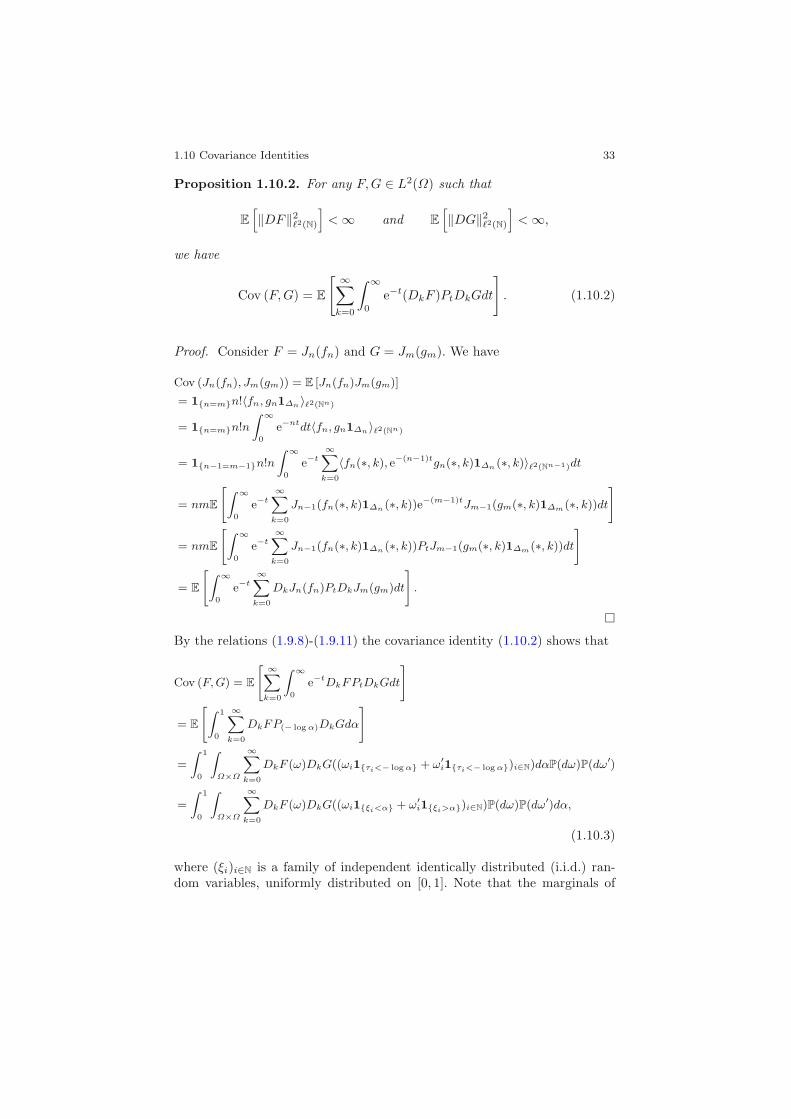
Proposition 1.10.2. For any F,G ∈ L2(Ω) such that
E
[‖DF‖2
�2(N)
]<∞ and E
[‖DG‖2
�2(N)
]<∞,
we have
Cov (F,G) = E
[ ∞∑
k=0
∫ ∞
0
e−t(DkF )PtDkGdt
]. (1.10.2)
Proof. Consider F = Jn(fn) and G = Jm(gm). We have
Cov (Jn(fn), Jm(gm)) = E [Jn(fn)Jm(gm)]
= 1{n=m}n!〈fn, gn1Δn 〉�2(Nn)
= 1{n=m}n!n
∫ ∞
0
e−ntdt〈fn, gn1Δn〉�2(Nn)
= 1{n−1=m−1}n!n
∫ ∞
0
e−t∞∑
k=0
〈fn(∗, k), e−(n−1)tgn(∗, k)1Δn (∗, k)〉�2(Nn−1)dt
= nmE
[∫ ∞
0
e−t∞∑
k=0
Jn−1(fn(∗, k)1Δn (∗, k))e−(m−1)tJm−1(gm(∗, k)1Δm(∗, k))dt
]
= nmE
[∫ ∞
0
e−t∞∑
k=0
Jn−1(fn(∗, k)1Δn (∗, k))PtJm−1(gm(∗, k)1Δm(∗, k))dt
]
= E
[∫ ∞
0
e−t∞∑
k=0
DkJn(fn)PtDkJm(gm)dt
].
�By the relations (1.9.8)-(1.9.11) the covariance identity (1.10.2) shows that
Cov (F, G) = E
[ ∞∑
k=0
∫ ∞
0
e−tDkFPtDkGdt
]
= E
[∫ 1
0
∞∑
k=0
DkFP(− log α)DkGdα
]
=
∫ 1
0
∫
Ω×Ω
∞∑
k=0
DkF (ω)DkG((ωi1{τi<− log α} + ω′i1{τi<− log α})i∈N)dαP(dω)P(dω′)
=
∫ 1
0
∫
Ω×Ω
∞∑
k=0
DkF (ω)DkG((ωi1{ξi<α} + ω′i1{ξi>α})i∈N)P(dω)P(dω′)dα,
(1.10.3)
where (ξi)i∈N is a family of independent identically distributed (i.i.d.) ran-dom variables, uniformly distributed on [0, 1]. Note that the marginals of

34 1 The Discrete Time Case
(Xk, Xk1{ξk<α} +X ′k1{ξi>α}) are identical when X ′k is an independent copyof Xk. Letting
φα(s, t) = E
[eisXkeit(Xk+1{ξk<α})+it(X′
k+1{ξk>α})],
we have the relation
Cov (eisXk , eitXk ) = φ1(s, t) − φ0(s, t)
=∫ 1
0
dφα
dα(s, t)dα.
Next we prove an iterated version of the covariance identity in discrete time,which is an analog of a result proved in [56] for the Wiener and Poissonprocesses.
Theorem 1.10.3. Let n ∈ N and F,G ∈ L2(Ω). We have
Cov (F,G) (1.10.4)
=n∑
d=1
(−1)d+1E
⎡
⎣∑
{1≤k1<···<kd}(Dkd
· · ·Dk1F )(Dkd· · ·Dk1G)
⎤
⎦
+(−1)nE
⎡
⎣∑
{1≤k1<···<kn+1}(Dkn+1 · · ·Dk1F )E
[Dkn+1 · · ·Dk1G | Fkn+1−1
]⎤
⎦.
Proof. Take F = G. For n = 0, (1.10.4) is a consequence of the Clark formula.Let n ≥ 1. Applying Lemma 1.7.4 to Dkn · · ·Dk1F with a = kn and b = kn+1,and summing on (k1, . . . , kn) ∈ Δn, we obtain
E
⎡
⎣∑
{1≤k1<···<kn}(E[Dkn · · ·Dk1F | Fkn−1])
2
⎤
⎦
= E
⎡
⎣∑
{1≤k1<···<kn}| Dkn · · ·Dk1F |2
⎤
⎦
−E
⎡
⎣∑
{1≤k1<···<kn+1}
(E[Dkn+1 · · ·Dk1F | Fkn+1−1
])2⎤
⎦ ,
which concludes the proof by induction and polarization. �As a consequence of Theorem 1.10.3, letting F =G we get the variance in-equality

1.10 Covariance Identities 35
2n∑
k=1
(−1)k+1
k!E
[‖DkF‖2
�2(Δk)
]≤ Var (F ) ≤
2n−1∑
k=1
(−1)k+1
k!E
[‖DkF‖2
�2(Δk)
],
since
E
⎡
⎣∑
{1≤k1<···<kn+1}(Dkn+1 · · ·Dk1F )E
[Dkn+1 · · ·Dk1F | Fkn+1−1
]⎤
⎦
= E
⎡
⎣∑
{1≤k1<···<kn+1}
E[(Dkn+1 · · ·Dk1F )E
[Dkn+1 · · ·Dk1F | Fkn+1−1
] | Fkn+1−1
] ]
= E
⎡
⎣∑
{1≤k1<···<kn+1}(E[Dkn+1 · · ·Dk1F | Fkn+1−1
])2
⎤
⎦
≥ 0,
see Relation (2.15) in [56] in continuous time. In a similar way, another iter-ated covariance identity can be obtained from Proposition 1.10.2.
Corollary 1.10.4. Let n ∈ N and F,G ∈ L2(Ω,FN ). We have
Cov (F,G) =n∑
d=1
(−1)d+1E
⎡
⎣∑
{1≤k1<···<kd≤N}(Dkd
· · ·Dk1F )(Dkd· · ·Dk1G)
⎤
⎦
+(−1)n
∫
Ω×Ω
∑
{1≤k1<···<kn+1≤N}Dkn+1 · · ·Dk1F (ω)Dkn+1 · · ·Dk1G(ω′)
qNt (ω, ω′)P(dω)P(dω′). (1.10.5)
Using the tensorization property
Var (FG) = E[F 2]Var (G) + (E[G])2Var (F )
≤ E[F 2Var (G)] + E[G2Var (F )]
of the variance for independent random variable F,G, most of the identities inthis section can be obtained by tensorization of elementary one dimensionalcovariance identities.The following lemma is an elementary consequence of the covariance identityproved in Proposition 1.10.1.
36 1 The Discrete Time Case
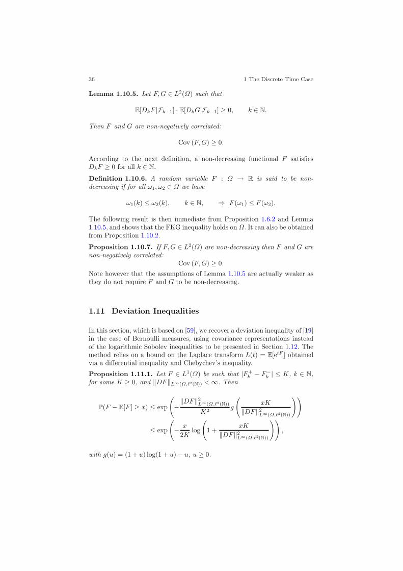
Lemma 1.10.5. Let F,G ∈ L2(Ω) such that
E[DkF |Fk−1] · E[DkG|Fk−1] ≥ 0, k ∈ N.
Then F and G are non-negatively correlated:
Cov (F,G) ≥ 0.
According to the next definition, a non-decreasing functional F satisfiesDkF ≥ 0 for all k ∈ N.
Definition 1.10.6. A random variable F : Ω → R is said to be non-decreasing if for all ω1, ω2 ∈ Ω we have
ω1(k) ≤ ω2(k), k ∈ N, ⇒ F (ω1) ≤ F (ω2).
The following result is then immediate from Proposition 1.6.2 and Lemma1.10.5, and shows that the FKG inequality holds on Ω. It can also be obtainedfrom Proposition 1.10.2.
Proposition 1.10.7. If F,G ∈ L2(Ω) are non-decreasing then F and G arenon-negatively correlated:
Cov (F,G) ≥ 0.
Note however that the assumptions of Lemma 1.10.5 are actually weaker asthey do not require F and G to be non-decreasing.
1.11 Deviation Inequalities
In this section, which is based on [59], we recover a deviation inequality of [19]in the case of Bernoulli measures, using covariance representations insteadof the logarithmic Sobolev inequalities to be presented in Section 1.12. Themethod relies on a bound on the Laplace transform L(t) = E[etF ] obtainedvia a differential inequality and Chebychev’s inequality.
Proposition 1.11.1. Let F ∈ L1(Ω) be such that |F+k − F−k | ≤ K, k ∈ N,
for some K ≥ 0, and ‖DF‖L∞(Ω,�2(N)) <∞. Then
P(F − E[F ] ≥ x) ≤ exp
(−‖DF‖2
L∞(Ω,�2(N))
K2g
(xK
‖DF‖2L∞(Ω,�2(N))
))
≤ exp
(− x
2Klog
(1 +
xK
‖DF‖2L∞(Ω,�2(N))
)),
with g(u) = (1 + u) log(1 + u) − u, u ≥ 0.

1.11 Deviation Inequalities 37
Proof. Although Dk does not satisfy a derivation rule for products, fromProposition 1.6.4 we have
DkeF = 1{Xk=1}√pkqk(eF − eF−
k ) + 1{Xk=−1}√pkqk(eF+
k − eF )
= 1{Xk=1}√pkqkeF (1 − e−
1√pkqk
DkF ) + 1{Xk=−1}√pkqkeF (e
1√pkqk
DkF − 1)
= −Xk√pkqkeF (e−
Xk√pkqk
DkF − 1),
hence
DkeF = Xk√pkqkeF (1 − e−
Xk√pkqk
DkF ), (1.11.1)
and since the function x → (ex − 1)/x is positive and increasing on R wehave:
e−sFDkesF
DkF= −Xk
√pkqk
DkF
(e−s
Xk√pkqk
DkF − 1)
≤ esK − 1K
,
or in other terms:
e−sFDkesF
DkF= 1{Xk=1}
esF−k −F+
k − 1F−k − F+
k
+ 1{Xk=−1}esF+
k −F−k − 1
F+k − F−k
≤ esK − 1K
.
We first assume that F is a bounded random variable with E[F ] = 0. FromProposition 1.10.2 applied to F and esF , noting that since F is bounded,
E
[‖DesF ‖2
�2(N)
]≤ CKE[e2sF ]‖DF‖2
L∞(Ω,�2(N))
< ∞,
for some CK > 0, we have
E[F esF ] = Cov (F, esF )
= E
[∫ ∞
0
e−v∞∑
k=0
DkesFPvDkFdv
]
≤∥∥∥∥
e−sFDesF
DF
∥∥∥∥∞
E
[esF
∫ ∞
0
e−v‖DFPvDF‖�1(N)dv
]

38 1 The Discrete Time Case
≤ esK − 1K
E
[esF ‖DF‖�2(N)
∫ ∞
0
e−v‖PvDF‖�2(N)dv
]
≤ esK − 1K
E[esF] ‖DF‖2
L∞(Ω,�2(N))
∫ ∞
0
e−vdv
≤ esK − 1K
E[esF] ‖DF‖2
L∞(Ω,�2(N)),
where we also applied Lemma 1.9.4 to u = DF .In the general case, letting L(s) = E[es(F−E[F ])], we have
log(E[et(F−E[F ])]) =∫ t
0
L′(s)L(s)
ds
≤∫ t
0
E[(F − E[F ])es(F−E[F ])]E[es(F−E[F ])]
ds
≤ 1K
‖DF‖2L∞(Ω,�2(N))
∫ t
0
(esK − 1)ds
=1K2
(etK − tK − 1)‖DF‖2L∞(Ω,�2(N)),
t ≥ 0. We have for all x ≥ 0 and t ≥ 0:
P(F − E[F ] ≥ x) ≤ e−txE[et(F−E[F ])]
≤ exp(
1K2
(etK − tK − 1)‖DF‖2L∞(Ω,�2(N)) − tx
),
The minimum in t ≥ 0 in the above expression is attained with
t =1K
log
(1 +
xK
‖DF‖2L∞(Ω,�2(N))
),
hence
P(F − E[F ] ≥ x)
≤ exp
(− 1K
(x+
‖DF‖2L∞(Ω,�2(N))
K
)log
(1 +
Kx
‖DF‖2L∞(Ω,�2(N))
)− x
K
)
≤ exp(− x
2Klog(1 + xK‖DF‖−2
L∞(Ω,�2(N))
)),
1.11 Deviation Inequalities 39
where we used the inequality
u
2log(1 + u) ≤ (1 + u) log(1 + u) − u, u ∈ R+.
If K =0, the above proof is still valid by replacing all terms by their lim-its as K→ 0. Finally if F is not bounded the conclusion holds for Fn =max(−n,min(F, n)), n ≥ 1, and (Fn)n∈N, (DFn)n∈N, converge respectivelyalmost surely and in L2(Ω × N) to F and DF , with ‖DFn‖2
L∞(Ω,L2(N)) ≤‖DF‖2
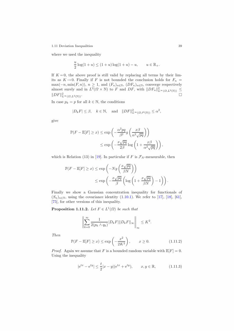
L∞(Ω,L2(N)). �In case pk = p for all k ∈ N, the conditions
|DkF | ≤ β, k ∈ N, and ‖DF‖2L∞(Ω,�2(N)) ≤ α2,
give
P(F − E[F ] ≥ x) ≤ exp(−α
2pq
β2g
(xβ
α2√pq))
≤ exp(−x
√pq
2βlog(
1 +xβ
α2√pq))
,
which is Relation (13) in [19]. In particular if F is FN -measurable, then
P(F − E[F ] ≥ x) ≤ exp(−Ng
(x√pq
βN
))
≤ exp(−x
√pq
β
(log(
1 +x√pq
βN
)− 1))
.
Finally we show a Gaussian concentration inequality for functionals of(Sn)n∈N, using the covariance identity (1.10.1). We refer to [17], [18], [61],[75], for other versions of this inequality.
Proposition 1.11.2. Let F ∈ L1(Ω) be such that
∥∥∥∥∥
∞∑
k=0
12(pk ∧ qk)
|DkF |‖DkF‖∞∥∥∥∥∥∞
≤ K2.
Then
P(F − E[F ] ≥ x) ≤ exp(− x2
2K2
), x ≥ 0. (1.11.2)
Proof. Again we assume that F is a bounded random variable with E[F ] = 0.Using the inequality
|etx − ety| ≤ t
2|x− y|(etx + ety), x, y ∈ R, (1.11.3)

40 1 The Discrete Time Case
we have
|DketF | =√pkqk|etF+
k − etF−k |
≤ 12√pkqkt|F+
k − F−k |(etF+k + etF−
k )
=12t|DkF |(etF+
k + etF−k )
≤ t
2(pk ∧ qk)|DkF |E
[etF | Xi, i �= k
]
=1
2(pk ∧ qk)tE[etF |DkF | | Xi, i �= k
].
Now Proposition 1.10.1 yields
E[F etF ] = Cov (F, esF )
=∞∑
k=0
E[E[DkF | Fk−1]DketF ]
≤∞∑
k=0
‖DkF‖∞E[|DketF |]
≤ t
2
∞∑
k=0
1pk ∧ qk ‖DkF‖∞E
[E[etF |DkF | | Xi, i �= k
]]
=t
2E
[etF
∞∑
k=0
1pk ∧ qk ‖DkF‖∞|DkF |
]
≤ t
2E[etF ]
∥∥∥∥∥
∞∑
k=0
1pk ∧ qk |DkF |‖DkF‖∞
∥∥∥∥∥∞.
This shows that
log(E[et(F−E[F ])]) =∫ t
0
E[(F − E[F ])es(F−E[F ])]E[es(F−E[F ])]
ds
≤ K2
∫ t
0
sds
=t2
2K2,
hence
exP(F − E[F ] ≥ x) ≤ E[et(F−E[F ])]
≤ et2K2/2, t ≥ 0,

1.11 Deviation Inequalities 41
andP(F − E[F ] ≥ x) ≤ e
t22 K2−tx, t ≥ 0.
The best inequality is obtained for t = x/K2.Finally if F is not bounded the conclusion holds for Fn = max(−n,min(F, n)), n ≥ 0, and (Fn)n∈N, (DFn)n∈N, converge respectively to F and DFin L2(Ω), resp. L2(Ω × N), with ‖DFn‖2
L∞(Ω,�2(N)) ≤ ‖DF‖2L∞(Ω,�2(N)). �
In case pk = p, k ∈ N, we obtain
P(F − E[F ] ≥ x) ≤ exp
(− px2
‖DF‖2�2(N,L∞(Ω))
).
Proposition 1.11.3. We have E[eα|F |] <∞ for all α > 0, and E[eαF 2] <∞
for all α < 1/(2K2).
Proof. Let λ < c/e. The bound (1.11.2) implies
IE[eα|F |]
=∫ ∞
0
P(eα|F | ≥ t)dt
=∫ ∞
−∞P(α|F | ≥ y)eydy
≤ 1 +∫ ∞
0
P(α|F | ≥ y)eydy
≤ 1 +∫ ∞
0
exp(− (IE[|F |] + y/α)2
2K2
)eydy
< ∞,
for all α > 0. On the other hand we have
IE[eαF 2] =∫ ∞
0
P(eαF 2 ≥ t)dt
=∫ ∞
−∞P(αF 2 ≥ y)eydy
≤ 1 +∫ ∞
0
P(|F | ≥ (y/α)1/2)eydy
≤ 1 +∫ ∞
0
exp(− (IE[|F |] + (y/α)1/2)2
2K2
)eydy
< ∞,
provided 2K2α < 1. �

42 1 The Discrete Time Case
1.12 Logarithmic Sobolev Inequalities
The logarithmic Sobolev inequalities on Gaussian space provide an infinitedimensional analog of Sobolev inequalities, cf. e.g. [77]. On Riemannianpath space [22] and on Poisson space [6], [151], martingale methods havebeen successfully applied to the proof of logarithmic Sobolev inequalities.Here, discrete time martingale methods are used along with the Clark pre-dictable representation formula (1.7.1) as in [46], to provide a proof oflogarithmic Sobolev inequalities for Bernoulli measures. Here we are onlyconcerned with modified logarithmic Sobolev inequalities, and we refer to[127], Theorem 2.2.8 and references therein, for the standard version of thelogarithmic Sobolev inequality on the hypercube under Bernoulli measures.The entropy of a random variable F > 0 is defined by
Ent [F ] = E[F logF ] − E[F ] log E[F ],
for sufficiently integrable F .
Lemma 1.12.1. The entropy has the tensorization property, i.e. if F,G aresufficiently integrable independent random variables we have
Ent [FG] = E[FEnt [G]] + E[GEnt [F ]]. (1.12.1)
Proof. We have
Ent [FG] = E[FG log(FG)] − E[FG] log E[FG]= E[FG(logF + logG)] − E[F ]E[G](log E[F ] + log E[G])= E[G]E[F logF ] + E[F ]E[G logG)] − E[F ]E[G](log E[F ] + log E[G])= E[FEnt [G]] + E[GEnt [F ]].
�In the next proposition we recover the modified logarithmic Sobolev inequal-ity of [19] using the Clark representation formula in discrete time.
Theorem 1.12.2. Let F ∈ Dom (D) with F > η a.s. for some η > 0. Wehave
Ent [F ] ≤ E
[1F‖DF‖2
�2(N)
]. (1.12.2)
Proof. Assume that F is FN -measurable and letMn = E[F | Fn], 0 ≤ n ≤ N .Using Corollary 1.6.3 and the Clark formula (1.7.1) we have
Mn = M−1 +n∑
k=0
ukYk, 0 ≤ n ≤ N,
with uk = E[DkF | Fk−1], 0 ≤ k ≤ n ≤ N , and M−1 = E[F ]. Lettingf(x) = x log x and using the bound

1.12 Logarithmic Sobolev Inequalities 43
f(x+ y) − f(x) = y log x+ (x+ y) log(1 +
y
x
)
≤ y(1 + log x) +y2
x,
we have:
Ent [F ] = E[f(MN)] − E[f(M−1)]
= E
[N∑
k=0
f(Mk) − f(Mk−1)
]
= E
[N∑
k=0
f (Mk−1 + Ykuk) − f(Mk−1)
]
≤ E
[N∑
k=0
Ykuk(1 + logMk−1) +Y 2
k u2k
Mk−1
]
= E
[N∑
k=0
1E[F | Fk−1]
(E[DkF | Fk−1])2]
≤ E
[N∑
k=0
E
[1F|DkF |2 | Fk−1
]]
= E
[1F
N∑
k=0
|DkF |2].
where we used the Jensen inequality (9.3.1) and the convexity of (u, v) →v2/u on (0,∞) × R, or the Schwarz inequality applied to
1/√F and (DkF/
√F )k∈N,
as in the Wiener and Poisson cases [22] and [6]. This inequality is extendedby density to F ∈ Dom(D). �By a one-variable argument, letting df = f(1) − f(−1), we have
Ent [f ] = pf(1) log f(1) + qf(−1) log f(−1)− E[f ] log E[f ]= p(E[f ] + qdf) log(E[f ] + qdf)
+q(E[f ] − pdf) log(E[f ] − pdf) − (pf(1) + qf(−1)) log E[f ]
= pE[f ] log(
1 + qdf
E[f ]
)+ pqdf log f(1)
+qE[f ] log(
1 − pdf
E[f ]
)− qpdf log f(−1)
≤ pqdf log f(1) − pqdf log f(−1)= pqE [dfd log f ] ,

44 1 The Discrete Time Case
which, by tensorization, recovers the following L1 inequality of [47], [29], andproved in [151] in the Poisson case. In the next proposition we state and provethis inequality in the multidimensional case, using the Clark representationformula, similarly to Theorem 1.12.2.
Theorem 1.12.3. Let F > 0 be FN -measurable. We have
Ent [F ] ≤ E
[N∑
k=0
DkFDk logF
]. (1.12.3)
Proof. Let f(x) = x log x and
Ψ(x, y) = (x + y) log(x+ y) − x log x− (1 + log x)y, x, x+ y > 0.
From the relation
Ykuk = YkE[DkF | Fk−1]
= qk1{Xk=1}E[(F+k − F−k ) | Fk−1] + pk1{Xk=−1}E[(F−k − F+
k ) | Fk−1]
= 1{Xk=1}E[(F+k − F−k )1{Xk=−1} | Fk−1]
+1{Xk=−1}E[(F−k − F+k )1{Xk=1} | Fk−1],
we have, using the convexity of Ψ :
Ent [F ] = E
[N∑
k=0
f (Mk−1 + Ykuk) − f(Mk−1)
]
= E
[N∑
k=0
Ψ(Mk−1, Ykuk) + Ykuk(1 + log Mk−1)
]
= E
[N∑
k=0
Ψ(Mk−1, Ykuk)
]
= E
[N∑
k=0
pkΨ(E[F | Fk−1], E[(F+
k − F−k )1{Xk=−1} | Fk−1]
)
+qkΨ(E[F | Fk−1], E[(F−
k − F+k )1{Xk=1} | Fk−1]
)]
≤ E
[N∑
k=0
E
[pkΨ(F, (F+
k − F−k )1{Xk=−1}
)+ qkΨ
(F, (F−
k − F+k )1{Xk=1}
) ∣∣∣Fk−1
]]
= E
[N∑
k=0
pk1{Xk=−1}Ψ(F−
k , F+k − F−
k
)+ qk1{Xk=1}Ψ
(F+
k , F−k − F+
k
)]

1.12 Logarithmic Sobolev Inequalities 45
= E
[N∑
k=0
pkqkΨ(F−k , F+
k − F−k ) + pkqkΨ(F+
k , F−k − F+
k )
]
= E
[N∑
k=0
pkqk(log F+k − log F−
k )(F+k − F−
k )
]
= E
[N∑
k=0
DkFDk log F
].
�The application of Theorem 1.12.3 to eF gives the following inequality forF > 0, FN -measurable:
Ent [eF ] ≤ E
[N∑
k=0
DkFDkeF
]
= E
[N∑
k=0
pkqkΨ(eF−k , eF+
k − eF−k ) + pkqkΨ(eF+
k , eF−k − eF+
k )
]
= E
[N∑
k=0
pkqkeF−k ((F+
k − F−k )eF+k −F−
k − eF+k −F−
k + 1)
+pkqkeF+k ((F−k − F+
k )eF−k−F+
k − eF−k−F+
k + 1)]
= E
[N∑
k=0
pk1{Xk=−1}eF−k ((F+
k − F−k )eF+k −F−
k − eF+k −F−
k + 1)
+qk1{Xk=1}eF+k ((F−k − F+
k )eF−k−F+
k − eF−k−F+
k + 1)]
= E
[eF
N∑
k=0
√pkqk|Yk|(∇kF e∇kF − e∇kF + 1)
]. (1.12.4)
This implies
Ent [eF ] ≤ E
[eF
N∑
k=0
(∇kF e∇kF − e∇kF + 1)
]. (1.12.5)
As noted in [29], Relation (1.12.3) and the Poisson limit theorem yield the L1
inequality of [151]. More precisely, letting Mn = (n+X1 + · · ·+Xn)/2, F =ϕ(Mn) and pk = λ/n, k ∈ N, , n ≥ 1, λ > 0, we have, from Proposition 1.6.2,

46 1 The Discrete Time Case
n∑
k=0
DkFDk logF
=λ
n
(1 − λ
n
)(n−Mn)(ϕ(Mn + 1) − ϕ(Mn)) log(ϕ(Mn + 1) − ϕ(Mn))
+λ
n
(1 − λ
n
)Mn(ϕ(Mn) − ϕ(Mn − 1)) log(ϕ(Mn) − ϕ(Mn − 1)),
in the limit as n goes to infinity we obtain
Ent [ϕ(U)] ≤ λE[(ϕ(U + 1) − ϕ(U))(logϕ(U + 1) − logϕ(U))],
where U is a Poisson random variable with parameter λ. In one variable wehave, still letting df = f(1) − f(−1),
Ent [ef ] ≤ pqE[defd log ef
]
= pq(ef(1) − ef(−1))(f(1) − f(−1))= pqef(−1)((f(1) − f(−1))ef(1)−f(−1) − ef(1)−f(−1) + 1)
+pqef(1)((f(−1) − f(1))ef(−1)−f(1) − ef(−1)−f(1) + 1)≤ qef(−1)((f(1) − f(−1))ef(1)−f(−1) − ef(1)−f(−1) + 1)
+pef(1)((f(−1) − f(1))ef(−1)−f(1) − ef(−1)−f(1) + 1)= E[ef (∇fe∇f − e∇f + 1)
],
where ∇k is the gradient operator defined in (1.6.4). This last inequality isnot comparable to the optimal constant inequality
Ent [eF ] ≤ E
[eF
N∑
k=0
pkqk(|∇kF |e|∇kF | − e|∇kF | + 1)
], (1.12.6)
of [19] since when F+k − F−k ≥ 0 the right-hand side of (1.12.6) grows as
F+k e2F+
k , instead of F+k eF+
k in (1.12.5). In fact we can prove the followinginequality which improves (1.12.2), (1.12.3) and (1.12.6).
Theorem 1.12.4. Let F be FN -measurable. We have
Ent [eF ] ≤ E
[eF
N∑
k=0
pkqk(∇kF e∇kF − e∇kF + 1)
]. (1.12.7)
Clearly, (1.12.7) is better than (1.12.6), (1.12.4) and (1.12.3). It also improves(1.12.2) from the bound
xex − ex + 1 ≤ (ex − 1)2, x ∈ R,
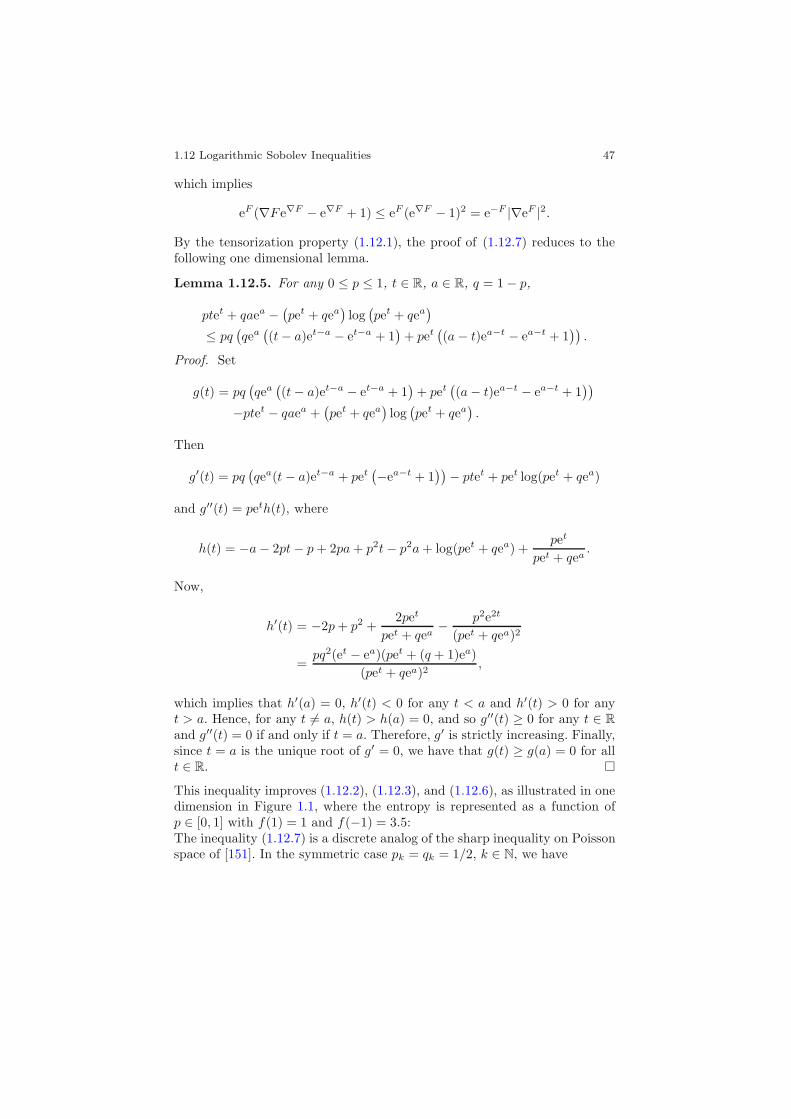
1.12 Logarithmic Sobolev Inequalities 47
which implies
eF (∇F e∇F − e∇F + 1) ≤ eF (e∇F − 1)2 = e−F |∇eF |2.
By the tensorization property (1.12.1), the proof of (1.12.7) reduces to thefollowing one dimensional lemma.
Lemma 1.12.5. For any 0 ≤ p ≤ 1, t ∈ R, a ∈ R, q = 1 − p,
ptet + qaea − (pet + qea)log(pet + qea
)
≤ pq(qea((t− a)et−a − et−a + 1
)+ pet
((a− t)ea−t − ea−t + 1
)).
Proof. Set
g(t) = pq(qea((t− a)et−a − et−a + 1
)+ pet
((a− t)ea−t − ea−t + 1
))
−ptet − qaea +(pet + qea
)log(pet + qea
).
Then
g′(t) = pq(qea(t− a)et−a + pet
(−ea−t + 1))− ptet + pet log(pet + qea)
and g′′(t) = peth(t), where
h(t) = −a− 2pt− p+ 2pa+ p2t− p2a+ log(pet + qea) +pet
pet + qea.
Now,
h′(t) = −2p+ p2 +2pet
pet + qea− p2e2t
(pet + qea)2
=pq2(et − ea)(pet + (q + 1)ea)
(pet + qea)2,
which implies that h′(a) = 0, h′(t) < 0 for any t < a and h′(t) > 0 for anyt > a. Hence, for any t �= a, h(t) > h(a) = 0, and so g′′(t) ≥ 0 for any t ∈ R
and g′′(t) = 0 if and only if t = a. Therefore, g′ is strictly increasing. Finally,since t = a is the unique root of g′ = 0, we have that g(t) ≥ g(a) = 0 for allt ∈ R. �This inequality improves (1.12.2), (1.12.3), and (1.12.6), as illustrated in onedimension in Figure 1.1, where the entropy is represented as a function ofp ∈ [0, 1] with f(1) = 1 and f(−1) = 3.5:The inequality (1.12.7) is a discrete analog of the sharp inequality on Poissonspace of [151]. In the symmetric case pk = qk = 1/2, k ∈ N, we have

48 1 The Discrete Time Case
0
2
4
6
8
10
12
14
16
18
0.2 0.4 0.6 0.8 1p
optimal
modified
L1
sharp
entropy
Fig. 1.1 Graph of bounds on the entropy as a function of p ∈ [0, 1]
Ent [eF ] ≤ E
[eF
N∑
k=0
pkqk(∇kF e∇kF −∇kF + 1)
]
=18
E
[N∑
k=0
eF−k ((F+
k − F−k )eF+k −F−
k − eF+k −F−
k + 1)
+eF+k ((F−k − F+
k )eF−k −F+
k − eF−k −F+
k + 1)]
=18
E
[N∑
k=0
(eF+k − eF−
k )(F+k − F−k )
]
=12
E
[N∑
k=0
DkFDkeF
],
which improves on (1.12.3).Similarly the sharp inequality of [151] can be recovered by taking F = ϕ(Mn)in
Ent [eF ] ≤ E
[eF
N∑
k=0
pkqk(∇kF e∇kF −∇kF + 1)
]
=λ
n
(1 − λ
n
)E
[Mneϕ(Mn)
× ((ϕ(Mn) − ϕ(Mn − 1))eϕ(Mn)−ϕ(Mn−1) − eϕ(Mn)−ϕ(Mn−1) + 1)]
+λ
n
(1 − λ
n
)E
[(n−Mn)eϕ(Mn)
× ((ϕ(Mn + 1) − ϕ(Mn))eϕ(Mn+1)−ϕ(Mn) − eϕ(Mn+1)−ϕ(Mn) + 1)],

1.13 Change of Variable Formula 49
which, in the limit as n goes to infinity, yields
Ent [eϕ(U)] ≤ λE[eϕ(U)((ϕ(U + 1)− ϕ(U))eϕ(U+1)−ϕ(U) − eϕ(U+1)−ϕ(U) + 1)],
where U is a Poisson random variable with parameter λ.
1.13 Change of Variable Formula
In this section we state a discrete-time analog of Ito’s change of variableformula which will be useful for the predictable representation of randomvariables and for option hedging.
Proposition 1.13.1. Let (Mn)n∈N be a square-integrable martingale and f :R × N → R. We have
f(Mn, n)
= f(M−1,−1)+n∑
k=0
Dkf(Mk, k)Yk+n∑
k=0
E[f(Mk, k)−f(Mk−1, k − 1) | Fk−1]
+n∑
k=0
f(Mk−1, k) − f(Mk−1, k − 1). (1.13.1)
Proof. By Proposition 1.7.5 there exists square-integrable process (uk)k∈N
such that
Mn = M−1 +n∑
k=0
ukYk, n ∈ N.
We write
f(Mn, n) − f(M−1,−1) =n∑
k=0
f(Mk, k) − f(Mk−1, k − 1)
=n∑
k=0
f(Mk, k) − f(Mk−1, k) + f(Mk−1, k) − f(Mk−1, k − 1)
=n∑
k=0
√pk
qk
(f
(Mk−1 + uk
√qkpk, k
)− f(Mk−1, k)
)Yk
+pk
qk1{Xk=−1}
(f
(Mk−1 + uk
√qkpk, k
)− f(Mk−1, k)
)
+1{Xk=−1}
(f
(Mk−1 − uk
√pk
qk, k
)− f(Mk−1, k)
)
+n∑
k=0
f(Mk−1, k) − f(Mk−1, k − 1)
50 1 The Discrete Time Case
=n∑
k=0
√pk
qk
(f
(Mk−1 + uk
√qkpk, k
)− f(Mk−1, k)
)Yk
+n∑
k=0
1qk
1{Xk=−1}E[f(Mk, k) − f(Mk−1, k) | Fk−1]
+n∑
k=0
f(Mk−1, k) − f(Mk−1, k − 1).
Similarly we have
f(Mn, n)
= f(M−1,−1) −n∑
k=0
√qkpk
(f
(Mk−1 − uk
√pk
qk, k
)− f(Mk−1, k)
)Yk
+n∑
k=0
1pk
1{Xk=1}E[f(Mk, k) − f(Mk−1, k) | Fk−1]
+n∑
k=0
f(Mk−1, k) − f(Mk−1, k − 1).
Multiplying each increment in the above formulas respectively by qk and pk
and summing on k we get
f(Mn, n) = f(M−1,−1) +n∑
k=0
f(Mk, k) − f(Mk−1, k − 1)
= f(M−1,−1) +n∑
k=0
qk(f(Mk, k) − f(Mk−1, k − 1))
+n∑
k=0
pk(f(Mk, k) − f(Mk−1, k − 1))
= f(M−1,−1) +n∑
k=0
√pkqk
(f
(Mk−1 + uk
√qkpk, k
)− f(Mk−1, k)
)Yk
−n∑
k=0
√pkqk
(f
(Mk−1 − uk
√pk
qk, k
)− f(Mk−1, k)
)Yk
+n∑
k=0
E[f(Mk, k) | Fk−1] − f(Mk−1, k − 1)
+n∑
k=0
f(Mk−1, k) − f(Mk−1, k − 1)
= f(M−1,−1)
1.13 Change of Variable Formula 51
+n∑
k=0
√pkqk
(f
(Mk−1 + uk
√qkpk, k
)− f
(Mk−1 − uk
√pk
qk, k
))Yk
+n∑
k=0
E[f(Mk, k) | Fk−1] − f(Mk−1, k − 1)
+n∑
k=0
f(Mk−1, k) − f(Mk−1, k − 1).
�Note that in (1.13.1) we have
Dkf(Mk, k) =√pkqk
(f
(Mk−1 + uk
√qkpk, k
)− f
(Mk−1 − uk
√pk
qk, k
)),
k ∈ N.On the other hand, the term
E[f(Mk, k) − f(Mk−1, k − 1) | Fk−1]
is analog to the generator part in the continuous time Ito formula, and canbe written as
pkf
(Mk−1 + uk
√qkpk, k
)+ qkf
(Mk−1 − uk
√pk
qk, k
)− f (Mk−1, k − 1) .
When pn = qn = 1/2, n ∈ N, we have
f(Mn, n) = f(M−1,−1) +n∑
k=0
f (Mk−1 + uk, k) − f (Mk−1 − uk, k)2
Yk
+n∑
k=0
f (Mk−1 + uk, k) − f (Mk−1 − uk, k) − 2f (Mk−1 − uk, k)2
+n∑
k=0
f(Mk−1, k) − f(Mk−1, k − 1).
The above proposition also provides an explicit version of the Doob decom-position for supermartingales. Naturally if (f(Mn, n))n∈N is a martingale wehave
52 1 The Discrete Time Case
f(Mn, n) = f(M−1,−1)
+n∑
k=0
√pkqk
(f
(Mk−1 + uk
√qkpk, k
)− f
(Mk−1 − uk
√pk
qk, k
))Yk
= f(M−1,−1) +n∑
k=0
Dkf(Mk, k)Yk.
In this case the Clark formula, the martingale representation formulaProposition 1.7.5 and the change of variable formula all coincide. In thiscase, we have in particular
Dkf(Mk, k) = E[Dkf(Mn, n) | Fk−1]
= E[Dkf(Mk, k) | Fk−1], k ∈ N.
If F is an FN -measurable random variable and f is a function such that
E[F | Fn] = f(Mn, n), −1 ≤ n ≤ N,
we have F = f(MN , N), E[F ] = f(M−1,−1) and
F = E[F ] +n∑
k=0
E[Dkf(MN , N) | Fk−1]Yk
= E[F ] +n∑
k=0
Dkf(Mk, k)Yk
= E[F ] +n∑
k=0
DkE[f(MN , N) | Fk]Yk.
Such a function f exists if (Mn)n∈N is Markov and F = h(MN). In thiscase, consider the semi-group (Pk,n)0≤k<n≤N associated to (Mn)n∈N and de-fined by
(Pk,nh)(x) = E[h(Mn) |Mk = x].
Letting f(x, n) = (Pn,Nh)(x) we can write
F = E[F ] +n∑
k=0
E[Dkh(MN ) | Fk−1]Yk
= E[F ] +n∑
k=0
Dk(Pk,Nh(Mk))Yk.

1.14 Option Hedging 53
1.14 Option Hedging
In this section we give a presentation of the Black-Scholes formula in discretetime, or Cox-Ross-Rubinstein model, see e.g. [45], [74], [125], or §15-1 of [149]as an application of the Clark formula.In order to be consistent with the notation of the previous sections we chooseto use the time scale N, hence the index 0 is that of the first random value ofany stochastic process, while the index −1 corresponds to its deterministicinitial value.Let (Ak)k∈N be a riskless asset with initial value A−1, and defined by
An = A−1
n∏
k=0
(1 + rk), n ∈ N,
where (rk)k∈N, is a sequence of deterministic numbers such that rk > − 1,k ∈ N. Consider a stock price with initial value S−1, given in discrete time as
Sn =
⎧⎨
⎩
(1 + bn)Sn−1 if Xn = 1,
(1 + an)Sn−1 if Xn = −1, n ∈ N,
where (ak)k∈N and (bk)k∈N are sequences of deterministic numbers such that
−1 < ak < rk < bk, k ∈ N.
We have
Sn = S−1
n∏
k=0
√(1 + bk)(1 + ak)
(1 + bk1 + ak
)Xk/2
, n ∈ N.
Consider now the discounted stock price given as
Sn = Sn
n∏
k=0
(1 + rk)−1
= S−1
n∏
k=0
(1
1 + rk
√(1 + bk)(1 + ak)
(1 + bk1 + ak
)Xk/2), n ∈ N.
If −1 < ak < rk < bk, k ∈ N, then (Sn)n∈N is a martingale with respect to(Fn)n≥−1 under the probability P
∗ given by
pk =rk − ak
bk − ak, qk =
bk − rkbk − ak
, k ∈ N.

54 1 The Discrete Time Case
In other terms, under P∗ we have
E∗[Sn+1 | Fn] = (1 + rn+1)Sn, n ≥ −1,
where E∗ denotes the expectation under P
∗. Recall that under this probabil-ity measure there is absence of arbitrage and the market is complete. Fromthe change of variable formula Proposition 1.13.1 or from the Clark formula(1.7.1) we have the martingale representation
Sn = S−1 +n∑
k=0
YkDkSk = S−1 +n∑
k=0
Sk−1√pkqk
bk − ak
1 + rkYk.
Definition 1.14.1. A portfolio strategy is represented by a pair of predictableprocesses (ηk)k∈N and (ζk)k∈N where ηk, resp. ζk represents the numbers ofunits invested over the time period (k, k + 1] in the asset Sk, resp. Ak, withk ≥ 0.
The value at time k ≥ −1 of the portfolio (ηk, ζk)0≤k≤N is defined as
Vk = ζk+1Ak + ηk+1Sk, k ≥ −1, (1.14.1)
and its discounted value is defined as
Vn = Vn
n∏
k=0
(1 + rk)−1, n ≥ −1. (1.14.2)
Definition 1.14.2. A portfolio (ηk, ζk)k∈N is said to be self-financing if
Ak(ζk+1 − ζk) + Sk(ηk+1 − ηk) = 0, k ≥ 0.
Note that the self-financing condition implies
Vk = ζkAk + ηkSk, k ≥ 0.
Our goal is to hedge an arbitrary claim onΩ, i.e. given an FN -measurable ran-dom variable F we search for a portfolio (ηk, ζk)0≤k≤n such that the equality
F = VN = ζNAN + ηNSN (1.14.3)
holds at time N ∈ N.
Proposition 1.14.3. Assume that the portfolio (ηk, ζk)0≤k≤N is self-financing. Then we have the decomposition
Vn = V−1
n∏
k=0
(1 + rk) +n∑
i=0
ηiSi−1√piqi(bi − ai)Yi
n∏
k=i+1
(1 + rk). (1.14.4)
1.14 Option Hedging 55
Proof. Under the self-financing assumption we have
Vi − Vi−1 = ζi(Ai −Ai−1) + ηi(Si − Si−1)= riζiAi−1 + (ai1{Xi=−1} + bi1{Xi=1})ηiSi−1
= ηiSi−1(ai1{Xi=−1} + bi1{Xi=1} − ri) + riVi−1
= ηiSi−1((ai − ri)1{Xi=−1} + (bi − ri)1{Xi=1}) + riVi−1
= (bi − ai)ηiSi−1(−pi1{Xi=−1} + qi1{Xi=1}) + riVi−1
= ηiSi−1√piqi(bi − ai)Yi + riVi−1, i ∈ N,
by Relation (1.4.5), hence for the discounted portfolio we get:
Vi − Vi−1 =i∏
k=1
(1 + rk)−1Vi −i−1∏
k=1
(1 + rk)−1Vi−1
=i∏
k=1
(1 + rk)−1(Vi − Vi−1 − riVi−1)
= ηiSi−1√piqi(bi − ai)Yi
i∏
k=1
(1 + rk)−1, i ∈ N,
which successively yields (1.14.4). �As a consequence of (1.14.4) and (1.14.2) we immediately obtain
Vn = V−1 +n∑
i=0
ηiSi−1√piqi(bi − ai)Yi
i∏
k=0
(1 + rk)−1, (1.14.5)
n ≥ −1. The next proposition provides a solution to the hedging problemunder the constraint (1.14.3).
Proposition 1.14.4. Given F ∈ L2(Ω,FN ), let
ηn =1
Sn−1√pnqn(bn − an)
E∗[DnF | Fn−1]
N∏
k=n+1
(1 + rk)−1, (1.14.6)
0 ≤ n ≤ N , and
ζn = A−1n
(N∏
k=n+1
(1 + rk)−1E∗[F | Fn] − ηnSn
), (1.14.7)

56 1 The Discrete Time Case
0 ≤ n ≤ N . Then the portfolio (ηk, ζk)0≤k≤n is self financing and satisfies
ζnAn + ηnSn =N∏
k=n+1
(1 + rk)−1E∗[F | Fn],
0 ≤ n ≤ N , in particular we have VN = F , hence (ηk, ζk)0≤k≤N is a hedgingstrategy leading to F .
Proof. Let (ηk)−1≤k≤N be defined by (1.14.6) and η−1 = 0, and consider theprocess (ζn)0≤n≤N defined by
ζ−1 =E∗[F ]S−1
N∏
k=0
(1 + rk)−1 and ζk+1 = ζk − (ηk+1 − ηk)Sk
Ak,
k = −1, . . . , N −1. Then (ηk, ζk)−1≤k≤N satisfies the self-financing condition
Ak(ζk+1 − ζk) + Sk(ηk+1 − ηk) = 0, −1 ≤ k ≤ N − 1.
Let now
V−1 = E∗[F ]
N∏
k=0
(1 + rk)−1, and Vn = ζnAn + ηnSn, 0 ≤ n ≤ N,
and
Vn = Vn
n∏
k=0
(1 + rk)−1, −1 ≤ n ≤ N.
Since (ηk, ζk)−1≤k≤N is self-financing, Relation (1.14.5) shows that
Vn = V−1 +n∑
i=0
YiηiSi−1√piqi(bi − ai)
i∏
k=1
(1 + rk)−1, (1.14.8)
−1 ≤ n ≤ N . On the other hand, from the Clark formula (1.7.1) and thedefinition of (ηk)−1≤k≤N we have
E∗[F | Fn]
N∏
k=0
(1 + rk)−1
= E∗[E∗[F ]
N∏
k=0
(1 + rk)−1 +N∑
i=0
YiE∗[DiF | Fi−1]
N∏
k=0
(1 + rk)−1∣∣∣Fn
]
= E∗[F ]
N∏
k=0
(1 + rk)−1 +n∑
i=0
YiE∗[DiF | Fi−1]
N∏
k=0
(1 + rk)−1

1.14 Option Hedging 57
= E∗[F ]
N∏
k=0
(1 + rk)−1 +n∑
i=0
YiηiSi−1√piqi(bi − ai)
i∏
k=1
(1 + rk)−1
= Vn
from (1.14.8). Hence
Vn = E∗[F | Fn]
N∏
k=0
(1 + rk)−1, −1 ≤ n ≤ N,
and
Vn = E∗[F | Fn]
N∏
k=n+1
(1 + rk)−1, −1 ≤ n ≤ N.
In particular we have VN = F . To conclude the proof we note that fromthe relation Vn = ζnAn + ηnSn, 0 ≤ n ≤ N , the process (ζn)0≤n≤N coincideswith (ζn)0≤n≤N defined by (1.14.7). �Note that we also have
ζn+1An + ηn+1Sn = E∗[F | Fn]
N∏
k=n+1
(1 + rk)−1, −1 ≤ n ≤ N.
The above proposition shows that there always exists a hedging strategystarting from
V−1 = E∗[F ]
N∏
k=0
(1 + rk)−1.
Conversely, if there exists a hedging strategy leading to
VN = FN∏
k=0
(1 + rk)−1,
then (Vn)−1≤n≤N is necessarily a martingale with initial value
V−1 = E∗[VN ] = E
∗[F ]N∏
k=0
(1 + rk)−1.
When F = h(SN ), we have E∗[h(SN ) | Fk] = f(Sk, k) with
f(x, k) = E∗[h
(x
n∏
i=k+1
√(1 + bk)(1 + ak)
1 + rk
(1 + bk1 + ak
)Xk/2)]
.
58 1 The Discrete Time Case
The hedging strategy is given by
ηk =1
Sk−1√pkqk(bk − ak)
Dkf(Sk, k)N∏
i=k+1
(1 + ri)−1
=∏N
i=k+1(1 + ri)−1
Sk−1(bk − ak)
(f
(Sk−1
1 + bk1 + rk
, k
)− f
(Sk−1
1 + ak
1 + rk, k
)),
k≥ − 1. Note that ηk is non-negative (i.e. there is no short-selling) whenf is an increasing function, e.g. in the case of European options we havef(x) = (x−K)+.
1.15 Notes and References
This chapter is a revision of [113] with some additions, and is mainly based on[59] and [115]. It is included for the sake of consistency and for the role it playsas an introduction to the next chapters. Other approaches to discrete-timestochastic analysis include [53], [54], [48], [78] and [89]; see [8] for an approachbased on quantum probability. Deviation inequalities and logarithmic Sobolevinequalities are treated in [19], [46], [59]. We also refer to [5], [17], [18], [61],[75], for other versions of logarithmic Sobolev inequalities in discrete settings.See [74], §15-1 of [149], and [125], for other derivations of the Black-Scholesformula in the discrete time Cox-Ross-Rubinstein model.
Chapter 2
Continuous Time Normal Martingales
This chapter is concerned with the basics of stochastic calculus in continuoustime. In continuation of Chapter 1 we keep considering the point of view ofnormal martingales and structure equations, which provides a unified treat-ment of stochastic integration and calculus that applies to both continuousand discontinuous processes. In particular we cover the construction of singleand multiple stochastic integrals with respect to normal martingales and wediscuss other classical topics such as quadratic variations and the Ito formula.
2.1 Normal Martingales
Let (Ω,F ,P) be a probability space equipped with a right-continuous filtra-tion (Ft)t∈R+ , i.e. an increasing family of sub σ-algebras of F such that
Ft =⋂
s>t
Fs, t ∈ R+.
We refer to Section 9.5 in the Appendix for recalls on martingales in conti-nuous time.
Definition 2.1.1. A square-integrable martingale (Mt)t∈R+ such that
E[(Mt −Ms)2|Fs
]= t− s, 0 ≤ s < t, (2.1.1)
is called a normal martingale.
Every square-integrable process (Mt)t∈R+ with centered independent incre-ments and generating the filtration (Ft)t∈R+ satisfies
E[(Mt −Ms)2|Fs
]= E
[(Mt −Ms)2
], 0 ≤ s ≤ t,
hence the following remark.
N. Privault, Stochastic Analysis in Discrete and Continuous Settings,Lecture Notes in Mathematics 1982, DOI 10.1007/978-3-642-02380-4 2,c© Springer-Verlag Berlin Heidelberg 2009
59
60 2 Continuous Time Normal Martingales
Remark 2.1.2. A square-integrable process (Mt)t∈R+ with centeredindependent increments is a normal martingale if and only if
E[(Mt −Ms)2
]= t− s, 0 ≤ s ≤ t.
In our presentation of stochastic integration we will restrict ourselves to nor-mal martingales. As will be seen in the next sections, this family containsBrownian motion and the standard Poisson process as particular cases.
Remark 2.1.3. A martingale (Mt)t∈R+ is normal if and only if (M2t −t)t∈R+
is a martingale, i.e.
E[M2
t − t|Fs
]= M2
s − s, 0 ≤ s < t.
Proof. This follows from the equalities
E[(Mt −Ms)2|Fs
]− (t− s)
= E[M2
t −M2s − 2(Mt −Ms)Ms|Fs
]− (t− s)
= E[M2
t −M2s |Fs
]− 2MsE [Mt −Ms|Fs] − (t− s)
= E[M2
t |Fs
]− t− (E[M2
s |Fs
]− s).
�Throughout the remainder of this chapter, (Mt)t∈R+ will be a normal mar-tingale and (Ft)t∈R+ will be the right-continuous filtration generated by(Mt)t∈R+ , i.e.
Ft = σ(Ms : 0 ≤ s ≤ t), t ∈ R+.
2.2 Brownian Motion
In this section and the next one we present Brownian motion and the compen-sated Poisson process as the fundamental examples of normal martingales.Stochastic processes, as sequences of random variables can be naturally con-structed in an infinite dimensional setting. Similarly to Remark 1.4.1 wherean infinite product of discrete Bernoulli measures is mapped to the Lebesguemeasure, one can map the uniform measure on “infinite dimensional spheres”to a Gaussian measure, cf. e.g. [85], [49], and references therein. More pre-cisely, the surface of the n-dimensional sphere with radius r is
sn(r) =nπn/2
Γ (n2 + 1)
rn−1 � πn/2√
2nπen/2(n
2
)−n/2
rn−1,
where the equivalence is given by Stirling’s formula as n goes to infinity. Theset of points on the sphere Sn(
√n) whose first coordinate x1 lies between a

2.2 Brownian Motion 61
and a+ da has measure
σn({(x1, . . . , xn) ∈ Sn(√n) : a ≤ x1 ≤ a+ da})
=sn−1(
√n− a2)
sn(√n)
√1 − a2
nda
� 1√2π
(√1 − a2
n
)n
da
→ 1√2π
e−a2/2da, [n→ ∞].
When a point is chosen uniformly on the sphere, its components have anapproximately Gaussian distribution as n becomes large. Namely, the uniformmeasure σn(dx) on Sn(
√n) converges weakly as n goes to infinity to the
infinite dimensional Gaussian measure
γN(dx) =∞⊗
k=0
1√2π
e−x2k/2dxk, (2.2.1)
on (RN,B⊗N
R), cf. e.g. Ex. 5, page 66 of [52], which gives a numerical model of
Gaussian space in the sense of [83], §I-3. Since the n-dimensional sphere withradius r has curvature (n− 1)/r2, Sn(
√n) has curvature 1− 1/n, and can be
viewed as an infinite dimensional space with unit curvature when n is large.We refer to [28] and to Chapter 5 of [50] for approaches to this phenomenonusing non standard analysis and white noise analysis respectively.Thus our starting point is now a family (ξn)n∈N of independent standardGaussian random variables under γN, constructed as the canonical projectionsfrom (RN,BRN , γN) into R. The measure γN is characterized by its Fouriertransform
α �→ E[exp
(i〈ξ, α〉�2(N)
)]= E
[exp
(i∞∑
n=0
ξnαn
)]
=∞∏
n=0
e−α2n/2
= e−12‖α‖2�2(N) , α ∈ 2(N),
i.e. 〈ξ, α〉�2(N) is a centered Gaussian random variable with variance ‖α‖2�2(N).
Let (en)n∈N denote an orthonormal basis (en)n∈N of L2(R+).
Definition 2.2.1. Given u ∈ L2(R+) with decomposition
u =∞∑
n=0
〈u, en〉en,
62 2 Continuous Time Normal Martingales
we let J1 : L2(R+) −→ L2(RN, γN) be defined as
J1(u) =∞∑
n=0
ξn〈u, en〉. (2.2.2)
We have the isometry property
E[|J1(u)|2] =
∞∑
k=0
|〈u, en〉|2E[ξ2n]
(2.2.3)
=∞∑
k=0
|〈u, en〉|2
= ‖u‖2L2(R+),
and the characteristic function of J1(u) is given by
E
[eiJ1(u)
]=∞∏
n=0
E
[eiξn〈u,en〉
]
=∞∏
n=0
e− 1
2 〈u,en〉2L2(R+)
= exp(−1
2‖u‖2
L2(R+)
),
hence J1(u) is a centered Gaussian random variable with variance ‖u‖2L2(R+),
cf. Section 9.2. Next is a constructive definition of Brownian motion, usingthe mapping J1 and the decomposition
1[0,t] =∞∑
n=0
en
∫ t
0
en(s)ds.
Definition 2.2.2. For all t ∈ R+, let
Bt = J1(1[0,t]) =∞∑
n=0
ξn
∫ t
0
en(s)ds. (2.2.4)
Clearly, Bt − Bs = J1(1[s,t]) is a Gaussian centered random variable withvariance:
E[(Bt −Bs)2] = E[|J1(1[s,t])|2] = ‖1[s,t]‖2L2(R+) = t− s. (2.2.5)
Moreover, the isometry formula (2.2.3) shows that if u1, . . . , un are orthogonalin L2(R+) then J1(u1), . . . , J1(un) are also mutually orthogonal in L2(Ω),
2.3 Compensated Poisson Martingale 63
hence from Corollary 16.1 of [67], see Proposition 9.2.1 in the Appendix, weget the following.
Proposition 2.2.3. Let u1, . . . , un be an orthogonal family in L2(R+), i.e.
〈ui, uj〉L2(R+) = 0, 1 ≤ i �= j ≤ n.
Then (J1(u1), . . . , J1(un)) is a vector of independent Gaussian centered ran-dom variables with respective variances ‖u1‖2
L2(R+), . . . , ‖u1‖2L2(R+).
As a consequence of Proposition 2.2.3, (Bt)t∈R+ has centered independentincrements hence it is a martingale from Proposition 9.5.2 in the Appendix.Moreover, from (2.2.5) and Remark 2.1.2 we deduce the following proposition.
Proposition 2.2.4. The Brownian motion (Bt)t∈R+ is a normal martingale.
2.3 Compensated Poisson Martingale
The compensated Poisson process will provide a second example of a normalmartingale. As mentioned at the beginning of Section 2, Gaussian distri-butions arise from uniform measures on infinite-dimensional spheres. Theyalso can be constructed from the central limit theorem which states that if(Y n
1 , . . . , Ynn ) is a sequence of independent, identically distributed centered
random variables with variance σ2/n,
Y n1 + · · · + Y n
n , n ≥ 1,
converges in distribution to a centered Gaussian random variable with vari-ance σ2.In a discrete setting we let
Sn = Zn1 + · · · + Zn
n , n ≥ 1,
where Zn1 , . . . , Z
nn ∈ {0, 1} is a family of independent Bernoulli random vari-
ables with same parameter λ/n, i.e.
P(Znk = 1) =
λ
n, 1 ≤ k ≤ n.
Then Sn has a binomial distribution with parameter (n, λ/n):
P(Zn1 + · · · + Zn
n = k) =(n
k
)(λ
n
)k (1 − λ
n
)n−k
64 2 Continuous Time Normal Martingales
which converges toλk
k!e−λ as n goes to infinity, i.e.
Zn1 + · · · + Zn
n
converges in distribution to a Poisson random variable with intensity λ > 0.This defines a probability measure πλ on Z as
πλ({k}) = pλ(k) := 1{k≥0}λk
k!e−λ, k ∈ N, (2.3.1)
with the convolution property
πλ � πμ = πλ+μ.
Let now (τn)n≥1 denote a sequence of independent and identically exponen-tially distributed random variables, with parameter λ > 0, i.e.
E[f(τ1, . . . , τn)] = λn
∫ ∞
0
· · ·∫ ∞
0
e−λ(s1+···+sn)f(s1, . . . , sn)ds1 · · · dsn,
(2.3.2)for all sufficiently integrable f : R
n+ → R. Let also
Tn = τ1 + · · · + τn, n ≥ 1.
Next we consider the canonical point process associated to (Tk)k≥1.
Definition 2.3.1. The point process (Nt)t∈R+ defined by
Nt =∞∑
k=1
1[Tk,∞)(t), t ∈ R+ (2.3.3)
is called the standard Poisson point process with intensity λ > 0.
Relation (2.3.2) can be rewritten as
E[f(T1, . . . , Tn)] = λn
∫ ∞
0
· · ·∫ ∞
0
e−λtnf(t1, . . . , tn)1{t1<···<tn}dt1 · · · dtn,(2.3.4)
hence the law of (T1, . . . , Tn) has density
(t1, . . . , tn) �→ λne−λtn1{0≤t1<···<tn}
on Rn+.
2.3 Compensated Poisson Martingale 65
From this we may directly show that Nt has a Poisson distribution withparameter λt:
P(Nt = k) = P(Tk < t ≤ Tk+1)
= λk+1
∫ ∞
0
e−λtk+1
∫ tk+1
0
· · ·∫ t2
0
1{tk<t≤tk+1}dt1 · · · dtk+1
= λk+1
∫ ∞
t
e−λtk+1
∫ t
0
∫ tk
0
· · ·∫ t2
0
dt1 · · · dtk+1
=tk
k!λk+1
∫ ∞
t
e−λtk+1dtk+1
=(λt)k
k!e−λt, t > 0.
Proposition 2.3.2. The law of Tn has the density t �→ λne−λt tn−1
(n−1)! on R+,n ≥ 1.
Proof. We have
P(T1 > t) = P(Nt = 0) = e−λt, t ∈ R+,
and by induction, assuming that
P(Tn−1 > t) = λ
∫ ∞
t
e−λs (λs)n−2
(n− 2)!ds, n ≥ 2,
we obtain
P(Tn > t) = P(Tn > t ≥ Tn−1) + P(Tn−1 > t)= P(Nt = n− 1) + P(Tn−1 > t)
= e−λt (λt)n−1
(n− 1)!+ λ
∫ ∞
t
e−λs (λs)n−2
(n− 2)!ds
= λ
∫ ∞
t
e−λs (λs)n−1
(n− 1)!ds, t ∈ R+.
�We also have
E[E[f(T1, . . . , Tn)|Tn+1]] = E[f(T1, . . . , Tn)]
= λn+1
∫ ∞
0
e−λtn+1
∫ tn+1
0
· · ·∫ t2
0
f(t1, . . . , tn)dt1 · · · dtn+1
=∫ ∞
0
· · ·∫ ∞
0
n!tnn+1
f(t1, . . . , tn)1{t1<···<tn+1}dt1 · · · dtndP(Tn+1 = tn+1),

66 2 Continuous Time Normal Martingales
where dP(Tn+1 = tn+1) denotes P(Tn+1 ∈ dtn+1). As a consequence we havethe next proposition.
Proposition 2.3.3. The conditional density of (T1, . . . , Tn) given thatTn+1 = T is
(t1, . . . , tn) �→ n!T n
1{0≤t1<···<tn≤T}.
Moreover we have
E
[f
(T1
Tn+1, . . . ,
Tn
Tn+1
)g(Tn+1)
]
= λn+1
∫ ∞
0
e−λtn+1
∫ tn+1
0
· · ·∫ t2
0
f
(t1tn+1
, . . . ,tntn+1
)g(tn+1)dt1 · · ·dtn+1
= λn+1
∫ ∞
0
(tn+1)ng(tn+1)e−λtn+1
∫ 1
0
∫ sn
0
· · ·∫ s2
0
f(s1, . . . , sn)ds1 · · ·dsndtn+1
= n!∫ 1
0
∫ sn
0
· · ·∫ s2
0
f(s1, . . . , sn)ds1 · · ·dsn
∫ ∞
0
g(tn+1)dP(Tn+1 = tn+1)
= E
[f
(T1
Tn+1, . . . ,
Tn
Tn+1
)]E[g(Tn+1)],
hence(
T1Tn+1
, . . . , Tn
Tn+1
)is independent of Tn+1 and has density
(s1, . . . , sn) �→ n!1{0≤s1<···<sn≤1}
on [0, 1]n, cf. e.g. [26]. As will be seen in Proposition 2.5.10 below, the randomsum
Na∑
k=1
f(Tk)
used in the next proposition can be interpreted as the Stieltjes integral∫ a
0
f(t)dNt
of f with respect to (Nt)t∈R+ .
Proposition 2.3.4. Let a > 0 and let f : [0, a] → R be measurable. We have
E
[exp
(i
Na∑
k=1
f(Tk)
)]= exp
(λ
∫ a
0
(eif(t) − 1)dt).
Proof. Let gn, n ≥ 1, be defined as
gn(t1, . . . , tn) =n∑
k=1
1{tk−1<a<tk}eif(t1)+···+if(tk−1) + 1{tn<a}eif(t1)+···+if(tn),

2.3 Compensated Poisson Martingale 67
with t0 = 0, so that
exp
(i
n∧Na∑
k=1
f(Tk)
)= gn(T1, . . . , Tn).
Then
E
[exp
(i
n∧Na∑
k=1
f(Tk)
)]= E[g(T1, . . . , Tn)]
= λnn∑
k=1
∫ ∞
0
e−λtn
∫ tn
0
· · ·∫ t2
0
1{tk−1<a<tk}eif(t1)+···+if(tk−1)dt1 · · · dtn
+λn
∫ a
0
e−λtn
∫ tn
0
· · ·∫ t2
0
eif(t1)+···+if(tn)dt1 · · ·dtn
= λnn∑
k=1
∫ ∞
a
e−λtn(tn − a)n−k
(n− k − 1)!dtn
×∫ a
0
∫ tk−1
0
· · ·∫ t2
0
eif(t1)+···+if(tk−1)dt1 · · ·dtk−1
+λn
∫ a
0
e−λtn
∫ tn
0
· · ·∫ t2
0
eif(t1)+···+if(tn)dt1 · · ·dtn
= e−λan∑
k=1
λk
∫ ∞
0
e−λt (λt)n−k
(n− k − 1)!dt
×∫ a
0
∫ tk−1
0
· · ·∫ t2
0
eif(t1)+···+if(tk−1)dt1 · · ·dtk−1
+λn
∫ a
0
e−λtn
∫ tn
0
· · ·∫ t2
0
eif(t1)+···+if(tn)dt1 · · ·dtn
= e−λan∑
k=1
λk
∫ a
0
∫ tk−1
0
· · ·∫ t2
0
eif(t1)+···+if(tk−1)dt1 · · · dtk−1
+e−λa∞∑
k=n
λk
∫ a
0
(a− tn)k−n
(k − n)!
∫ tn
0
· · ·∫ t2
0
eif(t1)+···+if(tn)dt1 · · ·dtn
= e−λan∑
k=1
λk
∫ a
0
∫ tk−1
0
· · ·∫ t2
0
eif(t1)+···+if(tk−1)dt1 · · · dtk−1
+e−λa∞∑
k=n
λk
∫ a
0
∫ a
tn
∫ tk
tn
· · ·∫ tn+2
tn
dtn+1 · · · dtk
×∫ tn+1
0
· · ·∫ t2
0
eif(t1)+···+if(tn)dt1 · · · dtn

68 2 Continuous Time Normal Martingales
= e−λa∞∑
k=0
λk
∫ a
0
∫ tk
0
· · ·∫ t2
0
eif(t1)+···+if(tk∧n)dt1 · · · dtk
= e−λa∞∑
k=0
λk
k!
∫ a
0
· · ·∫ a
0
eif(t1)+···+if(tk∧n)dt1 · · ·dtk.
Hence as n goes to infinity,
E
[exp
(i
Na∑
k=1
f(Tk)
)]= lim
n→∞E
[exp
(i
n∧Na∑
k=1
f(Tk)
)]
= limn→∞ e−λa
∞∑
k=0
λk
k!
∫ a
0
· · ·∫ a
0
eif(t1)+···+if(tk∧n)dt1 · · · dtk
= e−λa∞∑
k=0
λk
k!
∫ a
0
· · ·∫ a
0
eif(t1)+···+if(tk)dt1 · · · dtk
= exp(λ
∫ a
0
(eif(t) − 1)dt).
�The next corollary states the standard definition of the Poisson process.
Corollary 2.3.5. The standard Poisson process (Nt)t∈R+ defined by (2.3.3)has independent increments which are distributed according to the Poissonlaw, i.e. for all 0 ≤ t0 ≤ t1 < · · · < tn,
(Nt1 −Nt0 , . . . , Ntn −Ntn−1)
is a vector of independent Poisson random variables with respectiveparameters
(λ(t1 − t0), . . . , λ(tn − tn−1)).
Proof. Letting
f =n∑
k=1
αk1(tk−1,tk],
from Proposition 2.3.4 we get
E
[exp
(i
n∑
k=1
αk(Ntk−Ntk−1)
)]=
n∏
k=1
eλ(tk−tk−1)(eiαn−1)
= exp
(λ
n∑
k=1
(tk − tk−1)(eiαn − 1)
)
=n∏
k=1
E
[eiαk(Ntk
−Ntk−1 )],
2.3 Compensated Poisson Martingale 69
for all 0 = t0 ≤ t1 < · · · < tn, hence the components of the vector
(Nt1 −Nt0 , . . . , Ntn −Ntn−1)
are independent Poisson random variables with parameters
(λ(tn − tn−1), . . . , λ(t1 − t0)).
�In particular, for all n ∈ Z and t ∈ R+, we have
P(Nt = n) = pn(t) = e−λt (λt)n
n!,
i.e. pn−1 : R+ → R+, n ≥ 1, is the density function of Tn, and
p′n(t) = pn−1(t) − pn(t), n ∈ Z, t ∈ R+.
Relation (2.3.4) above can be extended as a statement in conditional ex-pectation using the independent increment property of the Poisson process.Let
Δn = {(t1, . . . , tn) ∈ Rn+ : 0 ≤ t1 < · · · < tn}, n ≥ 1.
Proposition 2.3.6. For any f ∈ L1(Δn, e−snds1 · · · dsn) we have
E[f(T1, . . . , Tn)|Ft] (2.3.5)
=∫ ∞
t
e−(sn−t)
∫ sn
t
· · ·∫ sNt+2
t
f(T1, . . . , TNt, sNt+1, . . . , sn)dsNt+1 · · ·dsn.
Proof. Apply Relation (2.3.4) using the fact that for fixed t > 0, (Ns−Nt)s≥t
is a standard Poisson process independent of Ft. �In particular we have
E[f(Tn)|Ft] = 1{Nt≥n}f(Tn) +∫ ∞
t
pn−1−Nt(x − t)f(x)dx, (2.3.6)
and taking t = 0 in (2.3.5) recovers Relation (2.3.4).
Proposition 2.3.7. Given that {NT ≥ n}, the jump times (T1, . . . , Tn) ofthe Poisson process (Nt)t∈R+ are independent uniformly distributed randomvariables on [0, T ].
70 2 Continuous Time Normal Martingales
Proof. For all n ≥ 1 and f ∈ Cc([0, T ]n) we have
E[f(T1, . . . , Tn)] = λn
∫ T
0
e−λtn
∫ tn
0
· · ·∫ t2
0
f(t1, . . . , tn)dt1 · · · dtn
= e−λTλn∞∑
k=n
λk−n
∫ T
0
(T − tn)k−n
(k − n)!
∫ tn
0
· · ·∫ t2
0
f(t1, . . . , tn)dt1 · · · dtn
= e−λT∞∑
k=n
λk
∫ T
tn
∫ tk
tn
· · ·∫ tn+2
tn
dtn+1 · · ·dtk
×∫ tn+1
0
· · ·∫ t2
0
f(t1, . . . , tn)dt1 · · · dtn
= e−λT∞∑
k=n
λk
∫ T
0
∫ tk
0
· · ·∫ t2
0
f(t1, . . . , tn)dt1 · · · dtk
= e−λT∞∑
k=n
λk
k!
∫ T
0
· · ·∫ T
0
f(t1, . . . , tn)dt1 · · ·dtk
=∞∑
k=n
1T k
P(NT = k)∫ T
0
· · ·∫ T
0
f(t1, . . . , tn)dt1 · · · dtk
=1T n
P(NT ≥ n)∫ T
0
· · ·∫ T
0
f(t1, . . . , tn)dt1 · · ·dtn= IE [f(T1, . . . , Tn)|NT ≥ n] P(NT ≥ n),
hence
IE [f(T1, . . . , Tn)|NT ≥ n] =1T n
∫ T
0
· · ·∫ T
0
f(t1, . . . , tn)dt1 · · · dtn.
�As a consequence of Corollary 2.3.5, (Mt)t∈R+ = λ−1/2(Nt − λt)t∈R+ hascentered independent increments, hence it is a martingale. Moreover a directvariance computation under the Poisson law shows that we have
E[(Mt −Ms)2|Fs] = E[(Mt −Ms)2]= t− s,
hence from Remark 2.1.2 we get the next proposition.
Proposition 2.3.8. The normalized compensated Poisson process
λ−1/2(Nt − λt)t∈R+
is a normal martingale.

2.4 Compound Poisson Martingale 71
2.4 Compound Poisson Martingale
In this section, (Yk)k≥1 denotes an i.i.d. sequence of random variables withprobability distribution ν(dy) on R.
Definition 2.4.1. The process
Xt =Nt∑
k=1
Yk, t ∈ R+,
is called a compound Poisson process.
For simplicity we only consider real-valued compound processes, howeverthis notion is easily extended to the R
d-valued case, see Relation 6.3.2 inSection 6.3 below.The compound Poisson processes provide other examples of normalmartingales.
Proposition 2.4.2. For any t ∈ [0, T ] we have
E [exp (iα(XT −Xt))] = exp(λ(T − t)
∫ ∞
−∞(eiyα − 1)ν(dy)
),
α ∈ R.
Proof. Since Nt has a Poisson distribution with parameter t > 0 and isindependent of (Yk)k≥1, for all α ∈ R we have by conditioning:
E [exp (iα(XT −Xt))] = E
[E
[exp
(iα
NT∑
k=Nt
Yk
)∣∣∣NT −Nt
]]
= e−λ(T−t)∞∑
n=0
λn
n!(T − t)n
E
[exp
(iα
n∑
k=1
Yk
)∣∣∣NT −Nt = n
]
= e−λ(T−t)∞∑
n=0
λn
n!(T − t)n
E
[exp
(iα
n∑
k=1
Yk
)]
= e−λ(T−t)∞∑
n=0
λn
n!(T − t)n (E [exp (iαY1)])
n
= e−λ(T−t)∞∑
n=0
1n!
(λ(T − t)
∫ ∞
−∞eiαyν(dy)
)n
= exp(λ(T − t)
∫ ∞
−∞(eiαy − 1)ν(dy)
),
since ν(dy) is the probability distribution of Y1. �

72 2 Continuous Time Normal Martingales
In particular we have
E[Xt] = E
[E
[Nt∑
k=1
Yk
∣∣∣Nt
]]
= e−λt∞∑
n=0
λntn
n!E
[n∑
k=1
Yk
∣∣∣Nt = n
]
= e−λt∞∑
n=0
λntn
n!E
[n∑
k=1
Yk
]
= e−λtE[Y1]
∞∑
n=1
λntn
(n− 1)!
= λtE[Y1],
and
Var [Xt] = E
⎡
⎣(
Nt∑
k=1
Yk − E[Xt]
)2⎤
⎦
= E
⎡
⎣E
⎡
⎣(
Nt∑
k=1
Yk − E[Xt]
)2 ∣∣∣Nt
⎤
⎦
⎤
⎦
= e−λt∞∑
n=0
λntn
n!E
⎡
⎣E
⎡
⎣(
n∑
k=1
Yk − λtE[Y1]
)2 ∣∣∣Nt = n
⎤
⎦
⎤
⎦
= e−λt∞∑
n=0
λntn
n!E
⎡
⎣(
n∑
k=1
Yk − λtE[Y1]
)2⎤
⎦
= e−λt∞∑
n=0
λntn
n!E
⎡
⎣2∑
1≤k<l≤n
YkYl +n∑
k=1
|Yk|2 − 2λtE[Y1]n∑
k=1
Yk + λ2t2(E[Y1])2
⎤
⎦
= e−λt∞∑
n=0
λntn
n!(n(n − 1)(E[Y1])
2 + nE[|Y1|2] − 2nλt(E[Y1])2 + λ2t2(E[Y1])
2)
= e−λt(E[Y1])2
∞∑
n=2
λntn
(n − 2)!+ e−λt
E[|Y1|2]∞∑
n=1
λntn
(n − 1)!
−2e−λtλt(E[Y1])2
∞∑
n=1
λntn
(n − 1)!+ λ2t2(E[Y1])
2)
= λtE[|Y1|2].
Both relations can be recovered from the characteristic function of Xt, as
E[Xt] = −i ddα
E[eiαXt ]|α=0
2.4 Compound Poisson Martingale 73
= λt
∫ ∞
−∞yμ(dy)
= λtE[Y1],
and
Var [Xt] = E[|Xt|2] − (E[Xt])2
= − d2
dα2E[eiαXt ]|α=0 − t2(E[Y1])2
= λt
∫ ∞
−∞|y|2μ(dy)
= λtE[|Y1|2].
From Proposition 2.4.2 we check as in Corollary 2.3.5 that (Xt)t∈R+ hasindependent increments, since for all 0 ≤ t0 ≤ t1 · · · ≤ tn we have
E
[n∏
i=1
eiα(Xti−Xti−1 )
]= E[eiα(Xtn−Xt0 )]
= exp(λ(tn − t0)
∫ ∞
−∞(eiλy − 1)ν(dy)
)
=n∏
i=1
exp(λ(ti − ti−1)
∫ ∞
−∞(eiλy − 1)ν(dy)
)
=n∏
i=1
E
[eiα(Xti
−Xti−1 )], α ∈ R.
Moreover we have
E[(Mt −Ms)2|Fs] = E[(Mt −Ms)2] = t− s,
hence the following proposition.
Proposition 2.4.3. The compensated and rescaled process
Mt :=Xt − λtE[Y1]√
λVar [Y1], t ∈ R+,
is a normal martingale.
Compound Poisson processes belong to the more general family of Levy pro-cesses, see Section 6.1 of Chapter 6.
74 2 Continuous Time Normal Martingales
2.5 Stochastic Integrals
In this section we construct the Ito stochastic integral of square-integrableadapted processes with respect to normal martingales. Recall that the filtra-tion (Ft)t∈R+ is generated by (Mt)t∈R+ , i.e.
Ft = σ(Ms : 0 ≤ s ≤ t), t ∈ R+.
A process (Xt)t∈R+ is said to be Ft-adapted if Xt is Ft-measurable for allt ∈ R+.
Definition 2.5.1. Let Lpad(Ω × R+), p ∈ [1,∞], denote the space of
Ft-adapted processes in Lp(Ω × R+).
Stochastic integrals will be first constructed as integrals of simple predictableprocesses.
Definition 2.5.2. Let S be a space of random variables dense in L2(Ω,F ,P).Consider the following spaces of simple processes:
i) let U denote the space of simple processes of the form
ut =n∑
i=1
Fi1(ti−1,ti](t), t ∈ R+,
F1, . . . , Fn ∈ S, tn0 := 0 ≤ tn1 < · · · < tnn, n ≥ 1.ii) let P denote the subspace of U made of simple predictable processes(ut)t∈R+ of the form
ut =n∑
i=1
Fi1(tni−1,tn
i ](t), t ∈ R+, (2.5.1)
where Fi is Ftni−1
-measurable, i = 1, . . . , n.
One easily checks that the set P of simple predictable processes forms a linearspace. Part (ii) of the next proposition also follows from Lemma 1.1 of [64],pages 22 and 46.
Proposition 2.5.3. Let p ≥ 1.
i) The space U of simple processes is dense in Lp(Ω × R+).ii) The space P of simple predictable processes is dense in Lp
ad(Ω × R+).
Proof. We will prove both (i) and (ii) by the same argument, starting withthe case p = 2. Let (ut)t∈[0,T ] ∈ L2(Ω × [0, T ]) and consider the sequence(un)n∈N of simple processes defined as

2.5 Stochastic Integrals 75
unt =
n∑
i=1
1(tni−1,tn
i ]1
tni−1 − tni−2
∫ tni−1
tni−2
usds, t ∈ R+, n ≥ 1, (2.5.2)
where 0 = tn−1 < tn0 < tn1 < · · · < tnn−1 < tnn = T is a subdivision of [0, T ].Clearly, un belongs to U and in addition it is predictable and belongs to Pwhen (ut)t∈[0,T ] is adapted. We have
‖u− un‖2L2(Ω×R+)
= E
⎡
⎣∫ ∞
0
(us −
n∑
i=1
1(tni−1,tn
i ](s)1
tni−1 − tni−2
∫ tni−1
tni−2
uτdτ
)2
ds
⎤
⎦
= E
⎡
⎣∫ ∞
0
(n∑
i=1
1(tni−1,tn
i ](s)
(us − 1
tni−1 − tni−2
∫ tni−1
tni−2
uτdτ
))2
ds
⎤
⎦
= E
⎡
⎣∫ ∞
0
(n∑
i=1
1(tni−1,tn
i ](s)1
tni−1 − tni−2
∫ tni−1
tni−2
(us − uτ )dτ
)2
ds
⎤
⎦
= E
⎡
⎣∫ ∞
0
n∑
i=1
1(tni−1,tn
i ](s)
(∫ tni−1
tni−2
us − uτ
tni−1 − tni−2
dτ
)2
ds
⎤
⎦
≤ E
[∫ ∞
0
n∑
i=1
1(tni−1,tn
i ](s)1
tni−1 − tni−2
∫ tni−1
tni−2
(us − uτ )2dτds
]
=n∑
i=1
(tni − tni−1)∫ tn
i
tni−1
∫ tni−1
tni−2
E
[(us − uτ )2
(tni − tni−1)(tni−1 − tni−2)
]dτds,
which tends to 0 provided (ut)t∈[0,T ] is (uniformly) continuous in L2(Ω) on[0, T ]. If (ut)t∈[0,T ] ∈ L2(Ω × [0, T ]) is uniformly bounded but not conti-nuous in L2(Ω), then it can be approximated in L2(Ω× [0, T ]) by continuousprocesses in L2(Ω) using convolution by a smooth approximation of unity:
uεt (ω) =
1ε
∫ ∞
−∞us(ω)ϕ
(t− s
ε
)ds
=1ε
∫ t
−∞us(ω)ϕ
(t− s
ε
)ds,
as ε > 0 tends to 0, where ϕ ∈ C∞c (R) is supported on [0, 1] and such that∫∞−∞ ϕ(x)dx = 1. Moreover, the process uε is adapted when (ut)t∈[0,T ] is
adapted.The conclusion follows by approximation of (ut)t∈[0,T ] in Lp(Ω × [0, T ]) byuniformly bounded (adapted) processes, p ≥ 1. �

76 2 Continuous Time Normal Martingales
Note that an argument similar to the above shows that the simple processes
n∑
i=1
utni−1
1(tni−1,tn
i ]
also converges to (ut)t∈[0,T ] in L2(Ω × [0, T ]) when (ut)t∈[0,T ] is continuouson [0, T ], a.e. uniformly on [0, T ]×Ω, since
E
⎡
⎣∫ ∞
0
(us −
n∑
i=1
utni−1
1(tni−1,tn
i ](s)
)2
ds
⎤
⎦
= E
⎡
⎣∫ ∞
0
(n∑
i=1
1(tni−1,tn
i ](s)(us − utn
i−1
))2
ds
⎤
⎦
= E
[∫ ∞
0
n∑
i=1
1(tni−1,tn
i ](s)(us − utn
i−1
)2
ds
]
=n∑
i=1
(tni − tni−1)∫ tn
i
tni−1
E
[(us − utn
i−1)2
(tni − tni−1)
]ds.
The stochastic integral of a simple predictable processes (ut)t∈R+ of the form(2.5.1) with respect to the normal martingale (Mt)t∈R+ is defined as
∫ ∞
0
utdMt :=n∑
i=1
Fi(Mti −Mti−1). (2.5.3)
Proposition 2.5.4. The definition (2.5.3) of the stochastic integral withrespect to the normal martingale (Mt)t∈R+ on simple predictable processesextends to u ∈ L2
ad(Ω × R+) via the (conditional) isometry formula
E
[∫ ∞
0
1[s,∞)utdMt
∫ ∞
0
1[s,∞)vtdMt
∣∣∣Fs
]= E
[∫ ∞
s
utvtdt∣∣∣Fs
], s ∈ R+.
(2.5.4)
Proof. We start by showing that the isometry (2.5.4) holds for the simplepredictable process u =
∑ni=1Gi1(ti−1,ti], with s = t0 < t1 < · · · tn:
E
[(∫ ∞
0
utdMt
)2 ∣∣∣Fs
]= E
⎡
⎣(
n∑
i=1
Gi(Mti −Mti−1)
)2 ∣∣∣Fs
⎤
⎦
= E
[n∑
i=1
|Gi|2(Mti −Mti−1)2∣∣∣Fs
]

2.5 Stochastic Integrals 77
+2E
⎡
⎣∑
1≤i<j≤n
GiGj(Mti −Mti−1)(Mtj −Mtj−1)∣∣∣Fs
⎤
⎦
=n∑
i=1
E[E[|Gi|2(Mti −Mti−1)
2|Fti−1
] |Fs
]
+2∑
1≤i<j≤n
E[E[GiGj(Mti −Mti−1)(Mtj −Mtj−1)|Ftj−1
] |Fs
]
=n∑
i=1
E[|Gi|2E
[(Mti −Mti−1)
2|Fti−1
] |Fs
]
+2∑
1≤i<j≤n
E[GiGj(Mti −Mti−1)E[(Mtj −Mtj−1)|Ftj−1 ]|Fs]
= E
[n∑
i=1
|Gi|2(ti − ti−1)∣∣∣Fs
]
= E[‖u‖2L2(R+)|Fs].
As in the discrete case, cf. Proposition 1.2.2, the stochastic integral operatorextends to L2
ad(Ω×R+) by density and a Cauchy sequence argument, applyingthe isometry (2.5.4) with s = 0, i.e.
E
[∫ ∞
0
utdMt
∫ ∞
0
vtdMt
]= E
[∫ ∞
0
utvtdt
]. (2.5.5)
�The Ito integral with respect to the normal martingale (Mt)t∈R+ has thefollowing locality property.
Proposition 2.5.5. Let A ∈ F and u ∈ L2ad(Ω × R+) such that
us(ω) = 0, 1A(ω)ds× P(dω) − a.e.
Then ∫ ∞
0
usdMs = 0,
P(dω)-a.e. on A.
Proof. Consider the sequence (uns )s∈R+ , n ∈ N, of simple predictable pro-
cesses defined as
un =n∑
i=1
1(tni−1,tn
i ]1
tni−1 − tni−2
∫ tni−1
tni−2
usds, n ∈ N,
78 2 Continuous Time Normal Martingales
in the proof Proposition 2.5.3, which converges to u in L2(Ω ×R+). Clearly,
uns vanishes on A, dsdP-a.e., hence
∫ T
0
uns dMs = 0, P(dω)-a.e. on A for all
n ≥ 0. We get the desired result by taking the limit as n goes to infinity.�
The Ito integral of u ∈ L2ad(Ω × R+) on the interval (a, b) is defined by
∫ b
a
usdMs :=∫ ∞
0
1[a,b](s)usdMs,
with the Chasles relation
∫ c
a
usdMs =∫ b
a
usdMs +∫ c
b
usdMs, 0 ≤ a ≤ b ≤ c. (2.5.6)
Proposition 2.5.6. For all T > 0, the indefinite integral process
(∫ t
0
usdMs
)
t∈[0,T ]
has a measurable version in L2ad(Ω × [0, T ]).
Proof. Let (un)n∈N be a sequence of simple predictable processes convergingto u in L2(Ω × [0, T ]). We have
E
[∫ T
0
(∫ t
0
usdMs −∫ t
0
uns dMs
)2
dt
]= E
[∫ T
0
∫ t
0
|us − uns |2dsdt
]
≤ T × E
[∫ T
0
|us − uns |2ds
]
< ∞.
Hence
limn→∞
∫ t
0
uns dMs =
∫ t
0
usdMs, t ∈ [0, T ],
in L2(Ω × [0, T ]), and the convergence holds dt × P(dω)-a.e. for a certainsubsequence of (un)n∈N. �As a consequence, if a process (ut)t∈R+ is locally in L2
ad(Ω × R+):
E
[∫ T
0
|us|2ds]<∞, T > 0,
2.5 Stochastic Integrals 79
then the indefinite integral process(∫ t
0usdMs
)
t∈R+
has a version which also
belongs locally to L2ad(Ω × R+). Note also that the sequence
n∑
i=1
1[ti−1,ti]
∫ ti−1
0
usdMs, n ≥ 1,
converges to(∫ t
0 usdMs
)
t∈[0,T ]in L2
ad(Ω× [0, T ]) as the mesh of the partition
0 = t0 ≤ t1 < · · · < tn = T goes to zero.
Proposition 2.5.7. For any u ∈ L2ad(Ω × R+) we have
E
[∫ ∞
0
usdMs
∣∣∣Ft
]=∫ t
0
usdMs, t ∈ R+.
In particular,∫ t
0 usdMs is Ft-measurable, t ∈ R+.
Proof. Let u ∈ U of the form u = G1(a,b], where G is bounded andFa-measurable.
i) If 0 ≤ a ≤ t we have
E
[∫ ∞
0
usdMs
∣∣∣Ft
]= E [G(Mb −Ma)|Ft]
= GE [(Mb −Ma)|Ft]
= GE [(Mb −Mt)|Ft] +GE [(Mt −Ma)|Ft]
= G(Mt −Ma)
=∫ ∞
0
1[0,t](s)usdMs.
ii) If 0 ≤ t ≤ a we have for all bounded Ft-measurable random variable F :
E
[F
∫ ∞
0
usdMs
]= E [FG(Mb −Ma)] = 0,
hence
E
[∫ ∞
0
usdMs
∣∣∣Ft
]= E [G(Mb −Ma)|Ft]
= 0
=∫ ∞
0
1[0,t](s)usdMs.

80 2 Continuous Time Normal Martingales
This statement is extended by linearity and density, since by continuity ofthe conditional expectation on L2 we have:
E
[(∫ t
0
usdMs − E
[∫ ∞
0
usdMs
∣∣∣Ft
])2]
= limn→∞E
[(∫ t
0
uns dMs − E
[∫ ∞
0
usdMs
∣∣∣Ft
])2]
= limn→∞E
[(E
[∫ ∞
0
unsdMs −
∫ ∞
0
usdMs
∣∣∣Ft
])2]
≤ limn→∞E
[E
[(∫ ∞
0
uns dMs −
∫ ∞
0
usdMs
)2 ∣∣∣Ft
]]
≤ limn→∞E
[(∫ ∞
0
(uns − us)dMs
)2]
= limn→∞E
[∫ ∞
0
|uns − us|2ds
]
= 0,
as in the proof of Proposition 1.2.3. �In particular, since F0 = {∅, Ω}, the Ito integral is a centered randomvariable:
E
[∫ ∞
0
usdMs
]= 0. (2.5.7)
The following is an immediate corollary of Proposition 2.5.7.
Corollary 2.5.8. The indefinite stochastic integral(∫ t
0usdMs
)
t∈R+
of u ∈L2
ad(Ω × R+) is a martingale, i.e.:
E
[∫ t
0
uτdMτ
∣∣∣Fs
]=∫ s
0
uτdMτ , 0 ≤ s ≤ t.
Recall that since the Poisson martingale (Mt)t∈R+ = (Nt− t)t∈R+ is a normalmartingale, the stochastic integral
∫ T
0
utdMt
is defined in Ito sense as an L2(Ω)-limit of stochastic integrals of simpleadapted processes.

2.5 Stochastic Integrals 81
Clearly, from (2.2.2), (2.2.4) and (2.5.3), J1(u) coincides with the singlestochastic integral with respect to (Bt)t∈R+ , i.e.
J1(u) =∫ ∞
0
u(t)dBt,
for all u ∈ L2(R+). The next result is an integration by parts for Brownianmotion.
Remark 2.5.9. In the particular case of Brownian motion, i.e. when
(Mt)t∈R+ = (Bt)t∈R+ ,
we have ∫ ∞
0
f(t)dBt = −∫ ∞
0
f ′(t)Btdt,
provided f ∈ L2(R+) is C1 on R+, such that limt→∞ t|f(t)|2 = 0 and
limt→∞ f(t)
∫ t
0
f(s)ds = 0.
Proof. We have
∥∥∥∥∫ ∞
0
f(t)dBt +∫ ∞
0
f ′(t)Btdt
∥∥∥∥2
L2(Ω)
=∥∥∥∥∫ ∞
0
f(t)dBt
∥∥∥∥2
+∥∥∥∥∫ ∞
0
f ′(t)Btdt
∥∥∥∥2
L2(Ω)
+2⟨∫ ∞
0
f(t)dBt,
∫ ∞
0
f ′(t)Btdt
⟩
L2(Ω)
=∫ ∞
0
|f(t)|2dt+∫ ∞
0
∫ ∞
0
f ′(t)f ′(s)E[BtBs]dsdt+ 2∫ ∞
0
f ′(t)∫ t
0
f(s)dsdt
=∫ ∞
0
|f(t)|2dt+∫ ∞
0
∫ ∞
0
f ′(t)f ′(s)(t ∧ s)dsdt+ 2∫ ∞
0
f ′(t)∫ t
0
f(s)dsdt
=∫ ∞
0
|f(t)|2dt+ 2∫ ∞
0
f ′(t)∫ t
0
sf ′(s)dsdt+ 2∫ ∞
0
f ′(t)∫ t
0
f(s)dsdt
=∫ ∞
0
|f(t)|2dt− 2∫ ∞
0
tf ′(t)f(t)dt − 2∫ ∞
0
|f(t)|2dt= − lim
t→∞ tf2(t)
= 0.
�

82 2 Continuous Time Normal Martingales
Since the Ito integral is defined in the L2(Ω) sense on adapted processes inL2(Ω×R+, dP⊗dt) the integrals of the adapted and predictable version of agiven square-integral process coincide, as follows from Proposition 2.5.3-ii),see also [31], page 199.In particular, for the compensated Poisson martingale (Mt)t∈R+ = (Nt −λt)t∈R+ , the integrals
∫ ∞
0
utdMt and∫ ∞
0
ut−dMt
coincide in L2(Ω) whenever t �→ ut has left and right limits, P-a.s., since theset of discontinuities of a function having left and right limits in every pointis always countable, cf. e.g. [52], page 5.In the Poisson case, in addition to its definition in L2 sense, the Ito integralalso admits a pathwise interpretation as the Stieltjes integral of (ut−)t>0
under uniform continuity conditions, as shown in the next proposition, inwhich
(Mt)t∈R+ = λ−1/2(Nt − λt)t∈R+
is the compensated Poisson martingale with intensity λ > 0.
Proposition 2.5.10. Let (ut)t∈[0,T ] ∈ L2(Ω × [0, T ]) be an adapted processwith a cadlag version (i.e. continuous on the right with left limits), (ut)t∈[0,T ]
such thatlimε→0
supt∈[ε,T ]
|ut− − ut−ε|2 = 0, (2.5.8)
in L4(Ω). Then we have
∫ T
0
utdMt = λ−1/2
∫ T
0
ut−(ω(dt) − λdt),
P(dω)-almost surely, where ω(dt) denotes the random measure
ω(dt) =∞∑
k=1
δTk(dt).
Proof. LetAu
ε = supt∈[ε,T ]
|ut− − ut−ε|2, 0 < ε < T,
and u−t = ut− , t ∈ R+. Given a subdivision
π = {0 = t0 < t1 < · · · < tn = T }

2.5 Stochastic Integrals 83
of [0, T ], with |π| = maxi=1,...,n |ti − ti−1|, we have
∥∥∥∥∥u−1[0,T ] −n∑
i=1
unti−11(ti−1,ti]
∥∥∥∥∥
2
L2(Ω×[0,T ])
=
∥∥∥∥∥
n∑
i=1
(u− − unti−1)1(ti−1,ti]
∥∥∥∥∥
2
L2(Ω×[0,T ])
≤ T‖Au|π|‖2
L2(Ω),
hence from (2.5.8),n∑
i=1
unti1(ti−1,ti] defined by (2.5.2) converges to u− in
L2(Ω × [0, T ]), andn∑
i=1
unti(Mti −Mti−1)
converges to∫∞0 ut−dMt as |π| goes to zero. On the other hand we have
∥∥∥∥∥λ−1/2
∫ T
0
ut−(ω(dt) − λdt) −n∑
i=1
unti−1
(Mti − Mti−1)
∥∥∥∥∥L2(Ω)
= λ−1/2
∥∥∥∥∥
NT∑
k=1
uT−k−∫ T
0
usds+
NT∑
i=1
unti−1
(ti − ti−1)−∞∑
k=1
n∑
i=1
unti−1
1[ti−1,ti](Tk)
∥∥∥∥∥L2(Ω)
≤ λ−1/2
∥∥∥∥∥
NT∑
k=1
uT−k
−∞∑
k=1
n∑
i=1
unti−1
1[ti−1,ti](Tk)
∥∥∥∥∥L2(Ω)
+λ−1/2
∥∥∥∥∥
∫ T
0
usds −n∑
i=1
unti−1
(ti − ti−1)
∥∥∥∥∥L2(Ω)
= λ−1/2
∥∥∥∥∥
NT∑
k=1
n∑
i=1
1[ti−1,ti](Tk)(uT−k− un
ti−1)
∥∥∥∥∥L2(Ω)
+λ−1/2
∥∥∥∥∥
∫ T
0
n∑
i=1
1[ti−1,ti](us − unti−1
)ds
∥∥∥∥∥L2(Ω)
≤ λ−1/2‖Auε ‖2
L4(Ω)‖NT ‖2L4(Ω) + λ−1/2T 1/2‖Au
ε ‖L2(Ω),
hence as |π| goes to zero,
∫ T
0
utdMt = lim|π|→0
n∑
i=1
uti−1(Mti −Mti−1)
= λ−1/2
∫ T
0
ut−(ω(dt) − λdt),
where the limit is taken in L2(Ω). �

84 2 Continuous Time Normal Martingales
Proposition 2.5.10 admits the following simplified corollary.
Corollary 2.5.11. Let T > 0 and let (ut)t∈[0,T ] ∈ L2(Ω × [0, T ]) be anadapted process with a uniformly cadlag version (ut)t∈[0,T ] ∈ L2(Ω × [0, T ])and such that u ∈ L4(Ω,L∞([0, T ])), i.e
supt∈[0,T ]
|ut| ∈ L4(Ω). (2.5.9)
Then we have, P(dω)-almost surely,
∫ T
0
utdMt = λ−1/2
∫ T
0
ut−(ω(dt) − λdt), T > 0.
Proof. It suffices to check that Condition (2.5.8) holds under the hypothesis(2.5.9). �Concerning the compound Poisson process
Xt =Nt∑
k=1
Yk, t ∈ R+,
of Section 2.4, under similar conditions we get
∫ T
0
utdMt = (λVar [Y1])−1/2
∫ T
0
ut−(YNtω(dt) − λE[Y1]dt),
whereMt :=
Xt − λtE[Y1]√λVar [Y1]
, t ∈ R+.
2.6 Predictable Representation Property
Definition 2.6.1. We say that the martingale (Mt)t∈R+ has the predictablerepresentation property if
{c+
∫ ∞
0
utdMt : c ∈ R, u ∈ P}
is dense in L2(Ω).
The next proposition is the continuous time analog of Proposition 1.7.5.

2.6 Predictable Representation Property 85
Proposition 2.6.2. The martingale (Mt)t∈R+ has the predictable represen-tation property if and only if any square-integrable martingale (Xt)t∈R+ withrespect to (Ft)t∈R+ can be represented as
Xt = X0 +∫ t
0
usdMs, t ∈ R+, (2.6.1)
where (ut)t∈R+ ∈ L2ad(Ω × R+) is an adapted process such that
u1[0,T ] ∈ L2(Ω × R+)
for all T > 0.
Proof. Assume that for any square-integrable martingale (Xt)t∈R+ a repre-sentation of the form (2.6.1) exists. Given F ∈ L2(Ω), letting
Xt = E[F | Ft], t ∈ R+,
defines a square-integrable martingale (Xt)t∈R+ . If F is in L2(Ω),Proposition 9.4.1 in the Appendix shows that (Xn)n∈N converges to Fin L2(Ω). On the other hand, Xn can be represented from (2.6.1) as
Xn = E[F ] +∫ n
0
uns dMs, n ≥ 1,
where for all n ≥ 1 the process un can be approximated by a sequence ofelements of P by Proposition 2.5.3. Hence
{c+
∫ ∞
0
utdMt : c ∈ R, u ∈ P}
is dense in L2(Ω).Conversely, assume that the predictable representation property of Definition2.6.1 holds and let (Xt)t∈R+ be an L2 martingale. Then for all n ≥ 1 thereexists a sequence (un,k
t )t∈[0,n] in P such that the limit
Xn = X0 + limk→∞
∫ n
0
un,kt dMt
exists in L2(Ω). By the Ito isometry (2.5.4), the sequence (un,kt )t∈[0,n] is
Cauchy in L2(Ω × [0, n]) and by completeness of Lp spaces it converges to aprocess (un
t )t∈[0,n] ∈ L2(Ω × [0, n]) such that
Xn = X0 +∫ n
0
uns dMs, n ≥ 1.
86 2 Continuous Time Normal Martingales
Then from Proposition 2.5.7 we have, for all n ∈ N and t ∈ [n, n+ 1):
Xt = E[Xn+1|Ft]
= E
[X0 +
∫ n+1
0
un+1s dMs
∣∣∣Ft
]
= E
[X0 +
∫ n
0
un+1s dMs +
∫ n+1
n
un+1s dMs
∣∣∣Ft
]
= E
[X0 +
∫ n
0
un+1s dMs
∣∣∣Fn
]+ E
[∫ n+1
n
un+1s dMs
∣∣∣Ft
]
= E
[X0 +
∫ n+1
0
un+1s dMs
∣∣∣Fn
]+ E
[∫ n+1
n
un+1s dMs
∣∣∣Ft
]
= E
[Xn+1
∣∣∣Fn
]+ E
[∫ n+1
n
un+1s dMs
∣∣∣Ft
]
= Xn + E
[∫ n+1
n
un+1s dMs
∣∣∣Ft
]
= Xn +∫ t
n
un+1s dMs.
Letting the process (us)s∈R+ be defined by
us = un+1s , n ≤ s < n+ 1, n ∈ N,
we obtain
Xt = X0 +∫ t
0
usdMs, t ∈ R+,
which is (2.6.1). �In the sequel we will show that Brownian motion and the compensatedPoisson process have the predictable representation property. This is how-ever not true of compound Poisson processes in general, see (2.10.5) below.
2.7 Multiple Stochastic Integrals
Let L2(R+)◦n denote the subspace of L2(R+)⊗n = L2(Rn+), made of symmet-
ric functions fn in n variables (see Section 9.7 in the Appendix for a reviewof tensor products). The multiple stochastic integral of a symmetric functionfn ∈ L2(R+)◦n is defined as an iterated integral. First we let
I1(f) =∫ ∞
0
f(t)dMt, f ∈ L2(R+).

2.7 Multiple Stochastic Integrals 87
As a convention we identify L2(R+)◦0 to R and let
I0(f0) = f0, f0 ∈ L2(R+)◦0 � R.
Proposition 2.7.1. The multiple stochastic integral In(fn) of fn ∈ L2
(R+)◦n, defined by induction as
In(fn) = n
∫ ∞
0
In−1(fn(∗, t)1[0,t]n−1(∗))dMt, n ≥ 1, (2.7.1)
satisfies the isometry formula
E[In(fn)Im(gm)] = n!1{n=m}〈fm, gm〉L2(Rn+),
fn ∈ L2(R+)◦n, fm ∈ L2(R+)◦m, n,m ∈ N.
Proof. Note that the process
t �→ In−1(fn(∗, t)1[0,t]n−1(∗))
is Ft-adapted, cf. Proposition 2.5.7, hence the iterated stochastic integral in(2.7.1) is well-defined by Proposition 2.5.4. If n = m ≥ 1 we have from (2.7.1)and the Ito isometry (2.5.5):
E[|In(fn)|2] = n2
∫ ∞
0
E[|In−1(fn(∗, t)1[0,t]n−1(∗))|2]dt,
with the convention I0(f0) = f0 ∈ R. By induction on n ≥ 1 this yields:
E[In(fn)2] = n!2∫ ∞
0
∫ tn
0
· · ·∫ t2
0
|fn(t1, . . . , tn)|2dt1 · · · dtn= n!‖fn‖2
L2(Rn+).
On the other hand, from (2.5.7) we have
E[I1(f1)I0(g0)] = I0(g0)E[I1(f1)] = 0.
By induction on the rank n ≥ 1 of In(fn), assuming that
E[In(fn)Ik(fk)] = 0, 0 ≤ k < n,
fk ∈ L2(R+)◦k, 0 ≤ k ≤ n, we have for all 0 ≤ k ≤ n:
E[In+1(fn)Ik(fk)]
= k(n+ 1)∫ ∞
0
E[In(fn+1(∗, t)1[0,t]n(∗))Ik−1(fk(∗, t)1[0,t]k−1(∗))]dt= 0,

88 2 Continuous Time Normal Martingales
hence for all n ≥ 1 we have
E[In(fn)Ik(gk)] = 0, 0 ≤ k ≤ n− 1.
�In particular we have E[In(fn)] = 0 for all n ≥ 1.
We also have
In(fn) = n!∫ ∞
0
∫ tn
0
· · ·∫ t2
0
fn(t1, . . . , tn)dMt1 · · · dMtn . (2.7.2)
On the other hand, the symmetric tensor product u ◦ fn satisfies
u ◦ fn(t1, . . . , tn+1) =1
n+ 1
n+1∑
i=1
u(ti)fn(t1, . . . , ti−1, ti+1, . . . , tn+1), (2.7.3)
u ∈ L2(R+), fn ∈ L2(R+)◦n, hence
In+1(u ◦ fn) = n
∫ ∞
0
In(fn(∗, s) ◦ u(·)1[0,s]n(∗, ·))dMs (2.7.4)
+∫ ∞
0
u(s)In(fn1[0,s]n)dMs.
Lemma 2.7.2. For all fn ∈ L2(R+)◦n, n ≥ 1, we have
E[In(fn) | Ft] = In(fn1[0,t]n), t ∈ R+.
Proof. Since the indefinite Ito integral is a martingale from (2.7.2) andProposition 2.5.7 we have
E[In(fn) | Ft] = n!E[∫ ∞
0
∫ tn
0
· · ·∫ t2
0
fn(t1, . . . , tn)dMt1 · · · dMtn
∣∣∣Ft
]
= n!∫ t
0
∫ tn
0
· · ·∫ t2
0
fn(t1, . . . , tn)dMt1 · · · dMtn
= In(fn1[0,t]n).
�As a consequence of Lemma 2.7.2, In(fn) is Ft-measurable if and only if
fn = fn1[0,t]n ,
i.e. fn = 0 over Rn \ [0, t]n.

2.8 Chaos Representation Property 89
2.8 Chaos Representation Property
Let now
S =
{n∑
k=0
Ik(fk) : fk ∈ L4(R+)◦k, k = 0, . . . , n, n ∈ N
}.
Let also H0 = R and
Hn = {In(fn) : fn ∈ L2(R+)◦n}, n ≥ 1.
We have
S ⊂ Vect
{ ∞⋃
n=0
Hn
}.
The following is the definition of the Fock space over L2(R+).
Definition 2.8.1. The completion of S in L2(Ω) is denoted by the direct sum
∞⊕
n=0
Hn.
The chaos representation property states that every F ∈ L2(Ω,F ,P) admitsa decomposition
F = f0 +∞∑
n=1
In(fn),
where f0 = E[F ] and fn ∈ L2(R+)◦n, n ≥ 1.It is equivalent to stating that S is dense in L2(Ω), and can also be formulatedas in the next definition.
Definition 2.8.2. The martingale (Mt)t∈R+ has the chaos representationproperty if
L2(Ω,F ,P) =∞⊕
n=0
Hn.
In case (Mt)t∈R+ has the chaos representation property, the multiple stochas-tic integrals In provide an isometric isomorphism between L2(Ω) and theFock space Φ(L2(R+)) defined as the direct sum
Φ(L2(R+)) = R ⊕∞⊕
n=1
L2(R+)◦n.
Definition 2.8.3. The number operator L is defined on S by L = δD.

90 2 Continuous Time Normal Martingales
The operator L satisfies
LIn(fn) = nIn(fn), fn ∈ L2(R+)◦n, n ∈ N.
We will note later, cf. Proposition 5.1.5 and Proposition 6.3.2, that Brownianmotion and the compensated Poisson martingale have the chaos representa-tion property.Moreover, the chaos representation property of Definition 2.6.1 implies thepredictable representation property, as will be shown in Proposition 4.2.4below.
2.9 Quadratic Variation
Next, we introduce the quadratic variation of a normal martingale.
Definition 2.9.1. The quadratic variation of the martingale (Mt)t∈R+ is theprocess ([M,M ]t)t∈R+ defined as
[M,M ]t = M2t − 2
∫ t
0
MsdMs, t ∈ R+. (2.9.1)
Note that the we have
[M,M ]t − [M,M ]s = (Mt −Ms)2 − 2∫ t
s
(Mτ −Ms)dMτ , 0 < s < t,
(2.9.2)since
Ms(Mt −Ms) =∫ t
s
MsdMτ , 0 ≤ s ≤ t,
as an immediate consequence of the definition 2.5.3 of the stochastic integral.Let now
πn = {0 = tn0 < tn1 < · · · < tnn−1 < tnn = t}denote a family of subdivision of [0, t], such that |πn| := maxi=1,...,n |tni −tni−1|converges to 0 as n goes to infinity.
Proposition 2.9.2. We have
[M,M ]t = limn→∞
n∑
i=1
(Mtni−Mtn
i−1)2, t ≥ 0,
where the limit exists in L2(Ω) and is independent of the sequence (πn)n∈N
of subdivisions chosen.
2.9 Quadratic Variation 91
Proof. We have
[M,M ]tni− [M,M ]tn
i−1= M2
tni−M2
tni−1
− 2∫ tn
i
tni−1
MsdMs
= (Mtni−Mtn
i−1)2 + 2
∫ tni
tni−1
(Mtni−1
−Ms)dMs,
hence
E
⎡
⎣(
[M,M ]t −n∑
i=1
(Mtni−Mtn
i−1)2)2
⎤
⎦
= E
⎡
⎣(
n∑
i=1
[M,M ]tni− [M,M ]tn
i−1− (Mtn
i−Mtn
i−1)2)2
⎤
⎦
= 4E
⎡
⎣(
n∑
i=1
∫ t
0
1(tni−1,tn
i ](s)(Ms −Mtni−1
)dMs
)2⎤
⎦
= 4E
[n∑
i=1
∫ tni
tni−1
(Ms −Mtni−1
)2ds
]
= 4E
[n∑
i=1
∫ tni
tni−1
(s− tni−1)2ds
]
≤ 4t|π|.
�
Proposition 2.9.3. The quadratic variation of Brownian motion (Bt)t∈R+ is
[B,B]t = t, t ∈ R+.
Proof. (cf. e.g. [121], Theorem I-28). For every subdivision {0 = tn0 < · · · <tnn = t} we have
E
⎡
⎣(t−
n∑
i=1
(Btni−Btn
i−1)2)2
⎤
⎦
= E
⎡
⎣(
n∑
i=1
(Btni−Btn
i−1)2 − (tni − tni−1)
)2⎤
⎦

92 2 Continuous Time Normal Martingales
=n∑
i=1
(tni − tni−1)2E
⎡
⎣(
(Btni−Btn
i−1)2
tni − tni−1
− 1
)2⎤
⎦
= E[(Z2 − 1)2]n∑
i=0
(tni − tni−1)2
≤ t|π|E[(Z2 − 1)2],
where Z is a standard Gaussian random variable. �Concerning the Poisson process, a simple analysis of the paths of (Nt)t∈R+
shows that the quadratic variation of the compensated Poisson process(Mt)t∈R+ = (Nt − t)t∈R+ is
[M,M ]t = Nt, t ∈ R+.
Similarly for the compensated compound Poisson martingale
Mt :=Xt − λtE[Y1]√
λVar [Y1], t ∈ R+,
where
Xt =Nt∑
k=1
Yk, t ∈ R+,
we have
[M,M ]t =Nt∑
k=1
|Yk|2, t ∈ R+.
Definition 2.9.4. The angle bracket 〈M,M〉t is defined as the unique in-creasing process such that
M2t − 〈M,M〉t, t ∈ R+,
is a martingale.
As a consequence of Remark 2.1.3 we have
〈M,M〉t = t, t ∈ R+,
for all normal martingales.
2.10 Structure Equations 93
2.10 Structure Equations
We refer to [37] for the following definition.
Definition 2.10.1. An equation of the form
[M,M ]t = t+∫ t
0
φsdMs, t ∈ R+, (2.10.1)
where (φt)t∈R+ ∈ L2ad(Ω×R+) is a square-integrable adapted process, is called
a structure equation.
In the sequel we will always consider a right-continuous version of (φt)t∈R+ .From (2.9.2) we get that for any normal martingale satisfying the structureequation (2.10.1) we have
(Mt −Ms)2 = 2∫ t
s
(Mτ −Mτ )dMτ +∫ t
s
φτdMτ + t− s, 0 ≤ s ≤ t.
(2.10.2)Moreover,
[M,M ]t − 〈M,M〉t, t ∈ R+,
is also a martingale as a consequence of Remark 2.1.3 and Corollary 2.5.8,since by Definition 2.9.1 we have
[M,M ]t − 〈M,M〉t = [M,M ]t − t
= M2t − t− 2
∫ t
0
MsdMs, t ∈ R+.
As a consequence we have the following proposition.
Proposition 2.10.2. Assume that (Mt)t∈R+ is a normal martingale in L4
having the predictable representation property. Then (Mt)t∈R+ satisfies thestructure equation (2.10.1), i.e. there exists a square-integrable adapted pro-cess (φt)t∈R+ such that
[M,M ]t = t+∫ t
0
φsdMs, t ∈ R+.
Proof. Since ([M,M ]t − t)t∈R+ is a martingale and (Mt)t∈R+ has the chaosrepresentation property, Proposition 2.6.2 shows the existence of a square-integrable adapted process (φt)t∈R+ such that
[M,M ]t − t =∫ t
0
φsdMs, t ∈ R+.
�

94 2 Continuous Time Normal Martingales
In general, letting
it = 1{φt=0} and jt = 1 − it = 1{φt �=0}, t ∈ R+, (2.10.3)
the continuous part of (Mt)t∈R+ is given by dM ct = itdMt and the eventual
jump of (Mt)t∈R+ at time t ∈ R+ is given as ΔMt = φt on {ΔMt �= 0},t ∈ R+, see [37], page 70.In particular,
a) Brownian motion (Bt)t∈R+ satisfies the structure equation (2.10.1) withφt = 0, since the quadratic variation of (Bt)t∈R+ is [B,B]t = t, t ∈ R+. In(2.10.6) we have ΔBt = ±√
Δt with equal probabilities 1/2.b) The compensated Poisson martingale (Mt)t∈R+ = λ(Nλ
t − t/λ2)t∈R+ ,where (Nλ
t )t∈R+ is a standard Poisson process with intensity 1/λ2, satisfiesthe structure equation (2.10.1) with φt = λ ∈ R, t ∈ R+, since
[M,M ]t = λ2Nλt = t+ λMt, t ∈ R+.
In this case, ΔMt ∈ {0, λ} in (2.10.6), with respective probabilities 1 −λ−2Δt and λ−2Δt.c) If (φt)t∈R+ is deterministic, then (Mt)t∈R+ can be represented as
dMt = itdBt + φt(dNt − λtdt), t ∈ R+, M0 = 0, (2.10.4)
with λt = jt/φ2t , t ∈ R+, where (Bt)t∈R+ is a standard Brownian motion,
and (Nt)t∈R+ a Poisson process independent of (Bt)t∈R+ , with intensityνt =
∫ t
0λsds, t ∈ R+, cf. [37].
d) The Azema martingales correspond to φt = βMt, β ∈ [−2, 0), and pro-vide other examples of processes having the chaos representation property,and dependent increments, cf. [37].e) Not all normal martingales satisfy a structure equation and have thepredictable representation property. For instance, for the compound Pois-son process
Xt =Nt∑
k=1
Yk, t ∈ R+,
and the compensated compound Poisson martingale
Mt =Xt − λtE[Y1]√
λVar [Y1], t ∈ R+, (2.10.5)
of Section 2.4 we have
[M,M ]t = (λVar [Y1])−1Nt∑
k=1
|Yk|2
2.10 Structure Equations 95
= (λVar [Y1])−1
∫ t
0
|Y1+Ns− |2dNs
= (λVar [Y1])−1
∫ t
0
|Y1+Ns− |2
YNs
d(Xs − λE[Y1]ds)
+E[Y1](Var [Y1])−1
∫ t
0
|Y1+Ns− |2YNs
ds
=1√
λVar [Y1]
∫ t
0
|Y1+Ns− |2YNs
dMs
+E[Y1](Var [Y1])−1/2
∫ t
0
|Y1+Ns− |2YNs
ds,
t ∈ R+, hence (Mt)t∈R+ does not satisfy a structure equation and as aconsequence of Proposition 2.6.2 it does not have the predictable repre-sentation property, and it does not satisfy (2.10.1). Another way to verifythis fact is to consider for example the sum
Mt = N1t − t+ α(N2
t − t)
where |α| �= 1 and (N1t ), (N2
t ) are independent standard Poisson processes.In this case,
(MT )2 − 2∫ T
0
Ms−dMs = N1T + |α|2N2
T ,
can clearly not be represented as a stochastic integral with respect to(Mt)t∈R+ when |α| �= 1.
The structure equation (2.10.1) can be informally written as
(ΔMt)2 = Δt+ φtΔMt,
with solution
ΔMt =φt
2±√(
φt
2
)2
+Δt, (2.10.6)
which is a continuous time analog of Relation (1.4.2). By the martingaleproperty of (Mt)t∈R+ we have the equation E[ΔMt] = 0 which yields therespective probabilities
12∓ φt
2√φ2
t + 4Δt,
compare with (1.4.2) and (1.4.4). This provides a procedure to simulate sam-ple paths of a normal martingale.
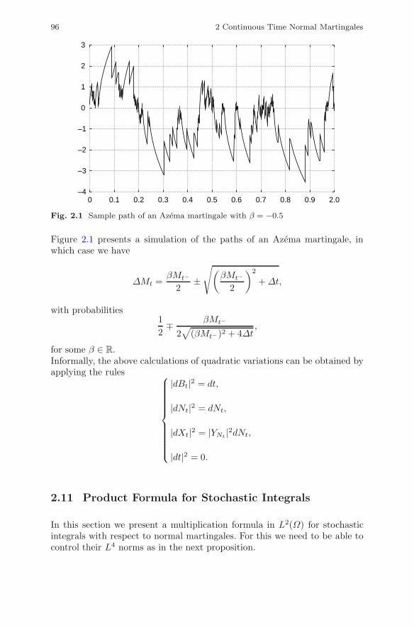
96 2 Continuous Time Normal Martingales
–4
–3
–2
–1
0
1
2
3
0 0.1 0.2 0.3 0.4 0.5 0.6 0.7 0.8 0.9 2.0
Fig. 2.1 Sample path of an Azema martingale with β = −0.5
Figure 2.1 presents a simulation of the paths of an Azema martingale, inwhich case we have
ΔMt =βMt−
2±√(
βMt−
2
)2
+Δt,
with probabilities12∓ βMt−
2√
(βMt−)2 + 4Δt,
for some β ∈ R.Informally, the above calculations of quadratic variations can be obtained byapplying the rules ⎧
⎪⎪⎪⎪⎪⎪⎪⎪⎪⎨
⎪⎪⎪⎪⎪⎪⎪⎪⎪⎩
|dBt|2 = dt,
|dNt|2 = dNt,
|dXt|2 = |YNt |2dNt,
|dt|2 = 0.
2.11 Product Formula for Stochastic Integrals
In this section we present a multiplication formula in L2(Ω) for stochasticintegrals with respect to normal martingales. For this we need to be able tocontrol their L4 norms as in the next proposition.
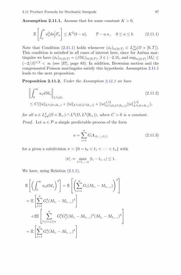
2.11 Product Formula for Stochastic Integrals 97
Assumption 2.11.1. Assume that for some constant K > 0,
E
[∫ b
a
φ2sds
∣∣∣Fa
]≤ K2(b− a), P − a.s., 0 ≤ a ≤ b. (2.11.1)
Note that Condition (2.11.1) holds whenever (φt)t∈[0,T ] ∈ L∞ad(Ω × [0, T ]).This condition is satisfied in all cases of interest here, since for Azema mar-tingales we have (φt)t∈[0,T ] = (βMt)t∈[0,T ], β ∈ (−2, 0), and supt∈[0,T ] |Mt| ≤(−2/β)1/2 < ∞ (see [37], page 83). In addition, Brownian motion and thecompensated Poisson martingales satisfy this hypothesis. Assumption 2.11.1leads to the next proposition.
Proposition 2.11.2. Under the Assumption 2.11.1 we have∥∥∥∥∫ ∞
0
usdMs
∥∥∥∥L4(Ω)
(2.11.2)
≤ C(‖u‖L4(Ω×R+) + ‖u‖L4(Ω,L2(R+)) + ‖u‖1/2L4(Ω,L2(R+))‖u‖1/2
L4(Ω×R+)),
for all u ∈ L4ad(Ω × R+) ∩ L4(Ω,L2(R+)), where C > 0 is a constant.
Proof. Let u ∈ P a simple predictable process of the form
u =n∑
i=1
Gi1(ti−1,ti], (2.11.3)
for a given a subdivision π = {0 = t0 < t1 < · · · < tn} with
|π| := maxi=1,...,n
|ti − ti−1| ≤ 1.
We have, using Relation (2.1.1),
E
[(∫ ∞
0
usdMs
)4]
= E
⎡
⎣(
n∑
i=1
Gi(Mti −Mti−1)
)4⎤
⎦
= E
[n∑
i=1
G4i (Mti −Mti−1)
4
]
+2E
⎡
⎣n∑
1≤i<j≤n
G2iG
2j(Mti −Mti−1)
2(Mtj −Mtj−1)2
⎤
⎦
= E
[n∑
i=1
G4i (Mti −Mti−1)
4
]

98 2 Continuous Time Normal Martingales
+2E
⎡
⎣n∑
1≤i<j≤n
G2iG
2j(Mti −Mti−1)
2(tj − tj−1)
⎤
⎦
≤ E
[n∑
i=1
G4i (Mti −Mti−1)
4
]
+2E
[n∑
i=1
G2i (Mti −Mti−1)
2
∫ ∞
ti
|us|2ds]
≤ E
[n∑
i=1
G4i (Mti −Mti−1)
4
]
+2
(E
[(∫ ∞
0
|us|2ds)2
])1/2⎛
⎝E
⎡
⎣(
n∑
i=1
G2i (Mti −Mti−1)
2
)2⎤
⎦
⎞
⎠1/2
.
We will deal successively with the three terms in the above expression. FromRelation (2.10.2) we have
E
[(n∑
i=1
G2i (Mti
− Mti−1 )2
)2](2.11.4)
= E
[(n∑
i=1
2G2i
∫ti
ti−1
(Mτ − Mti−1 )dMτ + G2i
∫ti
ti−1
φτdMτ + G2i (ti−1 − ti)
)2]
≤ 3E
[n∑
i=1
4G4i
(∫ ti
ti−1
(Mτ − Mti−1)dMτ
)2
+ G4i
(∫ ti
ti−1
φτdτ
)2
+ G4i (ti−1 − ti)
2
]
≤ 3E
[n∑
i=1
4G4i
∫ ti
ti−1
(Mτ − Mti−1)2dτ+G4
i (ti − ti−1)
∫ ti
ti−1
|φτ |2dτ+G4i (ti−1 − ti)
2
]
≤ 3E
[n∑
i=1
4G4i
∫ti
ti−1
(τ − ti−1)dτ + G4i (ti − ti−1)
∫ti
ti−1
|φτ |2dτ + G4i (ti−1 − ti)
2
]
≤ 3E
[n∑
i=1
G4i
(4
∫ti
ti−1
(τ − ti−1)dτ + (K2 + 1)(ti − ti−1)2)]
≤ 3(5 + K2)|π|‖u‖4L4(Ω×R+).
Next from Relation (2.10.2) we have
(Mt −Ms)4 = (t− s)(
2∫ t
s
(Mτ −Ms)dMτ +∫ t
s
φτdMτ + t− s
)
+2∫ t
s
(Mτ −Ms)dMτ
(2∫ t
s
(Mτ −Ms)dMτ +∫ t
s
φτdMτ + t− s
)
+∫ t
s
φτdMτ
(2∫ t
s
(Mτ −Ms)dMτ +∫ t
s
φτdMτ + t− s
),

2.11 Product Formula for Stochastic Integrals 99
hence from Proposition 2.5.7, Relations (2.1.1) and (2.5.4), and the condi-tional Ito isometry (2.5.4) we have
E[(Mt − Ms)4|Fs] = (t − s)2 + 4E
[∫ t
s
(Mτ − Ms)2dτ
∣∣∣Fs
]
+4E
[∫ t
s
φτ (Mτ − Ms)dτ∣∣∣Fs
]+ E
[∫ t
s
φ2τdτ
∣∣∣Fs
]
= (t − s)2 + 4
∫ t
s
(τ − s)2dτ
+4E
[∫ t
s
φτ (Mτ − Ms)dτ∣∣∣Fs
]+ E
[∫ t
s
φ2τdτ
∣∣∣Fs
]
≤ (t − s)2 + 4
∫ t
s
(τ − s)2dτ + E
[∫ t
s
φ2τdτ
∣∣∣Fs
]
+4
(E
[∫ t
s
φ2τdτ
∣∣∣Fs
])1/2 (E
[∫ t
s
(Mτ − Ms)2dτ
∣∣∣Fs
])1/2
≤ (t − s)2 + 4
∫ t
s
(τ − s)2dτ + E
[∫ t
s
φ2τdτ
∣∣∣Fs
]
+4
(E
[∫ t
s
φ2τdτ
∣∣∣Fs
])1/2 (∫ t
s
(τ − s)2dτ
)1/2
≤ (t − s)2 +4
3(t − s)3 +
4√3|t − s|3/2
(E
[∫ t
s
φ2τdτ
∣∣∣Fs
])1/2
+E
[∫ t
s
φ2τ dτ
∣∣∣Fs
]
≤ (t − s)
(K2 + t − s +
4K√3
(t − s) +4
3(t − s)2
),
which yields
E
[n∑
i=1
G4i (Mti −Mti−1)
4
]=
n∑
i=1
E[G4i E[(Mti −Mti−1)
4|Fti−1 ]]
≤(K2 + |π| + 4K√
3|π| + 4
3|π|2
)E
[n∑
i=1
G4i (ti − ti−1)
](2.11.5)
≤ K2‖u‖4L4(Ω×R+),
for some constant K > 0. Finally, ((2.11.4)) and (2.11.5) lead to (2.11.2).�
Next we state a multiplication formula for stochastic integrals with respectto a normal martingale.

100 2 Continuous Time Normal Martingales
Proposition 2.11.3. Under the Assumption 2.11.1, for all u ∈ L4ad(Ω ×
R+) ∩ L4(Ω,L2(R+)) we have∫ ∞
0
usdMs ∈ L4(Ω) and
(∫ ∞
0
usdMs
)2
= 2∫ ∞
0
us
∫ s
0
uτdMτdMs+∫ ∞
0
|us|2φsdMs+∫ ∞
0
|us|2ds.(2.11.6)
Proof. For simple predictable processes (us)s∈R+ of the form (2.11.3), for-mula (2.11.6) follows from (2.10.2). It is extended to u ∈ L4
ad(Ω × R+) ∩L4(Ω,L2(R+)) using (2.11.2) and the Ito isometry (2.5.4) which shows that
E
[(∫ ∞
0
|us|2φsdMs
)2]
= E
[n∑
i=1
|Gi|4∫ ti
ti−1
|φs|2ds]
≤ KE
[n∑
i=1
|Gi|4(ti − ti−1)
]
= K‖u‖4L4(Ω×R+),
and
E
[(∫ ∞
0
us
∫ s
0
uτdMτdMs
)2]
= E
[∫ ∞
0
|us|2(∫ s
0
uτdMτ
)2
ds
]
≤∫ ∞
0
E[|us|4
]1/2dsE
[(∫ s
0
uτdMτ
)4]1/2
≤ C‖u‖2L4(Ω×R+)(‖u‖2
L4(Ω×R+) + ‖u‖2L4(Ω,L2(R+))‖u‖2
L4(Ω×R+)),
for some constant C > 0. �The proof of Proposition 2.11.3 can easily be modified to show that we have
(∫ t
0
usdMs +∫ t
0
asds
)(∫ t
0
vsdMs +∫ t
0
bsds
)
=∫ t
0
us
∫ s
0
bτdτdMs +∫ t
0
bs
∫ s
0
uτdMτds
+∫ t
0
vs
∫ s
0
aτdτdMs +∫ t
0
as
∫ s
0
vτdMτds
+∫ t
0
as
∫ s
0
bτdτds+∫ t
0
bs
∫ s
0
aτdτds

2.11 Product Formula for Stochastic Integrals 101
+∫ t
0
us
∫ s
0
vτdMτdMs +∫ t
0
vs
∫ s
0
uτdMτdMs
+∫ t
0
φsusvsdMs +∫ t
0
usvsds, (2.11.7)
where all terms belong to L4(Ω), t ∈ R+, for all u, v, a, b ∈ L4ad(Ω × R+) ∩
L4(Ω,L2(R+)).As a corollary we have the following multiplication formula for multiplestochastic integrals.
Corollary 2.11.4. Let u∈L∞(R+) and v ∈L4(R+). Then under Assump-tion 2.11.1 we have for all n ≥ 1 and t ∈ R+:
I1(u1[0,t])In(1[0,t]nv⊗n)
=∫ t
0
usIn(1[0,s]nv⊗n)dMs + n
∫ t
0
vsIn−1(1[0,s]n−1v⊗(n−1))∫ s
0
uτdMτdMs
+n∫ t
0
φsusvsIn−1(1[0,s]n−1v⊗(n−1))dMs+n∫ t
0
usvsIn−1(1[0,s]n−1v⊗(n−1))ds.
Proof. Applying Proposition 2.11.3 to us and vsIn−1(1[0,s]n−1v⊗(n−1)), wehave
I1(u1[0,t])In(1[0,t]nv⊗n) = n
∫ t
0
usdMs
∫ t
0
vsIn−1(1[0,s]n−1v⊗(n−1))dMs
= n
∫ t
0
us
∫ s
0
vτ In−1(1[0,τ ]n−1v⊗(n−1))dMτdMs
+n∫ t
0
vsIn−1(1[0,s]n−1v⊗(n−1))∫ s
0
uτdMτdMs
+n∫ t
0
φsusvsIn−1(1[0,s]n−1v⊗(n−1))dMs
+n∫ t
0
usvsIn−1(1[0,s]n−1v⊗(n−1))ds
=∫ t
0
usIn(1[0,s]nv⊗n)dMs + n
∫ t
0
vsIn−1(1[0,s]n−1v⊗(n−1))∫ s
0
uτdMτdMs
+n∫ t
0
φsusvsIn−1(1[0,s]n−1v⊗(n−1))dMs
+n∫ t
0
usvsIn−1(1[0,s]n−1v⊗(n−1))ds.
�
102 2 Continuous Time Normal Martingales
2.12 Ito Formula
Consider a normal martingale (Mt)t∈R+ satisfying the structure equation
d[M,M ]t = dt+ φtdMt.
Such an equation is satisfied in particular if (Mt)t∈R+ has the predictablerepresentation property, cf. Proposition 2.10.2.The following is a statement of Ito’s formula for normal martingales, cf. [37],page 70, for a proof using formal semimartingales. The proof presented hereis in the L2 sense.
Proposition 2.12.1. Assume that φ ∈ L∞ad([0, T ]× Ω). Let (Xt)t∈[0,T ] be aprocess given by
Xt = X0 +∫ t
0
usdMs +∫ t
0
vsds, t ∈ [0, T ], (2.12.1)
where (us)s∈[0,T ] and (vs)s∈[0,T ] are adapted processes in L2ad(Ω × [0, T ]).
Then for all f ∈ C1,2(R+ × R) we have
f(t,Xt) − f(0, X0) =∫ t
0
f(s,Xs− + φsus) − f(s,Xs−)φs
dMs (2.12.2)
+∫ t
0
f(s,Xs + φsus) − f(s,Xs) − φsus∂f
∂x(s,Xs)
φ2s
ds
+∫ t
0
vs∂f
∂x(s,Xs)ds+
∫ t
0
∂f
∂s(s,Xs)ds, t ∈ [0, T ].
Proof. We prove the formula in the case where f does not depend on timeand vs = 0, s ∈ R+, since this generalization can be done using standardcalculus arguments. Assume now that u ∈ U is a simple predictable processof the form u = G1[a,b], with G ∈ L∞(Ω,Fa). Clearly the formula (2.12.2)holds when f = c is a constant function. By induction on n ≥ 1, we assumethat it holds when applied to f(x) = xn, i.e.
Xnt = Xn
0 +∫ t
0
Lns ds+
∫ t
0
Uns dMs,
with
Uns =
(Xs− + φsus)n − (Xs−)n
φs,

2.12 Ito Formula 103
and
Lns =
(Xs + φsus)n − (Xs)n − nφsus(Xs)n−1
φ2s
, s ∈ R+.
From Proposition 2.11.3 we have
Xn+1t −Xn
0 = (Xt −X0)(Xnt −Xn
0 ) +X0(Xnt −Xn
0 ) +Xn0 (Xt −X0)
=∫ t
0
us
∫ s
0
Lnτ dτdM s +
∫ t
0
us
∫ s
0
Unτ dMτdMs
+∫ t
0
Lns
∫ s
0
uτdMτds+∫ t
0
Uns
∫ s
0
uτdMτdMs
+∫ t
0
φsusUns dMs +
∫ t
0
usUns ds
+X0
∫ t
0
Lns ds+X0
∫ t
0
Uns dMs,+Xn
0
∫ t
0
usdMs
=∫ t
0
XsUns dMs +
∫ t
0
XsLnsds+
∫ t
0
Xns usdMs
+∫ t
0
usφsUns dMs +
∫ t
0
usUns ds
=∫ t
0
Ln+1s ds+
∫ t
0
Un+1s dMs,
since
Un+1s = us(Xs−)n +Xs−Un
s + usφsUns = usX
ns− +Xs−Un
s + usφsUns ,
andLn+1
s = Uns us +Xs−Ln
s , s ∈ R+, n ∈ N.
This proves the formula for f polynomial and u ∈ P . For all n ≥ 1, let
τn = inf{s ∈ R+ : |Xs| > n}.
Let f ∈ C2b (R) and let (fm)m∈N be a sequence of polynomials converging
uniformly to f on [−n, n]. Since 1{s≤τn} = 1, a.s., 0 ≤ s ≤ t, on {t ≤ τn},from the locality property of the stochastic integral (Proposition 2.5.5) wehave for all m ∈ N:
1{t≤τn}(fm(Xt) − fm(X0)) = 1{t≤τn}
∫ t
0
fm(Xs− + φsus) − fm(Xs−)φs
dMs
+1{t≤τn}
∫ t
0
fm(Xs− + φsus) − fm(Xs−) − φsusf′m(Xs−)
φ2s
ds

104 2 Continuous Time Normal Martingales
= 1{t≤τn}
∫ t
0
1{s≤τn}fm(Xs− + φsus) − fm(Xs−)
φsdMs
+1{t≤τn}
∫ t
0
1{s≤τn}fm(Xs− + φsus) − fm(Xs−) − φsusf
′m(Xs−)
φ2s
ds.
Letting m go to infinity we get
1{t≤τn}(f(Xt) − f(X0))
= 1{t≤τn}
∫ t
0
1{s≤τn}f(Xs− + φsus) − f(Xs−)
φsdMs
+1{t≤τn}
∫ t
0
1{s≤τn}f(Xs− + φsus) − f(Xs−) − φsusf
′(Xs−)φ2
s
ds,
and it remains to let n go to infinity, which proves the formula for f ∈ C2b (R)
by locality of the Ito integral. The formula is then extended to u ∈ L2ad([0, T ]×
Ω), by density of U in L2ad([0, T ]×Ω), and finally to all f ∈ C2(R), again by
locality of the Ito integral. �Note that if φs = 0, the terms
f(Xs− + φsus) − f(Xs−)φs
andf(Xs + φsus) − f(Xs) − φsusf
′(Xs)φ2
s
have to be replaced by their respective limits usf′(Xs−) and 1
2u2sf′′(Xs−) as
φs → 0. This gives
f(t,Xt) − f(0, X0) =∫ t
0
isus∂f
∂x(s,Xs)dMs +
12
∫ t
0
isu2s
∂2f
∂x2(s,Xs)ds
+∫ t
0
jsf(s,Xs− + φsus) − f(s,Xs−)
φsdMs
+∫ t
0
jsf(s,Xs + φsus) − f(s,Xs) − φsus
∂f
∂x(s,Xs)
φ2s
ds
+∫ t
0
vs∂f
∂x(s,Xs)ds+
∫ t
0
∂f
∂s(s,Xs)ds, t ∈ [0, T ],
where the processes (it)t∈R+ and (jt)t∈R+ have been defined in (2.10.3).
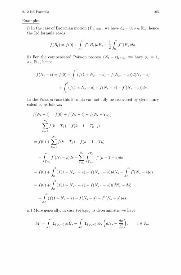
2.12 Ito Formula 105
Examples
i) In the case of Brownian motion (Bt)t∈R+ we have φs = 0, s ∈ R+, hencethe Ito formula reads
f(Bt) = f(0) +∫ t
0
f ′(Bs)dBs +12
∫ t
0
f ′′(Bs)ds.
ii) For the compensated Poisson process (Nt − t)t∈R+ we have φs = 1,s ∈ R+, hence
f(Nt − t) = f(0) +∫ t
0
(f(1 +Ns− − s) − f(Ns− − s))d(Ns − s)
+∫ t
0
(f(1 +Ns − s) − f(Ns − s) − f ′(Ns − s))ds.
In the Poisson case this formula can actually be recovered by elementarycalculus, as follows:
f(Nt − t) = f(0) + f(Nt − t) − f(Nt − TNt)
+Nt∑
k=1
f(k − Tk) − f(k − 1 − Tk−1)
= f(0) +Nt∑
k=1
f(k − Tk) − f(k − 1 − Tk)
−∫ t
TNt
f ′(Nt − s)ds−Nt∑
k=1
∫ Tk
Tk−1
f ′(k − 1 − s)ds
= f(0) +∫ t
0
(f(1 +Ns− − s) − f(Ns− − s))dNs −∫ t
0
f ′(Ns − s)ds
= f(0) +∫ t
0
(f(1 +Ns− − s) − f(Ns− − s))(dNs − ds)
+∫ t
0
(f(1 +Ns − s) − f(Ns − s) − f ′(Ns − s))ds.
iii) More generally, in case (φt)t∈R+ is deterministic we have
Mt =∫ t
0
1{φs=0}dBs +∫ t
0
1{φs �=0}φs
(dNs − ds
φ2s
), t ∈ R+,

106 2 Continuous Time Normal Martingales
and
f(Mt) = f(0) +∫ t
0
1{φs=0}f ′(Ms)dBs +12
∫ t
0
1{φs=0}f ′′(Ms)dBs
+∫ t
0
1{φs �=0}(f(Ms− + φs) − f(Ms−))(dNs − ds
φ2s
)
+∫ t
0
1{φs �=0}(f(Ms− + φs) − f(Ms−) − φsf′(Ms))
ds
φ2s
.
iv) For the compound Poisson martingale
Mt :=Xt − λtE[Y1]√
λVar [Y1], t ∈ R+,
of Section 2.4 we have
f(Mt) = f(0) +∫ t
0
(f(YNs +Ms−) − f(Ms−))d(Ns − λs) (2.12.3)
+λ∫ t
0
(f(YNs +Ms) − f(Ms) − E[Y1]√
λVar [Y1]f ′(Ms)
)ds.
However, as noted above the compound Poisson martingale (2.10.5) doesnot have the predictable representation property. Thus it does not satisfythe hypotheses of this section and the above formula is actually distinctfrom (2.12.1) since here the stochastic integral is not with respect to(Mt)t∈R+ itself. Note also that the pathwise stochastic integral (2.12.3)is not in the sense of Proposition 2.5.10 since the integrand (f(YNt +Mt−) − f(Mt−)) is not a left limit due to the presence of YNt .
The change of variable formula can be extended to the multidimensional caseas in Proposition 2 of [37]. Here we use the convention 0/0 = 0.Proposition 2.12.2. Let X = (Xt)t∈R+ be a R
n-valued process given by
dXt = Rtdt+KtdMt, X0 > 0,
where (Rt)t∈R+ and (Kt)t∈R+ are predictable square-integrable Rn-valued pro-
cesses. For any f ∈ C2b (R+ × R
n; R) we have
f(t,Xt) = f(0, X0)+∫ t
0
Lsf(s,Xs)dMs+∫ t
0
Usf(s,Xs)ds+∫ t
0
∂f
∂s(s,Xs)ds,
(2.12.4)where
Lsf(s,Xs) = is〈Ks,∇f(s,Xs)〉 +jsφs
(f(s,Xs− + φsKs−) − f(s,Xs−)),
(2.12.5)

2.13 Exponential Vectors 107
and
Usf(s,Xs) = Rs∇f(s,Xs) + α2s
(12is〈Hess f(s,Xs),Ks ⊗Ks〉
+jsφ2
s
(f(s,Xs− + φsKs−) − f(s,Xs−) − φs〈Ks,∇f(s,Xs)〉)).
2.13 Exponential Vectors
The exponential vectors are a stochastic analog of the generating functionfor polynomials. In this section they are presented as the solutions of lin-ear stochastic differential equations with respect to a normal martingale(Mt)t∈R+ having the predictable representation property, and satisfying astructure equation of the form (2.10.1).In the next proposition, the solution (2.13.2) of Equation 2.13.1 can be de-rived using the Ito formula, and the uniqueness can be proved using the Itoisometry and classical arguments.
Proposition 2.13.1. For any u ∈ L2ad(Ω × R+), the equation
Zt = 1 +∫ t
0
Zs−usdMs, t ∈ [0, T ] (2.13.1)
has a unique solution (ξt(u))t∈R+ given by
ξt(u) = exp(∫ t
0
usdMs − 12
∫ t
0
u2s1{φs=0}ds
) ∏
s∈JtM
(1 + usφs)e−usφs ,
(2.13.2)
where J tM denotes the set of jump times of (Ms)s∈[0,t], t ∈ [0, T ].
In the pure jump case, from Proposition 2.5.10, (Zs)s∈R+ satisfies the path-wise stochastic differential equation with jumps
dGt = u(t)Gt−(dNt − dt), G0 = 1, (2.13.3)
which can be directly solved on each interval (Tk−1, Tk], k ≥ 1, to get
Gt = e−∫
t0 u(s)ds
Nt∏
k=1
(1 + u(Tk)), t ∈ R+.
Proposition 2.13.2. Given u ∈ L∞([0, T ]), ξT (u) can be represented as
ξT (u) =∞∑
n=0
1n!In(u⊗n1[0,T ]n). (2.13.4)
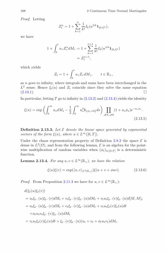
108 2 Continuous Time Normal Martingales
Proof. Letting
Znt = 1 +
n∑
k=1
1k!Ik(u⊗k1[0,t]k),
we have
1 +∫ t
0
uτZnτ dMτ = 1 +
n+1∑
k=1
1k!Ik(u⊗k1[0,t]k)
= Zn+1t ,
which yields
Zt = 1 +∫ t
0
uτZτdMτ , t ∈ R+,
as n goes to infinity, where integrals and sums have been interchanged in theL2 sense. Hence ξt(u) and Zt coincide since they solve the same equation(2.13.1). �In particular, letting T go to infinity in (2.13.2) and (2.13.4) yields the identity
ξ(u) = exp(∫ ∞
0
usdMs − 12
∫ ∞
0
u2s1{φs=0}ds
) ∏
ΔNs �=0
(1 + usφs)e−usφs .
(2.13.5)
Definition 2.13.3. Let E denote the linear space generated by exponentialvectors of the form ξ(u), where u ∈ L∞([0, T ]).
Under the chaos representation property of Definition 2.8.2 the space E isdense in L2(Ω), and from the following lemma, E is an algebra for the point-wise multiplication of random variables when (φt)t∈[0,T ] is a deterministicfunction.
Lemma 2.13.4. For any u, v ∈ L∞(R+), we have the relation
ξ(u)ξ(v) = exp(〈u, v〉L2(R+))ξ(u + v + φuv). (2.13.6)
Proof. From Proposition 2.11.3 we have for u, v ∈ L∞(R+):
d(ξt(u)ξt(v))
= utξt−(u)ξt−(v)dMt + vtξt−(v)ξt−(u)dMt + vtutξt−(v)ξt−(u)d[M,M ]t
= utξt−(u)ξt−(v)dMt + vtξt−(v)ξt−(u)dMt + vtutξt(v)ξt(u)dt
+φtutvtξt−(v)ξt−(u)dMt
= vtutξt(v)ξt(u)dt+ ξt−(v)ξt−(u)(ut + vt + φtutvt)dMt.
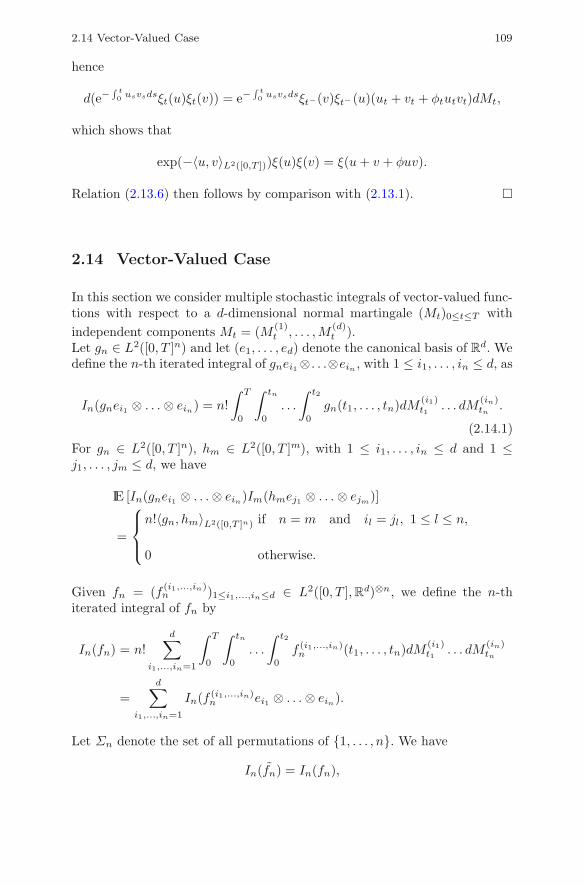
2.14 Vector-Valued Case 109
hence
d(e−∫ t0 usvsdsξt(u)ξt(v)) = e−
∫ t0 usvsdsξt−(v)ξt− (u)(ut + vt + φtutvt)dMt,
which shows that
exp(−〈u, v〉L2([0,T ]))ξ(u)ξ(v) = ξ(u+ v + φuv).
Relation (2.13.6) then follows by comparison with (2.13.1). �
2.14 Vector-Valued Case
In this section we consider multiple stochastic integrals of vector-valued func-tions with respect to a d-dimensional normal martingale (Mt)0≤t≤T withindependent components Mt = (M (1)
t , . . . ,M(d)t ).
Let gn ∈ L2([0, T ]n) and let (e1, . . . , ed) denote the canonical basis of Rd. We
define the n-th iterated integral of gnei1 ⊗ . . .⊗ein , with 1 ≤ i1, . . . , in ≤ d, as
In(gnei1 ⊗ . . .⊗ ein) = n!∫ T
0
∫ tn
0
. . .
∫ t2
0
gn(t1, . . . , tn)dM (i1)t1 . . . dM
(in)tn
.
(2.14.1)For gn ∈ L2([0, T ]n), hm ∈ L2([0, T ]m), with 1 ≤ i1, . . . , in ≤ d and 1 ≤j1, . . . , jm ≤ d, we have
IE [In(gnei1 ⊗ . . .⊗ ein)Im(hmej1 ⊗ . . .⊗ ejm)]
=
⎧⎪⎨
⎪⎩
n!〈gn, hm〉L2([0,T ]n) if n = m and il = jl, 1 ≤ l ≤ n,
0 otherwise.
Given fn = (f (i1,...,in)n )1≤i1,...,in≤d ∈ L2([0, T ],Rd)⊗n, we define the n-th
iterated integral of fn by
In(fn) = n!d∑
i1,...,in=1
∫ T
0
∫ tn
0
. . .
∫ t2
0
f (i1,...,in)n (t1, . . . , tn)dM (i1)
t1 . . . dM(in)tn
=d∑
i1,...,in=1
In(f (i1,...,in)n ei1 ⊗ . . .⊗ ein).
Let Σn denote the set of all permutations of {1, . . . , n}. We have
In(fn) = In(fn),
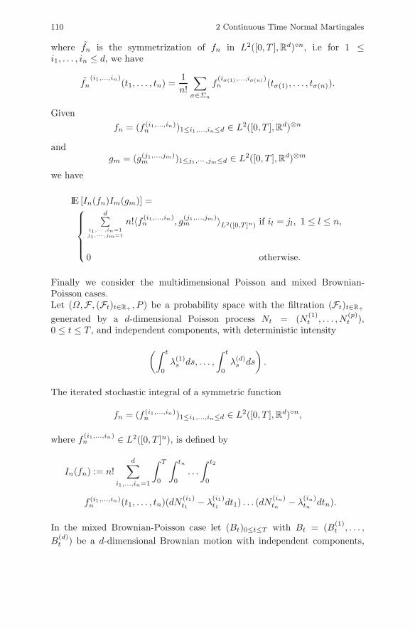
110 2 Continuous Time Normal Martingales
where fn is the symmetrization of fn in L2([0, T ],Rd)◦n, i.e for 1 ≤i1, . . . , in ≤ d, we have
fn(i1,...,in)
(t1, . . . , tn) =1n!
∑
σ∈Σn
f(iσ(1),...,iσ(n))n (tσ(1), . . . , tσ(n)).
Givenfn = (f (i1,...,in)
n )1≤i1,...,in≤d ∈ L2([0, T ],Rd)⊗n
andgm = (g(j1,...,jm)
m )1≤j1,··· ,jm≤d ∈ L2([0, T ],Rd)⊗m
we have
IE [In(fn)Im(gm)] =⎧⎪⎪⎪⎨
⎪⎪⎪⎩
d∑i1,··· ,in=1j1,··· ,jm=1
n!〈f (i1,...,in)n , g
(j1,...,jm)m 〉L2([0,T ]n) if il = jl, 1 ≤ l ≤ n,
0 otherwise.
Finally we consider the multidimensional Poisson and mixed Brownian-Poisson cases.Let (Ω,F , (Ft)t∈R+ , P ) be a probability space with the filtration (Ft)t∈R+
generated by a d-dimensional Poisson process Nt = (N (1)t , . . . , N
(p)t ),
0 ≤ t ≤ T , and independent components, with deterministic intensity
(∫ t
0
λ(1)s ds, . . . ,
∫ t
0
λ(d)s ds
).
The iterated stochastic integral of a symmetric function
fn = (f (i1,...,in)n )1≤i1,...,in≤d ∈ L2([0, T ],Rd)◦n,
where f (i1,...,in)n ∈ L2([0, T ]n), is defined by
In(fn) := n!d∑
i1,...,in=1
∫ T
0
∫ tn
0
. . .
∫ t2
0
f (i1,...,in)n (t1, . . . , tn)(dN (i1)
t1 − λ(i1)t1 dt1) . . . (dN
(in)tn
− λ(in)tn
dtn).
In the mixed Brownian-Poisson case let (Bt)0≤t≤T with Bt = (B(1)t , . . . ,
B(d)t ) be a d-dimensional Brownian motion with independent components,

2.15 Notes and References 111
let (Nt)0≤t≤T with Nt = (N (1)t , . . . , N
(p)t ) be a p-dimensional Poisson process
with independent components and intensity
(∫ t
0
λ(1)s ds, . . . ,
∫ t
0
λ(d)s ds
).
We work on a filtered probability space (Ω,F , (Ft)t∈[0,T ], P ), where Ft isthe filtration generated by (Bt)t∈R+ and (Nt)t∈R+ , which are assumed to beindependent. We denote by M = (M (1), . . . ,M (p)) the compensated Poissonprocess given by
dM (l) = dN(l)t − λ
(l)t dt, t ∈ [0, T ], l = 1, . . . , p.
Let
(X(1)t , . . . , X
(d)t , X
(d+1)t , . . . , X
(d+p)t ) = (B(1)
t , . . . , B(d)t ,M
(1)t , . . . ,M
(p)t ).
The iterated stochastic integral of a symmetric function
fn = (f (i1,...,in)n )1≤i1,...,in≤d+p ∈ L2([0, T ],R(d+p))⊗n,
where f (i1,...,in)n ∈ L2([0, T ]n), is given by
In(fn) := n!d+p∑
i1,...,in=1
∫ T
0
∫ tn
0
. . .
∫ t2
0
f (i1,...,in)n (t1, . . . , tn)dX(i1)
t1 . . . dX(in)tn
.
The chaos representation property holds in the multidimensional case, i.e.for any F ∈ L2(Ω) there exists a unique sequence (fn)n∈N of symmetricdeterministic functions
fn = (f (i1,...,in)n )i1,...,in∈{1,...,d} ∈ L2([0, T ],Rd)◦n
such that
F =∞∑
n=0
In(fn).
2.15 Notes and References
Our presentation of stochastic calculus is restricted to normal martingales,which are well fitted to the construction of multiple stochastic integrals andchaos expansions in the L2 sense. We refer to e.g. [121] for the the standardapproach to stochastic calculus using local martingales and semimartingales.

112 2 Continuous Time Normal Martingales
The systematic study of normal martingales started in [37], and d-dimensionalnormal martingales have been considered in [9], [10]. Several books and sur-veys exist on multiple stochastic integrals, see [39], [58], [73], [82]. A numberof properties of Brownian motion, such as almost sure path continuity, havebeen omitted here and can be found in [122]. See [26], page 317, and [24], [153]for the absence of predictable representation property of compound Poissonprocesses. The Ito change of variable formula Proposition 2.12.1 can be foundin Proposition 2 in [37] with a different formulation and proof. We refer to[121], Theorem 36, page 77, for results on exponential vectors. Lemma 2.13.4is a version of Yor’s formula [152], cf. also Theorem 37 of [119], page 79,for martingales with deterministic bracket 〈M,M〉t. Proposition 2.3.6 canbe proved using the independence of increments of the Poisson process andarguments of [87]. The presentation of multidimensional Poisson and mixedBrownian-Poisson integrals is based on [69].
Chapter 3
Gradient and Divergence Operators
In this chapter we construct an abstract framework for stochastic analysisin continuous time with respect to a normal martingale (Mt)t∈R+ , using theconstruction of stochastic calculus presented in Section 2. In particular weidentify some minimal properties that should be satisfied in order to connecta gradient and a divergence operator to stochastic integration, and to applythem to the predictable representation of random variables. Some applica-tions, such as logarithmic Sobolev and deviation inequalities, are formulatedin this general setting. In the next chapters we will examine concrete exam-ples of operators that can be included in this framework, in particular when(Mt)t∈R+ is a Brownian motion or a compensated Poisson process.
3.1 Definition and Closability
In this chapter, (Mt)t∈R+ denotes a normal martingale as considered inChapter 2. We let S, U , and P denote the spaces of random variables, simpleprocesses and simple predictable processes introduced in Definition 2.5.2, andwe note that S is dense in L2(Ω) by Definition 2.5.2 and U , P are dense inL2(Ω × R+) respectively from Proposition 2.5.3.Let now
D : L2(Ω, dP) → L2(Ω × R+, dP × dt)
andδ : L2(Ω × R+, dP × dt) → L2(Ω, dP)
be linear operators defined respectively on S and U . We assume that thefollowing duality relation holds.
Assumption 3.1.1. (Duality relation) The operators D and δ satisfy therelation
IE[〈DF, u〉L2(R+)] = IE[Fδ(u)], F ∈ S, u ∈ U . (3.1.1)
Note that D1 = 0 is equivalent to IE[δ(u)] = 0, for all u ∈ U . In the nextproposition we use the notion of closability for operators in normed linear
N. Privault, Stochastic Analysis in Discrete and Continuous Settings,Lecture Notes in Mathematics 1982, DOI 10.1007/978-3-642-02380-4 3,c© Springer-Verlag Berlin Heidelberg 2009
113

114 3 Gradient and Divergence Operators
spaces, whose definition is recalled in Section 9.8 of the Appendix. The nextproposition is actually a general result on the closability of the adjoint of adensely defined operator.
Proposition 3.1.2. The duality assumption 3.1.1 implies that D and δ areclosable.
Proof. If (Fn)n∈N converges to 0 in L2(Ω) and (DFn)n∈N converges to U ∈L2(Ω × R+), the relation
IE[〈DFn, u〉L2(R+)] = IE[Fnδ(u)], u ∈ U ,
implies
| IE[〈U, u〉L2(R+)]|≤ | IE[〈DFn, u〉L2(R+)] − IE[〈U, u〉L2(R+)]| + | IE[〈DFn, u〉L2(R+)|= | IE[〈DFn − U, u〉L2(R+)]| + | IE[Fnδ(u)]|≤ ‖DFn − U‖L2(Ω×R+)‖u‖L2(Ω×R+) + ‖Fn‖L2(Ω)‖δ(u)‖L2(Ω),
hence as n goes to infinity we get IE[〈U, u〉L2(R+)] = 0, u ∈ U , i.e. U = 0 sinceU is dense in L2(Ω × R+). The proof of closability of δ is similar: if (un)n∈N
converges to 0 in L2(Ω × R+) and (δ(un))n∈N converges to F ∈ L2(Ω), wehave for all G ∈ S:
| IE[FG]| ≤ | IE[〈DG, un〉L2(R+)] − IE[FG]| + | IE[〈DG, un〉L2(R+)]|= | IE[G(δ(un) − F )]| + | IE[〈DG, un〉L2(Ω×R+)]|≤ ‖δ(un) − F‖L2(Ω)‖G‖L2(Ω) + ‖un‖L2(Ω×R+)‖DG‖L2(Ω×R+),
hence IE[FG] = 0, G ∈ S, i.e. F = 0 since S is dense in L2(Ω). �From the above proposition these operators are respectively extended to theirclosed domains Dom (D) and Dom (δ), and for simplicity their extensions willremain denoted by D and δ.
3.2 Clark Formula and Predictable Representation
In this section we study the connection between D, δ, and the predictablerepresentation of random variables using stochastic integrals.
Assumption 3.2.1. (Clark formula). Every F ∈ S can be represented as
F = IE[F ] +∫ ∞
0
IE[DtF |Ft]dMt. (3.2.1)
3.2 Clark Formula and Predictable Representation 115
This assumption is connected to the predictable representation propertyfor the martingale (Mt)t∈R+ , cf. Proposition 3.2.8 and Proposition 3.2.6below.
Definition 3.2.2. Given k ≥ 1, let ID2,k([a,∞)), a > 0, denote the comple-tion of S under the norm
‖F‖ID2,k([a,∞)) = ‖F‖L2(Ω) +k∑
i=1
(∫ ∞
a
|DitF |2dt
)1/2
,
where Dit = Dt · · ·Dt denotes the i-th iterated power of Dt, i ≥ 1.
In other words, for any F ∈ ID2,k([a,∞)), the process (DtF )t∈[a,∞) exists inL2(Ω × [a,∞)). Clearly we have Dom (D) = ID2,1([0,∞)). Under the Clarkformula Assumption 3.2.1, a representation result for F ∈ ID2,1([a,∞)) canbe stated as a consequence of the Clark formula:
Proposition 3.2.3. For all t ∈ R+ > 0 and F ∈ ID2,1([t,∞)) we have
IE[F |Ft] = IE[F ] +∫ t
0
IE[DsF |Fs]dMs, (3.2.2)
andF = IE[F |Ft] +
∫ ∞
t
IE[DsF |Fs]dMs, t ∈ R+. (3.2.3)
Proof. This is a direct consequence of (3.2.1) and Proposition 2.5.7. �By uniqueness of the predictable representation of F ∈ L2(Ω), an expressionof the form
F = c+∫ ∞
0
utdMt
where c ∈ R and (ut)t∈R+ is adapted and square-integrable, implies
ut = E[DtF |Ft], dt× dP − a.e.
The covariance identity proved in the next lemma is a consequence ofProposition 3.2.3 and the Ito isometry (2.5.5).
Lemma 3.2.4. For all t ∈ R+ and F ∈ ID2,1([t,∞)) we have
IE[(IE[F |Ft])2] = (IE[F ])2 + IE[∫ t
0
(IE[DsF |Fs])2ds]
(3.2.4)
= IE[F 2] − IE[∫ ∞
t
(IE[DsF |Fs])2ds]. (3.2.5)

116 3 Gradient and Divergence Operators
Proof. From the Ito isometry (2.5.4) and Relation 3.2.2 we have
IE[(IE[F |Ft])2] = IE
[(IE[F ] +
∫ t
0
IE[DsF |Fs]dMs
)2]
= (IE[F ])2 + IE
[(∫ t
0
IE[DsF |Fs]dMs
)2]
= (IE[F ])2 + IE[∫ t
0
(IE[DsF |Fs])2ds], t ∈ R+,
which shows (3.2.4). Next, concerning (3.2.5) we have
IE[F 2] = IE
[(IE[F |Ft] +
∫ ∞
t
IE[DsF |Fs]dMs
)2]
= IE[(IE[F |Ft])
2]
+ IE[IE[F |Ft]
∫ ∞
t
IE[DsF |Fs]dMs
]
+ IE
[(∫ ∞
t
IE[DsF |Fs]dMs
)2]
= IE[(IE[F |Ft])
2]
+ IE[∫ ∞
t
IE[F |Ft] IE[DsF |Fs]dMs
]
+ IE[∫ ∞
t
(IE[DsF |Fs])2ds
]
= IE[(IE[F |Ft])
2]
+ IE[∫ ∞
t
(IE[DsF |Fs])2ds
], t ∈ R+,
since from (2.5.7) the Ito stochastic integral has expectation 0, which shows(3.2.5). �The next remark applies in general to any mapping sending a random variableto the process involved in its predictable representation with respect to anormal martingale.Lemma 3.2.5. The operator
F → (IE[DtF |Ft])t∈R+
defined on S extends to a continuous operator from L2(Ω) into L2(Ω×R+).
Proof. This follows from the bound
‖ IE[D·F |F·]‖2L2(Ω×R+) = ‖F‖2
L2(Ω) − (IE[F ])2
≤ ‖F‖2L2(Ω),
that follows from Relation (3.2.4) with t = 0. �

3.2 Clark Formula and Predictable Representation 117
As a consequence of Lemma 3.2.5, the Clark formula can be extended inProposition 3.2.6 below as in the discrete case, cf. Proposition 1.7.2.
Proposition 3.2.6. The Clark formula
F = IE[F ] +∫ ∞
0
IE[DtF |Ft]dMt.
can be extended to all F in L2(Ω).
Similarly, the results of Proposition 3.2.3 and Lemma 3.2.4 also extend toF ∈ L2(Ω).The Clark representation formula naturally implies a Poincare typeinequality.
Proposition 3.2.7. For all F ∈ Dom (D) we have
Var (F ) ≤ ‖DF‖2L2(Ω×R+).
Proof. From Lemma 3.2.4 we have
Var (F ) = IE[|F − E[F ]|2]
= IE
[(∫ ∞
0
IE[DtF |Ft]dMt
)2]
= IE[∫ ∞
0
(IE[DtF |Ft])2dt
]
≤ IE[∫ ∞
0
IE[|DtF |2|Ft]dt]
≤∫ ∞
0
IE[IE[|DtF |2|Ft]
]dt
≤∫ ∞
0
IE[|DtF |2
]dt
≤ IE[∫ ∞
0
|DtF |2dt],
hence the conclusion. �Since the space S is dense in L2(Ω) by Definition 2.5.2, the Clark for-mula Assumption 3.2.1 implies the predictable representation property ofDefinition 2.6.1 for (Mt)t∈R+ as a consequence of the next corollary.
Corollary 3.2.8. Under the Clark formula Assumption 3.2.1 the martingale(Mt)t∈R+ has the predictable representation property.
Proof. Definition 2.6.1 is satisfied because S is dense in L2(Ω) and the process(IE[DtF | Ft])t∈R+ in (3.2.1) can be approximated by a sequence in P fromProposition 2.5.3.

118 3 Gradient and Divergence Operators
Alternatively, one may use Proposition 2.6.2 and proceed as follows. Considera square-integrable martingale (Xt)t∈R+ with respect to (Ft)t∈R+ and let
us = IE[DsXn+1|Fn], n ≤ s < n+ 1, t ∈ R+.
Then (ut)t∈R+ is an adapted process such that u1[0,T ] ∈ L2(Ω × R+) for allT > 0, and the Clark formula Assumption 3.2.1 and Proposition 3.2.6 imply
Xt = IE[Xn+1 | Ft]
= IE[X0 +
∫ n+1
0
IE[DsXn+1 | Fs]dMs
∣∣∣Ft
]
= X0 +∫ t
0
IE [DsXn+1 | Fs] dMs
= X0 +∫ n
0
IE [DsXn+1 | Fs] dMs +∫ t
n
IE [DsXn+1 | Fs] dMs
= Xn +∫ t
n
IE[DsXn+1 | Fs]dMs
= Xn +∫ t
n
usdMs, n ≤ t < n+ 1, n ∈ N,
where we used the Chasles relation (2.5.6), hence
Xt = X0 +∫ t
0
usdMs, t ∈ R+, (3.2.6)
hence from Proposition 2.6.2, (Mt)t∈R+ has the predictable representationproperty. �In particular, the Clark formula Assumption 3.2.1 and Relation (3.2.3) ofProposition 3.2.3 imply the following proposition.
Proposition 3.2.9. For any FT -measurable F ∈ L2(Ω) we have
IE[DtF |FT ] = 0, 0 ≤ T ≤ t. (3.2.7)
Proof. From from Relation (3.2.3) we have F = IE[F |FT ] if and only if
∫ ∞
T
IE[DtF |Ft]dMt = 0,
which implies IE[DtF |Ft], t ≥ T , by the Ito isometry (2.5.4), hence (3.2.7)holds as
IE[DtF |FT ] = IE[IE[DtF |Ft]|FT ] = 0, t ≥ T,
by the tower property of conditional expectations stated in Section 9.3. �

3.3 Divergence and Stochastic Integrals 119
The next assumption is a stability property for the gradient operator D.
Assumption 3.2.10. (Stability property) For all FT -measurable F ∈ S,DtF is FT -measurable for all t ≥ T .
Proposition 3.2.11. Let T > 0. Under the stability Assumption 3.2.10, forany FT -measurable random variable F ∈ L2(Ω) we have F ∈ ID[T,∞) and
DtF = 0, t ≥ T.
Proof. Since F is FT -measurable, DtF is FT -measurable, t ≥ T , by thestability Assumption 3.2.10, and from Proposition 3.2.9 we have
DtF = IE[DtF |FT ] = 0, 0 ≤ T ≤ t.
�
3.3 Divergence and Stochastic Integrals
In this section we are interested in the connection between the operator δand the stochastic integral with respect to (Mt)t∈R+ .
Proposition 3.3.1. Under the duality Assumption 3.1.1 and the Clark for-mula Assumption 3.2.1, the operator δ applied to any square-integrableadapted process (ut)t∈R+ ∈ L2
ad(Ω × R+) coincides with the stochastic in-tegral
δ(u) =∫ ∞
0
utdMt, u ∈ L2ad(Ω × R+), (3.3.1)
of (ut)t∈R+ with respect to (Mt)t∈R+ , and the domain Dom (δ) of δ containsL2
ad(Ω × R+).
Proof. Let u ∈ P be a simple Ft-predictable process. From the dualityAssumption 3.1.1 and the fact (2.5.7) that
IE[∫ ∞
0
utdMt
]= 0,
we have:
IE[F
∫ ∞
0
utdMt
]= IE[F ] IE
[∫ ∞
0
utdMt
]+ IE
[(F − IE[F ])
∫ ∞
0
utdMt
]
= IE[(F − IE[F ])
∫ ∞
0
utdMt
]
= IE[∫ ∞
0
IE[DtF |Ft]dMt
∫ ∞
0
utdMt
]

120 3 Gradient and Divergence Operators
= IE[∫ ∞
0
ut IE[DtF |Ft]dt]
= IE[∫ ∞
0
IE[utDtF |Ft]dt]
= IE[∫ ∞
0
utDtFdt
]
= IE[〈DF, u〉L2(R+)]= IE[Fδ(u)],
for all F ∈ S, hence by density of S in L2(Ω) we have
δ(u) =∫ ∞
0
utdMt
for all Ft-predictable u ∈ P . In the general case, from Proposition 2.5.3we approximate u ∈ L2
ad(Ω × R+) by a sequence (un)n∈N ⊂ P of simple Ft-predictable processes converging to u in L2(Ω×R+) and use the Ito isometry(2.5.4). �As a consequence of the proof of Proposition 3.3.1 we have the isometry
‖δ(u)‖L2(Ω) = ‖u‖L2(Ω×R+), u ∈ L2ad(Ω × R+). (3.3.2)
We also have the following partial converse to Proposition 3.3.1.
Proposition 3.3.2. Assume that
i) (Mt)t∈R+ has the predictable representation property, andii) the operator δ coincides with the stochastic integral with respect to(Mt)t∈R+ on the space L2
ad(Ω×R+) of square-integrable adapted processes.
Then the Clark formula Assumption 3.2.1 hold for the adjoint D of δ.
Proof. For all F ∈ Dom(D) and square-integrable adapted process u wehave:
IE[(F − IE[F ])δ(u)] = IE[Fδ(u)]
= IE[〈DF, u〉L2(R+)]
= IE[∫ ∞
0
ut IE[DtF |Ft]dt]
= IE[∫ ∞
0
utdMt
∫ ∞
0
IE[DtF |Ft]dMt
]
= IE[δ(u)
∫ ∞
0
IE[DtF |Ft]dMt
],

3.4 Covariance Identities 121
henceF − IE[F ] =
∫ ∞
0
IE[DtF |Ft]dMt,
since by (ii) we have
{δ(u) : u ∈ L2
ad(Ω × R+)}
={∫ ∞
0
utdMt : u ∈ L2ad(Ω × R+)
},
which is dense in {F ∈ L2(Ω) : IE[F ] = 0} by (i) and Definition 2.6.1. �
3.4 Covariance Identities
Covariance identities will be useful in the proof of concentration and deviationinequalities. The Clark formula and the Ito isometry imply the followingcovariance identity, which uses the L2 extension of the Clark formula, cf.Proposition 3.2.6.
Proposition 3.4.1. For any F,G ∈ L2(Ω) we have
Cov (F,G) = IE[∫ ∞
0
IE[DtF |Ft] IE[DtG|Ft]dt]. (3.4.1)
Proof. We have
Cov (F,G) = IE[(F − IE[F ])(G− IE[G])]
= IE[∫ ∞
0
IE[DtF |Ft]dMt
∫ ∞
0
IE[DtG|Ft]dMt
]
= IE[∫ ∞
0
IE[DtF |Ft] IE[DtG|Ft]dt].
�The identity (3.4.1) can be rewritten as
Cov (F,G) = IE[∫ ∞
0
IE[DtF |Ft] IE[DtG|Ft]dt]
= IE[∫ ∞
0
IE[IE[DtF |Ft]DtG|Ft]dt]
= IE[∫ ∞
0
IE[DtF |Ft]DtGdt
],
provided G ∈ Dom (D).
122 3 Gradient and Divergence Operators
As is well known, if X is a real random variable and f, g are monotonefunctions then f(X) and g(X) are non-negatively correlated. Lemma 3.4.2,which is an immediate consequence of (3.4.1), provides an analog of this resultfor normal martingales, replacing the ordinary derivative with the adaptedprocess (E[DtF |Ft])t∈[0,1].
Lemma 3.4.2. Let F,G ∈ L2(Ω) such that
E[DtF |Ft] · E[DtG|Ft] ≥ 0, dt× dP − a.e.
Then F and G are non-negatively correlated:
Cov (F,G) ≥ 0.
If G ∈ Dom(D), resp. F,G ∈ Dom(D), the above condition can be re-placed by
E[DtF |Ft] ≥ 0 and DtG ≥ 0, dt× dP − a.e.,
resp.
DtF ≥ 0 and DtG ≥ 0, dt× dP − a.e..
Iterated versions of Lemma 3.2.4 can also be proved. Let
Δn = {(t1, . . . , tn) ∈ Rn+ : 0 ≤ t1 < · · · < tn},
and assume further that
Assumption 3.4.3. (Domain condition) For all F ∈ S we have
Dtn · · ·Dt1F ∈ ID2,1([tn,∞)), a.e. (t1, . . . , tn) ∈ Δn.
We denote by ID2,k(Δk) the L2 domain of Dk, i.e. the completion of S underthe norm
‖F‖2ID2,k(Δk)
= IE[F 2
]+ IE
[∫
Δk
|Dtk· · ·Dt1F |2dt1 · · · dtk
].
Note the inclusion ID2,k(Δk) ⊂ ID2,1(Δk), k ≥ 1.Next we prove an extension of the covariance identity of [56], with a shortenedproof.

3.5 Logarithmic Sobolev Inequalities 123
Theorem 3.4.4. Let n ∈ N and F,G ∈n+1⋂
k=1
ID2,k(Δk). We have
Cov (F, G) =n∑
k=1
(−1)k+1 IE
[∫
Δk
(Dtk · · ·Dt1F )(Dtk · · ·Dt1G)dt1 · · · dtk
](3.4.2)
+ (−1)n IE
[∫
Δn+1
Dtn+1 · · ·Dt1F IE[Dtn+1 · · ·Dt1G|Ftn+1
]dt1 · · · dtn+1
].
Proof. By polarization we may take F = G. For n = 0, ((3.4.2)) is aconsequence of the Clark formula. Let n ≥ 1. Applying Lemma 3.2.4 toDtn · · ·Dt1F with t = tn and ds = dtn+1, and integrating on (t1, . . . , tn) ∈ Δn
we obtain
IE[∫
Δn
(IE[Dtn · · ·Dt1F |Ftn ])2 dt1 · · · dtn]
= IE[∫
Δn
|Dtn · · ·Dt1F |2dt1 · · · dtn]
− IE
[∫
Δn+1
(IE
[Dtn+1 · · ·Dt1F |Ftn+1
])2dt1 · · · dtn+1
],
which concludes the proof by induction. �The variance inequality
2n∑
k=1
(−1)k+1‖DkF‖2L2(Δk) ≤ Var (F ) ≤
2n−1∑
k=1
(−1)k+1‖DkF‖2L2(Δk),
for F ∈2n⋂
k=1
ID2,k(Δk), is a consequence of Theorem 3.4.4, and extends (2.15)
in [56]. It also recovers the Poincare inequality Proposition 3.2.7 when n = 1.
3.5 Logarithmic Sobolev Inequalities
The logarithmic Sobolev inequalities on Gaussian space provide an infi-nite dimensional analog of Sobolev inequalities, cf. e.g. [77]. In this sectionlogarithmic Sobolev inequalities for normal martingales are proved as anapplication of the Ito and Clark formulas. Recall that the entropy of a suffi-ciently integrable random variable F > 0 is defined by
Ent [F ] = IE[F logF ] − IE[F ] log IE[F ].

124 3 Gradient and Divergence Operators
Proposition 3.5.1. Let F ∈ Dom (D) be lower bounded with F > η a.s. forsome η > 0. We have
Ent [F ] ≤ 12
IE[
1F
∫ ∞
0
(2 − 1{φt=0})|DtF |2dt]. (3.5.1)
Proof. Let us assume that F is bounded and FT -measurable, and let
Xt = IE[F | Ft] = X0 +∫ t
0
usdMs, t ∈ R+,
with us = IE[DsF | Fs], s ∈ R+. The change of variable formula Proposition2.12.1 applied to f(x) = x log x shows that
F logF − IE[F ] log IE[F ] = f(XT ) − f(X0)
=∫ T
0
f(Xt− + φtut) − f(Xt−)φt
dMt +∫ T
0
itutf′(Xt−)dMt
+∫ T
0
jtφ2
t
Ψ(Xt− , φtut)dt+12
∫ T
0
itu2
t
Xtdt,
with the convention 0/0 = 0, and
Ψ(u, v) = (u + v) log(u+ v) − u log u− v(1 + log u), u, u+ v > 0.
Using the inequality
Ψ(u, v) ≤ v2/u, u > 0, u+ v > 0,
and applying Jensen’s inequality (9.3.1) to the convex function (u, v) → v2/uon R × (0,∞) we obtain
Ent [F ] = IE
[∫ T
0
jtφ2
t
Ψ(Xt, φtut)dt+12
∫ T
0
itu2
t
Xtdt
]
≤ 12
IE
[∫ T
0
(2 − it)u2
t
Xtdt
]
≤ 12
IE
[∫ T
0
IE[(2 − it)
|DtF |2F
∣∣∣Ft
]dt
]
=12
IE
[1F
∫ T
0
(2 − it)|DtF |2dt].
Finally we apply the above to the approximating sequence Fn = F∧n, n ∈ N,and let n go to infinity. �

3.6 Deviation Inequalities 125
If φt = 0, i.e. it = 1, t ∈ R+, then (Mt)t∈R+ is a Brownian motion and weobtain the classical modified Sobolev inequality
Ent π[F ] ≤ 12
IEπ
[1F‖DF‖2
L2([0,T ])
]. (3.5.2)
If φt = 1, t ∈ R+ then it = 0, t ∈ R+, (Mt)t∈R+ is a standard compensatedPoisson process and we obtain the modified Sobolev inequality
Ent π[F ] ≤ IEπ
[1F‖DF‖2
L2([0,T ])
]. (3.5.3)
More generally, the logarithmic Sobolev inequality (3.5.2) can be proved forany gradient operator D satisfying both the derivation rule Assumption 3.6.1below and the Clark formula Assumption 3.2.1, see Chapter 7 for anotherexample on the Poisson space.
3.6 Deviation Inequalities
In this section we assume that D is a gradient operator satisfying both theClark formula Assumption 3.2.1 and the derivation rule Assumption 3.6.1below. Examples of such operators will be provided in the Wiener and Poissoncases in Chapters 5 and 7.Assumption 3.6.1. (Derivation rule) For all F,G ∈ S we have
Dt(FG) = FDtG+GDtF, t ∈ R+. (3.6.1)
Note that by polynomial approximation, Relation (3.6.1) extends as
Dtf(F ) = f ′(F )DtF, t ∈ R+, (3.6.2)
for f ∈ C1b (R).
Under the derivation rule Assumption 3.6.1 we get the following deviationbound.Proposition 3.6.2. Let F ∈ Dom (D). If ‖DF‖L2(R+,L∞(Ω)) ≤ C for someC > 0, then
P(F − IE[F ] ≥ x) ≤ exp(− x2
2C‖DF‖L2(R+,L∞(Ω))
), x ≥ 0. (3.6.3)
In particular we have
IE[eλF 2] <∞, λ <
12C‖DF‖L2(R+,L∞(Ω)
. (3.6.4)

126 3 Gradient and Divergence Operators
Proof. We first consider a bounded random variable F ∈ Dom(D). Thegeneral case follows by approximating F ∈ Dom(D) by the sequence(max(−n,min(F, n)))n≥1. Let
ηF (t) = IEμ[DtF | Ft], t ∈ [0, T ].
Since F is bounded, the derivation rule (3.6.2) shows that
DtesF = sesFDtF, s, t ∈ R+,
hence assuming first that IE[F ] = 0 we get
IE[F esF ] = IE
[∫ T
0
DuesF · ηF (u)du
]
= s IE
[esF
∫ T
0
DuF · ηF (u)du
]
≤ s IE[esF ‖DF‖H ‖ηF ‖H
]
≤ s IE[esF
] ‖ηF ‖L∞(W,H)‖DF‖L2(R+,L∞(Ω))
≤ sC IE[esF
] ‖DF‖L2(R+,L∞(Ω)).
In the general case, letting
L(s) = IE[exp(s(F − IE[F ]))], s ∈ R+,
we obtain:
log (IE [exp (t(F − IE[F ]))]) =∫ t
0
L′(s)L(s)
ds
≤∫ t
0
IE [(F − IE[F ]) exp (t(F − IE[F ]))]IE [exp (t(F − IE[F ]))]
ds
=12t2C‖DF‖L2(R+,L∞(Ω)), t ∈ R+.
We now have for all x ∈ R+ and t ∈ [0, T ]:
P(F − IE[F ] ≥ x) ≤ e−tx IE [exp (t(F − IE[F ]))]
≤ exp(
12t2C‖DF‖L2(R+,L∞(Ω)) − tx
),
which yields (3.6.3) after minimization in t ∈ [0, T ]. The proof of (3.6.4) iscompleted as in Proposition 1.11.3. �
3.7 Markovian Representation 127
3.7 Markovian Representation
This subsection presents a predictable representation method that can beused to compute IE[DtF |Ft], based on the Ito formula and the Markovproperty, cf. Section 9.6 in the appendix. It can applied to Delta hedgingin mathematical finance, cf. Proposition 8.2.2 in Chapter 8, and [120]. Let(Xt)t∈[0,T ] be a R
n-valued Markov (not necessarily time homogeneous) pro-cess defined on Ω, generating a filtration (Ft)t∈R+ and satisfying a change ofvariable formula of the form
f(Xt) = f(X0) +∫ t
0
Lsf(Xs)dMs +∫ t
0
Usf(Xs)ds, t ∈ [0, T ], (3.7.1)
where Ls, Us are operators defined on f ∈ C2(Rn). Let the (non homo-geneous) semi-group (Ps,t)0≤s≤t≤T associated to (Xt)t∈[0,T ] be defined onC2
b (Rn) functions by
Ps,tf(Xs) = E[f(Xt) | Xs]= E[f(Xt) | Fs], 0 ≤ s ≤ t ≤ T,
withPs,t ◦ Pt,u = Ps,u, 0 ≤ s ≤ t ≤ u ≤ T.
Proposition 3.7.1. For any f ∈ C2b (Rn), the process (Pt,T f(Xt))t∈[0,T ] is
an Ft-martingale.
Proof. By the tower property of conditional expectations, cf. Section 9.3, wehave
E[Pt,T f(Xt) | Fs] = E[E[f(XT ) | Ft] | Fs]= E[f(XT ) | Fs]= Ps,T f(Xs),
0 ≤ s ≤ t ≤ T . �Next we use above the framework with application to the Clark formula.When (φt)t∈[0,T ] is random the probabilistic interpretation, of D is unknownin general, nevertheless it is possible to explicitly compute the predictablerepresentation of f(XT ) using (3.7.1) and the Markov property.
Lemma 3.7.2. Let f ∈ C2b (Rn). We have
IE[Dtf(XT ) | Ft] = (Lt(Pt,T f))(Xt), t ∈ [0, T ]. (3.7.2)
Proof. We apply the change of variable formula (3.7.1) to t → Pt,T f(Xt) =IE[f(XT ) | Ft], since Pt,T f is C2. Using the fact that the finite variation term

128 3 Gradient and Divergence Operators
vanishes since (Pt,T f(Xt))t∈[0,T ] is a martingale, (see e.g. Corollary 1, p. 64of [119]), we obtain:
Pt,T f(Xt) = P0,T f(X0) +∫ t
0
(Ls(Ps,T f))(Xs)dMs, t ∈ [0, T ],
with P0,T f(X0) = IE[f(XT )]. Letting t = T , we obtain (3.7.2) by uniquenessof the representation (4.2.2) applied to F = f(XT ). �In practice we can use Proposition 3.2.6 to extend (IE[Dtf(XT ) | Ft])t∈[0,T ]
to a less regular function f : Rn → R.
As an example, if φt is written as φt = ϕ(t,Mt), and
dSt = σ(t, St)dMt + μ(t, St)dt,
we can apply Proposition 2.12.2, with (Xt)t∈[0,T ] = ((St,Mt))t∈[0,T ] and
Ltf(St,Mt) = itσ(t, St)∂1f(St,Mt) + it∂2f(St,Mt)
+jt
ϕ(t,Mt)(f(St + ϕ(t,Mt)σ(t, St),Mt + ϕ(t,Mt)) − f(St,Mt)),
where jt = 1{φt �=0}, t ∈ R+, since the eventual jump of (Mt)t∈[0,T ] at time tis ϕ(t,Mt). Here, ∂1, resp. ∂2, denotes the partial derivative with respect tothe first, resp. second, variable. Hence
IE[Dtf(ST ,MT ) | Ft] = itσ(t, St)(∂1Pt,T f)(St,Mt) + it(∂2Pt,T f)(St,Mt)
+jt
ϕ(t,Mt)(Pt,T f)(St + ϕ(t,Mt)σ(t, St),Mt + ϕ(t,Mt))
− jtϕ(t,Mt)
(Pt,T f)(St,Mt).
When (φt)t∈R+ and σ(t, x) = σt, are deterministic functions of time andμ(t, x) = 0, t ∈ R+, the semi-group Pt,T can be explicitly computed asfollows.In this case, from (2.10.4), the martingale (Mt)t∈R+ can be represented as
dMt = itdBt + φt(dNt − λtdt), t ∈ R+, M0 = 0,
with λt = jt/φ2t , t ∈ R+, where (Nt)t∈R+ is an independent Poisson process
with intensity λt, t ∈ R+. Let
Γt(T ) =∫ T
t
1{φs=0}σ2sds, 0 ≤ t ≤ T,

3.7 Markovian Representation 129
denote the variance of∫ T
t isσsdBs =∫ T
t 1{φs=0}σsdBs, 0 ≤ t ≤ T , and let
Γt(T ) =∫ T
t
λsds, 0 ≤ t ≤ T,
denote the intensity parameter of the Poisson random variable NT −Nt.
Proposition 3.7.3. We have for f ∈ Cb(R)
Pt,T f(x) =1√2π
∞∑
k=0
e−Γt(T )
k!
∫ ∞
−∞e−t20/2
∫
[t,T ]kλt1 · · ·λtk
f
(xe−
Γt(T )2 +
√Γt(T )t0−
∫Tt
φsλsσsdsk∏
i=1
(1 + σtiφti)
)dt1 · · ·dtkdt0.
Proof. We have Pt,T f(x) = E[f(ST )|St = x] = E[f(Sxt,T )], and
Pt,T f(x) = exp(−Γt(T ))∞∑
k=0
(Γt(T ))k
k!E
[f(Sx
t,T )∣∣∣NT −Nt = k
]
k ∈ N. It can be shown (see e.g. Proposition 6.1.8 below) that the timechanged process
(NΓ−1
t (s) −Nt
)
s∈R+
is a standard Poisson process with
jump times (Tk)k≥1 = (Γt(Tk+Nt))k≥1. Hence from Proposition 2.3.7, condi-tionally to {NT −Nt = k}, the jump times (T1, . . . , Tk) have the law
k!(T − t)k
1{0<t1<···<tk<T−t}dt1 · · · dtk.
over [0, T − t]k. Consequently, conditionally to {NT − Nt = k}, the k firstjump times (T1, . . . , Tk) of (Ns)s∈[t,T ] have the distribution
k!(Γt(T ))k
1{t<t1<···<tk<T}λt1 · · ·λtkdt1 · · ·dtk.
We then use the identity in law between Sxt,T and
xXt,T exp
(−
∫ T
t
φsλs(1 + φsψs)σsds
)NT∏
k=1+Nt
(1 + σTkφTk
),
where Xt,T has same distribution as
exp(W
√Γt(T ) − Γt(T )/2
),

130 3 Gradient and Divergence Operators
and W a standard Gaussian random variable, independent of (Nt)t∈[0,T ],which holds because (Bt)t∈[0,T ] is a standard Brownian motion, independentof (Nt)t∈[0,T ]. �
3.8 Notes and References
Several examples of gradient operators satisfying the hypotheses of this chap-ter will be provided in Chapters 4, 5, 6, and 7, on the Wiener and Poissonspace and also on Riemannian path space. The Ito formula has been used forthe proof of logarithmic Sobolev inequalities in [4], [6], [151] for the Poissonprocess, and in [22] on Riemannian path space, and Proposition 3.5.1 can befound in [111]. The probabilistic interpretations of D as a derivation opera-tor and as a finite difference operator has been studied in [116] and will bepresented in more detail in the sequel. The extension of the Clark formulapresented in Proposition 3.2.6 is related to the approach of [88] of [142]. Thecovariance identity (3.4.1) can be found in Proposition 2.1 of [59]. See also [7]for a unified presentation of the Malliavin calculus based on the Fock space.
Chapter 4
Annihilation and Creation Operators
In this chapter we present a first example of a pair of gradient and diver-gence operators satisfying the duality Assumption 3.1.1, the Clark formulaAssumption 3.2.1 and the stability Assumption 3.2.10 of Section 3.1. Thisconstruction is based on annihilation and creation operators acting on multi-ple stochastic integrals with respect to a normal martingale. In the followingchapters we will implement several constructions of such operators, respec-tively when the normal martingale (Mt)t∈R+ is a Brownian motion or acompensated Poisson process. Other examples of operators satisfying theabove assumptions will be built in the sequel by addition of a process withvanishing adapted projection to the gradient D, such as in Section 7.7 on thePoisson space.
4.1 Duality Relation
The annihilation and creation operators on multiple stochastic integrals pro-vide a first concrete example of operators D, δ satisfying the hypothesis ofChapter 2. Let the spaces S and U of Section 3.1 be taken equal to
S =
{n∑
k=0
Ik(fk) : fk ∈ L4(R+)◦k, k = 0, . . . , n, n ∈ N
}, (4.1.1)
and
U =
{n∑
i=1
1[ti,ti−1)Fi : Fi ∈ S, 0 = t0 ≤ t1 < · · · < tn, n ≥ 1
},
which is contained in
U :=
{n∑
k=0
Ik(gk(∗, ·)) : gk ∈ L2(R+)◦k ⊗ L2(R+), k = 0, . . . , n, n ∈ N
},
N. Privault, Stochastic Analysis in Discrete and Continuous Settings,Lecture Notes in Mathematics 1982, DOI 10.1007/978-3-642-02380-4 4,c© Springer-Verlag Berlin Heidelberg 2009
131

132 4 Annihilation and Creation Operators
where the symmetric tensor product ◦ is defined in Section 9.7 of theAppendix.In the following definitions the definition of the operators D and δ are statedon multiple stochastic integrals (random variables and processes), whose lin-ear combinations span S and U .Definition 4.1.1. Let
D : S −→ L2(Ω × R+)
be the linear operator defined by
DtIn(fn) = nIn−1(fn(∗, t)), dP × dt− a.e., fn ∈ L2(R+)◦n.
Due to its role as a lowering operator on the degree of multiple stochasticintegrals, the operator D is called an annihilation operator in the sequel,in reference to the use of Fock space expansions (see Definition 2.8.1) inquantum field theory.
Definition 4.1.2. Letδ : U −→ L2(Ω)
be the linear operator defined by
δ(In(fn+1(∗, ·))) = In+1(fn+1), fn+1 ∈ L2(R+)◦n ⊗ L2(R+), (4.1.2)
where fn+1 is the symmetrization of fn+1 in n+ 1 variables defined as:
fn+1(t1, . . . , tn+1) =1
n+ 1
n+1∑
k=1
fn+1(t1, . . . , tk−1, tk+1, . . . , tn+1, tk).
In particular we have
f ◦gn(t1, . . . , tn+1) =1
n+ 1
n+1∑
k=1
f(tk)gn(t1, . . . , tk−1, tk+1, . . . , tn+1), (4.1.3)
i.e. f ◦ gn is the symmetrization of f ⊗ gn in n+ 1 variables, cf. Section 9.7.Similarly to the above, the operator δ is usually referred to as a creation oper-ator, due to the fact that it raises the degree of multiple stochastic integrals.The operator δ is also called the Skorohod integral.Note that
δ(f) = I1(f) =∫ ∞
0
f(t)dMt, f ∈ L2(R+),
and, in particular, from (2.7.4) we have
δ(uIn(fn)) = n
∫ ∞
0
In(fn(∗, s)◦u·1[0,s]n(∗, ·))dMs+∫ ∞
0
usIn(fn1[0,s]n)dMs,

4.1 Duality Relation 133
u ∈ L2(R+), gn ∈ L2(R+)◦n, where as a convention “∗” denotes the n − 1first variables and “·” denotes the last integration variable in In. In the nextproposition we show that D and δ satisfy the duality Assumption 3.1.1.Proposition 4.1.3. The operators D and δ satisfy the duality relation
IE[Fδ(u)] = IE[〈DF, u〉L2(R+)], F ∈ S, u ∈ U . (4.1.4)
Proof. As in Proposition 1.8.2, we consider F = In(fn) and ut =Im(gm+1(∗, t)), t ∈ R+, fn ∈ L2(R+)◦n, gm+1 ∈ L2(R+)◦m ⊗ L2(R+).We have
IE[Fδ(u)] = IE[Im+1(gm+1)In(fn)]= n!1{n=m+1}〈fn, gn〉L2(Rn
+)
= n!1{n=m+1}〈fn, gn〉L2(Rn+)
= n!1{n−1=m}
∫ ∞
0
· · ·∫ ∞
0
fn(s1, . . . , sn−1, t)gn(s1, . . . , sn−1, t)ds1 · · ·dsn−1dt
= n1{n−1=m}
∫ ∞
0
IE[In−1(fn(∗, t))In−1(gn(∗, t))]dt= IE[〈D·In(fn), Im(gm+1(∗, ·))〉L2(R+)]= IE[〈DF, u〉L2(R+)].
�In Proposition 4.2.3 below we will show that the Clark formula Assumption3.2.1 is also satisfied by D.Proposition 4.1.4. For any u ∈ U we have
Dtδ(u) = ut + δ(Dtu), t ∈ R+.
Proof. Letting ut = f(t)In(gn), t ∈ R+, f ∈ L2(R+), gn ∈ L2(R+)◦n, fromProposition 4.1.3 we have, by (4.1.3),
Dtδ(u) = Dtδ(fIn(gn))
= DtIn+1(f ⊗ gn)
= DtIn+1(f ◦ gn)
= (n+ 1)In+1((f ◦ gn)(∗, t))= f(t)In(gn) + nIn(f ◦ gn(∗, t))= f(t)In(gn) + nδ(In−1(f ◦ gn(∗, t)))= f(t)In(gn) + δ(DtIn(f ◦ gn(∗, t)))= ut + δ(Dtu).
�

134 4 Annihilation and Creation Operators
Remark 4.1.5. By construction, the operator D satisfies the stabilityAssumption 3.2.10 of Chapter 2, thus the conclusion of Proposition 3.2.11is valid for D, i.e. we have DsF = 0, s > t, for any Ft-measurable F ∈ S,t ∈ R+.
4.2 Annihilation Operator
From now on we will assume that S is dense in L2(Ω), which is equivalentto saying that (Mt)t∈R+ has the chaos representation property according toDefinition 2.8.2. As a consequence of Proposition 3.1.2 and Proposition 4.1.3we have the following.
Proposition 4.2.1. The operators D and δ are closable in the sense ofSection 9.8 on L2(Ω) and L2(Ω × R+) respectively.
It also follows from the density of S in L2(Ω) that U is dense in L2(Ω×R+).
Proposition 4.2.2. The domain Dom (D) = ID([0,∞)) of D consists in thespace of square-integrable random variables with chaos expansion
F =∞∑
n=0
In(fn), (4.2.1)
such that the seriesn∑
k=1
kIk−1(fk(∗, ·))
converges in L2(Ω × R+) as n goes to infinity.
Given F ∈ Dom(D) with the expansion (4.2.1) we have
IE[‖DF‖2
L2(R+)
]=∞∑
k=1
kk!‖fk‖2L2(Rk
+) <∞,
and
DtF = f1(t) +∞∑
k=1
kIk−1(fk(∗, t)), dtdP − a.e.
In particular, the exponential vector ξ(u), of (2.13.4) belongs to Dom (D) forall u ∈ L2(R+) and we have
Dsξt(u) = 1[0,t](s)u(s)ξt(u), s, t ∈ [0, T ].

4.2 Annihilation Operator 135
The following proposition shows that the Clark formula Assumption 3.2.1 issatisfied by D. Its proof parallels the classical argument
f(x) =∞∑
n=0
αnxn
= α0 +∞∑
n=1
nαn
∫ x
0
yn−1dy
= f(0) +∫ x
0
f ′(y)dy,
described in the introduction for functions of one variable, using the identity
xn = n
∫ x
0
yn−1dy.
It shows in particular that the operator D defined in this chapter satisfiesthe Clark formula Assumption 3.2.1 on predictable representation.
Proposition 4.2.3. Every F ∈ S can be represented as
F = IE[F ] +∫ ∞
0
IE[DtF | Ft]dMt. (4.2.2)
Proof. By linearity, in order to prove the statement for F ∈ S, it suffices toconsider F = In(fn). By the definitions of In(fn) and DtIn(fn) and usingLemma 2.7.2 we have, since IE[In(fn)] = 0,
In(fn) = n
∫ ∞
0
In−1(fn(∗, t)1[0,t]n−1(∗))dMt
= n
∫ ∞
0
IE[In−1(fn(∗, t)) | Ft]dMt
=∫ ∞
0
IE[DtIn(fn) | Ft]dMt.
�As in the abstract framework of Chapter 3, the Clark formula (4.2.2) extendsto Dom (D) from the closability of D as in Proposition 3.2.3, and to L2(Ω)by continuity of F → IE[D·F | F·], cf. Proposition 3.2.6.Since S defined by (4.1.1) is assumed to be dense in L2(Ω), Corollary 3.2.8and Proposition 4.2.3 show that (Mt)t∈R+ has the chaos representation prop-erty as in Definition 2.8.2.More generally, the following proposition follows from the fact that the dense-ness of S is equivalent to the chaos representation property.

136 4 Annihilation and Creation Operators
Proposition 4.2.4. If (Mt)t∈R+ has the chaos representation property thenit has the predictable representation property.By iteration, the Clark formula (4.2.2) yields the following proposition.
Proposition 4.2.5. For all F ∈ ∩n≥1Dom (Dn) we have
F = IE[F ] +∞∑
n=1
In(fn),
wherefn(t1, . . . , tn) =
1n!
IE[Dt1 · · ·DtnF ],
dt1 · · · dtndP-a.e., n ≥ 1.
Proof. It suffices to note that
Dt1 · · ·DtnF = n!fn(t1, . . . , tn) +∞∑
k=n+1
k!(k − n)!
Ik−n(fk(∗, t1, . . . , tn)),
and to use the fact that
IE[Ik−n(fk(∗, t1, . . . , tn))] = 0, dt1 · · · dtn − a.e., k > n ≥ 1,
that follows from Proposition 2.7.1 or Lemma 2.7.2. �The above result is analogous to the following expression of Taylor’s formula:
f(x) = f(0) +∞∑
n=1
xn
n!∂nf
∂xn(0),
with the following correspondence:
calculus on R stochastic analysis
f(x) F
f(0) IE[F ]
∂n
∂xnDn
∂nf
∂xn(0) IE[DnF ]
The gradient operator D can be extended to the multidimensional case usingthe vector-valued multiple stochastic integral (2.14.1).Definition 4.2.6. Let l ∈ {1, . . . , d}. We define the operator
D(l) : Dom (D(l)) ⊂ L2(Ω) → L2(Ω × [0, T ])
4.2 Annihilation Operator 137
which maps any F ∈ Dom (D(l)) with decomposition
F =∞∑
n=0
In(fn),
to the process (D(l)t F )t∈[0,T ] given by
D(l)t F =
∞∑
n=1
n∑
h=1
d∑
i1,...,in=1
1{ih=l}
In−1(fi1,...,inn (t1, . . . , tl−1, t, tl+1 . . . , tn)ei1 ⊗ . . . ⊗ eih−1⊗eih+1 . . . ⊗ ein)
=∞∑
n=1
nIn−1(fln(∗, t)), dP × dt − a.e. (4.2.3)
withf l
n = (f i1,...,in−1,ln ei1 ⊗ . . .⊗ ein−1)1≤i1,...,in−1≤d.
The domain of D(l) is given by
Dom (D(l)) =
⎧⎨
⎩F =∞∑
n=0
d∑
i1,...,in=1
In(f i1,...,inn ei1 ⊗ . . .⊗ ein) :
∞∑
n=1
nn!d∑
i1,...,in=1
‖f i1,...,inn ‖2
L2([0,T ]n) <∞⎫⎬
⎭ .
The Clark formula extends to the multidimensional setting of Section 2.14 asthe next proposition.
Proposition 4.2.7. Let F ∈d⋂
l=1
Dom (D(l)). We have
F = IE[F ] +d∑
l=1
∫ T
0
IE[D(l)t F | Ft]dM
(l)t . (4.2.4)
In the multidimensional Poisson case we define the operator DN(l)as in
((4.2.3)) and we have the following Clark formula:
F = IE[F ] +d∑
l=1
∫ ∞
0
|λ(l)t |−1/2 IE[DN(l)
t F | Ft](dN(l)t − λ
(l)t dt),

138 4 Annihilation and Creation Operators
for F ∈ ⋂dl=1 Dom(DN(l)
). In the mixed Poisson-Brownian setting of Section2.14, the operators DX(l)
are also defined as in ((4.2.3)) and we have theClark formula
F = IE[F ] +d∑
l=1
∫ T
0
IE[D(l)t F | Ft]dB
(l)t +
p∑
l=1
∫ T
0
IE[DN(l)
t F | Ft]dM(l)t ,
for F ∈d+p⋂
l=1
Dom(DX(l)).
4.3 Creation Operator
The domain Dom(δ) of δ is the space of processes (ut)t∈R+ ∈ L2(Ω × R+)with
ut =∞∑
n=0
In(fn+1(∗, t)),
and such that
IE[|δ(u)|2] =∞∑
n=1
(n+ 1)!‖fn‖2L2(Rn+1
+ )<∞.
We will sometimes use the notation
∫ b
a
usδMs := δ(1[a,b]u), (4.3.1)
to denote the Skorohod integral of u ∈ Dom(δ) on the interval [a, b], 0 ≤a ≤ b ≤ ∞. The creation operator δ satisfies the following Ito-Skorohod typeisometry, also called an energy identity for the Skorohod integral.
Proposition 4.3.1. Let u ∈ Dom (δ) such that ut ∈ Dom (D), dt-a.e., and(Dsut)s,t∈R+ ∈ L2(Ω × R
2+). We have
IE[|δ(u)|2] = IE[‖u‖2
L2(R+)
]+ IE
[∫ ∞
0
∫ ∞
0
DsutDtusdsdt
], (4.3.2)
Proof. By polarization, orthogonality and density it suffices to choose u =gIn(f⊗n), f, g ∈ L2(R+), and to note that by the Definition 4.1.2 of δ wehave
IE[|δ(u)|2] = IE[|δ(gIn(f⊗n))|2]= IE[|In+1(f⊗n ◦ g)|2]

4.3 Creation Operator 139
=1
(n+ 1)2IE
⎡
⎣(
n∑
i=0
In+1(f⊗i ⊗ g ⊗ f⊗(n−i))
)2⎤
⎦
=1
(n+ 1)2((n+ 1)!(n+ 1)‖f‖2n
L2(R+)‖g‖2L2(R+)
+n(n+ 1)(n+ 1)!‖f‖2n−2L2(R+)〈f, g〉2L2(R+))
)
= n!‖f‖2nL2(R+)‖g‖2
L2(R+) + (n− 1)!n2‖f‖2n−2L2(R+)〈f, g〉2L2(R+)
= IE[‖u‖2
L2(R+)
]+ 〈〈g,DIn(f⊗n)〉L2(R+), 〈g,DIn(f⊗n)〉L2(R+)〉L2(Ω)
= IE[‖u‖2
L2(R+)
]+ IE
[∫ ∞
0
∫ ∞
0
DsutDtusdsdt
].
�By polarization, if u and v satisfy the conditions of Proposition 4.3.1 we alsohave
〈δ(u), δ(v)〉L2(Ω) = 〈u, v〉L2(Ω×R+) +∫ ∞
0
∫ ∞
0
〈Dsut, Dtvs〉L2(Ω)dsdt.
The proof of (4.3.2) does not depend on the particular type of normal mar-tingale we are considering, and it can be rewritten as a Weitzenbock typeidentity, cf. [133] and Section 7.6 for details, i.e.:
‖δ(u)‖2L2(Ω) +
12
∫ ∞
0
∫ ∞
0
‖Dsut −Dtus‖2L2(Ω)dsdt (4.3.3)
= ‖u‖2L2(Ω×R+) + ‖Du‖2
L2(Ω×R2+).
For Riemannian Brownian motion the study of identities such as (4.3.3) canbe developed via intrinsic differential operators on Riemannian path space,cf. [27].
Definition 4.3.2. Let ILp,1 denote the space of random processes (ut)t∈R+
such that ut ∈ Dom (D), dt-a.e., and
‖u‖pp,1 := IE
[‖u‖p
L2(R+)
]+ IE
[∫ ∞
0
∫ ∞
0
|Dsut|pdsdt]<∞.
The next result is a direct consequence of Proposition 4.3.1 and Definition4.3.2 for p = 2.
Proposition 4.3.3. We have IL2,1 ⊂ Dom (δ).
As a consequence of Proposition 3.3.1, Proposition 4.1.3 and Proposition4.2.3, the operator δ coincides with the Ito integral with respect to (Mt)t∈R+
on the square-integrable adapted processes, as stated in the next proposition.
140 4 Annihilation and Creation Operators
Proposition 4.3.4. Let (ut)t∈R+ ∈ L2ad(Ω × R+) be a square-integrable
adapted process. We have
δ(u) =∫ ∞
0
utdMt.
Proof. This result can also be recovered from the definition (4.1.2) ofδ via multiple stochastic integrals. Since the adaptedness of (ut)t∈R+ =(In−1(fn(∗, t)))t∈R+ implies
fn(∗, t) = fn(∗, t)1[0,t]n−1(∗), t ∈ R+,
by Lemma 2.7.2, we have
δ(In(fn+1(∗, ·))) = In+1(fn+1)
= n
∫ ∞
0
In−1(fn(∗, t)1[0,t]n−1(∗))dMt
=∫ ∞
0
In−1(fn(∗, t)1[0,t]n−1(∗))dMt
=∫ ∞
0
In−1(fn(∗, t))dMt, n ≥ 1.
�Note that when (ut)t∈R+ ∈ L2
ad(Ω ×R+) is a square-integrable adapted pro-cess, then Relation (4.3.2) becomes the Ito isometry as a consequence ofProposition 4.3.4, i.e. we have
‖δ(u)‖L2(Ω) =∥∥∥∥∫ ∞
0
utdMt
∥∥∥∥L2(Ω)
(4.3.4)
= ‖u‖L2(Ω×R+), u ∈ L2ad(Ω × R+),
as follows from Remark 4.1.5 since Dtus = 0, 0 ≤ s ≤ t, cf. alsoRelation (3.3.2) of Proposition 3.3.1.The following proposition is a Fubini type property for the exchange ofSkorohod and Ito stochastic integrals with respect to normal martingales.
Lemma 4.3.5. Let u, v ∈ L4ad(Ω × R+). For all t > 0 we have
∫ t
0
us
∫ t
s
vrdMrδMs =∫ t
0
∫ r
0
usvrδMsdMr, (4.3.5)
where the indefinite Skorohod integral is defined in (4.3.1).

4.3 Creation Operator 141
Proof. First, note that
∫ r
0
usvrδMs = δ(u·1{·<r}vr
)
is Fr-measurable, r ∈ R+, hence the stochastic integral in the right hand sideof (4.3.5) exists in the Ito sense by Proposition 2.5.4. On the other hand, bythe duality relation (4.1.4) between D and δ and using the Ito-Skorohodisometry (4.3.4), we have
IE[In(f⊗n)δ
(1[0,t](·)u·
∫ t
·vrdMr
)]
= IE[∫ t
0
us
∫ t
s
vrdMrDsIn(f⊗(n−1))ds]
= n
∫ t
0
f(s) IE[δ(f(·)In−2(f⊗(n−2)))δ(1[s,t]usv·)
]ds
= n
∫ t
0
f(s) IE[In−2(f⊗(n−2))us
∫ t
s
f(r)vrdr
]ds
= n IE[In−2(f⊗(n−2))
∫ t
0
f(s)us
∫ t
s
f(r)vrdrds
]
= n IE[In−2(f⊗(n−2))
∫ t
0
f(r)vr
∫ r
0
f(s)usdsdr
]
= n IE[∫ t
0
δ(u·1{·<r}vr)f(r)drIn−1(f⊗(n−1))]
= IE[∫ t
0
δ(u·1{·<r}vr)DrIn(f⊗n)dr]
= IE[In(f⊗n)
∫ t
0
δ(u·1{·<r}vr)δMr
]
= IE[In(f⊗n)
∫ t
0
δ(u·1{·<r}vr)dMr
],
for n ≥ 1 and f ∈ L2(R+), since the processes u and v are adapted. Henceby density of S in L2(Ω) we get
δ
(1[0,t](·)u·
∫ t
·vrdMr
)=
∫ t
0
δ(u·1{·<r}vr
)dMr,
which implies (4.3.5) by (4.3.1). �As a consequence of Proposition 2.11.3 we have the following divergenceformula, whose analog is (1.8.3) in the discrete case. The hypothesis of thenext proposition is satisfied in particular when φ ∈ L∞ad([0, T ]×Ω).

142 4 Annihilation and Creation Operators
Proposition 4.3.6. Suppose that Assumption 2.11.1 holds, i.e.
E
[∫ b
a
φ2sds
∣∣∣Fa
]≤ K2(b− a), P − a.s., 0 ≤ a ≤ b.
Then for all T > 0 and u ∈ L∞([0, T ]) we have
I1(u)F = δ(uF ) + 〈u,DF 〉L2(R+) + δ(uφDF ), F ∈ S. (4.3.6)
Proof. We prove this result by induction for all F = In(1[0,t]nv⊗n), n ∈ N.
The formula clearly holds for n = 0. From Corollary 2.11.4 we have
I1(u1[0,t])In(1[0,t]nv⊗n)
=∫ t
0
usIn(1[0,s]nv⊗n)dMs + n
∫ t
0
vsIn−1(1[0,s]n−1v⊗(n−1))∫ s
0
uτdMτdMs
+n∫ t
0
φsusvsIn−1(1[0,s]n−1v⊗(n−1))dMs
+n∫ t
0
usvsIn−1(1[0,s]n−1v⊗(n−1))ds.
Applying the induction hypothesis and Relation (4.1.2) we get
In−1(1[0,s]n−1v⊗(n−1))∫ s
0
uτdMτ = δ(1[0,s]uIn−1(1[0,s]n−1v⊗(n−1)))
+(n− 1)∫ s
0
uτvτdτIn−2(1[0,s]n−2v⊗(n−2))
+(n− 1)δ(1[0,t]φuvIn−2(1[0,s]n−2v⊗(n−2)))
= In(1[0,s]nv⊗(n−1) ◦ u) + (n− 1)
∫ s
0
uτvτdτIn−2(1[0,s]n−2v⊗(n−2))
+(n− 1)δ(1[0,s]φuvIn−2(1[0,s]n−1v⊗(n−2))),
hence
I1(u1[0,t])In(1[0,t]nv⊗n) =
∫ t
0
usIn(1[0,s]nv⊗n)dMs
+n(n− 1)∫ t
0
vs
∫ s
0
uτvτdτIn−2(1[0,s]n−2v⊗(n−2))dMs
+n∫ t
0
vsIn(1[0,s]nv⊗(n−1) ◦ u)dMs
+n(n− 1)∫ t
0
vsδ(1[0,s]φuvIn−2(1[0,s]n−1v⊗(n−2)))dMs

4.3 Creation Operator 143
+n∫ t
0
φsusvsIn−1(1[0,s]n−1v⊗(n−1))dMs
+n∫ t
0
usvsIn−1(1[0,s]n−1v⊗(n−1))ds
= In+1(1[0,t]n+1v⊗n ◦ u)
+n(n− 1)∫ t
0
vsδ(1[0,s]φuvIn−2(1[0,s]n−1v⊗(n−2)))dMs
+n∫ t
0
φsusvsIn−1(1[0,s]n−1v⊗(n−1))dMs
+n(n− 1)∫ t
0
vs
∫ s
0
φτvτdτIn−2(1[0,s]n−2v⊗(n−2))dMs
+n∫ t
0
usvsIn−1(1[0,s]n−1v⊗(n−1))ds
= In+1(1[0,t]n+1v⊗n ◦ u)
+n(n− 1)∫ t
0
vsδ(1[0,s]φuvIn−2(1[0,s]n−1v⊗(n−2)))dMs
+n∫ t
0
φsusvsIn−1(1[0,s]n−1v⊗(n−1))dMs
+n∫ t
0
usvsdsIn−1(1[0,t]n−1v⊗(n−1))ds
= δ(u1[0,t]In(1[0,t]nv⊗n)) + δ(uφ1[0,t]DIn(1[0,t]nv
⊗n))
+〈u1[0,t], DIn(1[0,t]nv⊗n)〉L2(R+),
where in the final equality we used the relations
In−1(1[0,t]n−1v⊗(n−1))∫ t
0
usvsds =∫ t
0
φsusvsIn−1(1[0,s]n−1v⊗(n−1))dMs
+(n− 1)∫ t
0
vs
∫ s
0
uτvτdτIn−2(1[0,s]n−2v⊗(n−2))dMs,
cf. (2.11.7), and
δ(φuv1[0,t]In−1(1[0,t]n−1v⊗(n−1)))
= (n− 1)δ(φuv1[0,t]
∫ t
0
vsIn−2(1[0,s]n−2v⊗(n−2))dMs
)
= (n− 1)δ(φ·u·v·1[0,t](·)
∫ t
·vsIn−2(1[0,s]n−2v⊗(n−2))dMs
)

144 4 Annihilation and Creation Operators
+(n− 1)δ(φ·u·v·1[0,t](·)
∫ ·
0
vsIn−2(1[0,s]n−2v⊗(n−2))dMs
)
= (n− 1)∫ t
0
φ·u·v·1[0,t](·)∫ t
·vrIn−2(1[0,r]n−2v⊗(n−2))dMrδMs
+δ(φ·u·v·1[0,t](·)In−1(1[0,·]n−1v⊗(n−1))
)
= (n− 1)∫ t
0
vsδ(1[0,s]φ·u·v·In−2(1[0,s]n−2v⊗(n−2)))dMs
+∫ t
0
φsusvsIn−1(1[0,s]n−1v⊗(n−1))dMs,
that follows from Lemma 4.3.5. �
4.4 Ornstein-Uhlenbeck Semi-Group
As in the discrete case, a covariance identity can be obtained from the Clarkformula in Section 3.4. In this section we focus on covariance identities ob-tained from the Ornstein-Uhlenbeck (O.-U.) semi-group (Pt)t∈R+ defined as
PtF =∞∑
n=0
e−ntIn(fn), (4.4.1)
with F =∑∞
n=0 In(fn), i.e. Pt = e−tL with L = δD.
Proposition 4.4.1. Let F,G ∈ Dom (D). We have the covariance identity
Cov (F,G) = IE[∫ ∞
0
∫ ∞
0
e−sDuFPsDuGduds
]. (4.4.2)
Proof. It suffices to prove this identity for F = In(fn) and G = In(gn) as
Cov (F,G) = IE[In(fn)In(gn)]= n!〈fn, gn〉L2(Rn
+)
=1n
IE[∫ ∞
0
DuFDuGdu
]
= IE[∫ ∞
0
∫ ∞
0
DuF e−nsDuGduds
]
= IE[∫ ∞
0
e−s
∫ ∞
0
DuFPsDuGduds
].
�

4.4 Ornstein-Uhlenbeck Semi-Group 145
Let L−1 denote the inverse of the number operator L = δD, cf. Definition2.8.3, defined on
{F ∈ L2(Ω) : IE[F ] = 0}as
L−1F =∞∑
n=1
1nIn(fn)
provided F is written as
F =∞∑
n=1
In(fn).
Note that using the identity
L−1 =∫ ∞
0
e−tLdt =∫ ∞
0
Ptdt,
and the commutation relation DPt = e−tPtD, Relation (4.4.2) can also beobtained from a general semi-group argument:
Cov (F,G) = IE[LL−1(F − IE[F ])G]
= IE[〈DL−1(F − IE[F ]), DG〉L2(X,σ)]
= IE[∫ ∞
0
〈DPt(F − IE[F ]), DG〉L2(X,σ)dt
]
= IE[∫ ∞
0
e−t〈PtD(F − IE[F ]), DG〉L2(X,σ)dt
]
= IE[∫ ∞
0
e−t〈PtDF,DG〉L2(X,σ)dt
].
Relation (4.4.2) implies the covariance inequality
|Cov (F,G)| ≤∣∣∣∣IE
[‖DF‖L2(R+)
∫ ∞
0
e−s‖PsDG‖L2(R+)ds
]∣∣∣∣
≤ ‖DG‖L∞(Ω,L2(R+)) IE[‖DF‖L2(R+)
]
≤ ‖DG‖L∞(Ω,L2(R+))‖DF‖L∞(Ω,L2(R+)),
F,G ∈ Dom(D), provided Ps satisfies the following continuity property.
Assumption 4.4.2. (Continuity property) For all F ∈ Dom(D) we have
‖PtDF‖L∞(Ω,L2(R+)) ≤ ‖DF‖L∞(Ω,L2(R+)), t ∈ R+. (4.4.3)
This property is satisfied in particular when (φt)t∈R+ is deterministic, cf.Section 4.7.

146 4 Annihilation and Creation Operators
4.5 Deterministic Structure Equations
When the process (φt)t∈R+ is deterministic, Corollary 2.11.4 and Proposition4.3.6 can be rewritten as a multiplication formula for multiple stochasticintegrals, without requiring any smoothness on (φt)t∈R+ .
Proposition 4.5.1. Assume that φ ∈ L∞(R+) is a bounded, deterministic,function. Then we have
I1(u)In(v⊗n) = In+1(v⊗n ◦ u) + nIn((φuv) ◦ v⊗(n−1)) (4.5.1)
+n〈u, v〉L2(R+)In−1(v⊗(n−1)),
for all u ∈ L∞(R+) ∩ L2(R+), v ∈ L2(R+).
From the above proposition we obtain in particular that for every n ≥ 1 thereexists a polynomial Qn(x) such that
In(v⊗n) = Qn(I1(v)), n ≥ 1, (4.5.2)
see [116] for details when (φs)s∈R+ is a random process. As seen in Chapters5 and 6, the Hermite and Charlier polynomials are respectively used to rep-resent multiple stochastic integrals with respect to Brownian motion and thecompensated Poisson process.
On the other hand, if s1 < · · · < sn and n = n1 + · · · + nd, we have
1⊗n1[t0,t1]
◦· · ·◦1⊗nd
[td−1,td](s1, . . . , sn)=n1! · · ·nd!
n!1[t0,t1]n1×···×[td−1,td]nd (s1, . . . , sn),
hence if 0 ≤ t0 < · · · < td,
In(1⊗n1[t0,t1]
◦ · · · ◦ 1⊗nd
[td−1,td])
= n!∫ ∞
0
∫ sn
0
· · ·∫ s2
0
1⊗n1[t0,t1]
◦ · · · ◦ 1⊗nd
[td−1,td](s1, . . . , sn)dMs1 · · ·dMsn
= n1! · · ·nd!∫ ∞
0
∫ sn
0
· · ·∫ s2
0
1[t0,t1]n1×···×[td−1,td]nd (s1, . . . , sn)dMs1 · · · dMsn
=d∏
k=1
(nk!
∫ ∞
0
∫ snk
0
· · ·∫ s2
0
1⊗nk
[tk−1,tk](s1, . . . , snk)dMs1 · · ·dMsnk
)
=d∏
k=1
Ink(1⊗nk
[tk−1,tk]). (4.5.3)
The following is a product rule for the operator D.
4.5 Deterministic Structure Equations 147
Proposition 4.5.2. Assume that φ ∈ L∞(R+) is a bounded, deterministicfunction. We have
Dt(FG) = FDtG+GDtF + φtDtFDtG, (4.5.4)
t ∈ R+, F,G ∈ S.
Proof. We first notice that for F = I1(u) and G = In(fn), this formula is aconsequence of the multiplication formula Proposition 4.5.1 since
Dt(I1(u)In(fn))
= Dt
(In+1(fn ◦ u) + n
∫ ∞
0
usIn−1(fn(·, s)ds+ nIn(fn ◦ (φu)))
= In(fn)DtI1(u) + nIn(fn(·, t) ◦ u) + n(n− 1)∫ ∞
0
usIn−2(fn(·, t, s))ds+n(n− 1)In(fn(·, t) ◦ (φu)) + φtDtI1(u)DtIn(fn)
= In(fn)DtI1(u) + I1(u)DtIn(fn) + φtDtI1(u)DtIn(fn), t ∈ R+.
Next, we prove by induction on k ∈ N that
Dt(In(fn)(I1(u))k) = (I1(u))kDtIn(fn) + In(fn)Dt(I1(u))k
+φtDt(I1(u))kDtIn(fn),
for all n ∈ N. Clearly this formula holds for k = 0. From Proposition 4.5.1we have
In(fn)I1(u) ∈ Hn−1 ⊕Hn ⊕Hn+1, n ≥ 1,
hence by the induction hypothesis applied at the rank k we have
Dt(In(fn)(I1(u))k+1)= (I1(u))kDt(In(fn)I1(u)) + In(fn)I1(u)Dt(I1(u))k
+φtDt(I1(u))kDt(In(fn)I1(u))= (I1(u))k+1DtIn(fn) + In(fn)I1(u)Dt(I1(u))k + In(fn)(I1(u))kDtI1(u)
+φtIn(fn)DtI1(u)Dt(I1(u))k + φtI1(u)Dt(I1(u))kDtIn(fn)
+φt(I1(u))kDtI1(u)DtIn(fn) + φ2tDtI1(u)Dt(I1(u))kDtIn(fn)
= (I1(u))k+1DtIn(fn) + In(fn)Dt(I1(u))k+1 + φtDt(I1(u))k+1DtIn(fn).
Consequently, (4.5.4) holds for any polynomial in single stochastic integrals,hence from Relation (4.5.2) it holds for any F andG of the form F = In(u⊗n),G = In(v⊗n). The extension of F,G ∈ S is obtained by an approximationargument in L2(Ω) from Proposition (2.11.2). �
148 4 Annihilation and Creation Operators
In case φt = 0, t ∈ R+, in order for the product relation (4.5.4) of Proposition4.5.2 to be satisfied it suffices that Dt be a derivation operator. On the otherhand, if φt �= 0, t ∈ R+, Relation (4.5.4) is satisfied by any finite differenceoperator of the form
F → 1φt
(Fφt − F ).
By induction on r ≥ 1 we obtain the following generalization of Relation(4.5.4).
Corollary 4.5.3. For all F,G ∈ S we have
Dt1 · · ·Dtr(FG) =r∑
p=0
r∑
q=r−p
(4.5.5)
∑
{k1<···<kp}∪{l1<···<lq}={1,...,r}Dtk1
· · ·DtkpFDtl1
· · ·DtlqG
∏
i∈{k1,...,kp}∩{l1,...,lq}φ(ti),
t1, . . . tr ∈ R+.
From Proposition 4.5.2, Proposition 4.3.6 can be extended to random u ∈ Uas in the next result.
Proposition 4.5.4. Let T ∈ R+ and assume that φ ∈ L∞([0, T ]) is a locallybounded deterministic function. Then for all u ∈ U and F ∈ S we have
δ(u)F = δ(uF ) + 〈DF, u〉L2(R+) + δ(φuDF ). (4.5.6)
Proof. The proof of this statement follows by duality from Proposition 4.5.2.Letting u = vG we have for F,G1, G2 ∈ S:
IE[FG1δ(u)] = IE[G2〈v,D(FG1)〉L2(R+)]
= IE[G2F 〈v,DG1〉L2(R+)] + IE[G2G1〈v,DF 〉L2(R+)]
+ IE[G2〈v, φDFDG1〉L2(R+)]
= IE[G1δ(uF )] + IE[G1〈vG2, DF 〉L2(R+)] + IE[G1δ(G2vφDF )].
�If (φt)t∈R+ is random the probabilistic interpretation of the gradient operatorD is unknown, however we have the following conditional product rule.
Proposition 4.5.5. For F,G ∈ S we have
IE[Dt(FG) | Ft] = IE[FDtG | Ft] + IE[GDtF | Ft] + φt IE[DtFDtG | Ft],
F,G ∈ S, t ∈ R+.

4.5 Deterministic Structure Equations 149
Proof. We write (4.5.6) for u ∈ U adapted and apply the duality between Dand δ:
IE[〈u,D(FG)〉] = IE[δ(u)FG]
= IE[G(δ(uF ) + 〈u,DF 〉L2(R+) + δ(uφDF )]
= IE[〈u, FDG〉L2(R+) + 〈u,GDF 〉L2(R+) + 〈u, φDFDG〉L2(R+)].
�With help of (4.5.4) and Proposition 4.2.5, the following multiplication for-mula can been proved as a generalization of (4.5.1), cf. [107]. For fn ∈L2(R+)◦n and gm ∈ L2(R+)◦m, we define fn ⊗l
k gm, 0 ≤ l ≤ k, to be thefunction
(xl+1, . . . , xn, yk+1, . . . , ym) →φ(xl+1) · · ·φ(xk)
∫
Rl+
fn(x1, . . . , xn)gm(x1, . . . , xk, yk+1, . . . , ym)dx1 · · · dxl
of n + m − k − l variables. We denote by fn ◦lk gm the symmetrization in
n+m− k − l variables of fn ⊗lk gm, 0 ≤ l ≤ k.
Proposition 4.5.6. We have the chaos expansion
In(fn)Im(gm) =2(n∧m)∑
s=0
In+m−s(hn,m,s), (4.5.7)
if and only if the functions
hn,m,s =∑
s≤2i≤2(s∧n∧m)
i!(n
i
) (m
i
) (i
s− i
)fn ◦s−i
i gm
belong to L2(R+)◦n+m−s, 0 ≤ s ≤ 2(n ∧m).
Proof. From Corollary 4.5.3 we have
Dt1 · · ·Dtr (In(fn)Im(gm)) =r∑
p=0
r∑
q=r−p
∑
{k1<···<kp}∪{l1<···<lq}={1,...,r}n!
(n− p)!m!
(m− q)!In−p(fn(·, tk1 , . . . , tkp))Im−q(gm(·, tl1 , . . . , tlq))
×∏
i∈{k1,...,kp}∩{l1,...,lq}φ(ti).

150 4 Annihilation and Creation Operators
Define a function hn,m,n+m−r ∈ L2(R+)◦r as
hn,m,n+m−r(t1, . . . , tr) =1
r!IE[Dt1 · · ·Dtr (In(fn)Im(gm))]
=1
r!
r∧n∑
p=0
r∑
q=r−p
1{n−p=m−q}n!
(n − p)!
m!
(m − q)!(n − p)!an,m,p,rfn ◦n−p
q+p−r gm(t1, . . . , tr),
=1
r!
∑
n−m+r≤2p≤2(n∧r)
n!m!
(n − p)!an,m,p,rfn ◦n−p
m−r+p gm(t1, . . . , tr),
where an,m,p,r is the number of sequences k1 < · · · < kp and l1 < · · · < lq suchthat {k1, . . . , kp} ∪ {l1, . . . , lq} = {1, . . . , r}, with exactly m− r+ p− (n− p)terms in common. This number is
an,m,p,r =r!
(r − p)!p!p!
(m− n− r + 2p)!(n+ r −m− p)!.
Hence
hn,m,n+m−r
=∑
n−m+r≤2p≤2(n∧r)
n!m!fn ◦n−pm−r+p gm
(r − p)!(m− n− r + 2p)!(n+ r −m− p)!(n− p)!
=∑
n+m−r≤2i≤2((n+m−r)∧n∧m)
n!(n− i)!
m!(m− i)!
1(2i− l)!
1(l − i)!
fn ◦l−ii gm
=∑
l≤2i≤2(l∧n∧m)
i!(n
i
) (m
i
) (i
l− i
)fn ◦l−i
i gm,
with l = n + m − r and i = p + m − r. The chaos expansion follows fromProposition 4.2.5, first for fn, gm continuous with compact supports. Thegeneral case follows by a density argument. �In the next remark we give a necessary condition for the independence ofmultiple stochastic integrals.
Remark 4.5.7. Let fn ∈ L2(R+)◦n and gm ∈ L2(R+)◦m and assume thatthe In(fn) and Im(gm) are independent. Then
∫
Rs−i+
fn(x1, . . . , xn)gm(x1, . . . , xk, yi+1, . . . , ym)dx1 · · · dxs−i = 0, (4.5.8)
φ(xs−i+1) · · ·φ(xi)dxs−i+1 · · · dxndys−i+1 · · ·dxm − a.e., 1 ≤ 2i ≤ s ≤ 2(n ∧m).

4.6 Exponential Vectors 151
Proof. If In(fn) and Im(gm) are independent, then In(fn)Im(gm) ∈ L2(Ω)and
(n+m)! | fn ⊗ gm |2L2(R+)⊗(n+m)=| fn ◦ gm |2L2(R+)◦(m+m)
≥ n!m! | fn |2L2(R+)⊗n | gm |2L2(R+)⊗m
= E[In(fn)2
]E
[Im(gm)2
]= E
[(In(fn)Im(gm))2
]
=2(n∧m)∑
r=0
(n+m− r)! | hn,m,r |2L2(R+)⊗(n+m−r)
= (n+m)! | fn ⊗ gm |2L2(R+)⊗(n+m)
+2(n∧m)∑
r=1
(n+m− r)! | hn,m,r |2L2(R+)⊗(n+m−r) ,
hence hn,m,r = 0, r = 1, . . . , 2(n ∧m), which implies (4.5.8). �
4.6 Exponential Vectors
We define a linear transformation T φt on the space E spanned by the expo-
nential vectors introduced in Definition 2.13.3.
Definition 4.6.1. For all u ∈ L2(R+) let
T φt ξ(u) = (1 + utφt)ξ(u), u ∈ L∞(R+).
The transformation T φt is well-defined on E because ξ(u1), . . . , ξ(un), are
linearly independent if u1, . . . , un are distinct elements of L2(R+).
Lemma 4.6.2. The transformation T φt is multiplicative, i.e.
T φt (FG) = (T φ
t F )(T φt G), F,G ∈ E .
Proof. From Lemma 2.13.4 we have
T φt (ξ(u)ξ(v)) = exp(〈u, v〉L2(R+))T
φt ξ(u+ v + φuv)
= exp(〈u, v〉L2(R+))(1 + φt(ut + vt + φtutvt))ξ(u + v + φuv)= (1 + φtut)(1 + φtvt)ξ(u)ξ(v)
= T φt ξ(u)T φ
t ξ(v).
�

152 4 Annihilation and Creation Operators
The following proposition provides an interpretation of T φt using the construc-
tion of exponential vectors as solutions of stochastic differential equations,cf. Proposition 2.13.1.Proposition 4.6.3. For all u ∈ L2(R+), T φ
t ξT (u) coincides dt×dP-a.e. withthe limit as T goes to infinity of the solution Zt
T to the equation
Zts = 1 +
∫ s
0
Ztτ−uτdM
tτ , s ∈ R+, (4.6.1)
where (M ts)s∈R+ is defined as
M ts = Ms + φt1[t,∞)(s), s ∈ R+.
Proof. Clearly by Proposition 2.13.1 we have Zts = ξs(u), s < t. Next, at
time t we have
Ztt = (1 + φtut)Zt
t−
= (1 + φtut)ξt−(u)= (1 + φtut)ξt(u),
since ξt−(u) = ξt(u) a.s. for fixed t because ΔMt = 0, dt × dP-a.e. Finally,for s > t we have
Zts = Zt
t +∫ s
t
Ztτ−uτdMτ
= (1 + φtut)ξt(u) +∫ s
t
Ztτ−uτdMτ ,
henceZt
s
1 + φtut= ξt(u) +
∫ s
t
Ztτ−
1 + φtutuτdMτ , s > t,
which implies from (2.13.1):Zt
s
1 + φtut= ξs(u), s > t,
andZt
T = (1 + φtut)ξ(u) = T φt ξ(u),
P-a.s., t ∈ R+. �In other words, T φ
t F , F ∈ E , can be interpreted as the evaluation of F onthe trajectories of (Ms)s∈R+ perturbed by addition of a jump of height φt attime t.In Chapters 5 and 6 we will express the multiple stochastic integrals in termsof polynomials in the Brownian and Poisson cases. Note that such expressionsusing polynomials are not available in other cases, see e.g. [116] in the case(φt)t∈R+ is random, in particular for the Azema martingales.

4.6 Exponential Vectors 153
Finally we turn to the probabilistic interpretation of the gradient D. In case(φt)t∈R+ is a deterministic function, the probabilistic interpretation of Dt isknown and DtF can be explicitly computed. Define the operator
DB : E → L2(Ω × R+, dP × dt)
on the space E of exponential vectors as
〈DBF, u〉L2(R+) =d
dεF
(M(·) + ε
∫ ·
0
isusds
)∣∣∣ε=0
, F ∈ E . (4.6.2)
We have for F = ξ(u) and g ∈ L2(R+):
〈DBF, g〉L2(R+) =d
dεexp
(ε
∫ ∞
0
gsusisds
)ξ(u)∣∣∣ε=0
=∫ ∞
0
gsusisds ξ(u),
hence DBt ξ(u) = itutξ(u), t ∈ R+, where
ξ(u) = exp(∫ ∞
0
usdMs − 12
∫ ∞
0
|us|2isds) ∏
s∈JM
(1 + usφs)e−usφs , (4.6.3)
and JM denotes the set of jump times of (Mt)t∈R+ . We have the follow-ing proposition, which recovers and makes more precise the statement ofProposition (4.5.2). Let again it = 1{φt=0} and jt = 1− it = 1{φt �=0}, t ∈ R+.
Proposition 4.6.4. We have
DtF = DBt F +
jtφt
(T φt F − F ), t ∈ R+, F ∈ E . (4.6.4)
Proof. When φt = 0 we have DBt F = itutξ(u) = itDtF , hence
Dtξ(u) = itDtξ(u) + jtDtξ(u)= itutξ(u) + jtutξ(u)
= DBt ξ(u) +
jtφt
(T φt ξ(u) − ξ(u)), t ∈ R+.
Concerning the product rule we have from Lemma 2.13.4:
Dt(ξ(u)ξ(v)) = exp(∫ ∞
0
usvsds
)Dtξ(u+ v + φuv)
= exp(∫ ∞
0
usvsds
)(ut + vt + φtutvt)ξ(u + v + φuv)

154 4 Annihilation and Creation Operators
= (ut + vt + φtutvt)ξ(u)ξ(v)= ξ(u)Dtξ(v) + ξ(v)Dtξ(u) + φtDtξ(u)Dtξ(v),
u, v ∈ L∞(R+), see also Relation (6) of [107]. �
4.7 Deviation Inequalities
In this section we work under the continuity Assumption 4.4.2, which issatisfied when (φt)t∈R+ is a deterministic function since in this case anOrnstein-Uhlenbeck process (Xt)t∈R+ can be associated to the semi-group(Ps)s∈R+ . The proof of the next lemma makes forward references to Lemmas5.3.1 and 6.8.1.
Lemma 4.7.1. The continuity Assumption 4.4.2 is satisfied if (φt)t∈R+ is adeterministic function.
Proof. Let (Mt)t∈R+ be defined as in (2.10.4) on the product space Ω = Ω1×Ω2 of independent Brownian motion (Bt)t∈R+ and Poisson process (Nt)t∈R+ .Using the decomposition (2.10.4), i.e.
dMt = itdBt + φt(dNt − λtdt), t ∈ R+,
any elementG = f(I1(u1), . . . , I1(un))
of S can be constructed as a functional G : Ω1×Ω2 → R. From Lemma 5.3.1and Lemma 6.8.1 we have
PtG(ω) =∫
Ω1×Ω2
G(T 1t (ω1, ω1), T 2
t (ω2, ω2))pt(ω1, ω2, dω1, dω2),
for some probability kernel pt and mappings
T 1t : Ω1 ×Ω1 → Ω1, T 2
t : Ω1 ×Ω1 → Ω1.
This implies
‖PtDF‖L∞(Ω,L2(R+)) ≤ ‖Pt‖DF‖L2(R+)‖L∞(Ω)
≤ ‖DF‖L∞(Ω,L2(R+)), t ∈ R+,
for all F ∈ Dom(D). �
Proposition 4.7.2. Let F ∈ Dom (D) be such that IE[eT |F |] <∞, and esF ∈Dom (D), 0 < s ≤ T , for some T > 0. Let h be the function defined by

4.7 Deviation Inequalities 155
h(s) =∥∥∥∥
e−sFDesF
DF
∥∥∥∥∞
‖DF‖2L∞(Ω,L2(R+)), s ∈ [0, T ].
Then
P(F − IE[F ] ≥ x) ≤ exp(−
∫ x
0
h−1(s)ds), 0 < x < h(T ),
where h−1 is the inverse of h.
If h is not strictly increasing we may use the left-continuous inverse of h:
h−1(x) = inf{t > 0 : h(t) ≥ x}, 0 < x < h(T−).
Proof. Assume first that IE[F ] = 0. Since the Ornstein-Uhlenbeck semi-group(Pt)t∈R+ satisfies the continuity Assumption 4.4.2, then using Proposition4.4.1 we have
IE[F esF ] = Cov (F, esF )
= IE[∫ ∞
0
e−v
∫ ∞
0
DuesFPvDuFdudv
]
≤∥∥∥∥
e−sFDesF
DF
∥∥∥∥∞
IE[esF
∫ ∞
0
e−v
∫ ∞
0
DuFPvDuFdvdu
]
≤∥∥∥∥
e−sFDesF
DF
∥∥∥∥∞
IE[esF
∫ ∞
0
e−v‖DF‖L2(R+)‖PvDF‖L2(R+)dv
]
≤∥∥∥∥
e−sFDesF
DF
∥∥∥∥∞
IE[esF
] ‖DF‖L∞(Ω,L2(R+))
∥∥∥∥∫ ∞
0
e−vPv‖DF‖L2(R+)dv
∥∥∥∥∞
≤∥∥∥∥
e−sFDesF
DF
∥∥∥∥∞
IE[esF
] ‖DF‖L∞(Ω,L2(R+))
∫ ∞
0
e−v‖DF‖L∞(Ω,L2(R+))dv
≤ IE[esF
] ∥∥∥∥e−sFDesF
DF
∥∥∥∥∞
‖DF‖2L∞(Ω,L2(R+)).
≤ h(s) IE[esF
].
In the general case, letting L(s) = IE[es(F−IE[F ])], we have
log(IE[et(F−IE[F ])]) =∫ t
0
L′(s)L(s)
ds
=∫ t
0
IE[(F − IE[F ])es(F−IE[F ])]
IE[es(F−IE[F ])]ds
=∫ t
0
h(s)ds,

156 4 Annihilation and Creation Operators
0 ≤ t ≤ T . We have for all x ∈ R+:
etxP(F − IE[F ] ≥ x) ≤ IE[et(F−IE[F ])]
≤ eH(t), 0 ≤ t ≤ T,
where
H(t) =∫ t
0
h(s)ds, 0 ≤ t ≤ T.
For any 0 < t < T we have ddt(H(t) − tx) = h(t) − x, hence
min0<t<T
(H(t) − tx) = −xh−1(x) +H(h−1(x))
= −xh−1(x) +∫ h−1(x)
0
h(s)ds
= −xh−1(x) +∫ x
0
sdh−1(s)
= −∫ x
0
h−1(s)ds.
�From now on we work with (φt)t∈R+ a deterministic function, i.e. (Mt)t∈R+ iswritten as in (2.10.4) and from Lemma 4.7.1, the continuity Assumption 4.4.2is satisfied.This covers the Gaussian case for φt = 0, t ∈ R+, and also the general Poissoncase when φt is a non-zero constant.
Proposition 4.7.3. Let K ≥ 0 and F ∈ Dom (D) be such that φtDtF ≤ K,dtdP-a.e. for some K ≥ 0 and ‖DF‖L∞(Ω,L2(R+)) <∞. Then we have
P(F − IE[F ] ≥ x) ≤ exp
(−‖DF‖2
L∞(Ω,L2(R+))
K2g
(xK
‖DF‖2L∞(Ω,L2(R+))
))
≤ exp
(− x
2Klog
(1 +
xK
‖DF‖2L∞(Ω,L2(R+))
)), (4.7.1)
x ≥ 0, with g(u) = (1 + u) log(1 + u) − u, u ≥ 0. If K = 0 (decreasingfunctionals) we have
P(F − IE[F ] ≥ x) ≤ exp
(− x2
2‖DF‖2L∞(Ω,L2(R+))
). (4.7.2)

4.7 Deviation Inequalities 157
Proof. We first assume that F ∈ Dom(D) is a bounded random variable.Let us assume that IE[F ] = 0. From Proposition 4.5.2 we have as in the proofof Proposition 1.11.1:
0 ≤ e−sFDuesF
DuF
=1
φuDuF
(esφuDuF − 1
)
≤ esK − 1K
,
since the function x → (ex − 1)/x is positive and increasing on R. Hence inProposition 4.7.2 we can take
h(s) =∣∣∣∣esK − 1K
∣∣∣∣ ‖DF‖2L∞(Ω,L2(R+)), s ∈ [0, T ],
and
min0<t<T
(H(t) − tx) = −∫ x
0
h−1(s)ds
≤ − 1K
∫ x
0
log(1 + tK‖DF‖−2
L∞(Ω,L2(R+))
)dt
= − 1K
((x+
1K
‖DF‖2L∞(Ω,L2(R+))) log
(1 + xK‖DF‖−2
L∞(Ω,L2(R+))
)− x
)
≤ − x
2Klog
(1 +
xK
‖DF‖2L∞(Ω,L2(R+))
).
If K = 0, the above proof is still valid by replacing all terms by their limitsas K → 0. If F ∈ Dom (D) is not bounded the conclusion holds for
Fn = max(−n,min(F, n)) ∈ Dom(D), n ≥ 1,
and (Fn)n∈N, (DFn)n∈N, converge respectively to F and DF in L2(Ω), resp.L2(Ω × R+), with ‖DFn‖2
L∞(Ω,L2(R+)) ≤ ‖DF‖2L∞(Ω,L2(R+)). �
By the same argument as in Proposition 1.11.3, the bounds (4.7.1) and (4.7.2)respectively imply
IE[eα|F | log+ |F |] <∞for some α > 0, and
IE[eαF 2] <∞
for all α < (2‖DF‖2L∞(Ω,L2(R+)))
−1.

158 4 Annihilation and Creation Operators
Applying Proposition 4.7.3 with the condition φDF ≤ φK for constant φt =φ ∈ R+, t ∈ R+, we have the following.
Corollary 4.7.4. Assume that φt = φ ∈ R+, t ∈ R+, is constant. Let F ∈Dom (D) be such that DF ≤ K for some K ≥ 0 and ‖DF‖L∞(Ω,L2(R+)) <∞.Then
P(F − IE[F ] ≥ x) ≤ exp
(−‖DF‖2
L∞(Ω,L2(R+))
φ2K2g
(xφK
‖DF‖2L∞(Ω,L2(R+))
))
≤ exp
(− x
2φKlog
(1 +
xφK
‖DF‖2L∞(Ω,L2(R+))
)),
with g(u) = (1 + u) log(1 + u) − u, u ≥ 0. If φ = 0 (Wiener case) or K = 0(decreasing functionals) we have
P(F − IE[F ] ≥ x) ≤ exp
(− x2
2‖DF‖2L∞(Ω,L2(R+))
). (4.7.3)
In particular if F is FT -measurable, then ‖DF‖L∞(Ω,L2(R+)) ≤ KT and
P(F − IE[F ] ≥ x) ≤ exp(− T
φ2g
(φx
KT
))
≤ exp(− x
2Klog
(1 +
φx
KT
)),
which improves (as in [151]) the inequality
P(F − IE[F ] ≥ x) ≤ exp(− x
4φKlog
(1 +
φx
2KT
)), (4.7.4)
which follows from Proposition 6.1 in [6], and relies on modified (not sharp)logarithmic Sobolev inequalities on Poisson space.
4.8 Derivation of Fock Kernels
In this section we introduce some differential operators which will used to con-struct other instances of operators satisfying Assumptions 3.1.1-3.4.3, namelyon the Wiener space in Section 5.8 and on the Poisson space in Section 7.7,by infinitesimal time changes on the paths of the underling process.

4.8 Derivation of Fock Kernels 159
Definition 4.8.1. We define the linear operator
∇ : S → L2(Ω × R+)
on S by∇ t In(f⊗n) = −nIn((f ′1[t,∞)) ◦ f⊗(n−1)),
t ∈ R+, f ∈ C1c (R+), n ∈ N, and by polarization of this expression.
The operator ∇ is unbounded, densely defined, and maps functionals of then-th chaos Hn into Hn, n ≥ 1.For h ∈ L2(R+), let
◦h denote the function defined by
◦h(t) =
∫ t
0
h(s)ds, t ∈ R+.
Definition 4.8.2. We define the linear operator ∇⊕ : U → L2(Ω) by
∇⊕(hIn(f⊗n)) = nIn((f◦h)′ ◦ f⊗(n−1)),
f, h ∈ C1c (R+), and extend it by linearity and polarization.
Next we show that the operators ∇⊕ and ∇ are mutually adjoint.
Proposition 4.8.3. The operators
∇ : S → L2(Ω × R+)
and∇⊕ : U → L2(Ω)
satisfy the duality relation
IE[〈∇ F, u〉L2(R+)
]= IE
[F∇⊕(u)
], F ∈ S, u ∈ U . (4.8.1)
Proof. By polarization, we need to prove the following. Letting F = In(f⊗n),u = hIn(g⊗n) and f, g, h ∈ C1
c (R+), we have
IE[〈∇ F, u)〉L2(R+)
]
= IE[〈∇ In(f⊗n), h)〉L2(R+)In(g⊗n
]
= −n IE[∫ ∞
0
In((f ′1[t,∞)) ◦ f⊗(n−1))In(g⊗n)h(t)dt]
= −n2〈In−1(f⊗(n−1)), In−1(g⊗(n−1))〉L2(R+)◦(n−1)
∫ ∞
0
h(t)∫ ∞
t
f ′(s)g(s)dsdt
160 4 Annihilation and Creation Operators
= −n2(n− 1)!〈f⊗(n−1), g⊗(n−1)〉L2(R+)◦(n−1)
∫ ∞
0
f ′(t)g(t)◦h(t)dt
= n2(n− 1)!〈f⊗(n−1), g⊗(n−1)〉L2(R+)◦(n−1)
∫ ∞
0
f(t)(◦hg)′(t)dt
= n IE[In(f⊗n)In((g
◦h)′ ◦ g⊗(n−1))
]
= IE[In(f⊗n)∇⊕(hIn(g⊗n))
]
= IE[F∇⊕(u)
],
hence Relation 4.8.1 holds. �Note that the operators ∇ and ∇⊕ are closable from Propositions 3.1.2 and4.8.3.
4.9 Notes and References
The terminology “Skorohod integral” is adopted in reference to [136]. Thefirst systematic investigation of the relations between the multiple stochas-tic integrals with respect to normal and the associated annihilation operatorand Skorohod integral appeared in [81]. Proposition 4.2.5 is also known asthe Stroock formula, cf. [138] and Relations (7.4) and (7.5), pages 26-27 of[66]. We refer to page 216 of [31], and to [68], [140], [141], for other versionsof Proposition 4.5.6 in the Poisson case. In [126] a more general result isproved, and yields a decomposition the product In(fn)Im(gm) as a sum ofn ∧ m integral terms. Those terms are not necessarily linear combinationsof multiple stochastic integrals with respect to (Mt)t∈R+ , except when thebracket d[M,M ]t is a linear deterministic combination of dt and dMt, cf.[116]. Remark 4.5.7 is an extension the necessary condition for independenceproved in the Wiener case in [144]. The necessary and sufficient conditionsobtained in [107], [109], [141] are true only when fn and gm have constantsigns. Necessary and sufficient condition for the independence of multiplestochastic integrals with respect to symmetric α-stable random measures with0 < α < 2 have been obtained in [124] as a disjoint support condition on fn
and gm. However, finding a necessary and sufficient condition two given sym-metric functions fn and gm for the independence of In(fn) and Im(gm) inthe Poisson case is still an open problem. We refer to [101] for the classicalGaussian deviation inequality (4.7.2) in the case φt = 0, t ∈ R+, i.e. onWiener space. The material on multidimensional stochastic integrals is takenfrom [69]. White noise versions of the annihilation and creation operators,as well as connections with quantum field theory can be found in [51]. TheSkorohod isometry Proposition 4.3.1 has also been stated for Brownian mo-tion on Lie groups and on Riemannian manifolds respectively in [43] and [27].
Chapter 5
Analysis on the Wiener Space
In this chapter we consider the particular case where the normal martin-gale (Mt)t∈R+ is a standard Brownian motion. The general results stated inChapters 3 and 4 are developed in this particular setting of a continuousmartingale. Here, the gradient operator has the derivation property and canbe interpreted as a derivative in the directions of Brownian paths, while themultiple stochastic integrals are connected to the Hermite polynomials. Theconnection is also made between the gradient and divergence operators andother transformations of Brownian motion, e.g. by time changes. We also de-scribe in more detail the specific forms of covariance identities and deviationinequalities that can be obtained on the Wiener space and on Riemannianpath space.
5.1 Multiple Wiener Integrals
In this chapter we consider in detail the particular case where (Mt)t∈R+
is a standard Brownian motion, i.e. (Mt)t∈R+ solves the structure equation(2.10.1) with φt = 0, t ∈ R+, i.e.
[M,M ]t = t, t ∈ R+.
The Hermite polynomials will be used to represent the multiple Wienerintegrals.
Definition 5.1.1. The Hermite polynomial Hn(x;σ2) of degree n ∈ N andparameter σ2 > 0 is defined with
H0(x;σ2) = 1, H1(x;σ2) = x, H2(x;σ2) = x2 − σ2,
and more generally from the recurrence relation
Hn+1(x;σ2) = xHn(x;σ2) − nσ2Hn−1(x;σ2), n ≥ 1. (5.1.1)
N. Privault, Stochastic Analysis in Discrete and Continuous Settings,Lecture Notes in Mathematics 1982, DOI 10.1007/978-3-642-02380-4 5,c© Springer-Verlag Berlin Heidelberg 2009
161

162 5 Analysis on the Wiener Space
In particular we have
Hn(x; 0) = xn, n ∈ N.
The generating function of Hermite polynomials is defined as
ψλ(x, σ2) =∞∑
n=0
λn
n!Hn(x;σ2), λ ∈ (−1, 1).
Proposition 5.1.2. The following statements hold on the Hermitepolynomials:i) Generating function:
ψλ(x, σ) = eλx− 12 λ2σ2
, x, λ ∈ R.
ii) Derivation rule:∂Hn
∂x(x;σ2) = nHn−1(x;σ2), (5.1.2)
iii) Creation rule:
Hn+1(x;σ2) =(x− σ2 ∂
∂x
)Hn(x;σ2).
Proof. The recurrence relation (5.1.1) shows that the generating function ψλ
satisfies the differential equation
⎧⎪⎨
⎪⎩
∂ψλ
∂λ(x, σ) = (x− λσ2)ψλ(x, σ),
ψ0(x, σ) = 1,
which proves (i). From the expression of the generating function we deduce(ii), and by rewriting (5.1.1) we obtain (iii). �Let
φσd (s1, . . . , sd) =
1(2π)d/2
e−(s21+···+s2
d)/2, (s1, . . . , sd) ∈ Rd,
denote the standard Gaussian density function with covariance σ2Id on Rn.
From Relation (5.1.2) we have
∂
∂x(φσ
1 (x)Hn(x;σ2)) = φσ1 (x)
(∂Hn
∂x(x;σ2) − x
σ2Hn(x;σ2)
)
= −φσ1 (x)σ2
Hn+1(x;σ2),
5.1 Multiple Wiener Integrals 163
hence by induction, Proposition 5.1.2-(iii) implies
σ2(k1+···+kd) (−1)k1+···+kd
φσd (x1, . . . xd)
∂k1x1
· · ·∂kdxdφσ
d (x1, . . . , xd) =d∏
i=1
Hki(xi;σ2).
(5.1.3)Let In(fn) denote the multiple stochastic integral of fn ∈ L2(R+)◦n withrespect to (Bt)t∈R+ , as defined in Section 2.7. Note that here I1(u) coincideswith J1(u) defined in (2.2.2), and in particular it has a centered Gaussiandistribution with variance ‖u‖2
2 := ‖u‖2L2(R+), u ∈ L2(R+).
In addition, the multiplication formula (4.5.1) of Proposition 4.5.1 reads
I1(u)In(v⊗n) = In+1(v⊗n ◦ u) + n〈u, v〉L2(R+)In−1(v⊗(n−1)) (5.1.4)
for n ≥ 1, since with φt = 0, t ∈ R+, and we have in particular
I1(u)I1(v) = I2(v ◦ u) + 〈u, v〉L2(R+)
for n = 1. More generally, Relation (4.5.7) of Proposition 4.5.6 reads
In(fn)Im(gm) =n∧m∑
s=0
(n
s
)(m
s
)In+m−2s(hn,m,2s),
where hn,m,2s is the symmetrization in n+m− 2s variables of
(xs+1, . . . , xn, ys+1, . . . , ym) �→∫
Rs+
fn(x1, . . . , xn)gm(x1, . . . , xi, ys+1, . . . , ym)dx1 · · ·dxs.
Proposition 5.1.3. For any orthogonal family {u1, . . . , ud} in L2(R+) wehave
In(u⊗n11 ◦ · · · ◦ u⊗nd
d ) =d∏
k=1
Hnk(I1(uk); ‖uk‖2
2),
where n = n1 + · · · + nd.
Proof. We have
H0(I1(u); ‖u‖22) = I0(u⊗0) = 1 and H1(I1(u); ‖u‖2
2) = I1(u),
hence the proof follows by induction on n ≥ 1, by comparison of the recur-rence formula (5.1.1) with the multiplication formula (5.1.4). �In particular,
In
(1⊗n
[0,t]
)= n!
∫ t
0
∫ sn
0
· · ·∫ s2
0
dBs1 · · · dBsn
= Hn(Bt; t), (5.1.5)
164 5 Analysis on the Wiener Space
and from (4.5.3) we have
In
(1⊗n1
[t0,t1]◦ · · · ◦ 1⊗nd
[td−1,td]
)=
d∏
k=1
Ink
(1⊗nk
[tk−1,tk]
)
=d∏
k=1
Hnk(Btk
−Btk−1 ; tk − tk−1).
From this we recover the orthonormality properties of the Hermite polyno-mials with respect to the Gaussian density:
∫ ∞
−∞Hn(x; t)Hm(x; t)e−
x22t
dx√2πt
= IE[Hn(Bt; t)Hm(Bt; t)]
= IE[In(1⊗n[0,t])Im(1⊗m
[0,t])]
= 1{n=m}n!tn.
In addition, by Lemma 2.7.2 we have
Hn(Bt; t) = In
(1⊗n
[0,t]
)
= IE[In(1⊗n
[0,T ])∣∣∣Ft
], t ∈ R+,
is a martingale which, from Ito’s formula, can be written as
Hn(Bt; t)=In(1⊗n[0,t])
= Hn(0; 0)+∫ t
0
∂Hn
∂x(Bs; s)dBs +
12
∫ t
0
∂2Hn
∂x2(Bs; s)ds+
∫ t
0
∂Hn
∂s(Bs; s)ds
= n
∫ t
0
In−1(1⊗(n−1)[0,s] )dBs
= n
∫ t
0
Hn−1(Bs; s)dBs
from Proposition 2.12.1. By identification we recover Proposition 5.1.2-(ii),i.e.
∂Hn
∂x(x; s) = nHn−1(x; s), (5.1.6)
and the partial differential equation
∂Hn
∂s(x; s) = −1
2∂2Hn
∂x2(x; s),
i.e the heat equation with initial condition
Hn(x; 0) = xn, x ∈ R, n ∈ N.
5.1 Multiple Wiener Integrals 165
Given fn ∈ L2(R+)⊗n with orthogonal expansion
fn =∑
n1+···+nd=n
k1,...,kd≥0
an1,...,nd
k1,...,kde⊗n1
k1◦ · · · ◦ e⊗nd
kd,
in an orthonormal basis (en)n∈N of L2(R+), we have
In(fn) =∑
n1+···+nd=n
k1,...,kd≥0
an1,...,nd
k1,...,kdHn1(I1(ek1); 1) · · ·Hnd
(I1(ekd); 1),
where the coefficients an1,...,nd
k1,...,kdare given by
an1,...,nd
k1,...,kd=
1n1! · · ·nd!
〈In(fn), Ik(e⊗n1k1
◦ · · · ◦ u⊗nd
kd)〉L2(Ω)
= 〈fn, e⊗n1k1
◦ · · · ◦ e⊗nd
kd〉L2(Rn
+).
Proposition 2.13.1 implies the following relation for exponential vectors, thatcan be recovered independently using the Hermite polynomials.
Proposition 5.1.4. We have
ξ(u) =∞∑
k=0
1n!In(u⊗n) = exp
(I1(u) − 1
2‖u‖2
L2(R+)
). (5.1.7)
Proof. Relation (5.1.7) follows from Proposition 5.1.2-i) and Proposition 5.1.3which reads In(u⊗n) = Hn(I1(u); ‖u‖2
L2(R+)), n ≥ 1. �
Proposition 5.1.5. The Brownian motion (Bt)t∈R+ has the chaos represen-tation property.
Proof. Theorem 4.1, p. 134 of [50], shows by a Fourier transform argumentthat the linear space spanned by the exponential vectors
{exp
(I1(u) − 1
2‖u‖2
L2(R+)
): u ∈ L2(R+)
}
is dense in L2(Ω). To conclude we note that the exponential vectors belongto the closure of S in L2(Ω). �
From Proposition 5.1.5, any F ∈ L2(Ω) has a chaos decomposition
F =∞∑
k=0
Ik(gk),
166 5 Analysis on the Wiener Space
where
Ik(gk) (5.1.8)
=k∑
d=1
∑
k1+···+kd=k
1k1! · · ·kd!
IE[FIk(u⊗k11 ◦ · · · ◦ u⊗kd
d )]Ik(u⊗k11 ◦ · · · ◦ u⊗kd
d )
=k∑
d=1
∑
k1+···+kd=k
1k1! · · ·kd!
IE[FIk(u⊗k11 ◦ · · · ◦ u⊗kd
d )]n∏
i=1
Hki(I1(ui); ‖ui‖22),
is a finite sum since for all m ≥ 1 and l > k,
IE[Im(e⊗ml )g(I1(e1), . . . , I1(ek))] = 0.
Lemma 5.1.6. Assume that F has the form F = g(I1(e1), . . . , I1(ek)) forsome
g ∈ L2(Rk, (2π)−k/2e−|x|2/2dx),
and admits the chaos expansion
F =∞∑
n=0
In(fn).
Then for all n ≥ 1 there exists a (multivariate) Hermite polynomial Pn ofdegree n such that
In(fn) = Pn(I1(e1), . . . , I1(ek)).
Proof. The polynomial Pn is given by (5.1.8) above, which is a finite sum.�
Lemma 5.1.6 can also be recovered from the relation
f(I1(e1), . . . , I1(ed)) (5.1.9)
=∞∑
n=0
∑
k1 + · · · + kd = n
k1 ≥ 0, . . . , kd ≥ 0
(−1)n
k1! · · · kd!〈f, ∂k1
1 · · · ∂kd
d φ1d〉L2(Rd)In(e⊗k1
1 ◦ · · · ◦ e⊗kd
d ),
which follows from (5.1.6) and (5.1.3).
5.2 Gradient and Divergence Operators
In the Brownian case D has the derivation property, as an application ofProposition 4.5.2 with φt = 0, t ∈ R+, i.e.
Dt(FG) = FDtG+GDtF, F,G ∈ S. (5.2.1)
More precisely we have the following result.

5.2 Gradient and Divergence Operators 167
Proposition 5.2.1. Let u1, . . . , un ∈ L2(R+) and
F = f(I1(u1), . . . , I1(un)),
where f is a polynomial or f ∈ C1b (Rn). We have
DtF =n∑
i=1
ui(t)∂f
∂xi(I1(u1), . . . , I1(un)), t ∈ R+. (5.2.2)
Proof. Using the derivation rule (5.1.2), Definition 4.1.1 and Proposition5.1.3, this statement is obvious when
F = In(u⊗n)= Hn(I1(u); ‖u‖2
2), u ∈ L2(R+).
Using the product rule (5.2.1) it extends to polynomial f (precisely, to prod-ucts of Hermite polynomials) and to F ∈ S. In the general case we mayassume that u1, . . . , un ∈ L2(R+) are orthonormal, and that f ∈ C1
c (Rn).Then from Lemma 5.1.6, we have the chaotic decomposition
F = f(I1(u1), . . . , I1(un))
=∞∑
k=0
Ik(gk),
where Ik(gk) is a polynomial in I1(u1), . . . , I1(un). The sequence
Fk =k∑
l=0
Il(gl), k ∈ N, k ∈ N,
is a sequence of polynomial functionals contained in S that converges to Fin L2(Ω). By tensorization of the finite dimensional integration by parts
∫ ∞
−∞f ′(x)Hn(x; 1)e−x2/2 dx√
2π
=∫ ∞
−∞f(x)(xHn(x; 1) −H ′n(x; 1))e−x2/2 dx√
2π
=∫ ∞
−∞f(x)(xHn(x; 1) − nHn−1(x; 1))e−x2/2 dx√
2π
=∫ ∞
−∞f(x)Hn+1(x; 1)e−x2/2 dx√
2π

168 5 Analysis on the Wiener Space
we get
IE[Ik(u⊗k1
1 ◦ · · · ◦ u⊗knn )
∂f
∂xi(I1(u1), . . . , I1(un))
]
= IE[f(I1(u1), . . . , I1(un))Ik+1(u⊗k11 ◦ · · · ◦ u⊗kn
n ◦ ui)]
= IE[Ik+1(gk+1)Ik+1(u⊗k11 ◦ · · · ◦ u⊗kn
n ◦ ui)]
= IE[〈DIk+1(gk+1), ui〉L2(R+)Ik(u⊗k11 ◦ · · · ◦ u⊗kn
n )]
hence∂f
∂xi(I1(u1), . . . , I1(un)) has the chaotic decomposition
∂f
∂xi(I1(u1), . . . , I1(un)) =
∞∑
k=1
〈DIk(gk), ui〉L2(R+),
that converges in L2(Ω), hence (DFk)k∈N converges in L2(Ω × R+) to
n∑
i=1
ui∂f
∂xi(I1(u1), . . . , I1(un)) =
n∑
i=1
ui
∞∑
k=1
〈DIk(gk), ui〉L2(R+)
=∞∑
k=1
DIk(gk).
�In particular for f polynomial and for f ∈ C1
b (Rn) we have
Dtf(Bt1 , . . . Btn) =n∑
i=1
1[0,ti](t)∂f
∂xi(Bt1 , . . . Btn), 0 ≤ t1 < · · · < tn,
(5.2.3)and (5.2.2) can also be written as
〈DF, h〉L2(R+) (5.2.4)
=d
dεf
(∫ ∞
0
u1(t)(dB(t) + εh(t)dt), . . . ,∫ ∞
0
un(t)(dB(t) + εh(t)dt))
|ε=0
,
=d
dεF (ω + εh)|ε=0,
h ∈ L2(R+), where the limit exists in L2(Ω). We refer to the above identityas the probabilistic interpretation of the gradient operator D on the Wienerspace.From Proposition 4.2.3, the operator D satisfies the Clark formulaAssumption 3.2.1.
5.2 Gradient and Divergence Operators 169
Corollary 5.2.2. For all F ∈ L2(Ω) we have
F = IE[F ] +∫ ∞
0
IE[DtF |Ft]dBt.
Moreover, since φt = 0, t ∈ R+, Proposition 4.5.4 becomes a divergenceformula as in the next proposition.
Proposition 5.2.3. For all u ∈ U and F ∈ S we have
δ(u)F = δ(uF ) + 〈DF, u〉L2(R+).
On the other hand, applying Proposition 4.5.6 yields the following multipli-cation formula for Wiener multiple stochastic integrals:
In(fn)Im(gm) =n∧m∑
k=0
1k!
(n
k
)(m
k
)In+m−2k(fn ⊗k gm),
where fn ⊗k gm is the contraction
(tk+1, . . . , tn, sk+1, . . . , sm) �→∫ ∞
0
· · ·∫ ∞
0
fn(t1, . . . tn)gm(t1, . . . , tk, sk+1, . . . , sm)dt1 . . . dtk,
tk+1, . . . , tn, sk+1, . . . , sm ∈ R+.From Proposition 4.3.4, the Skorohod integral δ(u) coincides with the Itointegral of u ∈ L2(W ;H) with respect to Brownian motion, i.e.
δ(u) =∫ ∞
0
utdBt,
when u is square-integrable and adapted with respect to the Brownianfiltration (Ft)t∈R+ .We have the following corollary, that completes Proposition 4.2.2 and can beproved using the density property of smooth functions in finite-dimensionalSobolev spaces, cf. e.g. Lemma 1.2 of [91] or [96].For simplicity we work with a Brownian motion (Bt)t∈[0,1] on [0, 1] and weassume that (en)n∈N is the dyadic basis of L2([0, 1]) given by
ek = 2n/21[ k−2n
2n , k+1−2n
2n ], 2n ≤ k ≤ 2n+1 − 1, n ∈ N. (5.2.5)
Corollary 5.2.4. Given F ∈ L2(Ω), let for all n ∈ N:
Gn = σ(I1(e2n), . . . , I1(e2n+1−1)),

170 5 Analysis on the Wiener Space
and Fn = E[F |Gn], and consider fn a square-integrable function with respectto the standard Gaussian measure on R
2n
, such that
Fn = fn(I1(e2n), . . . , I1(e2n+1−1)).
Then F ∈ Dom (D) if and only if fn belongs for all n ≥ 1 to the Sobolevspace W 2,1(R2n
) with respect to the standard Gaussian measure on R2n
, andthe sequence
DtFn :=2n∑
i=1
e2n+i−1(t)∂fn
∂xi(I1(e2n), . . . , I1(e2n+1−1)), t ∈ [0, 1],
converges in L2(Ω × [0, 1]). In this case we have
DF = limn→∞DFn.
We close this section by considering the case of a d-dimensional Brownianmotion (Bt)0≤t≤T =(B(1)
t , . . . , B(d)t )0≤t≤T , where (B(1)
t )t∈R+ , . . . , (B(d)t )t∈R+ ,
are independent copies of Brownian motion. In this case the gradient D canbe defined with values in H = L2(R+, X⊗R
d), whereX is a Hilbert space, by
DtF =n∑
i=1
1[0,ti](t)∇if(Bt1 , . . . , Btn), t ∈ R+,
for F of the formF = f(Bt1 , . . . , Btn), (5.2.6)
f ∈ C∞b (Rn, X), t1, . . . , tn ∈ R+, n ≥ 1.We let IDp,k(X) denote the completion of the space of smooth X-valuedrandom variables under the norm
‖u‖IDp,k(X) =k∑
l=0
‖Dlu‖Lp(W,X⊗H⊗l), p > 1,
where X ⊗H denotes the completed symmetric tensor product of X and H .For all p, q > 1 such that p−1 + q−1 = 1 and k ≥ 1, the Skorohod integraloperator
δ : IDp,k(X ⊗H) → IDq,k−1(X)
adjoint ofD : IDp,k(X) → IDq,k−1(X ⊗H),
satisfiesE[〈F, δ(u)〉X ] = E[〈DF, u〉X⊗H ],
F ∈ IDp,k(X), u ∈ IDq,k(X ⊗H).Finally we note that the chaos representation property extends to d-dimensional Brownian motion.

5.3 Ornstein-Uhlenbeck Semi-Group 171
Theorem 5.2.5. For any F ∈ L2(Ω) there exists a unique sequence (fn)n∈N
of deterministic symmetric functions
fn = (f (i1,...,in)n )i1,...,in∈{1,...,d} ∈ L2([0, T ],Rd)◦n
such that
F = IE[F ] +∞∑
n=1
In(fn).
Moreover we have
‖F‖2L2(Ω) =
∞∑
n=0
d∑
i1,...,in=1
n!‖f (i1,...,in)n ‖2
L2([0,T ]n).
Given F = f (Bt1 , . . . , Btn) ∈ L2(Ω) where (t1, . . . , tn) ∈ [0, T ]n and
f(x1,1, . . . , xd,1, . . . , x1,n, . . . , xd,n)
is in C∞b (Rdn), for l = 1, . . . , d we have:
D(l)t F =
n∑
k=1
∂f
∂xl,k(Bt1 , . . . , Btn)1[0,tk](t).
Similarly the Clark formula of Corollary 5.2.2 extends to the d-dimensionalcase as
F = IE[F ] +∫ ∞
0
IE[DtF |Ft] · dBt, (5.2.7)
F ∈ L2(Ω).
5.3 Ornstein-Uhlenbeck Semi-Group
Recall the Definition 4.4.1 of the Ornstein-Uhlenbeck semi-group (Pt)t∈R+ as
PtF = E[F ] +∞∑
n=1
e−ntIn(fn), t ∈ R+, (5.3.1)
for any F ∈ L2(Ω) with the chaos representation
F = E[F ] +∞∑
n=1
In(fn).
In this section we show that on the Wiener space, Pt admits the integralrepresentation, known as the Mehler formula,

172 5 Analysis on the Wiener Space
PtF (ω) =∫
Ω
F (e−tω +√
1 − e−2tω)dP(ω), P(dω) − a.s., (5.3.2)
F ∈ L2(Ω), t ∈ R+, cf. e.g. [92], [143], [147]. Precisely we have the following.
Lemma 5.3.1. Let F of the form
F = f(I1(u1), . . . , I1(un)),
where f ∈ Cb(Rn) and u1, . . . , un ∈ L2(R+) are mutually orthogonal. For allt ∈ R+ we have:
PtF (ω) =∫
Ω
f(e−tI1(u1)(ω) +√
1 − e−2tI1(u1)(ω), . . .
. . . , e−tI1(un)(ω) +√
1 − e−2tI1(un)(ω))P(dω).
Proof. Since, by Proposition 5.1.5, the exponential vectors are total in L2(Ω)and Pt is continuous on L2(Ω), it suffices to consider
fu(x) = exp(x− 1
2‖u‖2
2
),
and to note that by Proposition 5.1.4 we have
ξ(fu) = exp(I1(u) − 1
2‖u‖2
L2(R+)
)
=∞∑
k=0
1n!Hn(I1(u); ‖u‖2
L2(R+))
=∞∑
k=0
1n!In(u⊗n).
Hence
Ptξ(fu) =∞∑
k=0
e−nt
n!In(u⊗n)
= exp(
e−tI1(u) − 12e−2t‖u‖2
L2(R+)
),
and∫
Ω
fu(e−tI1(u)(ω) +√
1 − e−2tI1(u)(ω))P(dω)
=∫ ∞
−∞exp
(e−tI1(u)(ω) +
√1 − e−2ty − 1
2‖u‖2
2 −y2
2‖u‖22
)dy√
2π‖u‖2

5.4 Covariance Identities and Inequalities 173
=∫ ∞
−∞exp
(e−tI1(u)(ω) − 1
2‖e−tu‖2
2 −(y −√
1 − e−2t‖u‖22)2
2‖u‖22
)dy√
2π‖u‖2
= exp(
e−tI1(u)(ω) − 12‖e−tu‖2
2
)
= Ptfu(I1(u))(ω).
The result is extended by density of the exponential vectors in L2(Ω)since Brownian motion has the chaos representation property fromProposition 5.2.5. �The integral representation of Lemma 5.3.1 together with Jensen’s inequality(9.3.1) imply the following bound which is used in the proof of deviationinequalities in Section 4.7, cf. Lemma 4.7.1.
Lemma 5.3.2. We have for u ∈ L2(Ω × R+):
‖Ptu‖L∞(Ω,L2(R+)) ≤ ‖u‖L∞(Ω,L2(R+)), t ∈ R+.
Proof. Due to Lemma 5.3.1 we have
‖Psu(ω)‖2L2(R+) =
∫ ∞
0
|Psut(ω)|2dt
≤∫ ∞
0
Ps|ut(ω)|2dt≤ ‖u‖2
L∞(Ω,L2(R+)).
�
5.4 Covariance Identities and Inequalities
In this section we present some covariance identities and inequalities that canbe obtained in the particular setting of the Wiener space, in addition to thegeneral results of Section 3.4 and 4.4.We consider the order relation introduced in [11] when Ω = C0(R+) is thespace of continuous functions on R+ starting at 0.
Definition 5.4.1. Given ω1, ω2 ∈ Ω, we say that ω1 � ω2 if and only if wehave
ω1(t2) − ω1(t1) ≤ ω2(t2) − ω2(t1), 0 ≤ t1 ≤ t2.
The class of non-decreasing functionals with respect to � is larger thanthat of non-decreasing functionals with respect to the pointwise order onΩ defined by
ω1(t) ≤ ω2(t), t ∈ R+, ω1, ω2 ∈ Ω.

174 5 Analysis on the Wiener Space
Definition 5.4.2. A random variable F : Ω → R is said to be non-decreasing if
ω1 � ω2 ⇒ F (ω1) ≤ F (ω2), P(dω1) ⊗ P(dω2) − a.s.
The next result is the FKG inequality on the Wiener space. It recoversTheorem 4 of [11] under weaker (i.e. almost-sure) hypotheses.Theorem 5.4.3. For any non-decreasing functionals F,G ∈ L2(Ω) we have
Cov (F,G) ≥ 0.
The proof of this result is a direct consequence of Lemma 3.4.2 and the nextlemma.Lemma 5.4.4. For every non-decreasing F ∈ Dom (D) we have
DtF ≥ 0, dt× dP − a.e.
Proof. Without loss of generality we state the proof for a Brownian motionon the interval [0, 1]. For n ∈ N, let πn denotes the orthogonal projectionfrom L2([0, 1]) onto the linear space generated by the sequence (ek)2n≤k<2n+1
introduced in Definition 5.2.5. Let
H ={h : [0, 1] → R :
∫ 1
0
|h(s)|2ds <∞}
denote the Cameron-Martin space, i.e. the space of absolutely continuousfunctions with square-integrable derivative.Given h ∈ H , let
hn(t) =∫ t
0
[πnh](s)ds, t ∈ [0, 1], n ∈ N.
Let Λn denote the square-integrable and Gn-measurable random variable
Λn = exp(∫ 1
0
[πnh](s)dBs − 12
∫ 1
0
|[πnh](s)|2ds).
Letting Fn = E[F | Gn], n ∈ N, a suitable change of variable on Rn with
respect to the standard Gaussian density (or an application of the Cameron-Martin theorem cf. e.g. [146]) shows that for all n ∈ N and Gn-measurablebounded random variable Gn shows that
E[Fn(· + hn)Gn] = E[ΛnFnGn(· − hn)]= E[ΛnE[F |Gn]Gn(· − hn)]= E[E[ΛnFGn(· − hn)|Gn]]= E[ΛnFGn(· − hn)]= E[F (· + hn)Gn],

5.4 Covariance Identities and Inequalities 175
henceFn(ω + hn) = E[F (· + hn)|Gn](ω), P(dω) − a.s.
If h is non-negative, then πnh is non-negative by construction hence ω �ω + hn, ω ∈ Ω, and we have
F (ω) ≤ F (ω + hn), P(dω) − a.s.,
since from the Cameron-Martin theorem, P({ω + hn : ω ∈ Ω}) = 1. Hencewe have
Fn(ω + h)= fn(I1(e2n) + 〈e2n , h〉L2([0,1]), . . . , I1(e2n+1−1) + 〈e2n+1−1, h〉L2([0,1]))
= fn(I1(e2n) + 〈e2n , πnh〉L2([0,1]), . . . , I1(e2n+1−1) + 〈e2n+1−1, πnh〉L2([0,1]))= Fn(ω + hn)= E[F (· + hn)|Gn](ω)≥ E[F |Gn](ω)= Fn(ω), P(dω) − a.s.,
where (ek)k∈N is the dyadic basis defined in (5.2.5). Consequently, for anyε1 ≤ ε2 and h ∈ H such that h is non-negative we have
Fn(ω + ε1h) ≤ Fn(ω + ε2h),
i.e. the smooth function ε �→ Fn(ω + εh) is non-decreasing in ε on [−1, 1],P(dω)-a.s. As a consequence,
〈DFn, h〉L2([0,1]) =d
dεFn(ω + εh)|ε=0 ≥ 0,
for all h ∈ H such that h ≥ 0, hence DFn ≥ 0. Taking the limit of (DFn)n∈N
as n goes to infinity shows that DF ≥ 0. �
Next, we extend Lemma 5.4.4 to F ∈ L2(Ω).Proposition 5.4.5. For any non-decreasing functional F ∈ L2(Ω) we have
E[DtF |Ft] ≥ 0, dt× dP − a.e.
Proof. Assume that F ∈ L2(Ω) is non-decreasing. Then P1/nF , n ≥ 1, isnon-decreasing from (5.3.2), and belongs to Dom (D) from Relation (5.3.1).From Lemma 5.4.4 we have
DtP1/nF ≥ 0, dt× dP − a.e.,
henceE[DtP1/nF |Ft] ≥ 0, dt× dP − a.e.

176 5 Analysis on the Wiener Space
Taking the limit as n goes to infinity yields E[DtF |Ft] ≥ 0, dt× dP-a.e. fromProposition 3.2.6 and the fact that P1/nF converges to F in L2(Ω) as n goesto infinity. �Finally, using the change of variable α = e−t, the covariance identity (4.4.2)can be rewritten with help of Lemma 5.3.1 as
Cov (F,G)
=∫ 1
0
∫
Ω
∫
Ω
〈∇f(I1(u1), . . . , I1(un))(ω),∇g(αI1(u1)(ω)+√
1 − α2I1(u1)(ω),
. . . , αI1(un)(ω) +√
1 − α2I1(un)(ω))〉RnP(dω)P(dω)dα.
This identity can be recovered using characteristic function: letting
ϕ(t) = IE[eitI1(u)] = e−t2‖u‖22/2
and
ϕα(s, t) := IE[eisαI1(u)(ω)+it√
1−α2I1(u)(ω)] = (ϕ(s+ t))α(ϕ(s))1−α(ϕ(t))1−α,
we have
Var [eisI1(u)] = ϕ1(s, t) − ϕ0(s, t)
=∫ 1
0
∂ϕα
∂α(s, t)dα
=∫ 1
0
∂
∂α((ϕ(t))1−α(ϕ(t + s))α(ϕ(s))1−α)dα
=∫ 1
0
log(ϕ(s+ t)ϕ(s)ϕ(t)
)ϕα(s, t)dα
= −st‖u‖2L2(R+)
∫ 1
0
ϕα(s, t)dα
=∫ 1
0
∫
Ω
∫
Ω
〈DeisI1(u)(ω), DeitI1(u)(αω +√
1 − α2ω))〉L2(R+)P(dω)P(dω)dα,
hence
Cov (eisI1(u), eisI1(v))
=∫ 1
0
∫
Ω
∫
Ω
〈DeisI1(u)(ω), DeitI1(v)(αω +√
1 − α2ω))〉L2(R+)P(dω)P(dω)dα.
Since D is a derivation operator from Proposition 5.2.1, the deviationresults of Proposition 3.6.2 hold, i.e. for any F ∈ Dom(D) such that‖DF‖L2(R+,L∞(Ω)) ≤ C for some C > 0 we have

5.5 Moment Identities for Skorohod Integrals 177
P(F − IE[F ] ≥ x) ≤ exp(− x2
2C‖DF‖L2(R+,L∞(Ω))
), x ≥ 0.
5.5 Moment Identities for Skorohod Integrals
In this section we prove a moment identity that extends the Skorohod isom-etry to arbitrary powers of the Skorohod integral on the Wiener space. Assimple consequences of this identity we obtain sufficient conditions for theGaussianity of the law of the Skorohod integral and a recurrence relation forthe moments of second order Wiener integrals.Here, (Bt)t∈R+ is a standard R
d-valued Brownian motion on the Wiener space(W,μ) with W = C0(R+,R
d).Each element of X ⊗H is naturally identified to a linear operator from H toX via
(a⊗ b)c = a〈b, c〉, a⊗ b ∈ X ⊗H, c ∈ H.
For u ∈ ID2,1(H) we identify Du = (Dtus)s,t∈R+ to the random operatorDu : H → H almost surely defined by
(Du)v(s) =∫ ∞
0
(Dtus)vtdt, s ∈ R+, v ∈ L2(W ;H),
and define its adjoint D∗u on H ⊗H as
(D∗u)v(s) =∫ ∞
0
(D†sut)vtdt, s ∈ R+, v ∈ L2(W ;H),
where D†sut denotes the transpose matrix of Dsut in Rd ⊗ R
d.The Skorohod isometry of Proposition 4.3.1 reads
IE[|δ(u)|2] = IE[〈u, u〉H ] + IE[trace (Du)2
], u ∈ ID2,1(H), (5.5.1)
with
trace (Du)2 = 〈Du,D∗u〉H⊗H
=∫ ∞
0
∫ ∞
0
〈Dsut, D†tus〉Rd⊗Rddsdt,
and the commutation relation
Dδ(u) = u+ δ(D∗u), u ∈ ID2,2(H). (5.5.2)
Next we state a moment identity for Skorohod integrals.

178 5 Analysis on the Wiener Space
Theorem 5.5.1. For any n ≥ 1 and u ∈ IDn+1,2(H) we have
IE[(δ(u))n+1] =n∑
k=1
n!(n− k)!
IE[(δ(u))n−k (5.5.3)
(〈(Du)k−1u, u〉H + trace (Du)k+1 +
k∑
i=2
1i〈(Du)k−iu,Dtrace (Du)i〉H
)],
where
trace (Du)k+1
=∫ ∞
0
· · ·∫ ∞
0
〈D†tk−1utk
, Dtk−2utk−1 · · ·Dt0ut1Dtkut0〉Rd⊗Rddt0 · · · dtk.
For n = 1 the above identity coincides with the Skorohod isometry (5.5.1).The proof of Theorem 5.5.1 will be given at the end of this section.In particular we obtain the following immediate consequence ofTheorem 5.5.1. Recall that trace (Du)k = 0, k ≥ 2, when the process uis adapted with respect to the Brownian filtration.Corollary 5.5.2. Let n ≥ 1 and u ∈ IDn+1,2(H) such that 〈u, u〉H is deter-ministic and
trace (Du)k+1 +k∑
i=2
1i〈(Du)k−iu,Dtrace (Du)i〉H = 0, a.s., 1 ≤ k ≤ n.
(5.5.4)Then δ(u) has the same first n+ 1 moments as the centered Gaussian distri-bution with variance 〈u, u〉H.
Proof. We have
Dt〈u, u〉 = Dt
∫ ∞
0
〈us, us〉ds
=∫ ∞
0
〈us, Dtus〉ds+∫ ∞
0
〈Dtus, us〉ds
= 2∫ ∞
0
〈D†tus, us〉ds= 2(D∗u)u,
shows that
〈(Dk−1u)u, u〉 = 〈(D∗u)k−1u, u〉 (5.5.5)
=12〈u, (D∗)k−2D〈u, u〉〉
= 0,
5.5 Moment Identities for Skorohod Integrals 179
k ≥ 2, when 〈u, u〉 is deterministic, u ∈ ID2,1(H). Hence under Condition(5.5.4), Theorem 5.5.1 yields
IE[(δ(u))n+1] = n〈u, u〉H IE[(δ(u))n−1
],
and by induction
IE[(δ(u))2m] =(2m)!2mm!
〈u, u〉mH , 0 ≤ 2m ≤ n+ 1,
and IE[(δ(u))2m+1] = 0, 0 ≤ 2m ≤ n, while IE[δ(u)] = 0 for all u ∈ ID2,1(H).�
As a consequence of Corollary 5.5.2 we recover Theorem 2.1-b) of [145], i.e.δ(Rh) has a centered Gaussian distribution with variance 〈h, h〉H when u =Rh, h ∈ H , and R is a random mapping with values in the isometries ofH , such that Rh ∈ ∩p>1IDp,2(H) and trace (DRh)k+1 = 0, k ≥ 1. Notethat in [145] the condition Rh ∈ ∩p>1,k≥2IDp,k(H) is assumed instead ofRh ∈ ∩p>1IDp,2(H).In the sequel, all scalar products will be simply denoted by 〈·, ·〉.We will need the following lemma.Lemma 5.5.3. Let n ≥ 1 and u ∈ IDn+1,2(H). Then for all 1 ≤ k ≤ n wehave
IE[(δ(u))n−k〈(Du)k−1u,Dδ(u)〉]−(n− k) IE
[(δ(u))n−k−1〈(Du)ku,Dδ(u)〉]
= IE[(δ(u))n−k
(〈(Du)k−1u, u〉+ trace (Du)k+1 +
k∑
i=2
1i〈(Du)k−iu,Dtrace (Du)i〉
)].
Proof. We have (Du)k−1u ∈ ID(n+1)/k,1(H), δ(u) ∈ ID(n+1)/(n−k+1),1(R),and using Relation (5.5.2) we obtain
IE[(δ(u))n−k〈(Du)k−1u,Dδ(u)〉]
= IE[(δ(u))n−k〈(Du)k−1u, u+ δ(D∗u)〉]
= IE[(δ(u))n−k〈(Du)k−1u, u〉]+ IE
[(δ(u))n−k〈(Du)k−1u, δ(Du)〉]
= IE[(δ(u))n−k〈(Du)k−1u, u〉]+ IE
[〈D∗u,D((δ(u))n−k(Du)k−1u)〉]
= IE[(δ(u))n−k〈(Du)k−1u, u〉]+ IE
[(δ(u))n−k〈D∗u,D((Du)k−1u)〉]
+ IE[〈D∗u, ((Du)k−1u) ⊗D(δ(u))n−k〉]
= IE[(δ(u))n−k
(〈(Du)k−1u, u〉 + 〈D∗u,D((Du)k−1u)〉)]
+(n− k) IE[(δ(u))n−k−1〈D∗u, ((Du)k−1u) ⊗Dδ(u)〉]
= IE[(δ(u))n−k
(〈(Du)k−1u, u〉 + 〈D∗u,D((Du)k−1u)〉)]
+(n− k) IE[(δ(u))n−k−1〈(Du)ku,Dδ(u)〉] .

180 5 Analysis on the Wiener Space
Next,
〈D∗u,D((Du)k−1u)〉=∫ ∞
0
· · ·∫ ∞
0
〈D†tk−1utk
, Dtk(Dtk−2utk−1 · · ·Dt0ut1ut0)〉dt0 · · · dtk
=∫ ∞
0
· · ·∫ ∞
0
〈D†tk−1utk
, Dtk−2utk−1 · · ·Dt0ut1Dtkut0〉dt0 · · · dtk
+∫ ∞
0
· · ·∫ ∞
0
〈D†tk−1utk
, Dtk(Dtk−2utk−1 · · ·Dt0ut1)ut0〉dt0 · · · dtk
= trace (Du)k+1 +k−2∑
i=0
∫ ∞
0
· · ·∫ ∞
0
〈D†tk−1utk
, Dtkutk+1 · · ·Dti+1uti+2(DtiDtk
uti+1)Dti−1uti · · ·Dt0ut1ut0〉dt0 · · · dtk
= trace (Du)k+1 +k−2∑
i=0
1k − i
∫ ∞
0
· · ·∫ ∞
0
〈Dti〈D†tk−1utk
, Dtkutk+1 · · ·Dti+1uti+2Dtk
uti+1〉, Dti−1uti · · ·Dt0ut1ut0〉dt0 · · · dtk
= trace (Du)k+1 +k−2∑
i=0
1k − i
〈(Du)iu,Dtrace (Du)k−i〉.�
Proof of Theorem 5.5.1. We decompose
IE[(δ(u))n+1] = IE[〈u,D(δ(u))n〉]= n IE[(δ(u))n−1〈u,Dδ(u)〉]
=n∑
k=1
n!(n− k)!
IE[(δ(u))n−k〈(Du)k−1u,Dδ(u)〉]
−n∑
k=1
n!(n− k)!
(n− k) IE[(δ(u))n−k−1〈(Du)ku,Dδ(u)〉] ,
as a telescoping sum and then apply Lemma 5.5.3, which yields (5.5.3). �
5.6 Differential Calculus on Random Morphisms
In this section, in addition to the shift of Brownian paths by absolutely conti-nuous functions as in (5.2.4), we consider a general class of transformations ofBrownian motion and its associated differential calculus. The main result of

5.6 Differential Calculus on Random Morphisms 181
this section Corollary 5.6.5 will be applied in Section 5.7 to construct anotherexample of a gradient operator satisfying the assumptions of Chapter 3. Herewe work with a d-dimensional Brownian motion (Bt)t∈R+ as in Section 2.14.Let
U : S(R+; Rd) −→ L2(Ω × R+; Rd)
be a random linear operator such that Uf ∈ L2(Ω × R+; Rd) is adapted forall f in a space S(R+; Rd) of functions dense in L2(R+; Rd).The operator U is extended by linearity to the algebraic tensor productS(R+; Rd)⊗S, in this case Uf is not necessarily adapted if f ∈ S(R+; Rd)⊗S.
Definition 5.6.1. Let (h(t))t∈R+ ∈ L2(Ω × R+; Rd) be a square-integrableprocess, and let the transformation
Λ(U, h) : S −→ L2(Ω × R+; Rd)
be defined as
Λ(U, h)F
= f
(I1(Uu1) +
∫ ∞
0
〈u1(t), h(t)〉dt, . . . , I1(Uun) +∫ ∞
0
〈un(t), h(t)〉dt),
for F ∈ S of the form
F = f(I1(u1), . . . , I1(un)),
u1, . . . , un ∈ S(R+; Rd), f ∈ C∞b (Rn; R).
In the particular case where
U : S(R+; Rd) −→ L2(Ω × R+; Rd)
is given as[Uf ](t) = V (t)f(t), t ∈ R+,
by an adapted family of random endomorphisms
V (t) : Rd −→ R
d, t ∈ R+,
this definition states that Λ(U, h)F is the evaluation of F on the perturbedprocess of differential V ∗(t)dB(t) + h(t)dt instead of dB(t), where
V ∗(t) : Rd −→ R
d
denotes the dual of V (t) : Rd −→ R
d, t ∈ R+.

182 5 Analysis on the Wiener Space
We are going to define Λ(U, h) on the space S of smooth functionals. Forthis we need to show that the definition of Λ(U, h)F is independent of theparticular representation
F = f(I1(u1), . . . , I1(un)), u1, . . . , un ∈ H,
chosen for F ∈ S.Lemma 5.6.2. Let F,G ∈ S be written as
F = f (I1(u1), . . . , I1(un)) , u1, . . . , un ∈ S(R+; Rd), f ∈ C1(Rn; R),
and
G = g (I1(v1), . . . , I1(vm)), v1, . . . , vm ∈ S(R+; Rd), g ∈ C1(Rm; R).
If F = G P-a.s. then Λ(U, h)F = Λ(U, h)G, P-a.s.
Proof. Let e1, . . . , ek ∈ S(R+; Rd) be orthonormal vectors that generateu1, . . . , un, v1, . . . , vm. Assume that ui and vi are written as
ui =k∑
j=1
αjiej and vi =
k∑
j=1
βji ej , i = 1, . . . , n,
in the basis e1, . . . , ek. Then F and G are also represented as
F = f (I1(e1), . . . , I1(ek)) ,
and G = g (I1(e1), . . . , I1(ek)), where the functions f and g are defined by
f(x1, . . . , xk) = f
⎛
⎝k∑
j=1
αj1xj , . . . ,
k∑
j=1
αjnxj
⎞
⎠ , x1, . . . , xk ∈ R,
and
g(x1, . . . , xk) = f
⎛
⎝k∑
j=1
βj1xj , . . . ,
k∑
j=1
βjnxj
⎞
⎠ , x1, . . . , xk ∈ R.
Since F = G and I1(e1), . . . , I1(ek) are independent, we have f = g a.e.,hence everywhere, and by linearity,
Λ(U, h)F = f
(I1(Ue1) +
∫ ∞
0
〈e1(t), h(t)〉dt, . . . , I1(Uek) +
∫ ∞
0
〈ek(t), h(t)〉dt
),

5.6 Differential Calculus on Random Morphisms 183
and
Λ(U, h)G
= g
(I1(Ue1) +
∫ ∞
0
〈e1(t), h(t)〉dt, . . . , I1(Uek) +∫ ∞
0
〈ek(t), h(t)〉dt),
hence Λ(U, h)F = Λ(U, h)G. �
Moreover, Λ(U, h) is linear and multiplicative:
Λ(U, h)f(F1, . . . , Fn) = f(Λ(U, h)F1, . . . , Λ(U, h)Fn),
F1, . . . , Fn ∈ S, f ∈ C1b (Rn; R).
Definition 5.6.3. Let (Uε)ε∈[0,1] be a family of linear operators
Uε : S(R+; Rd) −→ L2(Ω × R+; Rd),
such that
i) U0 is the identity of S(R+; Rd), i.e. we have U0f = f , P-a.s., f ∈S(R+; Rd).ii) for any f ∈ S(R+; Rd), Uεf ∈ L2(Ω × R+; Rd) and is adapted, ε ∈ [0, 1],iii) the family (Uε)ε∈[0,1] admits a derivative at ε = 0 in the form of anoperator
L : S(R+; Rd) −→ L2(Ω × R+; Rd),
such that((Uεf − f)/ε)ε∈[0,1]
converges in L2(Ω × R+; Rd) to Lf = (Ltf)t∈R+ as ε goes to zero, f ∈S(R+; Rd).
Let h ∈ L2(Ω × R+; Rd) be a square-integrable adapted process.
The operator L is extended by linearity to S(R+; Rd) ⊗ S. The family(Uε)ε∈[0,1] needs not have the semigroup property. The above assumptionsimply that LDF ∈ Dom (δ), F ∈ S, with
δ(LDF ) =n∑
i=1
∂if(I1(u1), . . . , I1(un))δ(Lui) (5.6.1)
−n∑
i,j=1
〈ui,Luj〉L2(R+;Rd)∂i∂jf(I1(u1), . . . , I1(un)),

184 5 Analysis on the Wiener Space
for F = f(I1(u1), . . . , I1(un)), where we used Relation 5.2.3. We now computeon S the derivative at ε = 0 of one-parameter families
Λ(Uε, εh) : S −→ L2(Ω), ε ∈ R,
of transformations of Brownian functionals. Let the linear operator trace bedefined on the algebraic tensor product H ⊗H as
traceu⊗ v = (u, v)H , u, v ∈ H.
Proposition 5.6.4. For F ∈ S, we have in L2(Ω):
d
dεΛ(Uε, εh)F|ε=0 =
∫ ∞
0
〈h0(t), DtF 〉dt+ δ(LDF ) + trace (IdH ⊗ L)DDF.
(5.6.2)
Proof. Let A : S −→ S be defined by
AF = δ(LDF ) + trace (IdH ⊗ L)DDF +∫ ∞
0
〈h0(t), DtF 〉dt, F ∈ S.
For F = I1(u), u ∈ S(R+; Rd), we have
d
dεΛ(Uε, εh)F|ε=0 =
∫ ∞
0
〈h0(t), u(t)〉dt+ I1(Lu)
=∫ ∞
0
〈h0(t), DtF 〉dt+ δ(LDF ) + trace (IdH ⊗ L)DDF
= AF
since DDF = 0. From (5.6.1), for F1, . . . , Fn ∈ S and f ∈ C∞b (Rn; R) wehave
Af(F1, . . . , Fn) =
δ(LDf(F1, . . . , Fn)) + trace (IdH ⊗ L)DDf(F1, . . . , Fn)
+∫ ∞
0
〈h0(t), Dtf(F1, . . . , Fn)〉dt
=n∑
i=1
δ (∂if(F1, . . . , Fn)LDFi)
+n∑
i=1
∂if(F1, . . . , Fn)trace (IdH ⊗ L)DDFi
5.6 Differential Calculus on Random Morphisms 185
+n∑
i,j=1
∂i∂jf(F1, , . . . , Fn)∫ ∞
0
〈LsDFi, DsFj〉ds
+n∑
i=1
∂if(F1, . . . , Fn)∫ ∞
0
〈h0(t), DtFi〉dt
=n∑
i=1
∂if(F1, . . . , Fn)δ(LDFi) +n∑
i=1
∂if(F1, . . . , Fn)trace (IdH ⊗ L)DDFi
+n∑
i=1
∂if(F1, . . . , Fn)∫ ∞
0
〈h0(t), DtFi〉dt
=n∑
i=1
∂if(F1, . . . , Fn) (δ(LDFi) + trace (IdH ⊗ L)DDFi
+∫ ∞
0
〈h0(t), DtFi〉dt)
=n∑
i=1
∂if(F1, . . . , Fn)AFi.
Hence for F1 = I1(u1), . . . , Fn = I1(un) ∈ S and f ∈ C∞b (Rn; R):
Af(F1, . . . , Fn) =n∑
i=1
∂if(F1, . . . , Fn)AFi
=n∑
i=1
∂if(F1, . . . , Fn)(d
dεΛ(Uε, εh)Fi
)
|ε=0
=(d
dεΛ(Uε, εh)f(F1, . . . , Fn)
)
|ε=0
.
Consequently, Relation (5.6.2) holds on S. �
Corollary 5.6.5. Assume that L : L2(R+; Rd) −→ L2(Ω × R+; Rd) is anti-symmetric as an endomorphism of L2(R+; Rd), P-a.s., we have in L2(Ω):
d
dεΛ(Uε, εh)F|ε=0 =
∫ ∞
0
〈h0(t), DtF 〉dt+ δ(LDF ), F ∈ S.Proof. Since L is antisymmetric, we have for any symmetric tensor u⊗ u ∈S(R+; Rd) ⊗ S(R+; Rd):
trace (IdH ⊗ L)u ⊗ u = traceu⊗ Lu = 〈u,Lu〉H = −〈Lu, u〉H = 0.
Hence the term trace (IdH⊗L)DDF of Proposition 5.6.4 vanishes P-a.s. sinceDDF is a symmetric tensor. �
186 5 Analysis on the Wiener Space
5.7 Riemannian Brownian Motion
In this section we mention another example of a gradient operator satisfyingthe Clark formula Assumption 3.2.1 of Chapter 3. As an application we de-rive concentration inequalities on path space using the method of covariancerepresentation. This section is not self-contained and we refer to [40], [41],[44], [83] for details on Riemannian Brownian motion.Let (B(t))t∈R+ denote a R
d-valued Brownian motion on (Ω,F ,P), generatingthe filtration (Ft)t∈R+ . Let M be a Riemannian manifold of dimension dwhose Ricci curvature is uniformly bounded from below, and let O(M) denotethe bundle of orthonormal frames over M . The Levi-Civita parallel transportdefines d canonical horizontal vector fields A1, . . . , Ad on O(M), and theStratonovich stochastic differential equation
⎧⎪⎪⎪⎨
⎪⎪⎪⎩
dr(t) =i=d∑
i=1
Ai(r(t)) ◦ dxi(t), t ∈ R+,
r(0) = (m0, r0) ∈ O(M),
defines an O(M)-valued process (r(t))t∈R+ . Let π : O(M) −→ M be thecanonical projection, let
γ(t) = π(r(t)), t ∈ R+,
be the Brownian motion on M and let the Ito parallel transport along(γ(t))t∈R+ is defined as
tt←0 = r(t)r−10 : Tm0M � R
d −→ Tγ(t)M, t ∈ [0, T ].
Let C0(R+; Rd) denote the space of continuous Rd-valued functions on R+
vanishing at the origin. Let also IP(M) denote the set of continuous paths onM starting at m0, let
I : C0(R+; Rd) −→ IP(M)(ω(t))t∈R+ �→ I(ω) = (γ(t))t∈R+
be the Ito map, and let ν denote the image measure on IP(M) of the Wienermeasure P by I. In order to simplify the notation we write F instead of F ◦I,for random variables and stochastic processes. Let Ωr denote the curvaturetensor and ricr : R
d −→ Rd the Ricci tensor of M at the frame r ∈ O(M).
Given an adapted process (zt)t∈R+ with absolutely continuous trajectories,we let (z(t))t∈R+ be defined by

5.7 Riemannian Brownian Motion 187
˙z(t) = z(t) +12ricr(t)z(t), t ∈ R+, z(0) = 0. (5.7.1)
We recall that z �→ z can be inverted, i.e. there exists a process (zt)t∈R+ suchthat ˆz = z, cf. Section 3.7 of [44]. Finally, let Qt,s : R
d −→ Rd, be defined as
dQt,s
dt= −1
2ricr(t)Qt,s, Qs,s = IdTm0
, 0 ≤ s ≤ t,
and let
q(t, z) = −∫ t
0
Ωr(s)(◦dB(s), z(s)), t ∈ R+,
where ◦dB(s) denotes the Stratonovich differential. Let Q∗t,s be the adjoint ofQt,s, let H = L2(R+,R
d), and let H = L∞(IP(M),H; dν). Let finally C∞c (Mn)denote the space of infinitely differentiable functions with compact supportin Mn.In the sequel we endow IP(M) with the σ-algebra FP on IP(M) generated bysubsets of the form
{γ ∈ IP(M) : (γ(t1), . . . , γ(tn)) ∈ B1 × · · · ×Bn} ,
where 0 ≤ t1 < · · · < tn, B1, . . . , Bn ∈ B(M), n ≥ 1.Let
S(IP(M); R) = {F = f(γ(t1), . . . , γ(tn)) : f ∈ C∞b (Mn; R),0 ≤ t1 ≤ · · · ≤ tn ≤ 1, n ≥ 1} ,
and
U(IP(M) × R+; Rd) =
{k=n∑
k=1
Fk
∫ ·
0
uk(s)ds : F1, . . . , Fn ∈ S(IP(M); R),
u1, . . . , un ∈ L2(R+; Rd), n ≥ 1}
In the following, the space L2(IP(M),FP , ν) will be simply denoted byL2(IP(M)). Note that the spaces S(IP(M); R) and U(IP(M) × R+; Rd) aredense in L2(IP(M); R) and in L2(IP(M)×R+; Rd) respectively. The followingdefinition of the intrisic gradient on IP(M) can be found in [44].
Definition 5.7.1. Let D : L2(IP(M); R) −→ L2(IP(M)×R+; Rd) be the gra-dient operator defined as
DtF =i=n∑
i=1
t0←ti∇Mi f(γ(t1), . . . , γ(tn))1[0,ti](t), t ∈ R+,
for F ∈ S(IP(M); R) of the form F = f(γ(t1), . . . , γ(tn)), where ∇Mi denotes
the gradient on M applied to the i-th variable of f .

188 5 Analysis on the Wiener Space
Given an adapted vector field (Z(t))t∈R+ on M with Z(t) ∈ Tγ(t)M , t ∈ R+,we let z(t) = t0←tZ(t), t ∈ R+, and assume that z(t) exists, ∀t ∈ R+. Let
∇Z(t) = limε→0
tt←t+εZ(t+ ε) − Z(t)ε
.
Thenz(t) = t0←t∇Z(t), t ∈ R+.
let Ωr denote the curvature tensor of M and let ricr : Rd −→ R
d denotethe Ricci tensor at the frame r ∈ O(M), and let the process (z(t))t∈R+ bedefined by ⎧
⎪⎨
⎪⎩
˙z(t) = z(t) +12ricr(t)z(t), t ∈ R+,
z(0) = 0.
(5.7.2)
As a consequence of Corollary 5.6.5 we obtain the following relation betweenthe gradient D and the operatorsD and δ, cf. Theorem 2.3.8 and Theorem 2.6of [27].
Corollary 5.7.2. Assume that the Ricci curvature of M is uniformlybounded, and let z ∈ U(IP(M) × R+; Rd) be adapted. We have
∫ ∞
0
〈DtF, z(t)〉dt =∫ ∞
0
〈DtF, ˙z(t)〉dt + δ(q(·, z)D·F ), (5.7.3)
F ∈ S(IP(M); R), where q(t, z) : Rd −→ R
d is defined as
q(t, z) = −∫ t
0
Ωr(s)(◦dB(s), z(s)), t ∈ R+.
Proof. We let Vε(t) = exp(εq(t, z)), t ∈ R+, ε ∈ R. Then from Proposition3.5.3 of [44] we have
∫ ∞
0
〈DF, z(t)〉dt =d
dεΛ(Uε, ε ˙z)F|ε=0.
Since the Ricci curvature of M is bounded, we have ˙z ∈ L2(R+;L∞(W ; R))from (5.7.2). Moreover, from Theorem 2.2.1 of [44], ε �→ Λ(Uε, 0)r(t) is differ-entiable in L2(W ; R), hence continuous, ∀t ∈ R+. Consequently, from (5.7.2)and by construction of U(IP(M) × R+; Rd), ε �→ Λ(Uε, 0) ˙z is continuous inL2(W ×R+; Rd) and we can apply Corollary 5.6.5 with Lt = q(t, z) to obtain(5.7.3). �
If u ∈ U(IP(M) × R+; Rd) is written as u =i=n∑
i=1
Gizi, zi deterministic, Gi ∈S(IP(M); R), i = 1, . . . , n, we let

5.7 Riemannian Brownian Motion 189
trace q(t,Dtu) =i=n∑
i=1
q(t, zi)DtGi.
Given u ∈ U(IP(M) × R+; Rd) written as u =∑i=n
i=1 Gizi, zi deterministic,Gi ∈ S(IP(M); R), i = 1, . . . , n, we let
u =i=n∑
i=1
Gizi.
We now recall the inversion of z �→ z by the method of variation of constantsdescribed in Section 3.7 of [44]. Let Idγ(t) denote the identity of Tγ(t)M . Wehave
z(t) = ˙z(t) +12ricr(t)z(t), t ∈ R+,
where (z(t))t∈R+ is defined as
z(t) =∫ t
0
Qt,sz(s)ds, t ∈ R+,
and Qt,s : Rd −→ R
d satisfies
dQt,s
dt= −1
2ricr(t)Qt,s, Qs,s = Idγ(0), 0 ≤ s ≤ t.
Let also the process (Z(t))t∈R+ be defined by
⎧⎪⎨
⎪⎩
∇Z(t) = ∇Z(t) +12Ricγ(t)Z(t), t ∈ R+,
Z(0) = 0,
with z(t) = τ0←tZ(t), t ∈ R+. In order to invert the mapping Z �→ Z, let
Z(t) =∫ t
0
Rt,s∇Z(s)ds, t ∈ R+,
where Rt,s : Tγ(s)M −→ Tγ(t)M is defined by the equation
∇tRt,s = −12Ricγ(t)Rt,s, Rs,s = Idγ(s), 0 ≤ s ≤ t,
∇t denotes the covariant derivative along (γ(t))t∈R+ , and
Ricm : TmM −→ TmM

190 5 Analysis on the Wiener Space
denotes the Ricci tensor at m ∈M , with the relation
ricr(t) = t0←t ◦ Ricγ(t) ◦ tt←0.
Then we have⎧⎨
⎩
∇Z(t) = ∇Z(t) + 12Ricγ(t)Z(t), t ∈ R+,
Z(0) = 0.
We refer to [44] for the next definition.
Definition 5.7.3. The damped gradient
D : L2(IP(M); R) −→ L2(IP(M) × R+; Rd)
is defined as
DtF =i=n∑
i=1
1[0,ti](t)Q∗ti,tt0←ti∇M
i f(γ(t1), . . . , γ(tn)), t ∈ R+,
for F ∈ S(IP(M); R) of the form F = f(γ(t1), . . . , γ(tn)), where
Q∗t,s : Rd −→ R
d
denotes the adjoint of Qt,s : Rd −→ R
d, 0 ≤ s < t.
Given f ∈ C∞c (Mn) we also have
DtF =i=n∑
i=1
1[0,ti](t)t0←tR∗ti,t∇M
i f(γ(t1), . . . , γ(tn)), t ∈ R+,
where R∗ti,t : Tγ(ti) −→ Tγ(t) is the adjoint of Rti,t : Tγ(t) −→ Tγ(ti).
Proposition 5.7.4. We have for z ∈ U(IP(M) × R+; Rd):
∫ ∞
0
〈DtF, z(t)〉dt =∫ ∞
0
〈DtF, ˙z(t)〉dt, F ∈ S(IP(M); R). (5.7.4)
Proof. We compute
∫ ∞
0
〈DtF, z(t)〉dt =i=n∑
i=1
∫ ti
0
〈Q∗ti,st0←ti∇Mi f(γ(t1), . . . , γ(tn)), z(s)〉ds

5.7 Riemannian Brownian Motion 191
=i=n∑
i=1
∫ ti
0
〈t0←ti∇Mi f(γ(t1), . . . , γ(tn)), Qti,sz(s)〉dt
=∫ ∞
0
〈DtF, ˙z(t)〉dt, F ∈ S(IP(M); R).
�We also have
∫ ∞
0
〈DtF, ˙z(t)〉dt =∫ ∞
0
〈DtF, z(t)〉dt, F ∈ S(IP(M); R).
Taking expectation on both sides of (5.7.3) and (5.7.4) it follows that theprocesses DF and DF have the same adapted projections:
IE[DtF | Ft] = IE[DtF | Ft], t ∈ R+, (5.7.5)
F = f(γ(t1), . . . , γ(tn)). Using this relation and the Clark formula
F = IE[F ] +∫ ∞
0
IE[DtF | Ft] · dB(t),
on the Wiener space, cf. Proposition 5.2.7 we obtain the expression of theClark formula on path space, i.e. Assumption 3.2.1 is satisfied by D.Proposition 5.7.5. Let F ∈ Dom (D), then
F = IE[F ] +∫ ∞
0
IE[DtF | Ft] · dB(t).
The following covariance identity is then a consequence of Proposition 3.4.1.
Proposition 5.7.6. Let F,G ∈ Dom (D), then
Cov (F,G) = IE[∫ ∞
0
DtF · IE[DtG | Ft] dt]. (5.7.6)
From Proposition 3.6.2 we obtain a concentration inequality on path space.Lemma 5.7.7. Let F ∈ Dom (D). If ‖DF‖L2(R+,L∞(IP(M))) ≤ C, for someC > 0, then
ν(F − IE[F ] ≥ x) ≤ exp(− x2
2C‖DF‖H
), x ≥ 0. (5.7.7)
In particular, IE[eλF 2] <∞, for λ < (2C‖DF‖H)−1.

192 5 Analysis on the Wiener Space
5.8 Time Changes on Brownian Motion
In this section we study the transformations given by time changes onBrownian motion, in connection with the operator ∇� of Definition 4.8.1.
Proposition 5.8.1. On the Wiener space, ∇� satisfies the relation
∇�t (FG) = F∇�t G+G∇�t F −DtFDtG, t ∈ R+. (5.8.1)
Proof. We will show by induction using the derivation property (5.2.3) of Dthat for all k ≥ 1,
∇�t (In(f⊗n)I1(g)k) = In(f⊗n)∇�t(I1(g)k
)+ I1(g)k∇�t In(f⊗n)
−DtIn(f⊗n)Dt
(I1(g)k
), (5.8.2)
t ∈ R+. We have
∇� (In(f⊗n)I1(g))
= ∇�(In+1(f⊗n ◦ g) + n〈f, g〉L2(R+)In−1(f⊗(n−1))
)
= −In+1((g′1[t,∞)) ◦ f⊗n) − nIn+1((f ′1[t,∞)) ◦ g ◦ f⊗(n−1))
−n(n− 1)〈f, g〉L2(R+)In−1((f ′1[t,∞)) ◦ f⊗(n−2))
= −nIn+1((f ′1[t,∞)) ◦ f⊗(n−1) ◦ g) − n〈g, (f ′1[t,∞))〉L2(R+)In−1(f⊗(n−1))
−In+1(f⊗n ◦ (g′1[t,∞))) − n(n− 1)〈f, g〉L2(R+)In−1(f⊗(n−2) ◦ (f ′1[t,∞)))
−n〈f, g′1[t,∞)〉L2(R+)In−1(f⊗(n−1))
+n〈f ′1[t,∞), g〉L2(R+)In−1(f⊗(n−1)) + n〈g′1[t,∞), f〉L2(R+)In−1(f⊗(n−1))
= −nIn((f ′1[t,∞)) ◦ f⊗(n−1))I1(g) − In(f⊗n)I1(g′1[t,∞))
−nf(t)g(t)In−1(f⊗(n−1))
= I1(g)∇�t In(f⊗n) + In(f⊗n)∇�t I1(g) −DtI1(g)DtIn(f⊗n), t ∈ R+,
which shows (5.8.2) for k = 1. Next, assuming that (5.8.2) holds for somek ≥ 1, we have
∇�t (In(f⊗n)I1(g)k+1) = I1(g)∇�t (In(f⊗n)I1(g)k) + In(f⊗n)I1(g)k∇�t I1(g)−DtI1(g)Dt(I1(g)kIn(f⊗n))
= I1(g)(I1(g)k∇�t In(f⊗n) + In(f⊗n)∇�t
(I1(g)k
)
−Dt
(I1(g)k
)DtIn(f⊗n)
)

5.8 Time Changes on Brownian Motion 193
+In(f⊗n)I1(g)k∇�t I1(g) −DtI1(g)(I1(g)kDtIn(f⊗n)
+In(f⊗n)Dt
(I1(g)k
))
= I1(g)k+1∇�t In(f⊗n) + In(f⊗n)∇�t(I1(g)k+1
)
−Dt
(I1(g)k+1
)DtIn(f⊗n),
t ∈ R+, which shows that (5.8.2) holds at the rank k + 1. �
Definition 5.8.2. Let h ∈ L2(R+), with ‖h‖L∞(R+) < 1, and
νh(t) = t+∫ t
0
h(s)ds, t ∈ R+.
We define a mapping Th : Ω → Ω, t, ε ∈ R+, as
Th(ω) = ω ◦ ν−1h , h ∈ L2(R+), sup
x∈R+
| h(x) |< 1.
The transformation Th acts on the trajectory of (Bs)s∈R+ by change of time,or by perturbation of its predictable quadratic variation. Although Th is notabsolutely continuous, the functional F ◦ Th is well-defined for F ∈ S, sinceelements of S can be defined trajectory by trajectory.
Proposition 5.8.3. We have for F ∈ S∫ ∞
0
h(t)(∇�t +
12DtDt
)Fdt = − lim
ε→0
1ε(F ◦ Tεh − F ).
Proof. We first notice that as a consequence of Proposition 5.8.1, the operator
∇�t +12DtDt
t ∈ R+, has the derivation property. Indeed, by Proposition 5.8.1 we have
∇�t (FG) +12DtDt(FG) = F∇�t G+G∇�t F −DtFDtG
+12
(FDtDtG+GDtDtF + 2DtFDtG)
= F
(∇�t G+
12DtDtG
)+G
(∇�t F +
12DtDtF
).
194 5 Analysis on the Wiener Space
Moreover, Tεh is multiplicative, hence we only need to treat the particularcase of F = I1(f). We have
I1(f) ◦ Tεh − I1(f) =∫ ∞
0
f(s)dB(ν−1εh (s)) − I1(f)
=∫ ∞
0
f(νεh(s))dBs −∫ ∞
0
f(s)dBs
=∫ ∞
0
(f
(t+ ε
∫ t
0
h(s)ds)− f(t)
)dBt.
After division by ε > 0, this converges in L2(Ω) as ε→ 0 to
∫ ∞
0
f ′(t)∫ t
0
h(s)dsdBt =∫ ∞
0
h(t)∫ ∞
t
f ′(s)dBsdt
= −∫ ∞
0
h(t)∇�t I1(f)dt
= −∫ ∞
0
h(t)(∇�t +
12DtDt
)I1(f)dt.
�
5.9 Notes and References
Proposition 5.2.1 is usually taken as a definition of the Malliavin deriva-tive D, see for example [92]. The relation between multiple Wiener integralsand Hermite polynomials originates in [132]. Corollary 5.2.4 can be foundin Lemma 1.2 of [91] and in [96]. Finding the probabilistic interpretation ofD for normal martingales other than the Brownian motion or the Poissonprocess, e.g. for the Azema martingales, is still an open problem. In rela-tion to Proposition 5.6.1, see [27] for a treatment of transformations calledEuclidean motions, in which case the operator V (t) : R
d −→ Rd is chosen
to be an isometry and h is adapted, so that Λ(U, h) is extended by quasi-invariance of the Wiener measure, see also [62]. Corollary 5.5.2 recovers andextend the sufficient conditions for the invariance of the Wiener measure un-der random rotations given in [145], i.e. the Skorohod integral δ(Rh) to hasa Gaussian law when h ∈ H = L2(R+,R
d) and R is a random isometry ofH . We refer to [42], [44] for the Clark formula and the construction of gradi-ent and divergence operators on Riemannian path space, and to [60] for thecorresponding deviation results stated in Section 5.7.

Chapter 6
Analysis on the Poisson Space
In this chapter we give the definition of the Poisson measure on a space ofconfigurations of a metric spaceX , and we construct an isomorphism betweenthe Poisson measure on X and the Poisson process on R+. From this weobtain the probabilistic interpretation of the gradient D as a finite differenceoperator and the relation between Poisson multiple stochastic integrals andCharlier polynomials. Using the gradient and divergence operators we alsoderive an integration by parts characterization of Poisson measures, and otherresults such as deviation and concentration inequalities on the Poisson space.
6.1 Poisson Random Measures
LetX be a σ-compact metric space (i.e. X can be partitioned into a countableunion of compact metric spaces) with a diffuse Radon measure σ. The spaceof configurations of X is the set of Radon measures
ΩX :=
{ω =
n∑
k=0
εxk: (xk)k=n
k=0 ⊂ X, n ∈ N ∪ {∞}}, (6.1.1)
where εx denotes the Dirac measure at x ∈ X , i.e.
εx(A) = 1A(x), A ∈ B(X),
and Ω defined in (6.1.1) is restricted to locally finite configurations.The configuration space ΩX is endowed with the vague topology and itsassociated σ-algebra denoted by FX , cf. [3]. When X is compact we willconsider Poisson functionals of the form
F (ω) = f01{ω(X)=0} +∞∑
n=1
1{ω(X)=n}fn(x1, . . . , xn), (6.1.2)
where fn ∈ L1(Xn, σ⊗n) is symmetric in n variables, n ≥ 1. As an example,
F (ω) := ω(A), ω ∈ Ω,
N. Privault, Stochastic Analysis in Discrete and Continuous Settings,Lecture Notes in Mathematics 1982, DOI 10.1007/978-3-642-02380-4 6,c© Springer-Verlag Berlin Heidelberg 2009
195

196 6 Analysis on the Poisson Space
is represented using the symmetric functions
fn(x1, . . . , xn) =n∑
k=1
1A(xk), n ≥ 1.
Our construction of the Poisson measure is inspired by that of [90].
Definition 6.1.1. In case X is precompact (i.e. X has a compact closure),let FX denote the σ-field generated by all functionals F of the form (6.1.2),and let πX
σ denote the probability measure on (ΩX ,FX) defined via
IEπXσ
[F ]=e−σ(X)f0+e−σ(X)∞∑
n=1
1n!
∫
X
· · ·∫
X
fn(x1, . . . , xn)σ(dx1) · · ·σ(dxn),
(6.1.3)for all non-negative F of the form (6.1.2).
For example, for A a compact subset of X , the mapping ω �→ ω(A) has thePoisson distribution with parameter σ(A) under πX
σ . Indeed we have
1{ω(A)=k} =∞∑
n=k
1{ω(X)=n}fn(x1, . . . , xn),
with
fn(x1, . . . , xn)
=1
k!(n− k)!
∑
η∈Σn
1Ak(xη(1), . . . , xη(k))1(X\A)n−k(xη(k+1), . . . , xη(n)),
hence
πXσ (ω(A) = k) = IEπX
σ[1{ω(A)=k}]
= e−σ(X)∞∑
n=1
1k!(n− k)!
σ(A)kσ(X \A)n−k
= e−σ(A)σ(A)k
k!. (6.1.4)
The above construction is then extended to σ-compact X in the nextdefinition.
Definition 6.1.2. In case X is σ-compact we consider a countable partitionX =
⋃n∈N
Xn in compact subsets, and let
ΩX =∞∏
n=0
ΩXn , FX =∞⊗
n=0
FXn , πXσ =
∞⊗
n=0
πXnσ . (6.1.5)

6.1 Poisson Random Measures 197
Note that πXσ in Definition 6.1.2 is independent of the choice of partition
made for X in (6.1.5).The argument leading to Relation (6.1.4) can be extended to n variables.
Proposition 6.1.3. Let A1, . . . , An be compact disjoint subsets of X. Underthe measure πX
σ on (ΩX ,FX), the Nn-valued vector
ω �→ (ω(A1), . . . , ω(An))
has independent components with Poisson distributions of respectiveparameters
σ(A1), . . . , σ(An).
Proof. Consider a disjoint partition A1 ∪ · · · ∪An of X and
F (ω) = 1{ω(A1)=k1} · · ·1{ω(An)=kn}= 1{ω(X)=k1+···+kn}fn(x1
1, . . . , x1k1, . . . , xn
1 , . . . , xnkn
),
where
fn(x1, . . . , xN )
=∑
η∈ΣN
1k1! · · · kn!
1A1(xη(1), . . . , xη(k1)) · · ·1An(xη(k1+...+kn−1+1), . . . , xη(N))
is the symmetrization in N = k1 + · · · + kn variables of the function
(x11, . . . , x
1k1, . . . , xn
1 , . . . , xnkn
)
�→ (k1 + · · · + kn)!k1! · · · kn!
1A1(x11, . . . , x
1k1
) · · ·1An(xn1 , . . . , x
nkn
),
hence
πXσ (ω(A1) = k1, . . . , ω(An) = kn) = IEπX
σ[F ]
= e−(σ(A1)+···+σ(An))σ(A1)k1 · · ·σ(An)kn
k1! · · · kn!.
�When X is compact, the conditional distribution of ω = {x1, . . . , xn} giventhat ω(X) = n is given by the formula
πXσ ({x1, . . . , xn} ⊂ An | ω(X) = n) =
(σ(Ai)σ(X)
)n
,
which follows from taking fn = 1An in (6.1.2), and extends to symmetricBorel subsets of Xn.
198 6 Analysis on the Poisson Space
In the next proposition we compute the Fourier transform of πXσ via the
Poisson stochastic integral∫
X
f(x)ω(dx) =∑
x∈ω
f(x), f ∈ L1(X,σ).
In the sequel we will drop the index X in πXσ .
Proposition 6.1.4. Let f ∈ L1(X,σ). We have
IEπσ
[exp
(i
∫
X
f(x)ω(dx))]
= exp(∫
X
(eif(x) − 1)σ(dx)). (6.1.6)
Proof. We first assume that X is compact. We have
IEπσ
[exp
(i
∫
X
f(x)ω(dx))]
= e−σ(X)∞∑
n=0
1n!
∫
X
· · ·∫
X
ei(f(x1)+···+f(xn))σ(dx1) · · ·σ(dxn).
= e−σ(X)∞∑
n=0
1n!
(∫
X
eif(x)σ(dx))n
= exp(∫
X
(eif(x) − 1)σ(dx)).
The extension to the σ-compact case is done using (6.1.5). �We have
IE[∫
X
f(x)ω(dx)]
=d
dεIEπσ
[exp
(iε
∫
X
f(x)ω(dx))]
|ε=0
=d
dεexp
(∫
X
(eiεf(x) − 1)σ(dx))
|ε=0
=∫
X
f(x)σ(dx), f ∈ L1(X,σ),
and similarly,
IE
[(∫
X
f(x)(ω(dx) − σ(dx))2]
=∫
X
|f(x)|2σ(dx), f ∈ L2(X,σ).
(6.1.7)
Both formulae can also be proved on simple functions of the form f =∑ni=1 αi1Ai , and then extended to measurable functions under appropriate
integrability conditions.

6.1 Poisson Random Measures 199
When f ∈ L2(X,σ) the formula (6.1.6) can be extended as
IEπσ
[exp
(i
∫
X
f(x)(ω(dx) − σ(dx)))]
=exp(∫
X
(eif(x) − if(x) − 1)σ(dx)).
Taking X = Rd and ∫
Rd
(1 ∧ |y|22)σ(dy) <∞,
where | · |22 is the 2 norm on Rd, the vector of single Poisson stochastic
integrals
F =
(∫
{|y|2≤1}yk (ω(dy) − σ(dy)) +
∫
{|y|2>1}yk ω(dy)
)
1≤k≤n
(6.1.8)
has the characteristic function
ϕF (u) = IE[ei〈F,u〉] (6.1.9)
= exp(∫
Rd
(ei〈y,u〉 − 1 − i〈y, u〉1{|y|2≤1})σ(dy)),
u ∈ Rd, which is well-defined under the condition
∫
Rd
(1 ∧ |y|2)σ(dy) <∞,
from the bound
|eit − it1{|t|≤1} − 1| ≤ 2(1 ∧ |t|2), t ∈ R.
Relation (6.1.9) is called the Levy-Khintchine formula. and the vector
F = (F1, . . . , Fn)
is said to have an n-dimensional infinitely divisible distribution with Levymeasure σ.Denote by πX
σ,α the thinning of order α ∈ (0, 1) of the Poisson measure πXσ , i.e.
πXσ,α is obtained by removing, resp. keeping, independently each configuration
point with probability α, resp. 1 − α.The next proposition is a classical result on the thinning of Poisson measure.
Proposition 6.1.5. Let α ∈ (0, 1). We have πXσ,α = πX
ασ, i.e. πXσ,α is the
Poisson measure with intensity ασ(dx) on ΩX .

200 6 Analysis on the Poisson Space
Proof. It suffices to treat the case where X is compact. We have
IEπσ,α
[exp
(i
∫
X
f(x)ω(dx))]
= e−σ(X)∞∑
n=0
n∑
k=0
αk
n!
(n
k
)(∫
X
eif(x)σ(dx))k
(σ(X))n−k(1 − α)n−k
= e−σ(X)∞∑
n=0
1n!
(α
∫
X
eif(x)σ(dx) + (1 − α)σ(X))n
= eα∫
X(eif(x)−1)σ(dx).
In terms of probabilities, for all compact A ∈ B(X) we have
πXσ,α(ω(A) = n) = e−σ(A)
∞∑
k=n
σ(A)k
k!αn(1 − α)k−n
(k
n
)
= e−σ(A) (ασ(A))n
n!
∞∑
k=n
σ(A)k−n
(k − n)!(1 − α)k−n
= e−ασ(A) (ασ(A))n
n!.
�
Remark 6.1.6. The construction of Poisson measures with a diffuse inten-sity measure can be extended to not necessarily diffuse intensities.
Proof. In case σ is not diffuse, we can identify the atoms (xk)k∈N of σ whichare at most countably infinite with masses (μ(xk))k∈N. Next we choose afamily (Xk, νk)k∈N of measure spaces such that νk is diffuse and νk(Xk) =μ({xk}), k ∈ N. Letting
X := (X \ {x0, x1, . . .}) ∪∞⋃
k=0
Xk
and
μ := μ+∞∑
k=0
νk,
then μ is a diffuse measure on X . Letting
f(x) = x1X\{x0,x1,...}(x) +∞∑
k=1
xk1Xk(x), x ∈ X,

6.1 Poisson Random Measures 201
then ∫
X
f(x)(ω(dx) − μ(dx))
has an infinitely divisible law with Levy measure μ since∫
X
(eiux − iux− 1)μ(dx) =∫
X
(eiuf(x) − iuf(x) − 1)μ(dx).
�More generally, functionals on the Poisson space on (X,μ) of the form
F (ω) = f(ω(A1), . . . , ω(An))
can be constructed on the Poisson space on (X, μ) as
F (ω) = f(ω(B1), . . . , ω(Bn)),
with
Bi = (Ai \ {x0, x2, . . .})⋃(
⋃
k : xk∈Ai
Xk
).
Poisson random measures on a metric space X can be constructed from thePoisson process on R+ by identifying X with R+. More precisely we have thefollowing result, see e.g. [34], p. 192.
Proposition 6.1.7. There exists a measurable map
τ : X → R+,
a.e. bijective, such that λ = τ∗σ, i.e. the Lebesgue measure is the image of σby τ .
We denote by τ∗ω the image measure of ω by τ , i.e. τ∗ : ΩX → Ω maps
ω =∞∑
i=1
εxi to τ∗ω =∞∑
i=1
ετ(xi). (6.1.10)
We have, for A ∈ FX :
τ∗ω(A) = #{x ∈ ω : τ(x) ∈ A}= #{x ∈ ω : x ∈ τ−1(A)}= ω(τ−1(A)).
Proposition 6.1.8. The application τ∗ : ΩX → Ω maps the Poisson mea-sure πσ on ΩX to the Poisson measure πλ on Ω.

202 6 Analysis on the Poisson Space
Proof. It suffices to check that for all families A1, . . . , An of disjoint Borelsubsets X and k1, . . . , kn ∈ N, we have
πσ({ω ∈ ΩX : τ∗ω(A1) = k1, . . . , τ∗ω(An) = kn})
=n∏
i=1
πσ({τ∗ω(Ai) = ki})
=n∏
i=1
πσ({ω(τ−1(Ai)) = ki})
= exp
(−
n∑
i=1
σ(τ−1(Ai))
)n∏
i=1
(σ(τ−1(Ai)))ki
ki!
= exp
(−
n∑
i=1
λ(Ai)
)n∏
i=1
(λ(Ai))ki
ki!
=n∏
i=1
πλ({ω(Ai) = ki})
= πλ({ω(A1) = k1, . . . , ω(An) = kn}).
�Clearly, F �→ F ◦ τ∗ defines an isometry from Lp(Ω) → Lp(ΩX), p ≥ 1,and similarly we get that
∫Xf ◦ τ(x) τ∗ω(dx) has same distribution as∫∞
0 f(t)ω(dt), since
IEπσ
[exp
(i
∫
X
f(τ(x))τ∗ω(dx))]
= exp(∫
X
(eif(τ(x)) − 1)σ(dx))
= exp(∫ ∞
0
(eif(t) − 1)λ(dt))
= IEπλ
[exp
(i
∫ ∞
0
f(t)ω(dt))]
.
Using the measurable bijection τ : X → R+, we can also restateProposition 4.7.3 for a Poisson measure on X .
Corollary 6.1.9. Let F ∈ Dom (D) be such that DF ≤ K, a.s., for someK ≥ 0, and ‖DF‖L∞(Ω,L2(X)) <∞. Then
P(F − IE[F ] ≥ x) ≤ exp
(−‖DF‖2
L∞(Ω,L2(X))
K2g
(xK
‖DF‖2L∞(Ω,L2(X))
))
≤ exp
(− x
2Klog
(1 +
xK
‖DF‖2L∞(Ω,L2(X))
)),

6.2 Multiple Poisson Stochastic Integrals 203
with g(u) = (1 + u) log(1 + u) − u, u ≥ 0. If K = 0 (decreasing functionals)we have
P(F − IE[F ] ≥ x) ≤ exp
(− x2
2‖DF‖2L∞(Ω,L2(X))
). (6.1.11)
In particular if F =∫
Xf(y)ω(dy) we have ‖DF‖L∞(Ω,L2(X)) = ‖f‖L2(X) and
if f ≤ K, a.s., then
P
(∫
X
f(y)(ω(dy) − σ(dy)) ≥ x
)
≤ exp(−∫
X f2(y)σ(dy)K2
g
(xK∫
X f2(y)σ(dy)
)).
If f ≤ 0, a.s., then
P
(∫
X
f(y)(ω(dy) − σ(dy)) ≥ x
)≤ exp
(− x2
2∫Xf2(y)σ(dy)
).
This result will be recovered in Section 6.9, cf. Proposition 6.9.3 below.
6.2 Multiple Poisson Stochastic Integrals
We start by considering the particular case of the Poisson space
Ω =
{ω =
n∑
k=1
εtk: 0 ≤ t1 < · · · < tn, n ∈ N ∪ {∞}
}
on X = R+, where we drop the upper index R+, with intensity measure
ν(dx) = λdx, λ > 0.
In this case the configuration points can be arranged in an ordered fashionand the Poisson martingale of Section 2.3 can be constructed as in the nextproposition.
Proposition 6.2.1. The Poisson process (Nt)t∈R+ of Definition 2.3.1 canbe constructed as
Nt(ω) = ω([0, t]), t ∈ R+.

204 6 Analysis on the Poisson Space
Proof. Clearly, the paths of (Nt)t∈R+ are piecewise continuous, cadlag(i.e. continuous on the right with left limits), with jumps of height equalto one. Moreover, by definition of the Poisson measure on Ω, the vector(Nt1 − Nt0 , . . . , Ntn − Ntn−1) of Poisson process increments, 0 ≤ t0 < t1 <· · · < tn, is made of independent, Poisson distributed, random variables withparameters λ(t1 − t0), . . . , λ(tn − tn−1). Hence the law of (Nt)t∈R+ coin-cides with that of the standard Poisson process defined, cf. Corollary 2.3.5 inSection 2.3. �In other words, every configuration ω ∈ Ω can be viewed as the orderedsequence ω = (Tk)k≥1 of jump times of (Nt)t∈R+ on R+.Applying Corollary 2.5.11 and using induction on n ≥ 1 yields the followingresult.
Proposition 6.2.2. Let fn : Rn+ �→ R be continuous with compact support
in Rn+. Then we have the P(dω)-almost sure equality
In(fn)(ω) = n!∫ ∞
0
∫ t−n
0
· · ·∫ t−2
0
fn(t1, . . . , tn)(ω(dt1)−dt1) · · · (ω(dtn)−dtn).
The above formula can also be written as
In(fn) = n!∫ ∞
0
∫ t−n
0
· · ·∫ t−2
0
fn(t1, . . . , tn)d(Nt1 − t1) · · · d(Ntn − tn),
and by symmetry of fn in n variables we have
In(fn) =∫
Δn
fn(t1, . . . , tn)(ω(dt1) − dt1) · · · (ω(dtn) − dtn),
withΔn = {(t1, . . . , tn) ∈ R
n+ : ti �= tj , ∀i �= j}.
Using the mappings τ : X → R+ of Proposition 6.1.7 and
τ∗ : ΩX → Ω
defined in (6.1.10), we can extend the construction of multiple Poissonstochastic integrals to the setting of an abstract set X of indices.
Definition 6.2.3. For all fn ∈ Cc(Δn), let
IXn (fn)(ω) := In(fn ◦ τ−1)(τ∗ω). (6.2.1)
LetingΔX
n = {(x1, . . . , xn) ∈ Xn : xi �= xj , ∀i �= j},

6.2 Multiple Poisson Stochastic Integrals 205
we have
IXn (fn)(ω) = In(fn ◦ τ−1)(τ∗ω) (6.2.2)
=∫
Δn
fn(τ−1(t1), . . . , τ−1(tn))(τ∗ω(dt1) − λdt1) · · · (τ∗ω(dtn) − λdtn)
=∫
ΔXn
fn(x1, . . . , xn)(ω(dx1) − σ(dx1)) · · · (ω(dxn) − σ(dxn)),
and for gn+1 ∈ Cc(Δn+1),
IXn+1(gn+1)
=∫
ΔXn+1
gn(x1, . . . , xn, x)(ω(dx) − σ(dx))(ω(dx1) − σ(dx1)) · · ·
· · · (ω(dxn) − σ(dxn))
=∫
X
∫
ΔXn
1{x/∈{x1,...,xn}}gn(x1, . . . , xn, x)(ω(dx1) − σ(dx1)) · · ·
· · · (ω(dxn) − σ(dxn))(ω(dx) − σ(dx))
=∫
ΔXn
IXn (gn+1(∗, x))(ω)(ω \ {x})(ω(dx) − σ(dx)). (6.2.3)
The integral IXn (fn) extends to symmetric functions in fn ∈ L2(X)◦n via the
following isometry formula.
Proposition 6.2.4. For all symmetric functions fn ∈ L2(X,σ)◦n, gm ∈L2(X,σ)◦m, we have
IEπσ
[IXn (fn)IX
m (gm)]
= n!1{n=m}〈fn, gm〉L2(X,σ)◦n . (6.2.4)
Proof. Denoting fn(τ−1(x1), . . . , τ−1(xn)) by fn ◦ τ−1(x1, . . . , xn) we have
IEπσ [IXn (fn)IX
m (gm)] = IEπσ [In(fn ◦ τ−1)(τ∗ω)Im(gm ◦ τ−1)(τ∗ω)]
= IEπλ[In(fn ◦ τ−1)Im(gm ◦ τ−1)]
= n!1{n=m}〈fn ◦ τ−1, gm ◦ τ−1〉L2(Rn+,λ⊗n)
= n!1{n=m}〈fn, gm〉L2(Xn,σ⊗n).
�We have the following multiplication formula, in which we again use theconvention IX
0 (f0) = f0 for f0 ∈ R.

206 6 Analysis on the Poisson Space
Proposition 6.2.5. We have for u, v ∈ L2(X,σ) such that uv ∈ L2(X,σ):
IX1 (u)IX
n (v⊗n) (6.2.5)= IX
n+1(v⊗n ◦ u) + nIX
n ((uv) ◦ v⊗(n−1)) + n〈u, v〉L2(X,σ)IXn−1(v
⊗(n−1)).
Proof. This result can be proved by direct computation from (6.2.1). Al-ternatively it can be proved first for X = R+ using stochastic calculus ordirectly from Proposition 4.5.1 with φt = 1, t ∈ R+:
I1(u ◦ τ−1)In((v ◦ τ−1)⊗n)= In+1((v ◦ τ−1)⊗n ◦ u ◦ τ−1) + nIn((u ◦ τ−1v ◦ τ−1) ◦ (v ◦ τ−1)⊗(n−1))
+n〈u ◦ τ−1, v ◦ τ−1〉L2(R+,λ)In−1((v ◦ τ−1)⊗(n−1)),
and then extended to the general setting of metric spaces using the mapping
τ∗ : ΩX → Ω
of Proposition 6.1.8 and Relation (6.2.2). �Similarly using the mapping τ∗ : ΩX → Ω and Proposition 4.5.6 we have
In(fn)Im(gm) =2(n∧m)∑
s=0
In+m−s(hn,m,s),
fn ∈ L2(X,σ)◦n, gm ∈ L2(X,σ)◦m, where
hn,m,s =∑
s≤2i≤2(s∧n∧m)
i!(n
i
)(m
i
)(i
s− i
)fn ◦s−i
i gm,
and fn ◦lk gm, 0 ≤ l ≤ k, is the symmetrization of
(xl+1, . . . , xn, yk+1, . . . , ym) �→∫
Xl
fn(x1, . . . , xn)gm(x1, . . . , xk, yk+1, . . . , ym)σ(dx1) · · ·σ(dxl)
in n+m− k − l variables.Given fk1 ∈ L2(X,σ)k1 , . . . , fkd
∈ L2(X,σ)kd with disjoint supports we have
In(fk1 ◦ · · · ◦ fkd) =
d∏
i=1
Iki (fki), (6.2.6)
for n = k1 + · · · + kd.
6.2 Multiple Poisson Stochastic Integrals 207
Remark 6.2.6. Relation (6.2.5) implies that the linear space generated by
{In(f1 ⊗ · · · ⊗ fn) : f1, . . . , fn ∈ C∞c (X), n ∈ N},
coincides with the space of polynomials in first order integrals of the formI1(f), f ∈ C∞c (X).
Next we turn to the relation between multiple Poisson stochastic integralsand the Charlier polynomials.
Definition 6.2.7. Let the Charlier polynomial of order n ∈ N and parametert ≥ 0 be defined by
C0(k, t) = 1, C1(k, t) = k − t, k ∈ R, t ∈ R+,
and the recurrence relation
Cn+1(k, t) = (k − n− t)Cn(k, t) − ntCn−1(k, t), n ≥ 1. (6.2.7)
Let
pk(t) = e−t tk
k!, k ∈ N, t ∈ R+, (6.2.8)
denote the Poisson probability density, which satisfies the finite differencedifferential equation
∂pk
∂t(t) = −Δpk(t), (6.2.9)
where Δ is the difference operator
Δf(k) := f(k) − f(k − 1), k ∈ N.
Let also
ψλ(k, t) =∞∑
n=0
λn
n!Cn(k, t), λ ∈ (−1, 1),
denote the generating function of Charlier polynomials.
Proposition 6.2.8. For all k ∈ Z and t ∈ R+ we have the relations
Cn(k, t) =(−1)n
pk(t)tn(Δ)npk(t), (6.2.10)
Cn(k, t) =tn
pk(t)∂npk
∂tn(t), (6.2.11)
Cn(k + 1, t) − Cn(k, t) = −∂Cn
∂t(k, t), (6.2.12)

208 6 Analysis on the Poisson Space
Cn(k + 1, t) − Cn(k, t) = nCn−1(k, t), (6.2.13)
Cn+1(k, t) = kCn(k − 1, t) − tCn(k, t), (6.2.14)
and the generating function ψλ(k, t) satisfies
ψλ(k, t) = e−λt(1 + λ)k, (6.2.15)
λ, t > 0, k ∈ N.
Proof. By the Definition 6.2.8 of pk(t) it follows that
(−1)n
pk(t)tn(Δ)npk(t)
satisfies the recurrence relation (6.2.7), i.e.
(−1)n+1
pk(t)tn+1(Δ)n+1pk(t)
= (k − n− t)(−1)n
pk(t)tn(Δ)npk(t) − nt
(−1)n−1
pk(t)tn−1(Δ)n−1pk(t),
as well as its initial conditions, hence (6.2.10) holds. Relation (6.2.11) thenfollows from Equation (6.2.9). On the other hand, the process
(Cn(Nt, t))t∈R+ = (In(1⊗n[0,t]))t∈R+
is a martingale from Lemma 2.7.2 and can using Ito’s formulaProposition 2.12.1 it can be written as
Cn(Nt, t) = In(1⊗n[0,t])
= Cn(0, 0) +∫ t
0
(Cn(Ns− + 1, s) − Cn(Ns− , s))d(Ns − s)
+∫ t
0
((Cn(Ns− + 1, s) − Cn(Ns− , s)) +
∂Cn
∂s(Ns, s)
)ds
= n
∫ t
0
In−1(1⊗(n−1)[0,s] )d(Ns − s)
= n
∫ t
0
Cn−1(Ns− , s)d(Ns − s)
6.2 Multiple Poisson Stochastic Integrals 209
where the last integral is in the Stieltjes sense of Proposition 2.5.10, henceRelations (6.2.12) and (6.2.13) hold. Next, Relation (6.2.14) follows from(6.2.11) and (6.2.9) as
Cn+1(k, t) =tn+1
pk(t)∂n+1pk
∂tn+1(t)
= − tn+1
pk(t)∂npk
∂tn(t) +
tn+1
pk(t)∂npk−1
∂tn(t)
= −t tn
pk(t)∂npk
∂tn(t) + k
tn
pk−1(t)∂npk−1
∂tn(t)
= −tCn(k, t) + kCn(k − 1, t).
Finally, using Relation (6.2.14) we have
∂ψλ
∂λ(k, t) =
∞∑
n=1
λn−1
(n− 1)!Cn(k, t)
=∞∑
n=0
λn
n!Cn+1(k, t)
= −t∞∑
n=0
λn
n!Cn(k − 1, t) + k
∞∑
n=0
λn
n!Cn(k, t)
= −t∞∑
n=0
λn
n!Cn(k − 1, t) + k
∞∑
n=0
λn
n!Cn(k, t)
= −tψλ(k, t) + kψλ(k − 1, t),
λ ∈ (−1, 1), hence the generating function ψλ(k, t) satisfies the differentialequation
∂ψλ
∂λ(k, t) = −λψλ(k, t) + kψλ(k − 1, t), ψ0(k, t) = 1, k ≥ 1,
which yields (6.2.15) by induction on k. �We also have
∂kpk
∂tk(t) = (−Δ)kpk(t).
The next proposition links the Charlier polynomials with multiple Poissonstochastic integrals.
Proposition 6.2.9. The multiple Poisson stochastic integral of the function
1⊗k1A1
◦ · · · ◦ 1⊗kd
Ad

210 6 Analysis on the Poisson Space
satisfies
In(1⊗k1A1
◦ · · · ◦ 1⊗kd
Ad)(ω) =
d∏
i=1
Cki(ω(Ai), σ(Ai)), (6.2.16)
provided A1, . . . , Ad are mutually disjoint compact subsets of X and n =k1 + · · · + kd.
Proof. We haveI0(1⊗0
A ) = 1 = C0(ω(A), σ(A)),
andI1(1⊗0
A )(ω) = ω(A) − σ(A) = C1(ω(A), σ(A)).
On the other hand, by Proposition 6.2.5 we have the recurrence relation
I1(1B)Ik(1⊗kA )
= Ik+1(1⊗kA ◦ 1B) + kIk(1A∩B ◦ 1⊗(k−1)
A ) + kσ(A ∩B)Ik−1(1⊗(k−1)A ),
which coincides for A = B with Relation (6.2.7) that defines the Charlierpolynomials, hence by induction on k ∈ N we obtain
Ik(1⊗kA )(ω) = Ck(ω(A)).
Finally from (6.2.6) we have
In(1⊗k1A1
◦ · · · ◦ 1⊗kd
Ad) =
d∏
i=1
Iki (1⊗ki
Ai)
=d∏
i=1
Cki (ω(Ai), σ(Ai)),
which shows (6.2.16). �In this way we recover the orthogonality properties of the Charlier polyno-mials with respect to the Poisson distribution, with t = σ(A):
〈Cn(·, t), Cm(·, t)〉 2(N,p·(t)) = e−t∞∑
k=0
tk
k!Cn(k, t)Cm(k, t)
= IE[Cn(ω(A), t)Cm(ω(A), t)]= IE[In(1⊗n
A )Im(1⊗mA )]
= 1{n=m}n!tn. (6.2.17)
The next lemma is the Poisson space version of Lemma 5.1.6.
6.2 Multiple Poisson Stochastic Integrals 211
Lemma 6.2.10. Let F of the form
F (ω) = g(ω(A1), . . . , ω(Ak))
where
∞∑
l1,...,lk=0
|g(l1, . . . , lk)|2pl1(σ(A1)) · · · plk(σ(Ak)) <∞, (6.2.18)
and A1, . . . , Ak are compact disjoint subsets of X. Then F admits the chaosexpansion
F =∞∑
n=0
In(fn),
where for all n ≥ 1, In(fn) can be written as a linear combination
In(fn)(ω) = Pn(ω(A1), . . . , ω(An), σ(A1), . . . σ(An))
of multivariate Charlier polynomials
Cl1(ω(A1), σ(A1)) · · ·Clk(ω(Ak), σ(Ak)).
Proof. We decompose g satisfying (6.2.18) as an orthogonal series
g(i1, . . . , ik) =∞∑
n=0
Pn(i1, . . . , in, σ(A1), . . . , σ(An)),
where
Pn(i1, . . . , ik, σ(A1), . . . , σ(Ak))
=∑
l1+···+lk=n
αl1,...,lkCl1(i1, σ(A1)) · · ·Clk(ik, σ(Ak))
is a linear combination of multivariate Charlier polynomials of degree n whichis identified to the multiple stochastic integral
Pn(ω(A1), . . . , ω(An), σ(A1), . . . σ(An))
=∑
l1+···+lk=n
αl1,...,lkIn(1⊗k1A1
◦ · · · ◦ 1⊗kd
Ad)
= In
(∑
l1+···+lk=n
αl1,...,lk1⊗k1A1
◦ · · · ◦ 1⊗kd
Ad
)
= In(fn),
by Proposition 6.2.9. �

212 6 Analysis on the Poisson Space
6.3 Chaos Representation Property
The following expression of the exponential vector
ξ(u) =∞∑
k=0
1n!In(u⊗n)
is referred to as the Doleans exponential.
Proposition 6.3.1. For all u ∈ L2(X) we have
ξ(u) = exp(∫
X
u(x)(ω(dx) − σ(dx))) ∏
x∈ω
((1 + u(x))e−u(x)).
Proof. The case X = R+ is treated in Proposition 2.13.1, in particular whenφt = 1, t ∈ R+, and the extension to X a metric space is obtained using theisomorphism τ : X → R+ of Proposition 6.1.7. �
In particular, from Proposition 6.2.9 the exponential vector ξ(λ1A) satisfies
ξ(λ1A) =∞∑
n=0
λn
n!Cn(ω(A), σ(A))
= e−λσ(A)(1 + λ)ω(A)
= ψλ(ω(A), σ(A)).
Next we show that the Poisson measure has the chaos representation property,i.e. every square-integrable functional on Poisson space has an orthogonaldecomposition in a series of multiple stochastic integrals.
Proposition 6.3.2. Every square-integrable random variable F ∈ L2(ΩX ,πσ) admits the Wiener-Poisson decomposition
F =∞∑
n=0
In(fn)
in series of multiple stochastic integrals.
Proof. A modification of the proof of Theorem 4.1 in [50], cf. also Theorem 1.3of [66], shows that the linear space spanned by
{e−
∫X
u(x)σ(dx)∏
x∈ω
(1 + u(x)) : u ∈ Cc(X)
}
is dense in L2(ΩX). This concludes the proof since this space is contained inthe closure of S in L2(ΩX). �
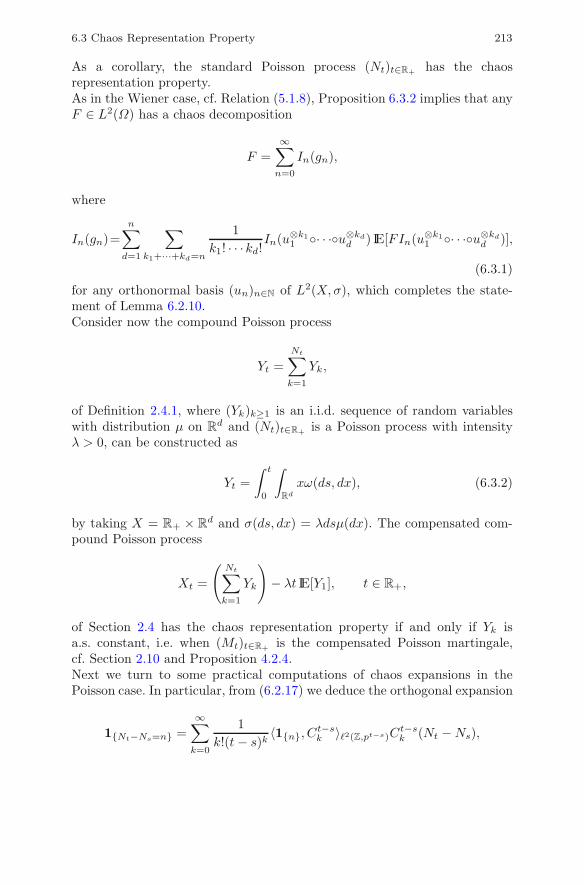
6.3 Chaos Representation Property 213
As a corollary, the standard Poisson process (Nt)t∈R+ has the chaosrepresentation property.As in the Wiener case, cf. Relation (5.1.8), Proposition 6.3.2 implies that anyF ∈ L2(Ω) has a chaos decomposition
F =∞∑
n=0
In(gn),
where
In(gn)=n∑
d=1
∑
k1+···+kd=n
1k1! · · ·kd!
In(u⊗k11 ◦· · ·◦u⊗kd
d ) IE[FIn(u⊗k11 ◦· · ·◦u⊗kd
d )],
(6.3.1)
for any orthonormal basis (un)n∈N of L2(X,σ), which completes the state-ment of Lemma 6.2.10.Consider now the compound Poisson process
Yt =Nt∑
k=1
Yk,
of Definition 2.4.1, where (Yk)k≥1 is an i.i.d. sequence of random variableswith distribution μ on R
d and (Nt)t∈R+ is a Poisson process with intensityλ > 0, can be constructed as
Yt =∫ t
0
∫
Rd
xω(ds, dx), (6.3.2)
by taking X = R+ × Rd and σ(ds, dx) = λdsμ(dx). The compensated com-
pound Poisson process
Xt =
(Nt∑
k=1
Yk
)− λt IE[Y1], t ∈ R+,
of Section 2.4 has the chaos representation property if and only if Yk isa.s. constant, i.e. when (Mt)t∈R+ is the compensated Poisson martingale,cf. Section 2.10 and Proposition 4.2.4.Next we turn to some practical computations of chaos expansions in thePoisson case. In particular, from (6.2.17) we deduce the orthogonal expansion
1{Nt−Ns=n} =∞∑
k=0
1k!(t− s)k
〈1{n}, Ct−sk 〉 2(Z,pt−s)C
t−sk (Nt −Ns),

214 6 Analysis on the Poisson Space
0 ≤ s ≤ t, n ∈ N, hence from (6.2.11):
1{Nt−Ns=n} =∞∑
k=0
1k!p(k)
n (t− s)Ik(1⊗k[s,t]), (6.3.3)
0 ≤ s ≤ t, n ∈ N.From (6.3.3) we obtain for s = 0 and n ≥ 1:
1[Tn,∞[(t) = 1{Nt≥n} (6.3.4)
=∞∑
k=0
∑
l≥n
1k!p(k)l (t)Ik(1⊗k
[0,t])
=∞∑
k=0
1k!∂kPn(t)Ik(1⊗k
[0,t]),
where
Pn(t) =∫ t
0
pn−1(s)ds, t ∈ R+, (6.3.5)
is the distribution function of Tn and pn(s) is defined in (2.3.1).More generally, we have the following result.Proposition 6.3.3. Let f ∈ C1
b (R+). We have
f(Tn) = −∞∑
k=0
1k!Ik
(∫ ∞
t1∨···∨tk
f ′(s)P (k)n (s)ds
), (6.3.6)
where t1 ∨ · · · ∨ tn = max(t1, . . . , tn), t1, . . . , tn ∈ R+.
Proof. We have
f(Tn) = −∫ ∞
0
f ′(s)1[Tn,∞)(s)ds
= −∫ ∞
0
f ′(s)∞∑
k=0
1k!P (k)
n (s)Ik(1⊗k[0,s])ds
= −∞∑
k=0
1k!
∫ ∞
0
f ′(s)P (k)n (s)Ik(1⊗k
[0,s])ds
= −∞∑
k=0
∫ ∞
0
f ′(s)P (k)n (s)
∫ s
0
∫ tk
0
· · ·∫ t2
0
dNt1 · · · dNtkds
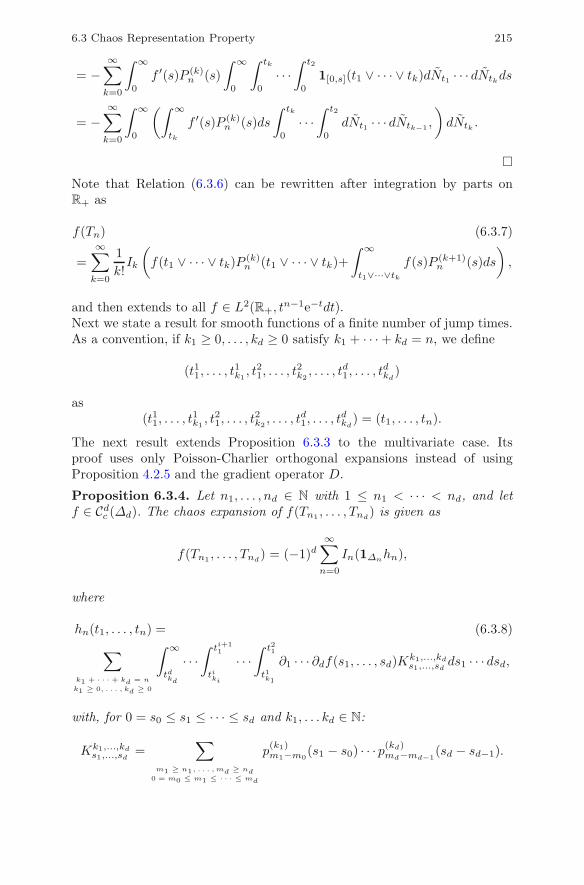
6.3 Chaos Representation Property 215
= −∞∑
k=0
∫ ∞
0
f ′(s)P (k)n (s)
∫ ∞
0
∫ tk
0
· · ·∫ t2
0
1[0,s](t1 ∨ · · · ∨ tk)dNt1 · · · dNtkds
= −∞∑
k=0
∫ ∞
0
(∫ ∞
tk
f ′(s)P (k)n (s)ds
∫ tk
0
· · ·∫ t2
0
dNt1 · · · dNtk−1 ,
)dNtk
.
�Note that Relation (6.3.6) can be rewritten after integration by parts onR+ as
f(Tn) (6.3.7)
=∞∑
k=0
1k!Ik
(f(t1 ∨ · · · ∨ tk)P (k)
n (t1 ∨ · · · ∨ tk)+∫ ∞
t1∨···∨tk
f(s)P (k+1)n (s)ds
),
and then extends to all f ∈ L2(R+, tn−1e−tdt).
Next we state a result for smooth functions of a finite number of jump times.As a convention, if k1 ≥ 0, . . . , kd ≥ 0 satisfy k1 + · · · + kd = n, we define
(t11, . . . , t1k1, t21, . . . , t
2k2, . . . , td1, . . . , t
dkd
)
as(t11, . . . , t
1k1, t21, . . . , t
2k2, . . . , td1, . . . , t
dkd
) = (t1, . . . , tn).
The next result extends Proposition 6.3.3 to the multivariate case. Itsproof uses only Poisson-Charlier orthogonal expansions instead of usingProposition 4.2.5 and the gradient operator D.
Proposition 6.3.4. Let n1, . . . , nd ∈ N with 1 ≤ n1 < · · · < nd, and letf ∈ Cd
c (Δd). The chaos expansion of f(Tn1 , . . . , Tnd) is given as
f(Tn1 , . . . , Tnd) = (−1)d
∞∑
n=0
In(1Δnhn),
where
hn(t1, . . . , tn) = (6.3.8)∑
k1 + · · · + kd = n
k1 ≥ 0, . . . , kd ≥ 0
∫ ∞
tdkd
· · ·∫ ti+1
1
tiki
· · ·∫ t21
t1k1
∂1 · · · ∂df(s1, . . . , sd)Kk1,...,kds1,...,sd
ds1 · · · dsd,
with, for 0 = s0 ≤ s1 ≤ · · · ≤ sd and k1, . . . kd ∈ N:
Kk1,...,kds1,...,sd
=∑
m1 ≥ n1, . . . , md ≥ nd0 = m0 ≤ m1 ≤ · · · ≤ md
p(k1)m1−m0
(s1 − s0) · · · p(kd)md−md−1
(sd − sd−1).

216 6 Analysis on the Poisson Space
Proof. Let 0 = s0 ≤ s1 ≤ · · · ≤ sd, and n1, . . . , nd ∈ N. We have from (6.3.3)and (6.2.16):
d∏
i=1
1{Nsi−Nsi−1=ni} =
∞∑
n=0
∑
k1 + · · · + kd = n
k1 ≥ 0, . . . , kd ≥ 0
1k1! · · · kd!
d∏
i=1
p(ki)mi−mi−1
(si − si−1)Ik1 (1⊗k1[s0,s1]) · · · Ikd
(1⊗kd
[sd−1,sd])
=∞∑
n=0
∑
k1 + · · · + kd = n
k1 ≥ 0, . . . , kd ≥ 0
1k1! · · · kd!
d∏
i=1
p(ki)mi−mi−1
(si − si−1)In(1⊗k1[s0,s1]
◦ · · · ◦ 1⊗kd
[sd−1,sd]),
where the last equality used the assumption s1 ≤ · · · ≤ sd. Now, with 0 =m0 ≤ m1 ≤ · · · ≤ md,
1[Tm1 ,Tm1+1[(s1) · · ·1[Tmd,Tmd+1[(sd) = 1{Ns1=m1} · · ·1{Nsd
=md}= 1{Ns1−Ns0=m1−m0} · · ·1{Nsd
−Nsd−1=md−md−1}
=∞∑
n=0
∑
k1 + · · · + kd = n
k1 ≥ 0, . . . , kd ≥ 0
1k1! · · ·kd!
d∏
i=1
p(ki)mi−mi−1
(si − si−1)In(1⊗k1[s0,s1] ◦ · · · ◦ 1⊗kd
[sd−1,sd]).
Given that s1 ≤ · · · ≤ sd, for any i < j the conditions si ∈ [Tmi , Tmi+1) andsj ∈ [Tmj , Tmj+1) imply mi ≤ mj , hence
d∏
i=1
1[Tni,∞)(si)=
∑
m1 ≥ n1, . . . , md ≥ nd0=m0 ≤ m1 ≤ · · · ≤ md
1[Tm1 ,Tm1+1[(s1) · · ·1[Tmd,Tmd+1[(sd)
=∑
m1 ≥ n1, . . . , md ≥ nd0 = m0 ≤ m1 ≤ · · · ≤ md
1{Ns1=m1} · · ·1{Nsd=md}
=∑
m1 ≥ n1, . . . , md ≥ nd0 = m0 ≤ m1 ≤ · · · ≤ md
1{Ns1−Ns0=m1−m0} · · ·1{Nsd−Nsd−1=md−md−1}
=∞∑
n=0
∑
k1 + · · · + kd = n
k1 ≥ 0, . . . , kd ≥ 0
1k1! · · ·kd!

6.3 Chaos Representation Property 217
∑
m1 ≥ n1, . . . , md ≥ nd0 = m0 ≤ m1 ≤ · · · ≤ md
p(k1)m1−m0
(s1 − s0) · · · p(kd)md−md−1
(sd − sd−1)
In(1⊗k1[s0,s1] ◦ · · · ◦ 1⊗kd
[sd−1,sd])
=∞∑
n=0
∑
k1 + · · · + kd = n
k1 ≥ 0, . . . , kd ≥ 0
1k1! · · ·kd!
Kk1,...,kds1,...,sd
In(1⊗k1[s0,s1]
◦ · · · ◦ 1⊗kd
[sd−1,sd]).
Given f ∈ Cdc (Δd), using the identity
f(Tn1 , . . . , Tnd)
= (−1)d∫ ∞
0
· · ·∫ ∞
0
1[Tn1 ,∞[(s1) · · ·1[Tnd,∞[(sd)
∂d
∂1 · · · ∂df(s1, . . . , sd)ds1 · · · dsd
= (−1)d∫
Δd
1[Tn1 ,∞[(s1) · · ·1[Tnd,∞[(sd)
∂d
∂1 · · · ∂df(s1, . . . , sd)ds1 · · · dsd,
we get
f(Tn1 , . . . , Tnd) = (−1)d
∞∑
n=0
∑
k1 + · · · + kd = n
k1 ≥ 0, . . . , kd ≥ 0
1k1! · · ·kd!
∫
Δd
∂d
∂1 · · · ∂df(s1, . . . , sd)Kk1,...,kd
s1,...,sdIn(1⊗k1
[s0,s1] ◦ · · · ◦ 1⊗kd
[sd−1,sd])ds1 · · · dsd.
From (6.2.16), we have for s1 ≤ · · · ≤ sd and k1 ≥ 0, . . . , kd ≥ 0:
In
(1⊗k1
[s0,s1] ◦ · · · ◦ 1⊗kd
[sd−1,sd]
)
= k1! · · · kd!∫ ∞
0
∫ tdkd
0
· · ·∫ t12
0
1⊗2[s0,s1]
(t11, t1k1
) · · ·1⊗2[sd−1,sd](t
d1, t
dkd
)
dNt11· · · dNtd
kd
,
hence by exchange of deterministic and stochastic integrals we obtain
f(Tn1 , . . . , Tnd) = (−1)d
∞∑
n=0
∑
k1 + · · · + kd = n
k1 ≥ 0, . . . , kd ≥ 0
In
(1Δn
∫ ∞
tdkd
∫ td1
td−1kd−1
· · ·∫ t31
t2k2
∫ t21
t1k1
∂df
∂s1 · · · ∂sd(s1, . . . , sd)Kk1,...,kd
s1,...,sdds1 · · · dsd
).
�

218 6 Analysis on the Poisson Space
Remarks
i) All expressions obtained above for f(T1, . . . , Td), f ∈ C∞b (Δd), extendto f ∈ L2(Δd, e−sdds1 · · ·dsd), i.e. to square-integrable f(T1, . . . , Td), byrepeated integrations by parts.ii) Chaotic decompositions on the Poisson space on the compact interval[0, 1] as in [79] or [80] can be obtained by considering the functional f(1∧T1, . . . , 1 ∧ Td) instead of f(T1, . . . , Td).
6.4 Finite Difference Gradient
In this section we study the probabilistic interpretation and the extension tothe Poisson space on X of the operators D and δ defined in Definitions 4.1.1and 4.1.2.Let the spaces S and U of Section 3.1 be taken equal to
S =
{n∑
k=0
Ik(fk) : fk ∈ L4(X)◦k, k = 0, . . . , n, n ∈ N
},
and
U =
{n∑
k=0
Ik(gk(∗, ·)) : gk ∈ L2(X)◦k ⊗ L2(X), k = 0, . . . , n, n ∈ N
}.
Definition 6.4.1. Let the linear, unbounded, closable operators
DX : L2(ΩX , πσ) → L2(ΩX ×X,P ⊗ σ)
andδX : L2(ΩX ×X,P ⊗ σ) → L2(ΩX ,P)
be defined on S and U respectively by
DXx In(fn) := nIn−1(fn(∗, x)), (6.4.1)
πσ(dω) ⊗ σ(dx)-a.e., n ∈ N, fn ∈ L2(X,σ)◦n, and
δX(In(fn+1(∗, ·))) := In+1(fn+1), (6.4.2)
πσ(dω)-a.s., n ∈ N, fn+1 ∈ L2(X,σ)◦n ⊗ L2(X,σ).
In particular we have
δX(f) = I1(f) =∫
X
f(x)(ω(dx) − σ(dx)), f ∈ L2(X,σ), (6.4.3)

6.4 Finite Difference Gradient 219
andδX(1A) = ω(A) − σ(A), A ∈ B(X), (6.4.4)
and the Skorohod integral has zero expectation:
IE[δX(u)] = 0, u ∈ Dom(δX). (6.4.5)
In case X = R+ we simply write D and δ instead of DR+ and δR+ .Note that using the mapping τ of Proposition 6.1.7 we have the relations
(Dτ(x)F ) ◦ τ∗ = DXx (F ◦ τ∗), πσ(dω) ⊗ σ(dx) − a.e.
andδ(uτ(·)) ◦ τ∗ = δX(u· ◦ τ∗), πσ(dω) − a.e.
From these relations and Proposition 4.1.4 we have the following proposition.
Proposition 6.4.2. For any u ∈ U we have
DXx δ
X(u) = u(x) + δX(DXx u). (6.4.6)
Let Dom (DX) denote the set of functionals F : ΩX → R with the expansion
F =∞∑
n=0
In(fn)
such that ∞∑
n=1
n!n‖fn‖2L2(Xn,σ⊗n) <∞,
and let Dom (δX) denote the set of processes u : ΩX × X → R with theexpansion
u(x) =∞∑
n=0
In(fn+1(∗, x)), x ∈ X,
such that ∞∑
n=0
(n+ 1)!‖fn+1‖2L2(Xn+1,σ⊗(n+1)) <∞.
The following duality relation can be obtained by transfer fromProposition 4.1.3 using Proposition 6.1.8. Here we also provide a directproof.Proposition 6.4.3. The operators DX and δX satisfy the duality relation
IE[〈DXF, u〉L2(X,σ)] = IE[FδX(u)], (6.4.7)
F ∈ Dom (DX), u ∈ Dom (δX).Proof. The proof is identical to those of Propositions 1.8.2 and 4.1.3, andfollows from the isometry formula (6.2.4). We consider F = In(fn) and ux =
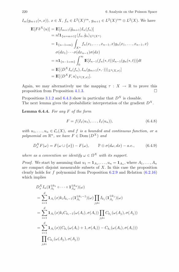
220 6 Analysis on the Poisson Space
Im(gm+1(∗, x)), x ∈ X , fn ∈ L2(X)◦n, gm+1 ∈ L2(X)◦m ⊗ L2(X). We have
IE[FδX(u)] = IE[Im+1(gm+1)In(fn)]= n!1{n=m+1}〈fn, gn〉L2(Xn)
= 1{n−1=m}
∫
Xn
fn(x1, . . . , xn−1, x)gn(x1, . . . , xn−1, x)
σ(dx1) · · ·σ(dxn−1)σ(dx)
= n1{n−1=m}
∫ ∞
0
IE[In−1(fn(∗, t))In−1(gn(∗, t))]dt
= IE[〈DX· In(fn), Im(gm+1(∗, ·))〉L2(X,σ)]
= IE[〈DXF, u〉L2(X,σ)].
Again, we may alternatively use the mapping τ : X → R to prove thisproposition from Proposition 4.1.3. �Propositions 3.1.2 and 6.4.3 show in particular that DX is closable.The next lemma gives the probabilistic interpretation of the gradient DX .
Lemma 6.4.4. For any F of the form
F = f(I1(u1), . . . , I1(un)), (6.4.8)
with u1, . . . , un ∈ Cc(X), and f is a bounded and continuous function, or apolynomial on R
n, we have F ∈ Dom (DX) and
DXx F (ω) = F (ω ∪ {x}) − F (ω), P ⊗ σ(dω, dx) − a.e., (6.4.9)
where as a convention we identify ω ∈ ΩX with its support.
Proof. We start by assuming that u1 = 1A1 , . . . , un = 1An , where A1, . . . , An
are compact disjoint measurable subsets of X . In this case the propositionclearly holds for f polynomial from Proposition 6.2.9 and Relation (6.2.16)which implies
DXx In(1⊗k1
A1◦ · · · ◦ 1⊗kd
Ad)(ω)
=d∑
i=1
1Ai(x)kiIki−1(1⊗ki−1Ai
)(ω)∏
j �=i
Ikj (1⊗kj
Aj)(ω)
=d∑
i=1
1Ai(x)kiCki−1(ω(Ai), σ(Ai))∏
j �=i
Ckj (ω(Aj), σ(Aj))
=d∑
i=1
1Ai(x)(Cki (ω(Ai) + 1, σ(Ai)) − Cki(ω(Ai), σ(Ai)))
∏
j �=i
Ckj (ω(Aj), σ(Aj))
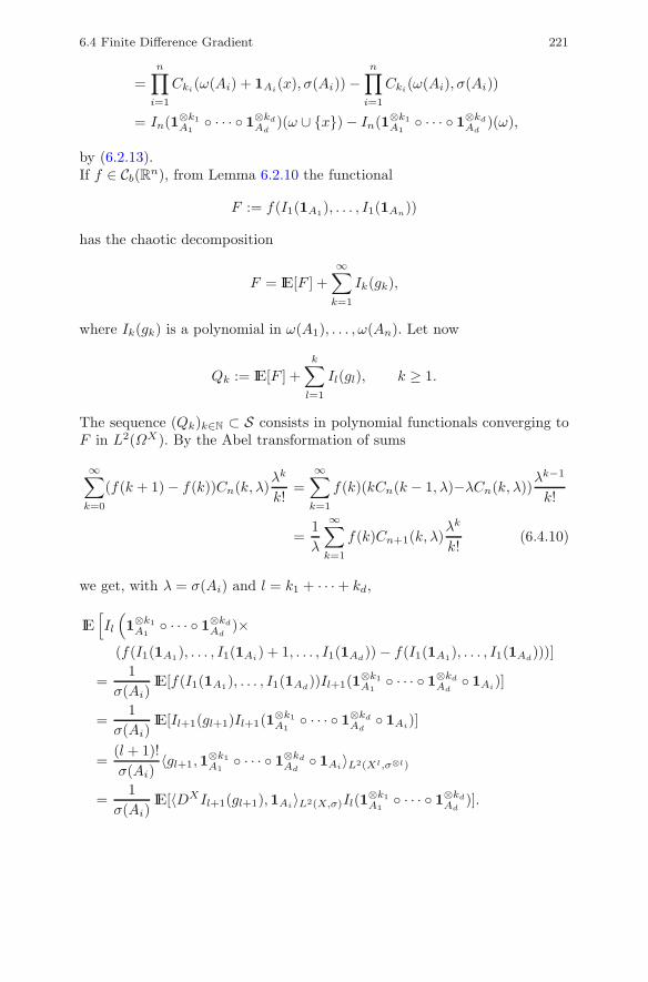
6.4 Finite Difference Gradient 221
=n∏
i=1
Cki(ω(Ai) + 1Ai(x), σ(Ai)) −n∏
i=1
Cki(ω(Ai), σ(Ai))
= In(1⊗k1A1
◦ · · · ◦ 1⊗kd
Ad)(ω ∪ {x}) − In(1⊗k1
A1◦ · · · ◦ 1⊗kd
Ad)(ω),
by (6.2.13).If f ∈ Cb(Rn), from Lemma 6.2.10 the functional
F := f(I1(1A1), . . . , I1(1An))
has the chaotic decomposition
F = IE[F ] +∞∑
k=1
Ik(gk),
where Ik(gk) is a polynomial in ω(A1), . . . , ω(An). Let now
Qk := IE[F ] +k∑
l=1
Il(gl), k ≥ 1.
The sequence (Qk)k∈N ⊂ S consists in polynomial functionals converging toF in L2(ΩX). By the Abel transformation of sums
∞∑
k=0
(f(k + 1) − f(k))Cn(k, λ)λk
k!=∞∑
k=1
f(k)(kCn(k − 1, λ)−λCn(k, λ))λk−1
k!
=1λ
∞∑
k=1
f(k)Cn+1(k, λ)λk
k!(6.4.10)
we get, with λ = σ(Ai) and l = k1 + · · · + kd,
IE[Il
(1⊗k1
A1◦ · · · ◦ 1⊗kd
Ad)×
(f(I1(1A1), . . . , I1(1Ai) + 1, . . . , I1(1Ad)) − f(I1(1A1), . . . , I1(1Ad
)))]
=1
σ(Ai)IE[f(I1(1A1), . . . , I1(1Ad
))Il+1(1⊗k1A1
◦ · · · ◦ 1⊗kd
Ad◦ 1Ai)]
=1
σ(Ai)IE[Il+1(gl+1)Il+1(1⊗k1
A1◦ · · · ◦ 1⊗kd
Ad◦ 1Ai)]
=(l + 1)!σ(Ai)
〈gl+1,1⊗k1A1
◦ · · · ◦ 1⊗kd
Ad◦ 1Ai〉L2(Xl,σ⊗l)
=1
σ(Ai)IE[〈DXIl+1(gl+1),1Ai〉L2(X,σ)Il(1
⊗k1A1
◦ · · · ◦ 1⊗kd
Ad)].
222 6 Analysis on the Poisson Space
Hence the projection of
f(I1(1A1), . . . , I1(1Ai) + 1, . . . , I1(1Ad)) − f(I1(1A1), . . . , I1(1Ad
))
on the chaos Hl of order l ∈ N is
1σ(Ai)
〈DXIl+1(gl+1),1Ai〉L2(X,σ),
and we have the chaotic decomposition
f(I1(1A1), . . . , I1(1Ai) + 1, . . . , I1(1Ad)) − f(I1(1A1), . . . , I1(1Ad
))
=1
σ(Ai)
∞∑
k=1
〈DXIk(gk),1Ai〉L2(X,σ),
where the series converges in L2(ΩX). Hence
n∑
i=1
1Ai(f(I1(1A1), . . . , I1(1Ai) + 1, . . . , I1(1Ad)) − f(I1(1A1), . . . , I1(1Ad
)))
=n∑
i=1
1σ(Ai)
1Ai
∞∑
k=1
〈DXIk(gk),1Ai〉L2(X,σ)
=∞∑
k=1
DXIk(gk)
= limn→∞D
XQn,
which shows that (DXQk)k∈N converges in L2(ΩX ×X) to
n∑
i=1
1Ai(f(I1(1A1), . . . , I1(1Ai) + 1, . . . , I1(1Ad)) − f(I1(1A1), . . . , I1(1Ad
))).
The proof is concluded by the closability of DX and approximation of func-tions in Cc(X) by linear combination of indicator functions. �
Definition 6.4.5. Given a mapping F : ΩX −→ R, let
ε+x F : ΩX −→ R and ε−x F : ΩX −→ R,
x ∈ X, be defined by
(ε−x F )(ω) = F (ω\x), and (ε+x F )(ω) = F (ω ∪ x), ω ∈ ΩX .

6.4 Finite Difference Gradient 223
Note that Relation (6.4.9) can be written as
DXx F = ε+x F − F, x ∈ X. (6.4.11)
On the other hand, the result of Lemma 6.4.4 is clearly verified on simplefunctionals. For instance when F = I1(u) is a single Poisson stochastic inte-gral, we have
DXx I1(u)(ω) = I1(u)(ω ∪ {x}) − I1(u)(ω)
=∫
X
u(y)(ω(dy) + εx(dy) − σ(dy)) −∫
X
u(y)(ω(dy) − σ(dy))
=∫
X
u(y)εx(dy)
= u(x).
Corollary 6.4.6. For all F is bounded and measurable A ∈ B(X), 0 <σ(A) <∞, we have
IE[∫
A
F (ω ∪ {x})σ(dx)]
= IE[Fω(A)]. (6.4.12)
Proof. From Proposition 6.4.3, Lemma 6.4.4, and Relation (6.4.4) we have
IE[∫
A
F (ω ∪ {x})σ(dx)]
= IE[∫
X
1A(x)DxFσ(dx)]
+ σ(A) IE[F ]
= IE[FδX(1A)] + σ(A) IE[F ]= IE[Fω(A)].
�Hence as in [150] we get that the law of the mapping (x, ω) �→ ω ∪{x} under1A(x)σ(dx)πσ(dω) is absolutely continuous with respect to πσ . In particular,(ω, x) �→ F (ω ∪ {x}) is well-defined, πσ ⊗ σ, and this justifies the extensionof Lemma 6.4.4 in the next proposition.
Proposition 6.4.7. For any F ∈ Dom (DX) we have
DXx F (ω) = F (ω ∪ {x}) − F (ω),
πσ(dω) × σ(dx)-a.e.
Proof. There exists a sequence (Fn)n∈N of functionals of the form (6.4.8),such that (DXFn)n∈N converges everywhere to DXF on a set AF such that(πσ⊗σ)(Ac
F ) = 0. For each n ∈ N, there exists a measurable set Bn ⊂ ΩX×Xsuch that (πσ ⊗ σ)(Bc
n) = 0 and

224 6 Analysis on the Poisson Space
DXx Fn(ω) = Fn(ω ∪ {x}) − Fn(ω), (ω, x) ∈ Bn.
Taking the limit as n goes to infinity on (ω, x) ∈ AF ∩⋂∞n=0Bn, we get
DXx F (ω) = F (ω ∪ {x}) − F (ω), πσ(dω) × σ(dx) − a.e.
�Proposition 6.4.7 also allows us to recover the annihilation property (6.4.1)of DX , i.e.:
DXx In(fn) = nIn−1(fn(∗, x)), σ(dx) − a.e. (6.4.13)
Indeed, using the relation
1Δn(x1, . . . , xn)εx(dxi)εx(dxj) = 0, i, j = 1, . . . , n,
we have for fn ∈ L2(X,σ)◦n:
DXx In(fn) = DX
x
∫
Δn
fn(x1, . . . xn)(ω(dx1) − σ(dx1)) · · · (ω(dxn) − σ(dxn))
=∫
Δn
fn(x1, . . . , xn)n∏
i=1
(ω(dxi) − σ(dxi) + (1 − ω({x}))εx(dxi))
−∫
Δn
fn(x1, . . . , xn)(ω(dx1) − σ(dx1)) · · · (ω(dxn) − σ(dxn))
= (1 − ω({x}))n∑
i=1
∫
Δn−1
fn(x1, . . . , x, . . . , xn)∏
1≤k �=i≤n
(ω(dxk) − σ(dxk))
= (1 − ω({x}))n∑
i=1
In−1(fn( · · ·︸︷︷︸i−1
, x, · · ·︸︷︷︸n−i
)), x ∈ X.
Hence we have for fn ∈ Cc(Xn):
DXx In(fn) = 1{x/∈ω}
n∑
i=1
In−1(fn( · · ·︸︷︷︸i−1
, x, · · ·︸︷︷︸n−i
)), x ∈ X,
and since fn is symmetric,
DXx In(fn) = 1{x/∈ω}nIn−1(fn(∗, x)), x ∈ X,
from which we recover (6.4.13) since σ is diffuse.Proposition 6.4.7 implies that DX satisfies the following finite differenceproduct rule.

6.4 Finite Difference Gradient 225
Proposition 6.4.8. We have for F,G ∈ S:
DXx (FG) = FDX
x G+GDXx F +DX
x FDXx G, (6.4.14)
P(dω)dσ(x)-a.e.
Proof. This formula can be proved either from Propositions 4.5.2 and 6.1.8with φt = 1, t ∈ R+, when X = R+, or directly from (6.4.9):
DXx (FG)(ω) = F (ω ∪ {x})G(ω ∪ {x}) − F (ω)G(ω)
= F (ω)(G(ω ∪ {x}) −G(ω)) +G(ω)(F (ω ∪ {x}) − F (ω))+(F (ω ∪ {x}) − F (ω))(G(ω ∪ {x}) −G(ω))
= F (ω)DXx G(ω) +G(ω)DX
x F (ω) +DXx F (ω)DX
x G(ω),
dP × σ(dx)-a.e. �As a consequence of Proposition 6.4.7 above, whenX = R+ the Clark formulaProposition 4.2.3 takes the following form when stated on the Poisson space.
Proposition 6.4.9. Assume that X = R+. For any F ∈ Dom (D) we have
F = IE[F ] +∫ ∞
0
IE[F (ω ∪ {t})− F (ω) | Ft]d(Nt − t).
In case X = R+ the finite difference operator D : L2(Ω) −→ L2(Ω × R+)can be written as
DtF = 1{Nt<n}(f(T1, . . . , TNt , t, TNt+1, . . . , Tn−1)−f(T1, . . . , Tn)), (6.4.15)
t ∈ R+, for F = f(T1, . . . , Tn), hence IE[DtF |Ft] can be computed via thefollowing lemma.
Lemma 6.4.10. Let X = R+ and σ(dx) = dx. For any F of the formF = f(T1, . . . , Tn) we have
IE[DtF |Ft]
= 1{Nt<n}
∫ ∞
t
e−(sn−t)
∫ sn
t
· · ·∫ sNt+3
t(f(T1, . . . , TNt, t, sNt+2, . . . , sn) −
∫ sNt+2
t
f(T1, . . . , TNt, sNt+1, . . . , sn)dsNt+1
)
dsNt+2 · · · dsn.
Proof. By application of Proposition 2.3.6 we have
IE[DtF |Ft]= 1{Nt<n} IE[f(T1, . . . , TNt , t, TNt+1, . . . , Tn−1) − f(T1, . . . , Tn)|Ft]

226 6 Analysis on the Poisson Space
= 1{Nt<n}
∫ ∞
t
e−(sn−t)
∫ sn
t
· · ·∫ sNt+3
t
f(T1, . . . , TNt , t, sNt+2, . . . , sn)
dsNt+2 · · · dsn
−1{Nt<n}
∫ ∞
t
e−(sn−t)
∫ sn
t
· · ·∫ sNt+2
t
f(T1, . . . , TNt, sNt+1, . . . , sn)
dsNt+1 · · · dsn
= 1{Nt<n}
∫ ∞
t
e−(sn−t)
∫ sn
t
· · ·∫ sNt+3
t(f(T1, . . . , TNt, t, sNt+2, . . . , sn) −
∫ sNt+2
t
f(T1, . . . , TNt, sNt+1, . . . , sn)dsNt+1
)
dsNt+2 · · · dsn.
�
6.5 Divergence Operator
The adjoint δX of DX satisfies the following divergence formula.
Proposition 6.5.1. Let u : X × ΩX −→ R and F : ΩX −→ R such thatu(·, ω), DX
· F (ω), and u(·, ω)DX· F (ω) ∈ L1(X,σ), ω ∈ ΩX . We have
FδX(u) = δX(uF ) + 〈u,DXF 〉L2(X,σ) + δX(uDXF ). (6.5.1)
The relation also holds if the series and integrals converge, or if F ∈Dom (DX) and u ∈ Dom (δX) is such that uDXF ∈ Dom (δX).
Proof. Relation (6.5.1) follows by duality from Proposition 6.4.8, or fromProposition 4.5.6 and Proposition 6.1.8. �In the next proposition, Relation (6.5.2) can be seen as a generalization of(6.2.14) in Proposition 6.2.8:
Cn+1(k, t) = kCn(k − 1, t) − tCn(k, t),
which is recovered by taking u = 1A and t = σ(A). The following state-ment provides a connection between the Skorohod integral and the Poissonstochastic integral.
Proposition 6.5.2. For all u ∈ Dom (δX) we have
δX(u) =∫
X
ux(ω \ {x})(ω(dx) − σ(dx)). (6.5.2)
Proof. The statement clearly holds by (6.4.3) when g ∈ L2(X,σ) is deter-ministic. Next we show using (6.5.1) that the identity also holds for a process

6.5 Divergence Operator 227
of the form u = gIn(fn), g ∈ L2(X,σ), by induction on the order of themultiple stochastic integral F = In(fn). From (6.5.1) we have
δX(gF ) = −δX(gDXF ) + FδX(g) − 〈DXF, g〉L2(X,σ)
= −∫
X
g(x)DXx F (ω\{x})ω(dx) +
∫
X
g(x)DXx F (ω\{x})σ(dx)
+FδX(g) − 〈DXF, g〉L2(X,σ)
= −∫
X
g(x)F (ω)ω(dx) +∫
X
g(x)F (ω\{x})ω(dx) + 〈DXF (ω), g〉L2(X,σ)
+FδX(g) − 〈DXF, g〉L2(X,σ)
= −F (ω)∫
X
g(x)σ(dx) +∫
X
g(x)F (ω\{x})ω(dx)
=∫
X
g(x)F (ω\{x})ω(dx) −∫
X
g(x)F (ω\{x})σ(dx).
We used the fact that since σ is diffuse on X , for u : X ×ΩX −→ R we have
ux(ω\{x}) = ux(ω), σ(dx) − a.e., ω ∈ ΩX ,
hence∫
X
ux(ω\{x})σ(dx) =∫
X
ux(ω)σ(dx), ω ∈ ΩX , (6.5.3)
and
δX(u) =∫
X
ux(ω\{x})ω(dx) −∫
X
ux(ω)σ(dx), u ∈ Dom(δX).
�Note that (6.5.1) can also be recovered from (6.5.2) using a simple trajectorialargument. For x ∈ ω we have
ε−x DXx F (ω) = ε−x ε
+x F (ω) − ε−x F (ω)
= F (ω) − ε−x F (ω)= F (ω) − F (ω\{x}),
hence
δX(uDXF )(ω)
=∫
X
ux(ω\{x})DXx F (ω\{x})ω(dx) −
∫
X
ux(ω\{x})DXx F (ω\{x})σ(dx)
=∫
X
ux(ω\{x})F (ω)ω(dx) −∫
X
ux(ω\{x})F (ω\{x})ω(dx)
−〈DXF (ω), u(ω)〉L2(X,σ)
= F (ω)δX(u)(ω) − δX(uF )(ω) − 〈DXF (ω), u(ω)〉L2(X,σ),

228 6 Analysis on the Poisson Space
since from Relation (6.5.3),
F (ω)∫
X
ux(ω\{x})σ(dx) = F (ω)∫
X
ux(ω)σ(dx)
=∫
X
F (ω\{x})ux(ω\{x})σ(dx).
Relation (6.5.2) can also be proved using Relation (6.2.3).In case X = R+, Proposition 6.5.2 yields Proposition 2.5.10 since ut−
does not depend on the presence of a jump at time t. On the other hand,Proposition 4.3.4 can be written as follows.
Proposition 6.5.3. When X = R+, for any square-integrable adapted pro-cess (ut)t∈R+ ∈ L2
ad(Ω × R+) we have
δ(u) =∫ ∞
0
utd(Nt − t).
The following is the Skorohod isometry on the Poisson space, which followshere from Proposition 6.5.1, or from Propositions 4.3.1 and 6.1.8.
Proposition 6.5.4. For u : ΩX ×X → R measurable and sufficiently inte-grable we have
IEπσ
[|δX(u)|2] = IE[‖u‖2
L2(X,σ)
]+ IE
[∫
X
∫
X
DXx u(y)DX
y u(x)σ(dx)σ(dy)].
(6.5.4)
Proof. Applying Proposition 6.4.2, Proposition 6.5.1 and Relation (6.4.5) wehave
IEπσ
[|δX(u)|2]
= IEπσ
[δX(uδX(u)) + 〈u,DXδX(u)〉L2(X,σ) + δX(uDXδX(u))
]
= IEπσ
[〈u,DXδX(u)〉L2(X,σ)
]
= IEπσ
[‖u‖2
L2(X,σ) +∫
X
u(x)δX(DXx u)σ(dx)
]
= IEπσ
[‖u‖2
L2(X,σ) +∫
X
∫
X
DXy u(x)DX
x u(y)σ(dx)σ(dy)].
�The Skorohod isometry (6.5.4) shows that δX is continuous on the subspaceIL1,2 of L2(X ×ΩX) defined by the norm
‖u‖21,2 = ‖u‖2
L2(ΩX×X)) + ‖DXu‖2L2(ΩX×X2).

6.5 Divergence Operator 229
Recall that the moment IEλ[Zn] of order n of a Poisson random variable Zwith intensity λ can be written as
IEλ[Zn] = Tn(λ)
where Tn(λ) is the Touchard polynomial of order n, defined by T0(λ) = 1and the recurrence relation
Tn(λ) = λn∑
k=0
(n
k
)Tk(λ), n ≥ 1. (6.5.5)
Replacing the Touchard polynomial Tn(λ) by its centered version Tn(λ) de-fined by T0(λ) = 1, i.e.
Tn+1(λ) =n−1∑
k=0
(n
k
)λn−k+1Tk(λ), n ≥ 0, (6.5.6)
gives the moments of the centered Poisson random variable with intensityλ > 0 is
Tn(λ) = IE[(Z − λ)n], n ≥ 0.
The next proposition extends the Skorohod isometry of Proposition 6.5.4 tohigher order moments, and recovers Proposition 6.5.4 in case n = 1.
Proposition 6.5.5. We have, for u : ΩX ×X → R a sufficiently integrableprocess,
IE[(δX(u))n+1] =n−1∑
k=0
(n
k
)IE[∫
X
(ut)n−k+1(δX(u))kσ(dt)]
+n∑
k=1
(n
k
)IE[∫
X
(ut)n−k+1((δX((I +DXt )u))k − (δX(u))k)σ(dt)
],
for all n ≥ 1.
Proof. Using the relation
DXt (δX(u))n = ε+t (δX(u))n − (δX(u))n
= (ε+t δX(u))n − (δX(u))n
= (δX(u) +DXt δ
X(u))n − (δX(u))n
= (δX(u) + ut + δX(DXt u))n − (δX(u))n, t ∈ X,
that follows from Proposition 6.4.2 and Relation (6.4.11), we get, applyingthe duality relation of Proposition 6.4.3,

230 6 Analysis on the Poisson Space
IE[(δX(u))n+1] = IE[∫
X
u(t)DXt (δX(u))nσ(dt)
]
= IE[∫
X
ut((δX(u) + ut + δX(DXt u))n − (δX(u))n)σ(dt)
]
=n∑
k=0
(n
k
)IE[∫
X
(ut)n−k+1(δX((I +DXt )u))kσ(dt)
]
− IE[(δX(u))n
∫
X
utσ(dt)]
=n−1∑
k=0
(n
k
)IE[∫
X
(ut)n−k+1(δX(u))kσ(dt)]
+n∑
k=1
(n
k
)IE[∫
X
(ut)n−k+1((δX((I +DXt )u))k − (δX(u))k)σ(dt)
].
�Clearly, the moments of the compensated Poisson stochastic integral
∫
X
f(t)(ω(dt) − σ(dt))
of f ∈ L2(X,σ) satisfy the recurrence identity
IE
[(∫
X
f(t)(ω(dt) − σ(dt)))n+1
]
=n−1∑
k=0
(n
k
)∫
X
(f(t))n−k+1σ(dt) IE
[(∫
X
f(t)(ω(dt) − σ(dt)))k],
which is analog to Relation (6.5.6) for the centered Touchard polynomialsand recovers in particular the isometry formula (6.1.7) for n = 1. Similarlywe can show that
IE
[(∫
X
f(s)ω(ds))n+1
](6.5.7)
=n∑
k=0
(n
k
)IE
[(∫
X
f(s)ω(ds))k ∫
X
(f(t))n+1−kσ(dt)
],
which is analog to (6.5.5).

6.6 Characterization of Poisson Measures 231
6.6 Characterization of Poisson Measures
The duality relation (6.4.7) satisfied by the operators DX and δX can alsobe used to characterize Poisson measures.
Proposition 6.6.1. Let π be a probability measure on ΩX such that h ∈C∞c (X), I1(h) has finite moments of all orders under π. Assume that
IEπ
[δX(u)
]= 0, (6.6.1)
for all u ∈ U , or equivalently
IEπ
[〈DXF, h〉L2(X,σ)
]= IEπ
[FδX(h)
], (6.6.2)
F ∈ S, h ∈ C∞c (X). Then π is the Poisson measure πσ with intensity σ.
Proof. First, we note that from Remark 6.2.6, if I1(h) has finite moments ofall orders under π, for all h ∈ C∞c (X), then δX(u) is integrable under π forall u ∈ U . Next we show that (6.6.1) and (6.6.2) are equivalent. First we notethat Relation (6.6.1) implies (6.6.2) from (6.5.1). The proof of the conversestatement is done for u of the form u = hF , F = In(f⊗n), f, h ∈ C∞c (X),by induction on the degree n ∈ N of In(f⊗n). The implication clearly holdswhen n = 0. Next, assuming that
IEπ
[δX(hIn(f⊗n))
]= 0, f, h ∈ C∞c (X),
for some n ≥ 0, the Kabanov multiplication formula (6.2.5) shows that
δX(hIn+1(f⊗(n+1))) = δX(h)In+1(f⊗(n+1)) − 〈h,DXIn+1(f⊗(n+1))〉L2(X,σ)
−(n+ 1)δX((hf)In(f⊗n)),
hence from Relation (6.6.1) applied at the rank n we have
IEπ
[δX(hIn+1(f⊗n+1))
]= IEπ
[δX(h)In+1(f⊗(n+1))
]
− IEπ
[〈h,DXIn+1(f⊗(n+1))〉L2(X,σ)
]
−(n+ 1) IEπ
[δX((hf)In(f⊗n))
]
= IEπ
[δX(h)In+1(f⊗(n+1))
]
− IEπ
[〈h,DXIn+1(f⊗(n+1))〉L2(X,σ)
]
= 0,
by (6.6.2).

232 6 Analysis on the Poisson Space
Next we show that π = πσ. We have for h ∈ C∞c (X) and n ≥ 1, using (6.6.2):
IEπ
[(∫
X
h(x)ω(dx))n]
= IEπ
[δX(h)
(∫
X
h(x)ω(dx))n−1
]
+(∫
X
h(x)σ(dx))
IEπ
[(∫
X
h(x)ω(dx))n−1
]
= IEπ
⎡
⎣⟨h,DX
(∫
X
h(x)ω(dx))n−1
⟩
L2(X,σ)
⎤
⎦
+(∫
X
h(x)σ(dx))
IEπ
[(∫
X
h(x)ω(dx))n−1
]
= IEπ
[∫
X
h(x)(h(x) +
∫
X
h(y)(ω\{x})(dy))n−1
σ(dx)
]
= IEπ
[∫
X
h(x)(h(x) +
∫
X
h(y)ω(dy))n−1
σ(dx)
]
=n−1∑
k=0
(n− 1k
)(∫
X
hn−k(x)σ(dx))
IEπ
[(∫
X
h(x)ω(dx))k].
This induction relation coincides with (6.5.7) and characterizes the moments
of ω �→∫
X
h(x)ω(dx) under πσ, hence the moments of ω �→∫
X
h(x)ω(dx)
under π are that of a Poisson random variable with intensity∫
X
h(x)σ(dx).
By dominated convergence this implies
IEπ
[exp
(iz
∫
X
h(x)ω(dx))]
= exp∫
X
(eizh − 1)dσ,
z ∈ R, h ∈ C∞c (X), hence π = πσ. �This proposition can be modified as follows.
Proposition 6.6.2. Let π be a probability measure on ΩX such that δX(u)is integrable, u ∈ U . Assume that
IEπ
[δX(u)
]= 0, u ∈ U , (6.6.3)
or equivalently
IEπ
[〈DXF, u〉L2(X,σ)
]= IEπ
[FδX(u)
], F ∈ S, u ∈ U . (6.6.4)
Then π is the Poisson measure πσ with intensity σ.
6.6 Characterization of Poisson Measures 233
Proof. Clearly, (6.6.3) implies (6.6.4) as in the proof of Proposition 6.6.1. Theimplication (6.6.4) ⇒ (6.6.3) follows in this case by taking F = 1. Denotingthe characteristic function of ω �→ ∫
X h(x)ω(dx) by
ψ(z) = IEπ
[exp
(iz
∫
X
h(y)ω(dy))]
,
z ∈ R, we have:
dψ
dz(z) = i IEπ
[∫
X
h(y)ω(dy) exp(iz
∫
X
h(y)ω(dy))]
= i IEπ
[δX(h) exp
(iz
∫
X
h(y)ω(dy))]
+i IEπ
[∫
X
h(y)σ(dy) exp(iz
∫
X
h(y)ω(dy))]
= i IEπ
[⟨h,DX exp
(iz
∫
X
h(y)ω(dy))⟩
L2(X,σ)
]+ iψ(z)
∫
X
h(y)σ(dy)
= i〈h, eizh − 1〉L2(X,σ) IEπ
[exp
(iz
∫
X
h(y)ω(dy))]
+ iψ(z)∫
X
h(y)σ(dy)
= iψ(z)〈h, eizh〉L2(X,σ), z ∈ R.
We used the relation
DXx exp
(iz
∫
X
h(y)ω(dy))
= (eizh(x)−1) exp(iz
∫
X
h(y)ω(dy)), x ∈ X,
that follows from Proposition 6.4.7. With the initial condition ψ(0) = 1 weobtain
ψ(z) = exp∫
X
(eizh(y) − 1)σ(dy), z ∈ R.
�
Corollary 6.6.3. Let π be a probability measure on ΩX such that In(f⊗n)is integrable under π, f ∈ C∞c (X). The relation
IEπ
[In(f⊗n)
]= 0, (6.6.5)
holds for all f ∈ C∞c (X) and n ≥ 1, if and only if π is the Poisson measureπσ with intensity σ.
Proof. If (6.6.5) holds then by polarization and the Definition 6.4.2 we get
IEπ
[δX(g ⊗ In(f1 ⊗ · · · ⊗ fn))
]= 0,

234 6 Analysis on the Poisson Space
g, f1, . . . , fn ∈ C∞c (X), n ≥ 0, and from Remark 6.2.6 we have
IEπ[δX(u)] = 0, u ∈ U ,
hence π = πσ from Proposition 6.6.1. �
6.7 Clark Formula and Levy Processes
In this section we extend the construction of the previous section to the caseof Levy processes, and state a Clark formula in this setting. Let X = R+×R
d
and consider a random measure of the form
X(dt, dx) = δ0(dx)dBt + ω(dt, dx) − σ(dx)dt,
where ω(dt, dx) − σ(dx)dt is a compensated Poisson random measure onR
d \{0}×R+ of intensity σ(dx)dt, and (Bt)t∈R+ is a standard Brownian mo-tion independent of N(dt, dx). The underlying probability space is denotedby (Ω,F ,P), where F is generated by X . We define the filtration (Ft)t∈R+
generated by X as
Ft = σ(X(ds, dx) : x ∈ Rd, s ≤ t).
The integral of a square-integrable (Ft)t∈R+ -adapted process u ∈ L2(Ω) ⊗L2(Rd × R+) with respect to X(dt, dx) is written as
∫
Rd×R+
u(t, x)X(dt, dx),
with the isometry
IE
⎡
⎣(∫
Rd×R+
u(t, x)X(dt, dx)
)2⎤
⎦ = IE
[∫
Rd×R+
|u(t, x)|2σ(dx)dt
], (6.7.1)
withσ(dx) = δ0(dx) + σ(dx).
The multiple stochastic integral In(hn) of hn ∈ L2(Rd×R+)◦n can be definedby induction with
I1(h) =∫
Rd×R+
h(t, x)X(dt, dx)
=∫ ∞
0
h(0, t)dBt +∫
Rd\{0}×R+
h(t, x)(ω(dt, dx) − σ(dx)dt),

6.7 Clark Formula and Levy Processes 235
h ∈ L2(Rd × R+), and
In(hn) = n
∫
Rd×R+
In−1(πnt,xhn)X(dt, dx),
whereπn
t,x : L2(Rd × R+)◦n −→ L2(Rd × R+)◦(n−1) (6.7.2)
is defined by
[πn
t,xhn
](x1, t1, . . . , xn−1, tn−1)
= hn(x1, t1, . . . , xn−1, tn−1, t, x)1[0,t](t1) · · ·1[0,t](tn−1),
for x1, . . . , xn−1, x ∈ Rd and t1, . . . , tn−1, t ∈ R+.
As in (6.1.9) the characteristic function of I1(h) is given by
IE[eizI1(h)
]
= exp
(−z
2
2
∫ ∞
0
h(0, t)2dt+∫
Rd\{0}×R+
(eizh(t,x) − 1 − izh(t, x))σ(dx)dt
).
The isometry property
IE[|In(hn)|2] = n!‖hn‖2
L2(Rd×R+)⊗n ,
follows from Relation (6.7.1).From Proposition 5.1.5 and Proposition 6.3.2, every F ∈ L2(Ω) admits adecomposition
F = IE[F ] +∑
n≥1
1n!In(fn) (6.7.3)
into a series of multiple stochastic integrals, with fn ∈ L2(Rd×R+)◦n, n ≥ 1.The next proposition is a version of the Clark predictable representationformula for Levy processes.
Proposition 6.7.1. For F ∈ L2(Ω), we have
F = IE[F ] +∫
Rd×R+
IE[DXt,xF | Ft]X(dt, dx). (6.7.4)
Proof. Let
Δn ={((x1, t1), . . . , (xn, tn)) ∈ (Rd × R+)n : t1 < · · · < tn
}.

236 6 Analysis on the Poisson Space
From (6.7.3) we have for F ∈ S:
F = IE[F ] +∑
n≥1
In(fn1Δn)
= IE[F ] +∑
n≥1
∫
Rd×R+
In−1(fn(·, t, x)1Δn(·, t, x))X(dt, dx)
= IE[F ] +∫
Rd×R+
∞∑
n=0
IE[In(fn+1(·, t, x)1Δn) | Ft]X(dt, dx)
= IE[F ] +∫
Rd×R+
IE[DXt,xF | Ft]X(dt, dx)
The extension of this statement to F ∈ L2(Ω) is a consequence of the factthat the adapted projection of DXF extends to a continuous operator fromL2(Ω) into the space of adapted processes in L2(Ω) ⊗ L2(Rd × R+). For
F =∞∑
n=0
In(fn) ∈ S
and
u =∞∑
n=0
In(un+1) ∈ U , un+1 ∈ L2(Rd × R+)◦n ⊗ L2(Rd × R+), n ∈ N,
we can extend the continuity argument of Proposition 3.2.6 as follows:∣∣∣∣∣IE
[∫
Rd×R+
u(t, x) IE[DXt,xF | Ft]σ(dx)dt
]∣∣∣∣∣
≤∞∑
n=0
(n+ 1)!∣∣∣∫
Rd×R+
〈fn+1(·, t, x)1[0,t](·), un+1(·, t, x)〉L2(Rd×R+)⊗nσ(dx)dt∣∣∣
≤∞∑
n=0
(n+ 1)!‖fn+1‖L2(Rd×R+)‖un+1‖L2(Rd×R+)⊗(n+1)
≤( ∞∑
n=0
n!‖fn‖2L2(Rd×R+)⊗n
∞∑
n=0
n!‖un+1‖2L2(Rd×R+)⊗(n+1)
)1/2
≤ ‖F‖L2(Ω)‖u‖L2(Ω)⊗L2(Rd×R+).
�Note that Relation (6.7.4) can be written as
F = IE[F ] +∫
Rd×R+
IE[DXt,0F | Ft]dBt
+∫
Rd×R+
IE[DXt,xF | Ft](ω(dt, dx) − σ(dx)dt).

6.8 Covariance Identities 237
6.8 Covariance Identities
The Ornstein-Uhlenbeck semi-group satisfies
PtIn(fn) = e−ntIn(fn), fn ∈ L2(X)◦n, n ∈ N.
We refer to [140] for the construction of the ΩX -valued diffusion process as-sociated to (Pt)t∈R+ . Here we shall only need the existence of the probabilitydensity kernel associated to (Pt)t∈R+ .
Lemma 6.8.1. In case σ is finite on X we have
PtF (ω) =∫
ΩX×ΩX
F (ω ∪ ω)qt(ω, dω, dω), ω ∈ ΩX , (6.8.1)
where qt(ω, dω, dω) is the probability kernel on ΩX ×ΩX defined by
qt(ω, dω, dω) =∑
ω′⊂ω
|ω|!|ω′|!|ω\ω′|! (e
−t)|ω′|(1 − e−t)|ω−ω′|εω′(dω)π(1−e−t)σ(dω).
Here, π(1−e−t)σ is the thinned Poisson measure with intensity (1−e−t)σ(dx),εω denote the Dirac measure at ω ∈ ΩX and |ω| = ω(X) ∈ N\{0} ∪ {+∞}represents the (πσ-a.s. finite) cardinal of ω ∈ ΩX .
Proof. We consider random functionals of the form
F = e−∫
Xu(x)σ(dx)
∏
x∈ω
(1 + u(x)) =∞∑
k=0
1n!In(u⊗n),
cf. Proposition 6.3.1, for which we have
PtF =∞∑
n=0
1n!
e−ntIn(u⊗n) = exp(−e−t
∫
X
u(x)σ(dx)) ∏
x∈ω
(1 + e−tu(x)),
and∫
ΩX×ΩX
F (ω ∪ ω)P(ω, dω, dω)
= exp(−∫
X
u(x)σ(dx))∫
ΩX
∫
ΩX
∑
ω′⊂ω
∏
x∈ω∪ω
(1 + u(x))|ω|!
|ω′|!|ω\ω′|! e−t|ω′|(1 − e−t)|ω−ω′|εω(dω)π(1−e−t)σ(dω)
= exp(−e−t
∫
X
u(x)σ(dx))
238 6 Analysis on the Poisson Space
∫
ΩX
∑
ω′⊂ω
∏
x∈ω
(1 + u(x))|ω|!
|ω′|!|ω\ω′|! e−t|ω′|(1 − e−t)|ω−ω′|εω(dω)
= exp(−e−t
∫
X
u(x)σ(dx))
∑
ω′⊂ω
∏
x∈ω′(1 + u(x))
|ω|!|ω′|!|ω\ω′|! e
−t|ω′|(1 − e−t)|ω−ω′|
= exp(−e−t
∫
X
u(x)σ(dx))
∑
ω′⊂ω
|ω|!|ω′|!|ω\ω′|!
∏
x∈ω′e−t(1 + u(x))
∏
x∈ω\ω′(1 − e−t)
= exp(−e−t
∫
X
u(x)σ(dx)) ∏
x∈ω
(1 + e−tu(x))
= PtF (ω).�
The semi-group Pt can be rewritten as
PtF (ω) =∑
ω′⊂ω
|ω|!|ω′|!|ω\ω′|! e
−t|ω′|(1− e−t)|ω−ω′|∫
ΩX
F (ω′ ∪ ω)π(1−e−t)σ(dω).
Again, Lemma 6.8.1 and Jensen’s inequality (9.3.1) imply
‖Ptu‖L2(R+) ≤ ‖u‖L2(R+), u ∈ L2(ΩX × R+),
a.s., hence‖Ptu‖L∞(ΩX ,L2(R+)) ≤ ‖u‖L∞(ΩX ,L2(R+)),
t ∈ R+, u ∈ L2(ΩX × R+). A covariance identity can be written using theOrnstein-Uhlenbeck semi-group, in the same way as in Proposition 4.4.1.
Proposition 6.8.2. We have the covariance identity
Cov (F,G) = IE[∫ ∞
0
∫
X
e−sDXx FPsD
Xx Gσ(dx)ds
], (6.8.2)
F,G ∈ Dom (DX).
Proof. By the chaos representation property Proposition 6.3.2, orthogonalityof multiple integrals of different orders, and continuity of Ps, s ∈ R+, onL2(ΩX ,P), it suffices to prove the identity for F = In(fn) and G = In(gn).We have

6.8 Covariance Identities 239
IEπσ [In(fn)In(gn)] = n!〈fn, gn〉L2(X,σ)◦n
= n!∫
Xn
fn(x1, . . . , xn)gn(x1, . . . , xn)σ(dx1) · · ·σ(dxn)
= n!∫
X
∫
X(n−1)fn(x, y)gn(x, y) σ⊗(n−1)(dx) σ(dy)
= n
∫
X
IEπσ [In−1(fn(·, y))In−1(gn(·, y))] σ(dy)
=1n
IEπσ
[∫
X
DXy In(fn)DX
y In(gn) σ(dy)]
= IEπσ
[∫ ∞
0
e−ns
∫
X
DXy In(fn)DX
y In(gn)σ(dy)ds]
= IEπσ
[∫ ∞
0
e−s
∫
X
DXy In(fn)PsD
Xy In(gn)σ(dy)ds
].
�The above identity can be rewritten using the integral representation (6.8.1)of Pt, to extend Proposition 3 of [57]:
Corollary 6.8.3. We have
Cov (F,G) =∫ 1
0
∫
X
∫
ΩX×ΩX
∑
ω′⊂ω
DXx F (ω)(G(ω′ ∪ ω ∪ {x}) −G(ω′ ∪ ω))
|ω|!|ω′|!|ω\ω′|!α
|ω′|(1 − α)|ω−ω′|π(1−α)σ(dω)πσ(dω)σ(dx)dα, (6.8.3)
F,G ∈ Dom (DX).
Proof. From (6.8.1) and (6.8.2) we have
Cov (F,G) = IE[∫ ∞
0
∫
X
e−s(DXx F )(PsD
Xx G)σ(dx)ds
]
=∫ ∞
0
∫
X
∫
ΩX×ΩX
∑
ω′⊂ω
e−sDXx F (ω)(G(ω′ ∪ ω ∪ {x}) −G(ω′ ∪ ω))
|ω|!|ω′|!|ω\ω′|! e
−s|ω′|(1 − e−s)|ω−ω′|π(1−e−s)σ(dω)πσ(dω)σ(dx)ds.
We conclude the proof by applying the change of variable α = e−s. �In other terms, denoting by ωα the thinning of ω with parameter α ∈(0, 1), and by ω1−α an independent Poisson random measure with intensity(1 − α)σ(dx), we can rewrite (6.8.3) as
Cov (F,G) = IE[∫ 1
0
∫
X
DXx F (ω)DX
x G(ωα ∪ ω1−α)σ(dx)dα]. (6.8.4)

240 6 Analysis on the Poisson Space
This statement also admits a direct proof using characteristic functions. Let
ϕ(t) = IE[eit|ω|
]= eσ(X)(eit−1), t ≥ 0,
and let ϕα(s, t) denote the characteristic function of
(|ω|, |ωα ∪ ω1−α|) = (|ω|, |ωα| + |ω1−α|),i.e.
ϕα(s, t) = IE [exp (is|ω|+ it|ωα ∪ ω1−α|)]=∫
ΩX
∫
ΩX×ΩX
exp (is|ω|+ it|ω ∪ ω|))πσ(dω)p− log α(ω, dω, dω).
Since from Proposition 6.1.5 the thinning of order α of a Poisson randommeasure of intensity σ(dx) is itself a Poisson random measure with intensityασ(dx), we have
ϕα(s, t)
=
∫
ΩX
∫
ΩX×ΩX
exp (is(|ω| + |ω − ω|) + it(|ω| + |ω|)))πσ(dω)q− log α(ω, dω, dω)
=
∫
ΩX
exp (it|ω|) π(1−α)σ(dω)
×∫
ΩX
exp(is(|ω′| + |ω − ω′|) + it|ω′|)
∑
ω′⊂ω
|ω|!|ω′|!|ω\ω′|!α
|ω′|(1 − α)|ω−ω′|πσ(dω)
= (ϕ(t))1−αe−σ(X)∞∑
n=0
(σ(X))n
n!
n∑
k=0
eis(k+(n−k))+itk n!
k!(n − k)!αk(1 − α)n−k
= (ϕ(t))1−αe−σ(X)∞∑
k,l=0
(ασ(X))k
k!
((1 − α)σ(X))l
l!eis(k+l)+itk
= (ϕ(t))1−α(ϕ(t + s))α(ϕ(s))1−α
= (ϕ0(s, t))α(ϕ1(s, t))
1−α.
Relation (6.8.4) also shows that
Cov (eis|ω|, eit|ω|) = ϕ1(s, t) − ϕ0(s, t)
=∫ 1
0
dϕα
dα(s, t)dα
=∫ 1
0
d
dα((ϕ(t))1−α(ϕ(t + s))α(ϕ(s))1−α)dα
=∫ 1
0
log(ϕ(s+ t)ϕ(s)ϕ(t)
)ϕα(s, t)dα
6.9 Deviation Inequalities 241
=∫ 1
0
(eit − 1)(eis − 1)ϕα(s, t)dα
=∫ 1
0
∫
ΩX
∫
ΩX
∫
X
DXx eis|ω|(DX
x eit|·|)(ωα ∪ ω1−α)σ(dx)P(dω)P(dω)dα.
6.9 Deviation Inequalities
Using the covariance identity of Proposition 6.8.2 and the representation ofLemma 6.8.1 we now present a general deviation result for Poisson function-als. In this proposition and the following ones, the supremum on ΩX can betaken as an essential supremum with respect to πσ.
Proposition 6.9.1. Let F ∈ Dom (DX) be such that esF ∈ Dom (DX),0 ≤ s ≤ t0, for some t0 > 0. Then
πσ(F − IE[F ] ≥ x) ≤ exp(
min0<t<t0
(−tx+
∫ t
0
h(s) ds))
, x > 0,
where
h(s) = sup(ω,ω′)∈ΩX×ΩX
∣∣∣∣∫
X
(esDXy F (ω) − 1)DX
y F (ω′)σ(dy)∣∣∣∣ , s ∈ [0, t0).
(6.9.1)If moreover h is nondecreasing and finite on [0, t0) then
πσ(F − IE[F ] ≥ x) ≤ exp(−∫ x
0
h−1(s)ds), 0 < x < h(t−0 ), (6.9.2)
where h−1 is the left-continuous inverse of h:
h−1(x) = inf{t > 0 : h(t) ≥ x}, 0 < x < h(t−0 ).
Proof. We start by deriving the following inequality for F a centered randomvariable:
IE[F esF ] ≤ h(s) IE[esF ], 0 ≤ s ≤ t0. (6.9.3)
This follows from (6.8.2). Indeed, using the integral representation (6.8.1) ofthe Ornstein-Uhlenbeck semi-group (Pt)t∈R+ for PvD
Xy F (ω), we have,
IE[F esF ] = IE[∫ ∞
0
e−v
∫
X
DXy esFPvD
Xy Fσ(dy)dv
]
=∫
ΩX
∫ ∞
0
e−v
∫
X
(esDXy F (ω) − 1)esF (ω)
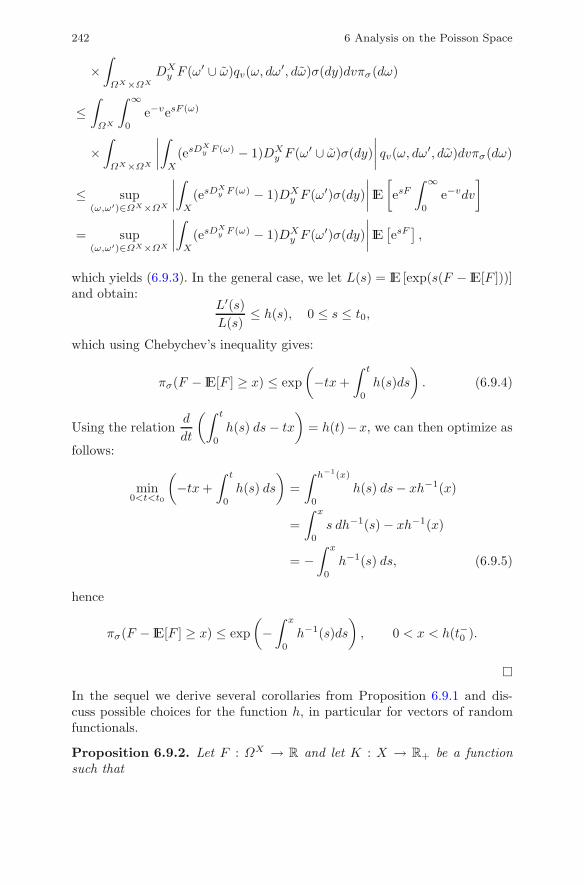
242 6 Analysis on the Poisson Space
×∫
ΩX×ΩX
DXy F (ω′ ∪ ω)qv(ω, dω′, dω)σ(dy)dvπσ(dω)
≤∫
ΩX
∫ ∞
0
e−vesF (ω)
×∫
ΩX×ΩX
∣∣∣∣∫
X
(esDXy F (ω) − 1)DX
y F (ω′ ∪ ω)σ(dy)∣∣∣∣ qv(ω, dω′, dω)dvπσ(dω)
≤ sup(ω,ω′)∈ΩX×ΩX
∣∣∣∣∫
X
(esDXy F (ω) − 1)DX
y F (ω′)σ(dy)∣∣∣∣ IE
[esF
∫ ∞
0
e−vdv
]
= sup(ω,ω′)∈ΩX×ΩX
∣∣∣∣∫
X
(esDXy F (ω) − 1)DX
y F (ω′)σ(dy)∣∣∣∣ IE
[esF
],
which yields (6.9.3). In the general case, we let L(s) = IE [exp(s(F − IE[F ]))]and obtain:
L′(s)L(s)
≤ h(s), 0 ≤ s ≤ t0,
which using Chebychev’s inequality gives:
πσ(F − IE[F ] ≥ x) ≤ exp(−tx+
∫ t
0
h(s)ds). (6.9.4)
Using the relationd
dt
(∫ t
0
h(s) ds− tx
)= h(t)−x, we can then optimize as
follows:
min0<t<t0
(−tx+
∫ t
0
h(s) ds)
=∫ h−1(x)
0
h(s) ds− xh−1(x)
=∫ x
0
s dh−1(s) − xh−1(x)
= −∫ x
0
h−1(s) ds, (6.9.5)
hence
πσ(F − IE[F ] ≥ x) ≤ exp(−∫ x
0
h−1(s)ds), 0 < x < h(t−0 ).
�In the sequel we derive several corollaries from Proposition 6.9.1 and dis-cuss possible choices for the function h, in particular for vectors of randomfunctionals.
Proposition 6.9.2. Let F : ΩX → R and let K : X → R+ be a functionsuch that

6.9 Deviation Inequalities 243
DXy F (ω) ≤ K(y), y ∈ X, ω ∈ ΩX . (6.9.6)
Then
πσ(F − IE[F ] ≥ x) ≤ exp(
mint>0
(−tx+
∫ t
0
h(s) ds))
, x > 0,
where
h(t) = supω∈ΩX
∫
X
etK(y) − 1K(y)
|DXy F (ω)|2σ(dy), t > 0. (6.9.7)
If moreover h is finite on [0, t0) then
πσ(F − IE[F ] ≥ x) ≤ exp(−∫ x
0
h−1(s)ds), 0 < x < h(t−0 ). (6.9.8)
If K(y) = 0, y ∈ X, we have:
πσ(F − IE[F ] ≥ x) ≤ exp(− x2
2α2
), x > 0,
with
α2 = supω∈ΩX
∫
X
(DXy F (ω))2σ(dy).
Proof. Let Fn = max(−n,min(F, n)), n ≥ 1. Since when K is R+-valuedthe condition DX
y Fn(ω) ≤ K(y), ω ∈ ΩX , y ∈ X , is satisfied we may applyProposition 6.9.1 to Fn to get
h(t) = sup(ω,ω′)∈ΩX×ΩX
∣∣∣∣∣
∫
X
etDXy Fn(ω) − 1DX
y Fn(ω)DX
y Fn(ω)DXy Fn(ω′) σ(dy)
∣∣∣∣∣
≤ sup(ω,ω′)∈ΩX×ΩX
∫
X
etK(y) − 1K(y)
|DXy Fn(ω)| |DX
y Fn(ω′)| σ(dy)
≤ 12
sup(ω,ω′)∈ΩX×ΩX
∫
X
etK(y) − 1K(y)
(|DXy Fn(ω)|2 + |DX
y Fn(ω′)|2) σ(dy)
≤ supω∈ΩX
∫
X
etK(y) − 1K(y)
|DXy Fn(ω)|2 σ(dy)
≤ supω∈ΩX
∫
X
etK(y) − 1K(y)
|DXy F (ω)|2 σ(dy),
from which the conclusion follows after letting n tend to infinity. �
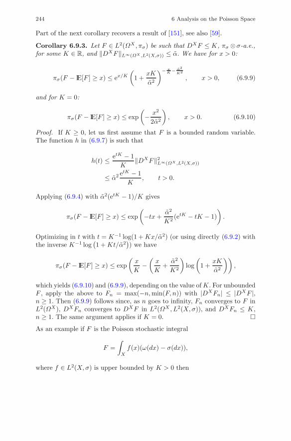
244 6 Analysis on the Poisson Space
Part of the next corollary recovers a result of [151], see also [59].
Corollary 6.9.3. Let F ∈ L2(ΩX , πσ) be such that DXF ≤ K, πσ ⊗ σ-a.e.,for some K ∈ R, and ‖DXF‖L∞(ΩX ,L2(X,σ)) ≤ α. We have for x > 0:
πσ(F − IE[F ] ≥ x) ≤ ex/K
(1 +
xK
α2
)− xK− α2
K2
, x > 0, (6.9.9)
and for K = 0:
πσ(F − IE[F ] ≥ x) ≤ exp(− x2
2α2
), x > 0. (6.9.10)
Proof. If K ≥ 0, let us first assume that F is a bounded random variable.The function h in (6.9.7) is such that
h(t) ≤ etK − 1K
‖DXF‖2L∞(ΩX ,L2(X,σ))
≤ α2 etK − 1K
, t > 0.
Applying (6.9.4) with α2(etK − 1)/K gives
πσ(F − IE[F ] ≥ x) ≤ exp(−tx+
α2
K2(etK − tK − 1)
).
Optimizing in t with t = K−1 log(1 +Kx/α2) (or using directly (6.9.2) withthe inverse K−1 log
(1 +Kt/α2
)) we have
πσ(F − IE[F ] ≥ x) ≤ exp(x
K−(x
K+α2
K2
)log
(1 +
xK
α2
)),
which yields (6.9.10) and (6.9.9), depending on the value ofK. For unboundedF , apply the above to Fn = max(−n,min(F, n)) with |DXFn| ≤ |DXF |,n ≥ 1. Then (6.9.9) follows since, as n goes to infinity, Fn converges to F inL2(ΩX), DXFn converges to DXF in L2(ΩX , L2(X,σ)), and DXFn ≤ K,n ≥ 1. The same argument applies if K = 0. �As an example if F is the Poisson stochastic integral
F =∫
X
f(x)(ω(dx) − σ(dx)),
where f ∈ L2(X,σ) is upper bounded by K > 0 then

6.10 Notes and References 245
πσ(F − IE[F ] ≥ x) ≤ ex/K
(1 +
xK
α2
)− xK− α2
K2
, x > 0,
whereα2 =
∫
X
|f(x)|2σ(dx).
Corollary 6.9.3 yields the following result which recovers Corollary 1 of [55].
Corollary 6.9.4. Let
F = (F1, . . . , Fn) =
(∫
{|y|2≤1}yk (ω(dy) − σ(dy))+
∫
{|y|2>1}yk ω(dy)
)
1≤k≤n
(6.9.11)be an infinitely divisible random variable in R
n with Levy measure σ. Assumethat X = R
n and σ(dx) has bounded support, let
K = inf{r > 0 : σ({x ∈ X : ‖x‖ > r}) = 0},
and α2 =∫
Rn ‖y‖2σ(dy). For any Lipschitz (c) function f : Rn → R with
respect to a given norm ‖ · ‖ on Rn, we have
πσ(f(F ) − IE[f(F )] ≥ x) ≤ ex/(cK)
(1 +
xK
cα2
)−x/(cK)−α2/K2
, x > 0.
Proof. The representation (6.9.11) shows that
|DXx f(F )(ω)| = |f(F (ω ∪ {x})) − f(F (ω))|
≤ c‖F (ω ∪ {x}) − F (ω)‖= c‖x‖. (6.9.12)
We conclude the proof by an application of Corollary 6.9.3. �
6.10 Notes and References
Early statements of the Clark formula on the Poisson space can be found in[129], [130] and [131]. See also [1] for a white noise version of this formulaon Poisson space. The Clark formula for Levy processes has been consideredin [1], [108], [98], [137], and applied to quadratic hedging in incomplete mar-kets driven by jump processes in [98]. The construction of stochastic analysison the Poisson space using difference operators has been developed in [66],[33], [95], [100], cf. [94] for the Definition 6.2.3 of Poisson multiple stochas-tic integrals. The Kabanov [68] multiplication formula has been extended to

246 6 Analysis on the Poisson Space
Azema martingales in [116]. Symmetric difference operators on the Poissonspace have also been introduced in [100]. The study of the characterization ofPoisson measures by integration by parts has been initiated in [86], see also[123], Relation (6.4.12) is also known as the Mecke characterization of Poissonmeasures. Proposition 6.5.5 is useful to study the invariance of Poisson mea-sures under random transformations, cf. [114]. The deviation inequalitiespresented in this chapter are based on [21]. On the Poisson space, explicitcomputations of chaos expansions can be carried out from Proposition 4.2.5(cf. [66] and [138]) using the iterated difference operator DX
t1 · · ·DXtnF , but
may be complicated by the recursive computation of finite differences, cf. [79].A direct calculation using only the operator D can also be found in [80], fora Poisson process on a bounded interval, see also [110] for the chaos decom-position of Proposition 6.3.4. See [99] for a characterization of anticipativeintegrals with respect to the compensated Poisson process.

Chapter 7
Local Gradients on the Poisson Space
We study a class of local gradient operators on Poisson space that havethe derivation property. This allows us to give another example of a gra-dient operator that satisfies the hypotheses of Chapter 3, this time for adiscontinuous process. In particular we obtain an anticipative extension ofthe compensated Poisson stochastic integral and other expressions for theClark predictable representation formula. The fact that the gradient oper-ator satisfies the chain rule of derivation has important consequences fordeviation inequalities, computation of chaos expansions, characterizations ofPoisson measures, and sensitivity analysis. It also leads to the definition ofan infinite dimensional geometry under Poisson measures.
7.1 Intrinsic Gradient on Configuration Spaces
Let X be a Riemannian manifold with volume element σ, cf. e.g. [14]. Wedenote by TxX the tangent space at x ∈ X , and let
TX =⋃
x∈X
TxX
denote the tangent bundle to X . Assume we are given a differential operatorL defined on C1
c (X) with adjoint L∗, satisfying the duality relation
〈Lu, V 〉L2(X,σ;TX) = 〈u, L∗V 〉L2(X,σ), u ∈ C1c (X), V ∈ C1
c (X,TX).
In the sequel, L will be mainly chosen equal to the gradient ∇X on X .We work on the Poisson probability space (ΩX ,FX , πX
σ ) introduced inDefinition 6.1.2.
Definition 7.1.1. Given Λ a compact subset of X, we let S denote the setof functionals F of the form
F (ω) = f01{ω(Λ)=0} +∞∑
n=1
1{ω(Λ)=n}fn(x1, . . . , xn), (7.1.1)
N. Privault, Stochastic Analysis in Discrete and Continuous Settings,Lecture Notes in Mathematics 1982, DOI 10.1007/978-3-642-02380-4 7,c© Springer-Verlag Berlin Heidelberg 2009
247

248 7 Local Gradients on the Poisson Space
where fn ∈ C1c (Λn) is symmetric in n variables, n ≥ 1, with the notation
ω ∩ Λ = {x1, . . . , xn}
when ω(Λ) = n, ω ∈ ΩX .
In the next definition the differential operator L on X is “lifted” to a differ-ential operator DL on ΩX .
Definition 7.1.2. The intrinsic gradient DL is defined on F ∈ S of the form(7.1.1) as
DLxF (ω) =
∞∑
n=1
1{ω(Λ)=n}n∑
i=1
Lxifn(x1, . . . , xn)1{xi}(x), ω(dx) − a.e.,
ω ∈ ΩX .
In other words if ω(Λ) = n and ω ∩ Λ = {x1, . . . , xn} we have
DLxF =
⎧⎨
⎩
Lxifn(x1, . . . , xn), if x = xi for some i ∈ {1, . . . , n},
0, if x /∈ {x1, . . . , xn}.
Let I denote the space of functionals of the form
I ={f
(∫
X
ϕ1(x)ω(dx), . . . ,∫
X
ϕn(x)ω(dx)),
ϕ1, . . . , ϕn ∈ C∞c (X), f ∈ C∞b (Rn), n ∈ N} ,
and
U =
{n∑
i=1
Fiui : u1, . . . , un ∈ C∞c (X), F1, . . . , Fn ∈ I, n ≥ 1
},
Note that for F ∈ I of the form
F = f
(∫
X
ϕ1dω, . . . ,
∫
X
ϕndω
), ϕ1, . . . , ϕn ∈ C∞c (X),
we have
DLxF (ω) =
n∑
i=1
∂if
(∫
X
ϕ1dω, . . . ,
∫
X
ϕndω
)Lxϕi(x), x ∈ ω.
The following result is the integration by parts formula satisfied by DL.
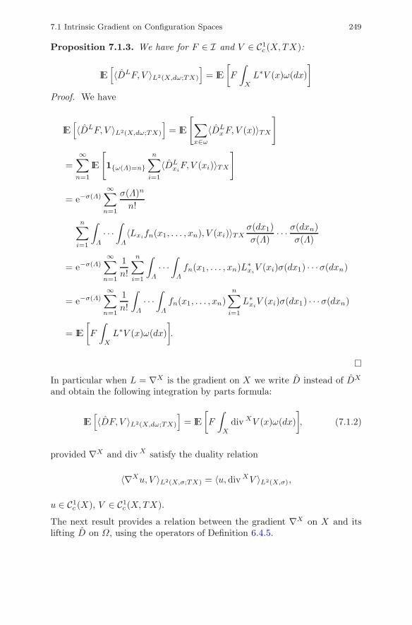
7.1 Intrinsic Gradient on Configuration Spaces 249
Proposition 7.1.3. We have for F ∈ I and V ∈ C1c (X,TX):
IE[〈DLF, V 〉L2(X,dω;TX)
]= IE
[F
∫
X
L∗V (x)ω(dx)]
Proof. We have
IE[〈DLF, V 〉L2(X,dω;TX)
]= IE
[∑
x∈ω
〈DLxF, V (x)〉TX
]
=∞∑
n=1
IE
[1{ω(Λ)=n}
n∑
i=1
〈DLxiF, V (xi)〉TX
]
= e−σ(Λ)∞∑
n=1
σ(Λ)n
n!
n∑
i=1
∫
Λ
· · ·∫
Λ
〈Lxifn(x1, . . . , xn), V (xi)〉TXσ(dx1)σ(Λ)
· · · σ(dxn)σ(Λ)
= e−σ(Λ)∞∑
n=1
1n!
n∑
i=1
∫
Λ
· · ·∫
Λ
fn(x1, . . . , xn)L∗xiV (xi)σ(dx1) · · ·σ(dxn)
= e−σ(Λ)∞∑
n=1
1n!
∫
Λ
· · ·∫
Λ
fn(x1, . . . , xn)n∑
i=1
L∗xiV (xi)σ(dx1) · · ·σ(dxn)
= IE[F
∫
X
L∗V (x)ω(dx)].
�In particular when L = ∇X is the gradient on X we write D instead of DX
and obtain the following integration by parts formula:
IE[〈DF, V 〉L2(X,dω;TX)
]= IE
[F
∫
X
div XV (x)ω(dx)], (7.1.2)
provided ∇X and div X satisfy the duality relation
〈∇Xu, V 〉L2(X,σ;TX) = 〈u, div XV 〉L2(X,σ),
u ∈ C1c (X), V ∈ C1
c (X,TX).
The next result provides a relation between the gradient ∇X on X and itslifting D on Ω, using the operators of Definition 6.4.5.

250 7 Local Gradients on the Poisson Space
Lemma 7.1.4. For F ∈ I we have
DxF (ω) = ε−x ∇Xε+x F (ω) on {(ω, x) ∈ Ωx ×X : x ∈ ω}. (7.1.3)
Proof. Let
F = f
(∫
X
ϕ1dω, . . . ,
∫
X
ϕndω
), x ∈ X, ω ∈ ΩX ,
and assume that x ∈ ω. We have
DxF (ω) =n∑
i=1
∂if
(∫
X
ϕ1dω, . . . ,
∫
X
ϕndω
)∇Xϕi(x)
=n∑
i=1
∂if
(ϕ1(x) +
∫
X
ϕ1d(ω\x), . . . , ϕn(x) +∫
X
ϕnd(ω\x))∇Xϕi(x)
= ∇Xf
(ϕ1(x) +
∫
X
ϕ1d(ω\x), . . . , ϕn(x) +∫
X
ϕnd(ω\x))
= ∇Xε+x f
(∫
X
ϕ1d(ω\x), . . . ,∫
X
ϕnd(ω\x))
=(∇Xε+x F
)(ω\{x})
= ε−x ∇Xε+x F (ω).
�The next proposition uses the operator δX defined in Definition 6.4.1.
Proposition 7.1.5. For V ∈ C∞c (X ;TX) and F ∈ I we have
〈DF (ω), V 〉L2(X,dω;TX) (7.1.4)
= 〈∇XDF (ω), V 〉L2(X,σ;TX) + δX(〈∇XDF, V 〉TX)(ω).
Proof. This identity follows from the relation
DxF (ω) = (∇Xx DxF )(ω\{x}), x ∈ ω,
and the application to u = 〈∇XDF, V 〉TX of the relation
δX(u) =∫
X
u(x, ω\{x})ω(dx) −∫
X
u(x, ω)σ(dx),
cf. Relation (6.5.2) in Proposition 6.5.2. �In addition, for F,G ∈ I we have the isometry
〈DF, DG〉L2ω(TX) = 〈ε−∇Xε+F, ε−∇Xε+G〉L2
ω(TX), (7.1.5)

7.1 Intrinsic Gradient on Configuration Spaces 251
ω ∈ ΩX , as an application of Relation (7.1.3) that holds ω(dx)-a.e. for fixedω ∈ ΩX .Similarly from (7.1.5) and Proposition 6.5.2 we have the relation
〈DF, DG〉L2ω(TX) = δX
(〈∇XDF,∇XDG〉TX
)+ 〈∇XDF,∇XDG〉L2
σ(TX),(7.1.6)
ω ∈ ΩX , F,G ∈ I. Taking expectations on both sides in (7.1.4) using Relation(6.4.5), we recover Relation (7.1.2) in a different way:
IE[〈DF (ω), V 〉L2(X,dω;TX)] = IE[〈∇XDF, V 〉L2(X,σ;TX)]
= IE[FδX(div XV )],
V ∈ C∞c (X ;TX), F ∈ I.
Definition 7.1.6. Let δπσ denote the adjoint of D under πσ, defined as
IEπσ
[F δπσ(G)
]= IEπσ
[〈DF, DG〉L2
ω(TX)
],
on G ∈ I such that
I � F → IEπσ
[〈DF, DG〉L2
ω(TX)
]
extends to a bounded operator on L2(ΩX , πσ).
We close this section with a remark on integration by parts characterizationof Poisson measures, cf. Section 6.6, using the local gradient operator insteadof the finite difference operator. We now assume that div X
σ is defined on ∇Xffor all f ∈ C∞c (X), with
∫
X
g(x)div Xσ ∇Xf(x)σ(dx) =
∫
X
〈∇Xg(x),∇Xf(x)〉TxXσ(dx),
f, g ∈ C1c (X).
As a corollary of our pointwise lifting of gradients we obtain in particular acharacterization of the Poisson measure. Let
HXσ = div X
σ ∇X
denote the Laplace-Beltrami operator on X .
Corollary 7.1.7. The isometry relation
IEπ
[〈DF, DG〉L2
ω(TX)
]= IEπ
[〈∇XDF,∇XDG〉L2σ(TX)
], (7.1.7)
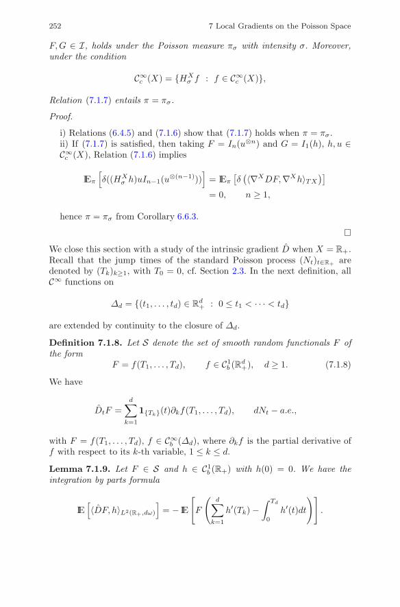
252 7 Local Gradients on the Poisson Space
F,G ∈ I, holds under the Poisson measure πσ with intensity σ. Moreover,under the condition
C∞c (X) = {HXσ f : f ∈ C∞c (X)},
Relation (7.1.7) entails π = πσ.
Proof.
i) Relations (6.4.5) and (7.1.6) show that (7.1.7) holds when π = πσ.ii) If (7.1.7) is satisfied, then taking F = In(u⊗n) and G = I1(h), h, u ∈C∞c (X), Relation (7.1.6) implies
IEπ
[δ((HX
σ h)uIn−1(u⊗(n−1)))]
= IEπ
[δ(〈∇XDF,∇Xh〉TX
)]
= 0, n ≥ 1,
hence π = πσ from Corollary 6.6.3.
�We close this section with a study of the intrinsic gradient D when X = R+.Recall that the jump times of the standard Poisson process (Nt)t∈R+ aredenoted by (Tk)k≥1, with T0 = 0, cf. Section 2.3. In the next definition, allC∞ functions on
Δd = {(t1, . . . , td) ∈ Rd+ : 0 ≤ t1 < · · · < td}
are extended by continuity to the closure of Δd.
Definition 7.1.8. Let S denote the set of smooth random functionals F ofthe form
F = f(T1, . . . , Td), f ∈ C1b (Rd
+), d ≥ 1. (7.1.8)
We have
DtF =d∑
k=1
1{Tk}(t)∂kf(T1, . . . , Td), dNt − a.e.,
with F = f(T1, . . . , Td), f ∈ C∞b (Δd), where ∂kf is the partial derivative off with respect to its k-th variable, 1 ≤ k ≤ d.
Lemma 7.1.9. Let F ∈ S and h ∈ C1b (R+) with h(0) = 0. We have the
integration by parts formula
IE[〈DF, h〉L2(R+,dω)
]= − IE
[F
(d∑
k=1
h′(Tk) −∫ Td
0
h′(t)dt
)].

7.1 Intrinsic Gradient on Configuration Spaces 253
Proof. By integration by parts on Δd using Relation (2.3.4) we have, forF ∈ S of the form (7.1.8),
IE[〈DF, h〉L2(R+,dNt)] =d∑
k=1
∫ ∞
0
∫ td
0
· · ·∫ t2
0
e−td h(tk)∂kf(t1, . . . , td)dt1 · · · dtd
=
∫ ∞
0
e−td
∫ td
0
· · ·∫ t2
0
h(t1)∂1f(t1, . . . , td)dt1 · · · dtd
+d∑
k=2
∫ ∞
0
e−td
∫ td
0
· · ·∫ tk+1
0
h(tk)∂
∂tk
∫ tk
0
· · ·∫ t2
0
f(t1, . . . , td)dt1 · · · dtd
−d∑
k=2
∫ ∞
0
e−td
∫ td
0
·∫ tk+1
0
h(tk)
∫ tk
0
∫ tk−2
0
·∫ t2
0
f(t1, . . . , tk−2, tk, tk, . . . , td)dt1 · dtk−1 · dtd
= −∫ ∞
0
e−td
∫ td
0
· · ·∫ t2
0
h′(t1)f(t1, . . . , td)dt1 · · · dtd
+
∫ ∞
0
e−td
∫ td
0
· · ·∫ t3
0
h(t2)f(t2, t2, . . . , td)dt2 · · · dtd
−d∑
k=2
∫ ∞
0
e−td
∫ td
0
·∫ tk+1
0
h′(tk)
∫ tk
0
· · ·∫ t2
0
f(t1, . . . , td)dt1 · · · dtd
+
∫ ∞
0
e−td h(td)
∫ td
0
· · ·∫ t2
0
f(t1, . . . , td)dt1 · · · dtd
+d−1∑
k=2
∫ ∞
0
e−td
∫ td
0
·∫ tk+2
0
h(tk+1)
∫ tk+1
0
∫ tk−1
0
·∫ t2
0
f(t1, ., tk−1, tk+1, tk+1, ., td)dt1 · dtk · dtd
−d∑
k=2
∫ ∞
0
e−td
∫ td
0
·∫ tk+1
0
h(tk)
∫ tk
0
∫ tk−2
0
·∫ t2
0
f(t1, ., tk−2, tk, tk, ., td)dt1 · dtd
= −d∑
k=1
∫ ∞
0
e−td
∫ td
0
· · ·∫ tk+1
0
h′(tk)
∫ tk
0
· · ·∫ t2
0
f(t1, . . . , td)dt1 · · · dtd
+
∫ ∞
0
e−td h(td)
∫ td
0
· · ·∫ t2
0
f(t1, . . . , td)dt1 · · · dtd
= − IE
[F
(d∑
k=1
h′(Tk) −∫ Td
0
h′(t)dt
)],
where dtk denotes the absence of dtk in the multiple integrals with respectto dt1 · · ·dtd. �As a consequence we have the following corollary which directly involves thecompensated Poisson stochastic integral.

254 7 Local Gradients on the Poisson Space
Corollary 7.1.10. Let F ∈ S and h ∈ C1b (R+) with h(0) = 0. We have the
integration by parts formula
IE[〈DF, h〉L2(R+,dω)] = − IE[F
∫ ∞
0
h′(t)d(Nt − t)]. (7.1.9)
Proof. From Lemma 7.1.9 it suffices to notice that if k > d,
IE[Fh′(Tk)] =∫ ∞
0
e−tkh′(tk)∫ tk
0
· · ·∫ td
0
· · ·∫ t2
0
f(t1, . . . , td)dt1 · · · dtk
=∫ ∞
0
e−tkh(tk)∫ tk
0
· · ·∫ td
0
· · ·∫ t2
0
f(t1, . . . , td)dt1 · · · dtk
−∫ ∞
0
e−tk−1h(tk−1)∫ tk−1
0
· · ·∫ td
0
· · ·∫ t2
0
f(t1, . . . , td)dt1 · · · dtk−1
= IE[F (h(Tk) − h(Tk−1))]
= IE
[F
∫ Tk
Tk−1
h′(t)dt
],
in other terms the discrete-time process
(n∑
k=1
h′(Tk) −∫ Tk
0
h′(t)dt
)
k≥1
=
(∫ Tk
0
h′(t)d(Nt − t)
)
k≥1
is a martingale. �Alternatively we may also use the strong Markov property to show directlythat
IE
[F
( ∞∑
k=d+1
h′(Tk) −∫ ∞
Td+1
h′(s)ds
)]= 0.
By linearity the adjoint δ of D is defined on simple processes u ∈ U of theform u = hG, G ∈ S, h ∈ C1(R+), from the relation
δ(hG) = −G∫ ∞
0
h′(t)d(Nt − t) + 〈h, DG〉L2(R+,dNt).
Relation (7.1.9) implies immediately the following duality relation.
Proposition 7.1.11. For F ∈ S and h ∈ C1c (R+) we have :
IE[〈DF, hG〉L2(R+,dNt)
]= IE
[F δ(hG)
].

7.2 Damped Gradient on the Half Line 255
Proof. We have
IE[〈DF, hG〉L2(R+,dNt)
]= IE
[〈D(FG), h〉L2(R+,dNt) − F 〈DG, h〉L2(R+,dNt)
]
= IE[F (Gδ(h) − 〈h, DG〉L2(R+,dNt))
]
= − IE[F
(G
∫ ∞
0
h′(t)d(Nt − t) + 〈h, DG〉L2(R+,dNt)
)]
= IE[F δ(hG)
].
�
7.2 Damped Gradient on the Half Line
In this section we construct an example of a gradient which, has the derivationproperty and, unlike D, satisfies the duality Assumption 3.1.1 and the Clarkformula Assumption 3.2.1 of Section 3.1. Recall that the jump times of thestandard Poisson process (Nt)t∈R+ are denoted by (Tk)k≥1, with T0 = 0, cf.Section 2.3.Let
r(t, s) = −(s ∨ t), s, t ∈ R+,
denote the Green function associated to equation
⎧⎨
⎩
Lf := −f ′′, f ∈ C∞([0,∞))
f ′(0) = f ′(∞) = 0.
In other terms, given g ∈ C∞([0,∞)), the solution of
g(t) = −f ′′(t), f ′(0) = f ′(∞) = 0,
is given by
f(t) =∫ ∞
0
r(t, s)g(s)ds, t ∈ R+.
Let also
r(1)(t, s) =∂r
∂t(t, s)
= −1]−∞,t](s), s, t ∈ R+,

256 7 Local Gradients on the Poisson Space
i.e.
f(t) =∫ ∞
0
r(1)(t, s)g(s)ds
= −∫ t
0
g(s)ds, t ∈ R+, (7.2.1)
is the solution of ⎧⎨
⎩
f ′ = −g,
f(0) = 0.
Let S denote the space of functionals of the form
I ={F = f(T1, . . . , Td) : f ∈ C1
b (Rd), d ≥ 1},
and let
U =
{n∑
i=1
Fiui : u1, . . . , un ∈ Cc(R+), F1, . . . , Fn ∈ S, n ≥ 1
}.
Definition 7.2.1. Given F ∈ S of the form F = f(T1, . . . , Td), we let
DsF = −d∑
k=1
1[0,Tk](s)∂kf(T1, . . . , Td).
Note that we have
DsF =d∑
k=1
r(1)(Tk, s)∂kf(T1, . . . , Td)
=∫ ∞
0
r(1)(t, s)DtFdNt.
From Proposition 2.3.6 we have the following lemma.
Lemma 7.2.2. For F of the form F = f(T1, . . . , Tn) we have
IE[DtF |Ft] = −∑
Nt<k≤n
IE[∂kf(T1, . . . , Tn)|Ft]
= −∑
Nt<k≤n
∫ ∞
t
e−(sn−t)
∫ sn
t
· · ·∫ sNt+2
t
∂kf(T1, . . . , TNt, sNt+1, . . . , sn)dsNt+1 · · ·dsn.

7.2 Damped Gradient on the Half Line 257
According to Definition 3.2.2, ID([a,∞)), a > 0, denotes the completion of Sunder the norm
‖F‖ID([a,∞)) = ‖F‖L2(Ω) +(
IE[∫ ∞
a
|DtF |2dt])1/2
,
i.e. (DtF )t∈[a,∞) is defined in L2(Ω× [a,∞)) for F ∈ ID([a,∞)). Clearly, thestability Assumption 3.2.10 is satisfied by D since
1[0,Tk](t) = 1{Nt<k}
is Ft-measurable, t ∈ R+, k ∈ N. Hence the following lemma holds as a con-sequence of Proposition 3.2.11. For completeness we provide an independentdirect proof.
Lemma 7.2.3. Let T > 0. For any FT -measurable random variable F ∈L2(Ω) we have F ∈ ID[T,∞) and
DtF = 0, t ≥ T.
Proof. In case F = f(T1, . . . , Tn) with f ∈ C∞c (Rn), F does not depend onthe future of the Poisson process after T , it does not depend on the k-thjump time Tk if Tk > T , i.e.
∂if(T1, . . . , Tn) = 0 for Tk > T, 1 ≤ k ≤ i ≤ n.
This implies
∂if(T1, . . . , Tn)1[0,Ti](t) = 0 t ≥ T i = 1, . . . , n,
and
DtF = −n∑
i=1
∂if(T1, . . . , Tn)1[0,Ti](t) = 0 t ≥ T.
Hence DtF = 0, t ≥ T . �
Proposition 7.2.4. We have for F ∈ S and u ∈ Cc(R+):
IE[〈DF, u〉L2(R+,dt)] = IE[F
∫ ∞
0
u(t)(dNt − dt)]. (7.2.2)
Proof. We have, using (7.2.1),
IE[〈DF, u〉L2(R+,dt)
]= IE
[∫ ∞
0
∫ ∞
0
r(1)(s, t)DsFu(t)dNsdt
]

258 7 Local Gradients on the Poisson Space
= − IE
[⟨D·F,
∫ ·
0
u(t)dt⟩
L2(R+,dNt)
]
= IE[F
∫ ∞
0
u(t)d(Nt − t)],
from Corollary 7.1.10. �The above proposition can also be proved by finite dimensional integrationby parts on jump times conditionally to the value of NT , see Proposition 7.3.3below.The divergence operator defined next is the adjoint of D.
Definition 7.2.5. We define δ on U by
δ(hG) = G
∫ ∞
0
h(t)(dNt − dt) − 〈h, DG〉L2(R+),
G ∈ S, h ∈ L2(R+).
The closable adjoint
δ : L2(Ω × [0, 1]) −→ L2(Ω)
of D is another example of a Skorokhod type integral on the Poisson space.Using this definition we obtain the following integration by parts formulawhich shows that the duality Assumption 3.1.1 is satisfies by D and δ.
Proposition 7.2.6. The divergence operator
δ : L2(Ω × R+) −→ L2(Ω)
is the adjoint of the gradient operator
D : L2(Ω) → L2(Ω × R+),
i.e. we have
IE[F δ(u)
]= IE
[〈DF, u〉L2(R+)
], F ∈ S, u ∈ U . (7.2.3)
Proof. It suffices to note that Proposition 7.2.4 implies
IE[〈DF, hG〉L2(R+,dt)] = IE[〈D(FG), h〉L2(R+,dt) − F 〈DG, h〉L2(R+,dt)
]
= IE[F
(G
∫ ∞
0
h(t)d(Nt − t) − 〈h, DG〉L2(R+,dt)
)],
(7.2.4)
for F,G ∈ S. �

7.2 Damped Gradient on the Half Line 259
As a consequence, the duality Assumption 3.1.1 of Section 3 is satisfied byD and δ and from Proposition 3.1.2 we deduce that D and δ are closable.Recall that from Proposition 6.4.9, the finite difference operator
DtF = 1{Nt<n}(f(T1, . . . , TNt , t, TNt+1, . . . , Tn−1) − f(T1, . . . , Tn)),
t ∈ R+, F = f(T1, . . . , Tn), defined in Chapter 6 satisfies the Clark formulaAssumption 3.2.1, i.e. by Proposition 4.2.3 applied to φt = 1, t ∈ R+, wehave
F = IE[F ] +∫ ∞
0
IE[DtF | Ft]d(Nt − t), (7.2.5)
F ∈ L2(Ω).
On the other hand, the gradient D has the derivation property and for thisreason it can be easier to manipulate than the finite difference operator D inrecursive computations. Its drawback is that its domain is smaller than thatof D, due to the differentiability conditions it imposes on random functionals.In the next proposition we show that the adapted projections of (DtF )t∈R+
and (DtF )t∈R+ coincide, cf. e.g. Proposition 20 of [102], by a direct compu-tation of conditional expectations.
Proposition 7.2.7. The adapted projections of D and D coincide, i.e.
IE[DtF | Ft] = IE[DtF | Ft], t ∈ R+.
Proof. We have
IE[DtF |Ft] = −n∑
k=1
1[0,Tk](t) IE[∂kf(T1, . . . , Tn)|Ft]
= −∑
Nt<k≤n
IE[∂kf(T1, . . . , Tn)|Ft]
= −∑
Nt<k≤n∫ ∞
0
e−(sn−t)∫ sn
t
· · ·∫ sNt+2
t
∂kf(T1, . . . , TNt , sNt+1, . . . , sn)dsNt+1 · · · dsn
= −n∑
k=Nt+2
∫ ∞
t
e−(sn−t)∫ sn
t
· · ·
· · · ∂
∂sk
∫ sk
t
· · ·∫ sNt+2
t
f(T1, . . . , TNt , sNt+1, . . . , sn)dsNt+1 · · · dsn
+n∑
k=Nt+2
∫ ∞
t
e−(sn−t)∫ sn
t
· · ·
· · ·∫ sNt+2
t
f(T1, . . . , TNt , sNt+1, ., sk−2, sk, sk, sk+1, ., sn)
dsNt+1 · · · dsk−1 · · · dsn

260 7 Local Gradients on the Poisson Space
−1{n>Nt}
∫ ∞
t
e−(sn−t)∫ sn
t
· · ·∫ sNt+2
t
∂Nt+1f(T1, . . . , TNt , sNt+1, . . . , sn)
dsNt+1 · · · dsn
= −1{Nt<n−1}
∫ ∞
t
e−(sn−t) ∂
∂sn
∫ sn
t
· · ·∫ sNt+2
t
f(T1, . . . , TNt , sNt+1, . . . , sn)
dsNt+1 · · · dsn
−n−1∑
k=Nt+2
∫ ∞
t
e−(sn−t)∫ sn
t
· · ·
∂
∂sk
∫ sk
t
· · ·∫ sNt+2
t
f(T1, . . . , TNt , sNt+1, . . . , sn)dsNt+1 · · · dsn
+n∑
k=Nt+2
∫ ∞
t
e−(sn−t)∫ sn
t
· · ·∫ sNt+2
t
f(T1, . . . , TNt , sNt+1, ., sk−2, sk, sk, sk+1, ., sn)dsNt+1 · · · dsk−1 · · · dsn
−1{n>Nt}
∫ ∞
t
e−(sn−t)∫ sn
t
· · ·∫ sNt+2
t
∂Nt+1f(T1, . . . , TNt , sNt+1, . . . , sn)
dsNt+1 · · · dsn
= −1{Nt<n−1}
∫ ∞
t
e−(sn−t) ∂
∂sn
∫ sn
t
· · ·∫ sNt+2
t
f(T1, . . . , TNt , sNt+1, . . . , sn)
dsNt+1 · · · dsn
−n−1∑
k=Nt+2
∫ ∞
t
e−(sn−t)∫ sn
t
· · ·∫ sNt+2
t
f(T1, . . . , TNt , sNt+1, . . . , sk−1, sk+1, sk+1, . . . , sn)dsNt+1 · · · dsk · · · dsn
+n∑
k=Nt+2
∫ ∞
t
e−(sn−t)∫ sn
t
· · ·∫ sNt+2
t
f(T1, . . . , TNt , sNt+1, ., sk−2, sk, sk, sk+1, ., sn)dsNt+1 · · · dsk−1 · · · dsn
−1{n>Nt}
∫ ∞
t
e−(sn−t)∫ sn
t
· · ·∫ sNt+2
t
∂Nt+1f(T1, . . . , TNt , sNt+1, . . . , sn)
dsNt+1 · · · dsn
= −1{Nt<n−1}
∫ ∞
t
e−(sn−t)∫ sn
t
· · ·∫ sNt+2
t
f(T1, . . . , TNt , sNt+1, . . . , sn)
dsNt+1 · · · dsn
+1{Nt<n−1}
∫ ∞
t
e−(sn−t)∫ sn
t
· · ·∫ sNt+2
t
f(T1, . . . , TNt , sNt+2, sNt+2, . . . , sn)
dsNt+1 · · · dsn
−1{n>Nt}
∫ ∞
t
e−(sn−t)∫ sn
t
· · ·∫ sNt+2
t
∂Nt+1f(T1, . . . , TNt , sNt+1, . . . , sn)
dsNt+1 · · · dsn
= −1{Nt<n−1}
∫ ∞
0
e−(sn−t)∫ sn
t
· · ·∫ sNt+2
t
f(T1, . . . , TNt , sNt+1, . . . , sn)
dsNt+1 · · · dsn

7.2 Damped Gradient on the Half Line 261
+1{Nt<n−1}
∫ ∞
t
e−(sn−t)∫ sn
t
· · ·∫ sNt+2
t
f(T1, . . . , TNt , sNt+2, sNt+2, . . . , sn)
dsNt+1 · · · dsn
−1{Nt<n−1}
∫ ∞
t
e−(sn−t)∫ sn
t
· · ·∫ sNt+3
t
f(T1, . . . , TNt , sNt+2, sNt+2, . . . , sn)
dsNt+2 · · · dsn
+1{Nt<n−1}
∫ ∞
t
e−(sn−t)∫ sn
t
· · ·∫ sNt+3
t
f(T1, . . . , TNt , t, sNt+2, . . . , sn)
dsNt+2 · · · dsn
−1{n=Nt+1}
∫ ∞
t
e−(sn−t)f(T1, . . . , Tn−1, sn)dsn
+1{n=Nt+1}f(T1, . . . , Tn−1, t)
= −1{n>Nt}
∫ ∞
t
e−(sn−t)∫ sn
t
· · ·∫ sNt+2
t
f(T1, . . . , TNt , sNt+1, . . . , sn)
dsNt+1 · · · dsn
+1{n<Nt}
∫ ∞
t
e−(sn−t)∫ sn
t
· · ·∫ sNt+3
t
f(T1, . . . , TNt , t, sNt+2, . . . , sn)
dsNt+2 · · · dsn
= IE[DtF |Ft],
from Lemma 6.4.10. �As a consequence of Proposition 7.2.7 we also have
IE[DtF | Fa] = IE[DtF | Fa], 0 ≤ a ≤ t. (7.2.6)
For functions of a single jump time, by Relation (2.3.6) we simply have
IE[Dtf(Tn)|Ft] = −1{Nt<n}(t) IE[f ′(Tn)|Ft]
= −1{Nt<n}
(1{Nt≥n}f ′(Tn) +
∫ ∞
t
f ′(x)pn−1−Nt(x− t)dx)
= −∫ ∞
t
f ′(x)pn−1−Nt(x − t)dx
= f(t)pn−1−Nt(0) +∫ ∞
t
f(x)p′n−1−Nt(x − t)dx
= f(t)1{Tn−1<t<Tn} +∫ ∞
t
f(x)p′n−1−Nt(x− t)dx,
which coincides with
IE[Dtf(Tn)|Ft]
= IE[1{Nt<n−1}(f(Tn−1) − f(Tn)) + 1{Nt=n−1}(f(t) − f(Tn))|Ft]
262 7 Local Gradients on the Poisson Space
= IE[(1{Tn−1>t}f(Tn−1) + 1{Tn−1<t<Tn}f(t) − 1{Tn>t}f(Tn))|Ft]
= 1{Tn−1<t<Tn}f(t) + IE[(1{Tn−1>t}f(Tn−1) − 1{Tn>t}f(Tn))|Ft]
= 1{Tn−1<t<Tn}f(t) +∫ ∞
t
(pn−2−Nt(x− t) − pn−1−Nt(x− t))f(x)dx
= 1{Tn−1<t<Tn}f(t) +∫ ∞
t
f(x)p′n−1−Nt(x− t)dx.
As a consequence of Proposition 7.2.7 and (7.2.5) we find that D satisfies theClark formula, hence the Clark formula Assumption 3.2.1 is satisfied by D.
Proposition 7.2.8. For any F ∈ L2(Ω) we have
F = IE[F ] +∫ ∞
0
IE[DtF | Ft]d(Nt − t).
In other words we have
F = IE[F ] +∫ ∞
0
IE[DtF |Ft]d(Nt − t)
= IE[F ] +∫ ∞
0
IE[DtF |Ft]d(Nt − t),
F ∈ L2(Ω).
Since the duality Assumption 3.1.1 and the Clark formula Assumption 3.2.1are satisfied by D, it follows from Proposition 3.3.1 that the operator δcoincides with the compensated Poisson stochastic integral with respect to(Nt − t)t∈R+ on the adapted square-integrable processes. This fact is statedin the next proposition with an independent proof.
Proposition 7.2.9. The adjoint of D extends the compensated Poisson sto-chastic integral, i.e. for all adapted square-integrable process u ∈ L2(Ω×R+)we have
δ(u) =∫ ∞
0
utd(Nt − t).
Proof. We consider first the case where v is a cylindrical elementary pre-dictable process v = F1(s,T ](·) with F = f(T1, . . . , Tn), f ∈ C∞c (Rn). Since vis predictable, F is Fs-measurable hence from Lemma 7.2.3 we have DtF = 0,s ≥ t, and
Dtvu = 0, t ≥ u.

7.3 Damped Gradient on a Compact Interval 263
Hence from Definition 7.2.5 we get
δ(v) = F (NT − Nt)
=∫ ∞
0
F1(t,T ](s)dNs
=∫ ∞
0
vsdNs.
We then use the fact that D is linear to extend the property to the linearcombinations of elementary predictable processes. The compensated Poissonstochastic integral coincides with δ on the predictable square-integrable pro-cesses from a density argument using the Ito isometry. �Since the adjoint δ of D extends the compensated Poisson stochastic integral,we may also use Proposition 3.3.2 to show that the Clark formula Assumption3.2.1 is satisfied by D, and in this way we recover the fact that the adaptedprojections of D and D coincide:
IE[DtF | Ft] = IE[DtF | Ft], t ∈ R+,
for F ∈ L2(Ω).
7.3 Damped Gradient on a Compact Interval
In this section we work under the Poisson measure on the compact interval[0, T ], T > 0.
Definition 7.3.1. We denote by Sc the space of Poisson functionals of theform
F = hn(T1, . . . , Tn), hn ∈ Cc((0,∞)n), n ≥ 1, (7.3.1)
and by Sf the space of Poisson functionals of the form
F = f01{NT =0} +m∑
n=1
1{NT =n}fn(T1, . . . , Tn), (7.3.2)
where f0 ∈ R and fn ∈ C1([0, T ]n), 1 ≤ n ≤ m, is symmetric in n variables,m ≥ 1.
The elements of Sc can be written as
F = f01{NT =0} +∞∑
n=1
1{NT =n}fn(T1, . . . , Tn),
264 7 Local Gradients on the Poisson Space
where f0 ∈ R and fn ∈ C1([0, T ]n), 1 ≤ n ≤ m, is symmetric in n variables,m ≥ 1, with the continuity condition
fn(T1, . . . , Tn) = fn+1(T1, . . . , Tn, T ).
We also let
Uc =
{n∑
i=1
Fiui : u1, . . . , un ∈ C([0, T ]), F1, . . . , Fn ∈ Sc, n ≥ 1
},
and
Uf =
{n∑
i=1
Fiui : u1, . . . , un ∈ C([0, T ]), F1, . . . , Fn ∈ Sf , n ≥ 1
}.
Recall that under P we have, for all F ∈ Sf of the form (7.3.2):
IE[F ] = e−λT f0 + e−λTm∑
n=1
λn
∫ T
0
∫ tn
0
· · ·∫ t2
0
fn(t1, . . . , tn)dt1 · · · dtn.
Definition 7.3.2. Let D be defined on F ∈ Sf of the form (7.3.2) by
DtF = −m∑
n=1
1{NT =n}n∑
k=1
1[0,Tk](t)∂kfn(T1, . . . , Tn).
If F has the form (7.3.1) we have
DtF = −n∑
k=1
1[0,Tk](t)∂kfn(T1, . . . , Tn),
where ∂kfn denotes the partial derivative of fn with respect to its k-th vari-able as in Definition 7.2.1.We define δ on u ∈ Uf by
δ(Fu) = F
∫ T
0
utdNt −∫ ∞
0
utDtFdt, (7.3.3)
F ∈ Sf , u ∈ C([0, T ]).
The following result shows that D and δ also satisfy the duality Assumption3.1.1.Proposition 7.3.3. The operators D and δ satisfy the duality relation
IE[〈DF, u〉] = IE[F δ(u)], (7.3.4)
F ∈ Sf , u ∈ Uf .

7.3 Damped Gradient on a Compact Interval 265
Proof. By standard integration by parts we first prove (7.3.4) when u ∈ C([0, T ]) and F has the form (7.3.2). We have
IE[〈DF, u〉]
= −e−λTm∑
n=1
λn
n!
n∑
k=1
∫ T
0
· · ·∫ T
0
∫ tk
0
u(s)ds∂kfn(t1, . . . , tn)dt1 · · · dtn
= e−λT∞∑
n=1
λn
n!
n∑
k=1
∫ T
0
· · ·∫ T
0
fn(t1, . . . , tn)u(tk)dt1 · · ·dtn
−e−λT∞∑
n=1
λn
(n− 1)!
∫ T
0
u(s)ds∫ T
0
· · ·∫ T
0
fn(t1, . . . , tn−1, T )dt1 · · ·dtn−1.
The continuity condition
fn(t1, . . . , tn−1, T ) = fn−1(t1, . . . , tn−1) (7.3.5)
yields
IE[〈DF, u〉]
= e−λT∞∑
n=1
λn
n!
∫ T
0
· · ·∫ T
0
fn(t1, . . . , tn)n∑
k=1
u(tk)dt1 · · ·dtn
−λe−λT
∫ T
0
u(s)ds∞∑
n=0
λn
n!
∫ T
0
· · ·∫ T
0
fn(t1, . . . , tn)dt1 · · ·dtn
= IE
[F
(NT∑
k=1
u(Tk) − λ
∫ T
0
u(s)ds
)]
= IE
[F
∫ T
0
u(t)dN(t)
].
Next we define δ(uG), G ∈ Sf , by (7.3.3), with for all F ∈ Sf :
IE[G〈DF, u〉] = IE
[〈D(FG), u〉 − F 〈DG, u〉]
= IE
[F
(G
∫ T
0
u(t)dNt − 〈DG, u〉)]
= IE[F δ(uG)
],
which proves (7.3.4). �
266 7 Local Gradients on the Poisson Space
Hence, the duality Assumption 3.1.1 of Section 3 is also satisfied by D andδ, which are closable from Proposition 3.1.2, with domains Dom(D) andDom (δ).The stability Assumption 3.2.10 is also satisfied by D and Lemma 7.2.3 holdsas well as a consequence of Proposition 3.2.11, i.e. for any FT -measurablerandom variable F ∈ L2(Ω) we have
DtF = 0, t ≥ T.
Similarly, δ coincides with the stochastic integral with respect to the com-pensated Poisson process, i.e.
δ(u) =∫ ∞
0
utd(Nt − t),
for all adapted square-integrable process u ∈ L2(Ω × R+), with the sameproof as in Proposition 7.2.9.Consequently, from Proposition 3.3.2 it follows that the Clark formulaAssumption 3.2.1 is satisfied by D, and the adapted projections of D, D,and D coincide:
IE[DtF | Ft] = IE[DtF | Ft]
= IE[DtF | Ft], t ∈ R+,
for F ∈ L2(Ω).
Note that the gradients D and D coincide on a common domain under thecontinuity condition (7.3.5). In case (7.3.5) is not satisfied by F the gradientDF can still be defined in L2(Ω × [0, T ]) on F ∈ Sf while DF exists only indistribution sense due to the presence of the indicator function 1{NT =k} =1{[Tk,Tk+1)}(T ) in (7.3.2).Yet when (7.3.5) does not hold, we still get the integration by parts
IE[〈DF, u〉] = IE
[F
NT∑
k=1
u(Tk)
](7.3.6)
= IE
[F
∫ T
0
u(t)dN(t)
], F ∈ Sf , u ∈ Uf ,
under the additional condition
∫ T
0
u(s)ds = 0. (7.3.7)

7.4 Chaos Expansions 267
However, in this case Proposition 3.1.2 does not apply to extend D by clos-ability from its definition on Sf since the condition (7.3.7) is required in theintegration by parts (7.3.6).
7.4 Chaos Expansions
In this section we review the application of D to the computation of chaosexpansions whenX = R+. As noted above the gradient D has some propertiesin common with D, namely its adapted projection coincides with that of D,and in particular from Proposition 7.2.7 we have
IE[DtF ] = IE[DtF ], t ∈ R+.
In addition, since the operator D has the derivation property it is easier tomanipulate than the finite difference operator D in recursive computations.We aim at applying Proposition 4.2.5 in order to compute the chaosexpansions
F = IE[F ] +∞∑
n=1
In(fn),
withfn(t1, . . . , tn) =
1n!
IE[Dt1 · · · DtnF ],
dt1 · · · dtndP-a.e., n ≥ 1.
However, Proposition 4.2.5 cannot be applied since the gradient D cannot beiterated in L2 due to the non-differentiability of 1[0,Tk](t) in Tk. In particular,an expression such as
IE[Dt1 · · · DtnF ] (7.4.1)
makes a priori no sense and may differ from IE[Dt1 · · ·DtnF ] for n ≥ 2.Note that we have
Dtn · · · Dt1f(Tk) = (−1)n1[0,Tk](tn)f (n)(Tk), 0 < t1 < · · · < tn,
and
IE[Dtn · · · Dt1f(Tk)] = (−1)n IE[1[0,Tk](tn)f (n)(Tk)]
= (−1)n
∫ ∞
tn
f (n)(t)pk−1(t)dt,
0 < t1 < · · · < tn, which differs from
IE[Dtn · · ·Dt1f(Tk)] = −∫ ∞
tn
f(t)P (n)k (t)dt,
268 7 Local Gradients on the Poisson Space
computed in Theorem 1 of [110], where
Pk(t) =∫ t
0
pk−1(s)ds, t ∈ R+,
is the distribution function of Tk, cf. (6.3.5).Hence on the Poisson space Dtn · · · Dt1 , 0 < t1 < · · · < tn, cannot be usedin the L2 sense as Dtn · · ·Dt1 to give the chaos decomposition of a randomvariable. Nevertheless we have the following proposition, see [112] for anapproach to this problem gradient D in distribution sense.
Proposition 7.4.1. For any F ∈∞⋂
n=0
Dom (DnD) we have the chaos
expansion
F = IE[F ] +∞∑
n≥1
In(1Δnfn),
wherefn(t1, . . . , tn) = IE[Dt1 · · ·Dtn−1DtnF ],
0 < t1 < · · · < tn, n ≥ 1.
Proof. We apply Proposition 4.2.5 to DtF , t ∈ R+:
DtF = IE[DtF ] +∞∑
n=1
In(1ΔnIE[DnDtF ]),
which yields
IE[DtF |Ft] = IE[DtF ] +∞∑
n=1
In(1Δn+1(∗,t) IE[DnDtF ]).
Finally, integrating both sides with respect to d(Nt − t) and using of theClark formula Proposition 7.2.8 and the inductive definition (2.7.1) we get
F − IE[F ] =∞∑
n=0
In+1(1Δn+1IE[DnDF ]).
�The next lemma provides a way to compute the functions appearing inProposition 7.4.1.
Lemma 7.4.2. We have for f ∈ C1c (R) and n ≥ 1
DtDsf(Tn) = Ds∨tf(Tn−1) − Ds∨tf(Tn) − 1{s<t}1[Tn−1,Tn](s ∨ t)f ′(s ∨ t),
s, t ∈ R+.

7.4 Chaos Expansions 269
Proof. From Relation (6.4.15) we have
DtDsf(Tn) = −1[0,Tn−1](t)(1[0,Tn−1](s)f
′(Tn−1) − 1[0,Tn](s)f ′(Tn))
−1[Tn−1,Tn](t)(1[0,t](s)f ′(t) − 1[0,Tn](s)f ′(Tn)
)
= 1{t<s}(1[0,Tn](s)f ′(Tn) − 1[0,Tn−1](s)f
′(Tn−1),)
+1{s<t}(1[0,Tn](t)f ′(Tn) − 1[0,Tn−1](t)f
′(Tn−1) − 1[Tn−1,Tn](t)f ′(t)),
P-a.s. �In the next proposition we apply Lemma 7.4.2 to the computation of thechaos expansion of f(Tk).
Proposition 7.4.3. For k ≥ 1, the chaos expansion of f(Tk) is given as
f(Tk) = IE[f(Tk)] +∑
n≥1
1n!In(fk
n),
where fkn(t1, . . . , tn) = αk
n(f)(t1 ∨ · · · ∨ tn), t1, . . . , tn ∈ R+, and
αkn(f)(t) = −
∫ ∞
t
f ′(s)∂n−1pk(s)ds, (7.4.2)
= f(t)∂n−1pk(t) + 〈f,1[t,∞[∂npk〉L2(R+), t ∈ R+, n ≥ 1,
where the derivative f ′ in (7.4.2) is taken in the distribution sense.
We note the relation
dαkn(f)dt
(t) = αkn(f ′)(t) − αk
n+1(f)(t), t ∈ R+.
From this proposition it is clearly seen that f(Tn)1[0,t](Tn) is F[0,t]-measurable, and that f(Tn)1[t,∞[(Tn) is not F[t,∞[-measurable.
Proof. of Proposition 7.4.3. Let us first assume that f ∈ C1c (R+). We have
fk1 (t) = IE[Dtf(Tk)]
= − IE[1[0,Tk](t)f ′(Tk)]
= −∫ ∞
t
pk(s)f ′(s)ds.
Now, from Lemma 7.4.2, for n ≥ 2 and 0 ≤ t1 < · · · < tn,
Dt1 · · ·Dtn−1Dtnf(Tk) = Dt1 · · ·Dtn−2(Dtnf(Tk−1) − Dtnf(Tk)),

270 7 Local Gradients on the Poisson Space
hence taking expectations on both sides and using Proposition 7.4.1 we have
fkn(t1, . . . , tn) = fk−1
n−1(t1, . . . , tn−2, tn) − fkn−1(t1, . . . , tn−2, tn),
and we can show (4.3.3) by induction, for n ≥ 2:
fkn(t1, . . . , tn) = fk−1
n−1(t1, . . . , tn−2, tn) − fkn−1(t1, . . . , tn−2, tn),
= −∫ ∞
tn
f ′(s)∂n−2pk−1
∂sn−2(s)ds+
∫ ∞
tn
f ′(s)∂n−2pk−1
∂sn−2(s)ds
= −∫ ∞
0
f ′(s)∂n−1pk−1
∂sn−1pk(s)ds.
The conclusion is obtained by density of the C1c functions in L2(R+, pk(t)dt),
k ≥ 1. �
7.5 Covariance Identities and Deviation Inequalities
Next we present a covariance identity for the gradient D, as an applicationof Theorem 3.4.4.
Corollary 7.5.1. Let n ∈ N and F,G ∈ ⋂n+1k=1 ID(Δk). We have
Cov (F,G) =n∑
k=1
(−1)k+1 IE[∫
Δk
(Dtk· · · Dt1F )(Dtk
· · · Dt1G)dt1 · · ·dtk]
+(−1)n IE
[∫
Δn+1
IE[Dtn+1 · · · Dt1F | Ftn+1
]
× IE[Dtn+1 · · · Dt1G | Ftn+1
]dt1 · · · dtn+1
]. (7.5.1)
In particular,
Cov (Tm, f(T1, . . . , Tm)) =m∑
i=1
IE[Ti∂if(T1, . . . , Tm)].
From the well-known fact that exponential random variables
(τk)k≥1 := (Tk − Tk−1)k≥1
can be constructed as the half sums of squared independent Gaussian randomvariables we define a mapping Θ which sends Poisson functionals to Wiener
7.5 Covariance Identities and Deviation Inequalities 271
functionals, cf. [103]. Given F = f(τ1, . . . , τn) a Poisson functional, let ΘFdenote the Gaussian functional defined by
ΘF = f
(X2
1 + Y 21
2, . . . ,
X2n + Y 2
n
2
),
whereX1, . . . , Xn, Y1, . . . , Yn, denote two independent collections of standardGaussian random variables. The random variables X1, . . . , Xn, Y1, . . . , Yn,may be constructed as Brownian single stochastic integrals on the Wienerspace W . In the next proposition we let D denote the gradient operator ofChapter 5 on the Wiener space.
Proposition 7.5.2. The mapping Θ : Lp(Ω) → Lp(W ) is an isometry. Fur-ther, it satisfies the intertwining relation
2Θ|DF |2L2(R+) = |DΘF |2L2(R+), (7.5.2)
Proof. The proposition follows from the fact that F and ΘF have samedistribution since the half sum of two independent Gaussian squares has anexponential distribution. Relation (7.5.2) follows by a direct calculation. �Proposition 3.6.2 applies in particular to the damped gradient operator D:
Corollary 7.5.3. Let F ∈ Dom (D). We have
P(F − IE[F ] ≥ x) ≤ exp
(− x2
2‖DF‖2L2(R+,L∞(Ω))
), x > 0.
In particular if F is FT measurable and ‖DF‖∞ ≤ K then
P(F − IE[F ] ≥ x) ≤ exp(− x2
2K2T
), x ≥ 0.
As an example we may consider F = f(τ1, . . . , τn) with
n∑
k=1
τk|∂kf(τ1, . . . , τn)|2 ≤ K2, a.s.
Applying Corollary 4.7.4 to ΘF , where Θ is the mapping defined in Defini-tion 7.5.2 and using Relation (7.5.2) yields the following deviation result forthe damped gradient D on Poisson space.
Corollary 7.5.4. Let F ∈ Dom (D). Then
P(F − IE[F ] ≥ x) ≤ exp
(− x2
4‖DF‖2L∞(Ω,L2(R+))
).

272 7 Local Gradients on the Poisson Space
The above result can also be obtained via logarithmic Sobolev inequalities,i.e. by application of Corollary 2.5 of [76] to Theorem 0.7 in [4] (or Relation(4.4) in [76] for a formulation in terms of exponential random variables). Asufficient condition for the exponential integrability of F is ‖|DF |L2(R+)‖∞<∞, cf. Theorem 4 of [103].
7.6 Some Geometric Aspects of Poisson Analysis
In this section we use the operator D to endow the configuration space onR+ with a (flat) differential structure.We start by recalling some elements of differential geometry. Let M be aRiemannian manifold with volume measure dx, covariant derivative ∇, andexterior derivative d. Let ∇∗μ and d∗μ denote the adjoints of ∇ and d undera measure μ on M of the form μ(dx) = eφ(x)dx. The Weitzenbock formulaunder the measure μ states that
d∗μd + dd∗μ = ∇∗μ∇ +R− Hess φ,
where R denotes the Ricci tensor on M . In terms of the de Rham LaplacianHR = d∗μd + dd∗μ and of the Bochner Laplacian HB = ∇∗μ∇ we have
HR = HB +R− Hess φ. (7.6.1)
In particular the term Hess φ plays the role of a curvature under themeasure μ. The differential structure on R can be lifted to the space of con-figurations on R+. Here, S is defined as in Definition 7.1.8, and U denotesthe space of smooth processes of the form
u(ω, x) =n∑
i=1
Fi(ω)hi(x), (ω, x) ∈ Ω × R+, (7.6.2)
hi ∈ C∞c (R+), Fi ∈ S, i = 1, . . . , n. The differential geometric objects to beintroduced below have finite dimensional counterparts, and each of them hasa stochastic interpretation. The following table describes the correspondencebetween geometry and probability.
Notation Geometry ProbabilityΩ manifold probability space
ω element of Ω point measure on R+
C∞c (R+) tangent vectors to Ω test functions on R+
σ Riemannian metric on Ω Lebesgue measure
7.6 Some Geometric Aspects of Poisson Analysis 273
d gradient on Ω stochastic gradient D
U vector field on Ω stochastic process
du exterior derivative of u ∈ U two-parameter process
{·, ·} bracket of vector fields on Ω bracket on U × UR curvature tensor on Ω trilinear mapping on Ud∗ divergence on Ω stochastic integral operator
We turn to the definition of a covariant derivative ∇u in the direction u ∈L2(R+), first for a vector field v ∈ C∞c (R+) as
∇uv(t) = −v(t)∫ t
0
usds, t ∈ R+,
where v(t) denotes the derivative of v(t), and then for a vector field
v =n∑
i=1
Fihi ∈ U
in the next definition.
Definition 7.6.1. Given u ∈ U and v =n∑
i=1
Fihi ∈ U , let ∇uv be defined as
∇uv(t) =n∑
i=1
hi(t)DuFi − Fihi(t)∫ t
0
usds, t ∈ R+, (7.6.3)
whereDuF = 〈DF, u〉L2(R+), F ∈ S.
We have
∇uF (vG) = FvDuG+ FG∇uv, u, v ∈ C∞c (R+), F,G ∈ S. (7.6.4)
We also let, by abuse of notation,
(∇sv)(t) :=n∑
i=1
hi(t)DsFi − Fihi(t)1[0,t](s),
for s, t ∈ R+, in order to write
∇uv(t) =∫ ∞
0
us∇svtds, t ∈ R+, u, v ∈ U .
The following is the definition of the Lie-Poisson bracket.

274 7 Local Gradients on the Poisson Space
Definition 7.6.2. The Lie bracket {u, v} of u, v ∈ C∞c (R+) is defined as theunique element of C∞c (R+) satisfying
(DuDv − DvDu)F = DwF, F ∈ S.
The bracket {·, ·} is extended to u, v ∈ U via
{Ff,Gg}(t) = FG{f, g}(t) + g(t)FDfG− f(t)GDgF, t ∈ R+, (7.6.5)
f, g ∈ C∞c (R+), F,G ∈ S. Given this definition we are able to prove thevanishing of the associated torsion term.
Proposition 7.6.3. The Lie bracket {u, v} of u, v ∈ U satisfies
{u, v} = ∇uv −∇vu, (7.6.6)
i.e. the connection defined by ∇ has a vanishing torsion
T (u, v) = ∇uv −∇vu− {u, v} = 0, u, v ∈ U .Proof. For all u, v ∈ C∞c (R+) we have
(DuDv − DvDu)Tn = −Du
∫ Tn
0
vsds+ Dv
∫ Tn
0
usds
= vTn
∫ Tn
0
usds− uTn
∫ Tn
0
vsds
=∫ Tn
0
(v(t)
∫ t
0
usds− u(t)∫ t
0
vsds
)dt
= D∇uv−∇vuTn.
Since D is a derivation, this shows that
(DuDv − DvDu)F = D∇uv−∇vuF
for all F ∈ S, hence
D{u,v} = DuDv − DvDu = D∇uv−∇vu, u, v ∈ C∞c (R+),
which shows that (7.6.6) holds for u, v ∈ C∞c (R+). The extension to u, v ∈ Ufollows from (7.6.4) and (7.6.5). �Similarly we show the vanishing of the associated curvature.
Proposition 7.6.4. The Riemannian curvature tensor R of ∇ vanishes onU , i.e.
R(u, v)h := [∇u,∇v]h−∇{u,v}h = 0, u, v, h ∈ U .

7.6 Some Geometric Aspects of Poisson Analysis 275
Proof. We have, letting u(t) = − ∫ t
0 usds, t ∈ R+:
[∇u,∇v]h = u˙︷︸︸︷
∇vh− v˙︷︸︸︷
∇uh = u
.︷︸︸︷vh −v
.︷︸︸︷uh = −uvh+ vuh,
and∇{u,v}h = ∇uv−vuh = ( ˜uv − vu)h = (uv − vu)h,
hence R(u, v)h = 0, h, u, v ∈ C∞c (R+). The extension of the result to U followsagain from (7.6.4) and (7.6.5). �Clearly, the bracket {·, ·} is antisymmetric, i.e.:
{u, v} = −{v, u}, u, v ∈ C∞c (R+).
Proposition 7.6.5. The bracket {·, ·} satisfies the Jacobi identity
{{u, v}, w} + {w, {u, v}}+ {v, {u,w}} = 0, u, v, w ∈ C∞c (R+),
hence U is a Lie algebra under {·, ·}.Proof. The vanishing of R(u, v) in Proposition 7.6.4 shows that
[∇u,∇v] = ∇{u,v}h, u, v ∈ U ,
hence
∇{{u,v},w} + ∇{w,{u,v}} + ∇{v,{u,w}}= [∇{u,v},∇w] + [∇w,∇{u,v}] + [∇v,∇{u,w}]= 0, u, v, h ∈ U .
�However, {·, ·} does not satisfy the Leibniz identity, thus it can not be con-sidered as a Poisson bracket.The exterior derivative Du of a smooth vector field u ∈ U is defined from
〈Du, h1 ∧ h2〉L2(R+)∧L2(R+) = 〈∇h1u, h2〉L2(R+) − 〈∇h2u, h1〉L2(R+),
h1, h2 ∈ U , with the norm
‖Du‖2L2(R+)∧L2(R+) := 2
∫ ∞
0
∫ ∞
0
(Du(s, t))2dsdt, (7.6.7)
whereDu(s, t) =
12(∇sut −∇tus), s, t ∈ R+, u ∈ U .
The next result is analog to Proposition 4.1.4.
276 7 Local Gradients on the Poisson Space
Lemma 7.6.6. We have the commutation relation
Duδ(v) = δ(∇uv) + 〈u, v〉L2(R+), (7.6.8)
u, v ∈ C∞c (R+), between D and δ.
Proof. We have
Duδ(v) = −∞∑
k=1
v(Tk)∫ Tk
0
usds
= −δ(v·∫ ·
0
usds
)−∫ ∞
0
v(t)∫ t
0
usdsdt
= δ(∇uv) + 〈u, v〉L2(R+),
by (7.6.3). �As an application we obtain a Skorohod type isometry for the operator δ.
Proposition 7.6.7. We have for u ∈ U :
IE[|δ(u)|2
]= IE
[‖u‖2
L2(R+)
]+ IE
[∫ ∞
0
∫ ∞
0
∇sut∇tusdsdt
].
(7.6.9)
Proof. Given u =n∑
i=1
hiFi ∈ U we have
IE[δ(hiFi)δ(hjFj)
]= IE
[FiDhi δ(hjFj)
]
= IE[FiDhi(Fj δ(hj) − DhjFj)
]
= IE[(FiFjDhi δhj + Fiδ(hj)DhiFj − FiDhiDhjFj)
]
= IE[(FiFj〈hi, hj〉L2(R+) + FiFj δ(∇hihj) + Fiδ(hj)DhiFj − FiDhiDhjFj)
]
= IE[(FiFj〈hi, hj〉L2(R+) + D∇hi
hj (FiFj) + Dhj (FiDhiFj) − FiDhiDhjFj)]
= IE[(FiFj〈hi, hj〉L2(R+) + D∇hi
hj (FiFj) + DhjFiDhiFj
+Fi(Dhj DhiFj − DhiDhjFj))]
= IE[(FiFj〈hi, hj〉L2(R+) + D∇hi
hj (FiFj) + DhjFiDhiFj
+FiD∇hjhi−∇hi
hjFj)]
= IE[(FiFj〈hi, hj〉L2(R+) + FjD∇hi
hjFi + FiD∇hjhiFj + DhjFiDhiFj)
]

7.7 Chaos Interpretation of Time Changes 277
= IE[FiFj〈hi, hj〉L2(R+) + Fj
∫ ∞
0
DsFi
∫ ∞
0
∇thj(s)hi(t)dtds
+Fi
∫ ∞
0
DtFj
∫ ∞
0
∇shi(t)hj(s)dsdt
+∫ ∞
0
hi(t)DtFjdt
∫ ∞
0
hj(s)DsFids
],
where we used the commutation relation (7.6.8). �Proposition (7.6.7) is a version of the Skorohod isometry for the operator δand it differs from from Propositions 4.3.1 and 6.5.4 which apply to finitedifference operators on the Poisson space.Finally we state a Weitzenbock type identity on configuration space underthe form of the commutation relation
Dδ + δD = ∇∗∇ + IdL2(R+),
i.e. the Ricci tensor under the Poisson measure is the identity IdL2(R+) onL2(R+) by comparison with (7.6.1).
Theorem 7.6.8. We have for u ∈ U :
IE[|δ(u)|2
]+ IE
[‖Du‖2
L2(R+)∧L2(R+)
](7.6.10)
= IE[‖u‖2
L2(R+)
]+ IE
[‖∇u‖2
L2(R+)⊗L2(R+)
].
Proof. Relation (7.6.10) for u =n∑
i=1
hiFi ∈ U follows from Relation (7.6.7)
and Proposition 7.6.7. �
7.7 Chaos Interpretation of Time Changes
In this section we study the Poisson probabilistic interpretation of the opera-tors introduced in Section 4.8. We refer to Section 5.8 for their interpretationon the Wiener space. We now prove that ∇�+D is identified to the operatorD under the Poisson identification of Φ and L2(B).
Lemma 7.7.1. On the Poisson space, ∇� satisfies the relation
∇�t (FG) = F∇�t G+G∇�t F −DtFDtG, t ∈ R+, F,G ∈ S. (7.7.1)
Proof. We will use the multiplication formula for multiple Poisson stochasticintegrals of Proposition 6.2.5:

278 7 Local Gradients on the Poisson Space
In(f◦n)I1(g) = In+1(f◦n ◦ g) + n〈f, g〉In−1(f◦n−1) + nIn((fg) ◦ f◦n−1),
f, g ∈ L4(R+). We first show that
∇�t (In(f◦n)I1(g)) = In(f◦n)∇�t I1(g)+I1(g)∇�t In(f◦n)−DtI1(g)DtIn(f◦n),
t ∈ R+, when f, g ∈ C1c (R+) and 〈f, f〉L2(R+) = 1. Indeed, we have
In(f◦n)∇�t I1(g) + I1(g)∇�t In(f◦n)= −In(f◦n)I1(g′1[t,∞)) − nI1(g)In((f ′1[t,∞)) ◦ f◦(n−1))
= −n(In+1((f ′1[t,∞)) ◦ f◦(n−1) ◦ g) + (n− 1)In((fg) ◦ (f ′1[t,∞)) ◦ f◦(n−2))
+In((gf ′1[t,∞)) ◦ f◦(n−1)) + 〈f ′1[t,∞), g〉L2(R+)In−1(f◦(n−1))
+(n− 1)〈f, g〉L2(R+)In−1((f ′1[t,∞)) ◦ f◦(n−2)))
−In+1((g′1[t,∞)) ◦ f◦n) − nIn((g′1[t,∞)f) ◦ f◦(n−1))
−n〈g′1[t,∞), f〉L2(R+)In−1(f◦(n−1))
= −nIn+1((f ′1[t,∞)) ◦ f◦(n−1) ◦ g) − In+1((g′1[t,∞)) ◦ f◦n)
−n(n− 1)In((f ′1[t,∞)) ◦ (fg) ◦ f◦(n−2))
−nIn((gf ′1[t,∞)) ◦ f◦(n−1)) − nIn((fg′1[t,∞)) ◦ f◦(n−1))
+nf(t)g(t)In−1(f◦(n−1)) − n(n− 1)〈f, g〉L2(R+)In−1((f ′1[t,∞)) ◦ f◦(n−2))
= ∇�t(In+1(f◦n ◦ g) + nIn(f◦(n−1) ◦ (fg)) + n〈f, g〉L2(R+)In−1(f◦(n−1))
)
+nf(t)g(t)In−1(f◦(n−1))= ∇�t (In(f◦n)I1(g)) +DtI1(g)DtIn(f◦n), f, g ∈ C1
c (R+).
We now make use of the multiplication formula for Poisson stochastic inte-grals to prove the result on S by induction. Assume that (7.7.1) holds forF = In(f◦n) and G = I1(g)k for some k ≥ 1. Then, using the product ruleProposition 4.5.2 or Proposition 6.4.8 for the operator Dt we have
∇�t (In(f◦n)I1(g)k+1)= I1(g)∇�t (In(f◦n)I1(g)k) + In(f◦n)I1(g)k∇�t I1(g)
−DtI1(g)Dt(I1(g)kIn(f◦n))= I1(g)
(I1(g)k∇�t In(f◦n) + In(f◦n)∇�t
(I1(g)k
)−Dt
(I1(g)k
)DtIn(f◦n)
)
+In(f◦n)I1(g)k∇�t I1(g) −DtI1(g)(I1(g)kDtIn(f◦n)
+In(f◦n)Dt
(I1(g)k
))−DtI1(g)DtI1(g)kDtIn(f◦n)
= I1(g)k+1∇�t In(f◦n) + In(f◦n)∇�t(I1(g)k+1
)−Dt
(I1(g)k+1
)DtIn(f◦n),
t ∈ R+. �

7.7 Chaos Interpretation of Time Changes 279
Proposition 7.7.2. We have the identity
D = D + ∇�
on the space S.
Proof. Lemma 7.7.1 shows that (∇� +D) is a derivation operator since
(∇�t +Dt)(FG) = ∇�t (FG) +Dt(FG)= F∇�t G+G∇�t F −DtFDtG+Dt(FG)= F (∇�t +Dt)G+G(∇�t +Dt)F, F,G ∈ S.
Thus it is sufficient to show that
(Dt + ∇�t )f(Tk) = Df(Tk), k ≥ 1, f ∈ C1b (R). (7.7.2)
Letting π[t denote the projection
π[tf = f1[t,∞), f ∈ L2(R+),
we have
(Dt + ∇�t )f(Tk) = (Dt + ∇�t )∑
n∈N
1n!In(fk
n)
=∑
n≥1
1(n− 1)!
In−1(fkn(·, t)) −
∑
n≥1
1(n− 1)!
In(π[t ⊗ Id⊗(n−1)∂1fkn)
=∑
n∈N
1n!In
(fk
n+1(·, t) − nπ[t ⊗ Id⊗(n−1)∂1fkn
),
where Id : L2(R+) → L2(R+) is the identity operator. Now,
fkn+1(t, t1, . . . , tn) − nπ[t ⊗ Id⊗(n−1)∂1f
kn(t1, . . . , tn)
= αkn+1(f)(t1 ∨ · · · ∨ tn ∨ t)
−1{t<t1∨···∨tn}(αk
n(f ′) + αkn+1(f)
)(t1 ∨ · · · ∨ tn)
= αkn+1(f)1{t1∨···∨tn<t} − αk
n(f ′)(t1 ∨ · · · ∨ tn)1{t1∨···∨tn>t}= αk
n(−f ′[t)(t1 ∨ · · · ∨ tn),
which coincides with n-th term, in the chaos expansion of −1[0,Tk]f′(Tk) by
Proposition 7.4.3, k ∈ N, n ≥ 1. Hence Relation (7.7.2) holds and we haveD + ∇� = D. �Since both δ and δ = δ + ∇⊕ coincide with the Ito integral on adaptedprocesses, it follows that ∇⊕ vanishes on adapted processes. By duality this
280 7 Local Gradients on the Poisson Space
implies that the adapted projection of ∇� is zero, hence by Proposition 7.7.2,D is written as a perturbation of D by a gradient process with vanishingadapted projection.
7.8 Notes and References
The notion of lifting of the differential geometry on a Riemannian manifoldX to a differential geometry on ΩX has been introduced in [3], and the in-tegration by parts formula (7.1.2) can be found been obtained therein, cf.also [16]. In Corollary 7.1.7, our pointwise lifting of gradients allows us torecover Theorem 5-2 of [3], page 489, as a particular case by taking expec-tations in Relation (7.1.5). See [20], [93], [106], for the locality of D and δ.See [2] and [30] for another approaches to the Weitzenbock formula on con-figuration spaces under Poisson measures. The proof of Proposition 7.6.7 isbased on an argument of [43] for path spaces over Lie groups. The gradientD is called “damped” in reference to [44], cf. Section 5.7. The gradient D ofDefinition 7.2.1 is a modification of the gradient introduced in [23], see also[36]. However, the integration by parts formula of [23] deals with processes ofzero integral only, as in (7.3.6). A different version of the gradient D, whichsolves the closability issue mentioned at the end of Section 7.3, has been usedfor sensitivity analysis in [71], [117], [118]. The combined use of Dn and D forthe computation of the chaos expansion of the jump time Td, d ≥ 1, and theClark representation formula for D can be found in [102]. The constructionof D and D can also be extended to arbitrary Poisson processes with adaptedintensities, cf. [32], [104], [105].

Chapter 8
Option Hedging in Continuous Time
Here we review some applications to mathematical finance of the toolsintroduced in the previous chapters. We construct a market model with jumpsin which exponential normal martingales are used to model random prices.We obtain pricing and hedging formulas for contingent claims, extending theclassical Black-Scholes theory to other complete markets with jumps.
8.1 Market Model
Let (Mt)t∈R+ be a martingale having the chaos representation property ofDefinition 2.8.1 and angle bracket given by d〈M,M〉t = α2
tdt. By a modifi-cation of Proposition 2.10.2, (Mt)t∈[0,T ] satisfies the structure equation
d[M,M ]t = α2tdt+ φtdMt.
When (φt)t∈[0,T ] is deterministic, (Mt)t∈[0,T ] is alternatively a Brownian mo-tion or a compensated Poisson martingale, depending on the vanishing of(φt)t∈[0,T ].Let r : R+ −→ R and σ : R+ −→ (0,∞) be deterministic non negativebounded functions. We assume that 1 + σtφt > 0, t ∈ [0, T ]. Let (At)t∈R+
denote the price of the riskless asset, given by
dAt
At= rtdt, A0 = 1, t ∈ R+, (8.1.1)
i.e.
At = A0 exp(∫ t
0
rsds
), t ∈ R+.
For t > 0, let (Sxt,u)u∈[t,T ] be the price process with risk-neutral dynamics
given by
dSxt,u = rtS
xt,udu+ σuS
xt,u−dMu, u ∈ [t, T ], Sx
t,t = x,
N. Privault, Stochastic Analysis in Discrete and Continuous Settings,Lecture Notes in Mathematics 1982, DOI 10.1007/978-3-642-02380-4 8,c© Springer-Verlag Berlin Heidelberg 2009
281

282 8 Option Hedging in Continuous Time
0
2
4
6
8
10
12
14
16
18
20
0 0.1 0.2 0.3 0.4 0.5 0.6 0.7 0.8 0.9 2.0
Fig. 8.1 Sample trajectory of (St)t∈[0,T ]
cf. Relation 2.13.5. Recall that when (φt)t∈R+ is deterministic we have
Sxt,T = x exp
(∫ T
t
σuαuiudBu +∫ T
t
(ru − φuλuσu − 12iuσ
2uα
2u)du
)
×k=NT∏
k=1+Nt
(1 + σTkφTk
), (8.1.2)
0 ≤ t ≤ T , with St = S10,t, t ∈ [0, T ]. Figure 8.1 shows a sample path of
(St)t∈[0,T ] when the function (it)t∈[0,T ] takes values in {0, 1}, with S0 = 10,σt = 10, and αt = 1, t ∈ [0, T ].Let ηt and ζt be the numbers of units invested at time t, respectively in the as-sets (St)t∈R+ and (At)t∈R+ . The value of the portfolio Vt at time t is given by
Vt = ζtAt + ηtSt, t ∈ R+. (8.1.3)
Definition 8.1.1. The portfolio Vt is said to be self-financing if
dVt = ζtdAt + ηtdSt. (8.1.4)
The self-financing condition can be written as
Atdζt + Stdηt = 0, 0 ≤ t ≤ T
under the approximation d〈St, ηt〉 � 0.

8.1 Market Model 283
Let also
Vt = Vt exp(−∫ t
0
rsds
)and St = St exp
(−∫ t
0
rsds
)
denote respectively the discounted portfolio price and underlying asset price.
Lemma 8.1.2. The following statements are equivalent:
i) the portfolio Vt is self-financing,ii) we have
Vt = V0 +∫ t
0
σuηuSudMu, t ∈ R+, (8.1.5)
iii) we have
Vt = V0 exp(∫ t
0
rudu
)+∫ t
0
σuηu exp(∫ t
u
rudu
)SudMu, (8.1.6)
t ∈ R+.
Proof. First, note that (8.1.5) is clearly equivalent to (8.1.6). Next, the self-financing condition (8.1.4) shows that
dVt = ζtdAt + ηtdSt
= ζtAtrtdt+ ηtrtStdt+ σtηtStdMt
= rtVtdt+ σtηtStdMt,
t ∈ R+, hence
dVt = d
(exp
(−∫ t
0
rsds
)Vt
)
= −rt exp(−∫ t
0
rsds
)Vtdt+ exp
(−∫ t
0
rsds
)dVt
= exp(−∫ t
0
rsds
)σtηtStdMt, t ∈ R+,
i.e. (8.1.5) holds. Conversely, if (8.1.5) is satisfied we have
dVt = d(AtVt)
= VtdAt +AtdVt
= VtAtrtdt+ σtηtStdMt
= Vtrtdt+ σtηtStdMt
= ζtAtrtdt+ ηtStrtdt+ σtηtStdMt
= ζtdAt + ηtdSt,
hence the portfolio is self-financing. �
284 8 Option Hedging in Continuous Time
8.2 Hedging by the Clark Formula
In the next proposition we compute a self-financing hedging strategy leadingto an arbitrary square-integrable random variable F , using the Clark formulaProposition 4.2.3.Proposition 8.2.1. Given F ∈ L2(Ω), let
ηt =exp
(− ∫ T
trsds
)
σtStIE[DtF |Ft], (8.2.1)
ζt =exp
(− ∫ T
t rudu)
IE[F |Ft] − ηtSt
At, t ∈ [0, T ]. (8.2.2)
Then the portfolio (ηt, ζt)t∈[0,T ] is self-financing and yields a hedging strategyleading to F , i.e. letting
Vt = ζtAt + ηtSt, 0 ≤ t ≤ T,
we have
Vt = exp
(−∫ T
t
rudu
)IE[F |Ft], (8.2.3)
0 ≤ t ≤ T . In particular we have VT = F and
V0 = exp
(−∫ T
0
rudu
)IE[F ].
Proof. Applying (8.2.2) at t = 0 we get
IE[F ] exp
(−∫ T
0
rudu
)= V0,
hence from (8.2.2), the definition (8.2.1) of ηt and the Clark formula we obtain
Vt = ζtAt + ηtSt
= exp
(−∫ T
t
rudu
)IE[F |Ft]
= exp
(−∫ T
t
rudu
)(IE[F ] +
∫ t
0
IE[DuF |Fu]dMu
)
= V0 exp(∫ t
0
rudu
)+ exp
(−∫ T
t
rudu
)∫ t
0
IE[DuF |Fu]dMu
= V0 exp(∫ t
0
rudu
)+∫ t
0
ηuσuSu exp(∫ t
u
rsds
)dMu, 0 ≤ t ≤ T,

8.2 Hedging by the Clark Formula 285
and from Lemma 8.1.2 this also implies that the portfolio (ηt, ζt)t∈[0,T ] isself-financing. �The above proposition shows that there always exists a hedging strategystarting from
V0 = IE[F ] exp
(−∫ T
0
rudu
).
Conversely, since there exists a hedging strategy leading to
VT = F exp
(−∫ T
0
rudu
),
then by (8.1.5), (Vt)t∈[0,T ] is necessarily a martingale with initial value
V0 = IE[VT ] = IE[F ] exp
(−∫ T
0
rudu
).
We now consider the hedging of European call option with payoff F =(ST − K)+ using the Clark formula in the setting of deterministic struc-ture equations. In this case the next proposition allows us to compute thehedging strategy appearing in (8.2.1).Proposition 8.2.2. Assume that φt ≥ 0, t ∈ [0, T ]. Then for 0 ≤ t ≤ T wehave
IE[Dt(ST −K)+|Ft] = IE[itσtS
xt,T 1[K,∞)(Sx
t,T )
+jtφt
(σtφtSxt,T − (K − Sx
t,T )+)1[ K1+σt
,∞)(Sxt,T )]
x=St
.
Proof. By Lemma 4.6.2, using Definition 4.6.1 and Relation (4.6.4) we have,for any F ∈ S,
DtF = DBt F +
jtφt
(T φt F − F ), t ∈ [0, T ]. (8.2.4)
We have T φt ST = (1 + σtφt)ST , t ∈ [0, T ], and the chain rule DBf(F ) =
f ′(F )DBF , cf. Relation (5.2.1), holds for F ∈ S and f ∈ C2b (R). Since S
is an algebra for deterministic (φt)t∈[0,T ], we may approach x → (x − K)+
by polynomials on compact intervals and proceed e.g. as in [97], p. 5-13. Bydominated convergence, F = (ST −K)+ ∈ Dom(D) and (8.2.4) becomes
Dt(ST −K)+ = itσtST 1[K,∞)(ST ) +jtφt
((1 + σtφt)ST −K)+ − (ST −K)+),
0 ≤ t ≤ T . The Markov property of (St)t∈[0,T ] implies
IE[DB
t (ST −K)+|Ft
]= itσt IE
[Sx
t,T 1[K,∞)(Sxt,T )]x=St
,

286 8 Option Hedging in Continuous Time
and
jtφt
IE[(T φt ST −K)+ − (ST −K)+|Ft]
=jtφt
IE[((1 + σtφt)Sx
t,T −K)+ − (Sxt,T −K)+
]x=St
=jtφt
IE[((1 + σtφt)Sx
t,T −K)1[ K1+σtφt
,∞)(Sxt,T )]
x=St
− jtφt
IE[(Sx
t,T −K)+1[K,∞)(Sxt,T )]x=St
=jtφt
IE[σtφtS
xt,T 1[ K
1+σtφt,∞)(S
xt,T ) + (Sx
t,T −K)1[ K1+σtφt
,K](Sxt,T )]
x=St
=jtφt
IE[σtφtS
xt,T 1[ K
1+σtφt,∞)(S
xt,T ) − (K − Sx
t,T )+1[ K1+σtφt
,∞](Sxt,T )]
x=St
=jtφt
IE[(σtφtS
xt,T − (K − Sx
t,T )+)1[ K1+σtφt
,∞)(Sxt,T )]
x=St
.
�If (φt)t∈[0,T ] is not constrained to be positive then
IE[Dt(ST −K)+|Ft] = itσt IE[Sx
t,T 1[K,∞)(Sxt,T )]x=St
+jtφt
IE[σtφtS
xt,T 1[ K
1+σtφt,∞)(S
xt,T ) + (Sx
t,T −K)1[ K1+σtφt
,K](Sxt,T )]
x=St
,
with the convention 1[b,a] = −1[a,b], 0 ≤ a < b ≤ T . Proposition 8.2.2 canalso be proved using Lemma 3.7.2 and the Ito formula (2.12.4).
In the sequel we assume that (φt)t∈R+ is deterministic and
dMt = itdBt + φt(dNt − λtdt), t ∈ R+, M0 = 0,
as in Relation (2.10.4).
Next we compute
exp
(−∫ T
0
rsds
)IE[(ST −K)+
]
in terms of the Black-Scholes function
BS(x, T ; r, σ2;K) = e−rT IE[(xerT−σ2T/2+σWT −K)+],
where WT is a centered Gaussian random variable with variance T .

8.2 Hedging by the Clark Formula 287
Proposition 8.2.3. The expectation
exp
(−∫ T
0
rsds
)IE[(ST −K)+
]
can be computed as
exp
(−∫ T
0
rsds
)IE[(ST −K)+
]
= exp (−Γ0(T ))∞∑
k=0
1k!
∫ T
0
· · ·∫ T
0
BS
(S0 exp
(−∫ T
0
φsγsσsds
)i=k∏
i=1
(1 + σtiφti) , T ;RT ,Γ0(T )T
;K
)
γt1 · · · γtkdt1 · · · dtk.
Proof. Similarly to Proposition 3.7.3 we have
IE[e−TRT (ST −K)+
]=∞∑
k=0
IE[e−TRT (ST −K)+|NT = k
]P(NT = k),
with
P(NT = k) = exp(−Γ0(T ))(Γ0(T ))k
k!, k ∈ N.
Conditionally to {NT = k}, the jump times (T1, . . . , Tk) have the law
k!(Γ0(T ))k
1{0<t1<···<tk<T}γt1 · · ·γtkdt1 · · · dtk,
since the process (NΓ−10 (T )t
)t∈R+ is a standard Poisson process. Hence, con-ditionally to
{N(Γ−10 (Γ0(T ))) = k} = {NT = k},
its jump times (Γ0(T1), . . . , Γ0(Tk)) have a uniform law on [0, Γ0(T )]k. Wethen use the fact that (Bt)t∈R+ and (Nt)t∈R+ are also independent under P
since (rt)t∈R+ is deterministic, and the identity in law
STlaw= S0XT exp
(−∫ T
0
φsλsσsds
)k=NT∏
k=1
(1 + σTkφTk
) ,

288 8 Option Hedging in Continuous Time
where
XT = exp
(TRT − Γ0(T )/2 +
(Γ0(T )T
)1/2
WT
),
and WT is independent of N . �
8.3 Black-Scholes PDE
As in the standard Black-Scholes model, it is possible to determine thehedging strategy in terms of the Delta of the price in the case (rt)t∈R+ isdeterministic.Let the function C(t, x) be defined by
C(t, St) = Vt
= exp
(−∫ T
t
rudu
)IE[(ST −K)+ | Ft]
= exp
(−∫ T
t
rudu
)IE[(ST −K)+ | St], t ∈ R+.
cf. (8.2.3). An application of the Ito formula leads to
dC(t, St) =(∂C
∂t+ rtSt
∂C
∂x+
12∂2C
∂x2itα
2tS
2t σ
2t + λtΘC
)(t, St)dt
+Stσt∂C
∂x(t, St)dMt+(C(t, St(1 + σtφt))−C(t, St)) (dNt−λtdt)
(8.3.1)
where
ΘC(t, St) = C(t, St(1 + σtφt)) − C(t, St) − ∂C
∂x(t, St)Stσtφt.
The process
Ct := C(t, St) exp(−∫ t
0
rsds
)
= exp
(−∫ T
0
rudu
)IE[(ST −K)+ | Ft]
= Vt

8.3 Black-Scholes PDE 289
is a martingale from Propositions 2.5.8 and 8.2.1-(ii), with
dCt = ηtdSt (8.3.2)
= σtηtStdMt
= itσtηtStdBt + σtφtηtSt(dNt − λtdt),
from Lemma 8.1.2. Therefore, by identification of (8.3.1) and (8.3.2),
⎧⎪⎪⎪⎨
⎪⎪⎪⎩
rtC(t, St) =
(∂C
∂t+ rtSt
∂C
∂x+
1
2itα
2t S2
t σ2t∂2C
∂x2+ λtΘC
)(t, St),
ηtσtStdMt = Stσt∂C
∂x(t, St)dMt+(C(t, St(1 + σtφt))−C(t, St)) (dNt − λtdt) .
Therefore, by identification of the Brownian and Poisson parts,⎧⎪⎨
⎪⎩
itηtStσt = itStσt∂C
∂x(t, St)
jtηtStσtφt = C(t, St(1 + σtφt)) − C(t, St).
(8.3.3)
The term ΘC(t, St) vanishes on the set
{t ∈ R+ : φt = 0} = {t : i(t) = 1}.Therefore, (8.3.3) reduces to
ηt =∂C
∂x(t, St),
i.e. the process (ηt)t∈R+ is equal to the usual Delta (8.3) on {t ∈ R+ : it = 1},and to
ηt =C(t, St(1 + φtσt)) − C(t, St)
Stφtσt
on the set {t ∈ R+ : it = 0}.Proposition 8.3.1. The Black-Scholes PDE for the price of a European calloption is written as
∂C
∂t(t, x) + rtx
∂C
∂x(t, x) +
12α2
tx2σ2
t
∂2C
∂x2(t, x) = rtC(t, x),
on {t : φt = 0}, and as
∂C
∂t(t, x) + rtx
∂C
∂x(t, x) + λtΘC(t, x) = rtC(t, x),
on the set {t ∈ R+ : φt �= 0}, under the terminal condition C(T, x) =(x−K)+.
290 8 Option Hedging in Continuous Time
8.4 Asian Options and Deterministic Structure
The price at time t of an Asian option is defined as
IE
⎡
⎣e−∫
Tt
rsds
(1T
∫ T
0
Sudu−K
)+ ∣∣∣Ft
⎤
⎦ .
The next proposition provides a replicating hedging strategy for Asianoptions in the case of a deterministic structure equation. Following [74],page 91, and [13], we define the auxiliary process
Yt =1St
(1T
∫ t
0
Sudu−K
), t ∈ [0, T ]. (8.4.1)
Proposition 8.4.1. There exists a measurable function C on R+ × R suchthat C(t, ·) is C1 for all t ∈ R+, and
StC(t, Yt) = IE
⎡
⎣(
1T
∫ T
0
Sudu−K
)+ ∣∣∣Ft
⎤
⎦.
Moreover, the replicating portfolio for an Asian option with payoff
(1T
∫ T
0
Sudu −K
)+
is given by (8.1.3) and
ηt =1σt
e−∫ T
trsds
(C(t, Yt)σt (8.4.2)
+(1 + σtφt)(jtφt
(C
(t,
Yt
1 + σtφt
)− C(t, Yt)
)− itσtYt∂2C(t, Yt)
)).
Proof. With the above notation, the price at time t of the Asian optionbecomes
IE[e−
∫ Tt
rsdsST (YT )+∣∣∣Ft
].
For 0 ≤ s ≤ t ≤ T , we have
d (StYt) =1Td
(∫ t
0
Sudu−K
)=St
Tdt,

8.4 Asian Options and Deterministic Structure 291
henceStYt
Ss= Ys +
1T
∫ t
s
Su
Ssdu.
Since Su/St is independent of St by (8.1.2), we have, for any sufficientlyintegrable payoff function H ,
IE[H (STYT )
∣∣∣Ft
]= IE
[H
(StYt +
1T
∫ T
t
Sudu
) ∣∣∣Ft
]
= IE
[H
(xy +
x
T
∫ T
t
Su
Stdu
)]
y=Yt, x=St
.
Let C ∈ C2b (R+ × R
2) be defined as
C(t, x, y) = IE
[H
(xy +
x
T
∫ T
t
Su
Stdu
)],
i.e.C(t, St, Yt) = IE
[H (STYT )
∣∣∣Ft
].
When H(x)= max(x, 0), since for any t ∈ [0, T ], St is positive andFt-measurable, and Su/St is independent of Ft, u ≥ t, we have:
IE[H (STYT )
∣∣∣Ft
]= IE
[ST (YT )+
∣∣∣Ft
]
= St IE
[(YT
ST
St
)+ ∣∣∣Ft
]
= St IE
⎡
⎣(Yt +
1T
∫ T
t
Su
Stdu
)+ ∣∣∣Ft
⎤
⎦
= St IE
⎡
⎣(y +
1T
∫ T
t
Su
Stdu
)+⎤
⎦
y=Yt
= StC(t, Yt),
with
C(t, y) = IE
⎡
⎣(y +
1T
∫ T
t
Su
Stdu
)+⎤
⎦ .
We now proceed as in [13], which deals with the sum of a Brownian motionand a Poisson process. From the expression of 1/St given by (8.1.2) we have
292 8 Option Hedging in Continuous Time
d
(1St
)=
1St−
((−rt +
α2tσ
2t
1 + σtφt
)dt− σt
1 + σtφtdMt
),
hence by (2.12.4), Ito’s formula and the definition (8.4.1) of Yt, we have
dYt = Yt
(−rt +
α2tσ
2t
1 + σtφt
)dt+
1Tdt− Yt−σt
1 + σtφtdMt.
Assuming that H ∈ C2b (R) and applying Lemma 3.7.2 we get
IE[DtH (STYT )
∣∣∣Ft
]= LtC(t, St, Yt)
= it
(σtSt−∂2C(t, St, Yt) − Ytσt
1 + σtφt∂3C(t, St, Yt)
)(8.4.3)
+jtφt
(C
(t, St− + σtSt− , Yt− − Ytσt
1 + σtφt
)− C(t, St− , Yt−)
),
where Lt is given by (2.12.5). Next, given a family (Hn)n∈N of C2b functions,
such that |Hn(x)| ≤ x+ and |H ′n(x)| ≤ 2, x ∈ R, n ∈ N, and convergingpointwise to x→ x+, by dominated convergence (8.4.3) holds for C(t, x, y) =xC(t, y) and we obtain:
IE
⎡
⎣Dt
(1T
∫ T
0
Sudu −K
)+ ∣∣∣Ft
⎤
⎦ = itC(t, Yt)σtSt
+St
(jtφt
(C
(t,
Yt
1 + σtφt
)− C(t, Yt)
)− itσtYt∂2C(t, Yt)
)
+Stσtφt
(jtφt
(C
(t,
Yt
1 + σtφt
)− C(t, Yt)
)− itσtYt∂2C(t, Yt)
).
�As a particular case we consider the Brownian motion model, i.e. φt = 0, forall t ∈ [0, T ], so it = 1, jt = 0 for all t ∈ [0, T ], and we are in the Brownianmotion model. In this case we have
ηt = e−∫ T
trsds
(−Yt∂2C(t, Yt) + C(t, Yt)
)
= e−∫
Tt
rsds
(St
∂
∂xC
(t,
1x
(1T
∫ t
0
Sudu−K
))
|x=St
+ C(t, Yt)
)
=∂
∂x
(xe−
∫Tt
rsdsC
(t,
1x
(1T
∫ t
0
Sudu−K
)))
|x=St
, t ∈ [0, T ],
which can be denoted informally as a partial derivative with respect to St.

8.5 Notes and References 293
8.5 Notes and References
See e.g. [74] and [135] for standard references on stochastic finance, and [97]for a presentation of the Malliavin calculus applied to continuous markets.The use of normal martingales in financial modelling has been first consideredin [35]. The material on Asian options is based on [70] and [12]. Hedgingstrategies for Lookback options have been computed in [15] using the Clark-Ocone formula.
Chapter 9
Appendix
This appendix shortly reviews some notions used in the preceding chapters.It does not aim at completeness and is addressed to the non-probabilisticreader, who is referred to standard texts, e.g. [67], [119] for more details.
9.1 Measurability
Given a sequence (Yn)n∈N of random variables, a random variable F on aprobability space (Ω,F ,P) is said to be Fn-measurable if it can be writtenas a function
F = fn(Y0, . . . , Yn)
of Y0, . . . , Yn, where fn : Rn+1 → R. This defines a filtration (Fn)n≥−1 as
F−1 = {∅, Ω}
andFn = σ(Y0, . . . , Yn), n ≥ 0,
where σ(Y0, . . . , Yn) is the smallest σ-algebra making Y0, . . . , Yn measurable.The space of Fn-measurable random variables is denoted by L0(Ω,Fn,P).
9.2 Gaussian Random Variables
A random variable X is Gaussian with mean μ and variance σ2 if and onlyif its characteristic function satisfies
IE[eiαX ] = eiαμ−α2σ2/2, α ∈ R.
From e.g. Corollary 16.1 of [67] we have the following.
N. Privault, Stochastic Analysis in Discrete and Continuous Settings,Lecture Notes in Mathematics 1982, DOI 10.1007/978-3-642-02380-4 9,c© Springer-Verlag Berlin Heidelberg 2009
295
296 9 Appendix
Proposition 9.2.1. Let X1, . . . , Xn be an orthogonal family of centeredGaussian variables, i.e.
IE[XiXj] = 0, 1 ≤ i �= j ≤ n.
Then (X1, . . . , Xn) is a vector of independent random variables.
9.3 Conditional Expectation
Consider (Ω,F ,P) a probability space and G ⊂ F a sub σ-algebra of F .The conditional expectation IE[F | G] of F ∈ L2(Ω,F ,P) given G can bedefined as the orthogonal projection of F on L2(Ω,G,P) for the scalar product〈F,G〉 := IE[FG], hence it satisfies
IE[G(F − IE[F | G])] = 0, G ∈ L2(Ω,G,P).
The conditional expectaction has the following properties
a) IE[IE[F | F ] | G] = IE[F | G] if G ⊂ F .b) IE[GF | G] = G IE[F | G] if G is G-measurable and sufficiently integrable.c) IE[f(X,Y ) | F ] = IE[f(X, y)]y=Y if X , Y are independent and Y isF -measurable.
Property (a) is referred to as the tower property.The Jensen inequality states that for ϕ any convex function ϕ : R
d → Rd
we have
ϕ(IE[F ]) ≤ IE[ϕ(F )]. (9.3.1)
9.4 Martingales in Discrete Time
Consider (Fn)n∈N an increasing family of sub σ-algebra of F . A discrete timesquare-integrable martingale with respect to (Fn)n∈N is a family (Mn)n∈N ofrandom variables such that
i) Mn ∈ L2(Ω,Fn,P), n ∈ N,ii) IE[Mn+1 | Fn] = Mn, n ∈ N.
Then the process(Y0 + · · · + Yn)n≥0
9.5 Martingales in Continuous Time 297
is a martingale with respect to its own filtration defined as
F−1 = {∅, Ω}
andFn = σ(Y0, . . . , Yn), n ≥ 0,
if and only if the sequence (Yn)n∈N satisfies
IE[Yn | Fn−1] = 0, n ∈ N.
Proposition 9.4.1. Let F ∈ L2(Ω). Then (IE[F | Fn])n∈N converges toF a.s.
Proof. This is a consequence of the martingale convergence theorem, cf. e.g.Theorem 27.1 in [67]. �
9.5 Martingales in Continuous Time
Let (Ω,F ,P) be a probability space and (Ft)t∈R+ a filtration, i.e. an increas-ing family of sub σ-algebras of F . We assume that (Ft)t∈R+ is continuous onthe right, i.e.
Ft =⋂
s>t
Fs, t ∈ R+.
Definition 9.5.1. A stochastic process (Mt)t∈R+ such that IE[|Mt|2] < ∞,t ∈ R+, is called an Ft-martingale if
IE[Mt|Fs] = Ms, 0 ≤ s < t.
The martingale (Mt)t∈R+ is said to be square-integrable when E[|Mt|2] <∞,t ∈ R+.A process (Xt)t∈R+ is said to have independent increments if Xt − Xs isindependent of σ(Xu : 0 ≤ u ≤ s), 0 ≤ s < t.
Proposition 9.5.2. Every integrable process (Xt)t∈R+ with centered inde-pendent increments is a martingale with respect to the filtration
Ft := σ(Xu : u ≤ t), t ∈ R+,
it generates.
298 9 Appendix
9.6 Markov Processes
Let C0(Rn) denote the class of continuous functions tending to 0 at infinity.Recall that f is said to tend to 0 at infinity if for all ε > 0 there exists acompact subset K of R
n such that |f(x)| ≤ ε for all x ∈ Rn \K.
Definition 9.6.1. An Rn-valued stochastic process, i.e. a family (Xt)t∈R+
of random variables on (Ω,F ,P), is a Markov process if for all t ∈ R+ theσ-fields
F+t := σ(Xs : s ≥ t)
andFt := σ(Xs : 0 ≤ s ≤ t).
are conditionally independent given Xt.
This condition can be restated by saying that for all A ∈ F+t and B ∈ Ft we
haveP(A ∩B | Xt) = P(A | Xt)P(B | Xt),
cf. Chung [25]. This definition naturally entails that:
i) (Xt)t∈R+ is adapted with respect to (Ft)t∈R+ , i.e. Xt is Ft-measurable,t ∈ R+, andii) Xu is conditionally independent of Ft given Xt, for all u ≥ t, i.e.
IE[f(Xu) | Ft] = IE[f(Xu) | Xt], 0 ≤ t ≤ u,
for any bounded measurable function f on Rn.
Processes with independent increments provide simple examples of Markovprocesses.The transition kernel μs,t associated to (Xt)t∈R+ is defined as
μs,t(x,A) = P(Xt ∈ A | Xs = x) 0 ≤ s ≤ t.
The transition operator (Ps,t)0≤s≤t associated to (Xt)t∈R+ is defined as
Ps,tf(x) = IE[f(Xt) | Xs = x] =∫
Rn
f(y)μs,t(x, dy), x ∈ Rn.
Letting ps,t(x) denote the density of Xt −Xs we have
μs,t(x,A) =∫
A
ps,t(y − x)dy, A ∈ B(Rn),
andPs,tf(x) =
∫
Rn
f(y)ps,t(y − x)dy.

9.7 Tensor Products of L2 Spaces 299
Next we assume that (Xt)t∈R+ is time homogeneous, i.e. μs,t depends onlyon the difference t− s, and we will denote it by μt−s. In this case the family(P0,t)t∈R+ is denoted by (Pt)t∈R+ and defines a transition semigroup associ-ated to (Xt)t∈R+ , with
Ptf(x) = IE[f(Xt) | X0 = x] =∫
Rn
f(y)μt(x, dy), x ∈ Rn.
It satisfies the semigroup property
PtPsf(x) = IE[Psf(Xt) | X0 = x]= IE[IE[f(Xt+s) | Xs] | X0 = x]]= IE[IE[f(Xt+s) | Fs] | X0 = x]]= IE[f(Xt+s) | X0 = x]= Pt+sf(x).
9.7 Tensor Products of L2 Spaces
Let (X,μ) and (Y, ν) denote measure spaces. Given f ∈ L2(X,μ) and g ∈L2(Y, ν), the tensor product f⊗g of f by g is the function in L2(X×Y, μ⊗ν)defined by
(f ⊗ g)(x, y) = f(x)g(y).
In particular, the tensor product fn ⊗ gm of two functions fn ∈ L2(X,σ)⊗n,gm ∈ L2(X,σ)⊗m, satisfies
fn ⊗ gm(x1, . . . , xn, y1, . . . , ym) = fn(x1, . . . , xn)gm(y1, . . . , ym),
(x1, . . . , xn, y1, . . . , ym) ∈ Xn+m. Given f1, . . . , fn ∈ L2(X,μ), the symmetrictensor product f1 ◦ · · · ◦ fn is defined as the symmetrization of f1 ⊗ · · · ⊗ fn,i.e.
(f1 ◦ · · · ◦ fn)(t1, . . . , tn) =1n!
∑
σ∈Σn
f1(tσ(1)) · · · fn(tσ(n)), t1, . . . , tn ∈ X,
(9.7.1)where Σn denotes the set of permutations of {1, . . . , n}. Let now L2(X)◦n
denote the subspace of L2(X)⊗n = L2(Xn) made of symmetric functions fn
in n variables. As a convention, L2(X)◦0 is identified to R. From (9.7.1), thesymmetric tensor product can be extended as an associative operation onL2(X)◦n.The tensor power of order n of L2([0, T ],Rd), n ∈ N, d ∈ N
∗, is
L2([0, T ],Rd)⊗n � L2([0, T ]n, (Rd)⊗n).

300 9 Appendix
For n = 2 we have (Rd)⊗2 = Rd ⊗ R
d � Md,d(R) (the linear space of squared× d matrices), hence
L2([0, T ],Rd)⊗2 � L2([0, T ]2,Md,d(R)).
More generally, the tensor product (Rd)⊗n is isomorphic to Rdn
. The genericelement of L2([0, T ],Rd)⊗n is denoted by
f = (f (i1,...,in))1≤i1,...,in≤d,
with f (i1,...,in) ∈ L2([0, T ]n).
9.8 Closability of Linear Operators
The notion of closability for operators in normed linear spaces consists insome minimal hypotheses ensuring that the extension of a densely definedlinear operator is consistently defined.
Definition 9.8.1. A linear operator T : S → H from a normed linear spaceS into a normed linear space H is said to be closable on H if for everysequence (Fn)n∈N ⊂ S such that Fn → 0 and TFn → U in H, one hasU = 0.
The following proposition is proved by the linearity of T .
Proposition 9.8.2. Assume that T is closable. If (Fn)n∈N and (Gn)n∈N con-verge to F ∈ Dom (T ) and (TFn)n∈N and (TGn)n∈N converge respectively toU and V in H, then U = V .
Proof. Indeed, under the above assumptions, (T (Fn −Gn))n∈N converges toU − V , hence U = V by the closability condition. �Next we define the domain of a closable operator.
Definition 9.8.3. Given a closable operator T : S → H, let Dom (T ) de-note the space of functionals F for which there exists a sequence (Fn)n∈N
converging to F and such that (TFn)n∈N converges to G ∈ H.
It follows from Proposition 9.8.2 that the extension of T to Dom (T ) is well-defined if T is closable, as in the following definition.
Definition 9.8.4. Given T : S → H a closable operator and F ∈ Dom (T ),we let
TF = limn→∞TFn,
where (Fn)n∈N denotes any sequence converging to F and such that (TFn)n∈N
converges in H.

References
1. K. Aase, B. Øksendal, N. Privault, and J. Ubøe. White noise generalizations ofthe Clark-Haussmann-Ocone theorem with application to mathematical finance.Finance and Stochastics, 4(4):465–496, 2000.
2. S. Albeverio, A. Daletskii, and E. Lytvynov. De Rham cohomology of configu-ration spaces with Poisson measure. J. Funct. Anal., 185(1):240–273, 2001.
3. S. Albeverio, Yu. G. Kondratiev, and M. Rockner. Analysis and geometry onconfiguration spaces. J. Funct. Anal., 154(2):444–500, 1998.
4. C. Ane. Grandes deviations et inegalites fonctionnelles pour des processus deMarkov a temps continu sur un graphe. These, Universite Paul Sabatier -Toulouse III, 2000.
5. C. Ane, S. Blachere, D. Chafaı, P. Fougeres, I. Gentil, F. Malrieu C. Roberto, andG. Scheffer. Sur les inegalites de Sobolev logarithmiques, volume 10 of Panora-mas et Syntheses. Societe Mathematique de France, Paris, 2000.
6. C. Ane and M. Ledoux. On logarithmic Sobolev inequalities for continuous timerandom walks on graphs. Probab. Theory Related Fields, 116(4):573–602, 2000.
7. D. Applebaum. Universal malliavin calculus in Fock and Levy-Ito spaces. Toappear in Communications on Stochastic Analysis, 2009.
8. S. Attal. Approximating the Fock space with the toy Fock space. In Seminairede Probabilites, XXXVI, volume 1801 of Lecture Notes in Math., pages 477–491.Springer, Berlin, 2003.
9. S. Attal and M. Emery. Equations de structure pour des martingales vectorielles.In Seminaire de Probabilites, XXVIII, volume 1583 of Lecture Notes in Math.,pages 256–278. Springer, Berlin, 1994.
10. S. Attal and M. Emery. Martingales d’Azema bidimensionnelles. Asterisque,236:9–21, 1996.
11. D. Barbato. FKG inequality for Brownian motion and stochastic differentialequations. Electron. Comm. Probab., 10:7–16 (electronic), 2005.
12. N. Bellamy. Asian options in a market driven by a discontinuous process. Fi-nance, 20(2):69–93, 1999.
13. N. Bellamy. Evaluation et couverture dans un marche dirige par des processusdiscontinus. These, Universite d’Evry, 1999.
14. M. Berger. A panoramic view of Riemannian geometry. Springer-Verlag, Berlin,2003.
15. H. Bermin. Essays on Lookback options: a Malliavin calculus approach. PhDthesis, Lund University, 1998.
16. K. Bichteler, J.B. Gravereaux, and J. Jacod. Malliavin Calculus for Processeswith Jumps, volume 2 of Stochastics Monographs. Gordon and Breach, 1987.
17. S.G. Bobkov. On the Gross and Talagrand inequalities on the discrete cube.Vestn. Syktyvkar. Univ. Ser. 1 Mat. Mekh. Inform., 1:12–19, 1995.
18. S.G. Bobkov, C. Houdre, and P. Tetali. The subgaussian constant and concen-tration inequalities. Israel J. Math., 156:255–283, 2006.
301

302 References
19. S.G. Bobkov and M. Ledoux. On modified logarithmic Sobolev inequalities forBernoulli and Poisson measures. J. Funct. Anal., 156(2):347–365, 1998.
20. N. Bouleau and F. Hirsch. Formes de Dirichlet generales et densite des variablesaleatoires reelles sur l’espace de Wiener. J. Funct. Anal., 69:229–259, 1986.
21. J.-C. Breton, C. Houdre, and N. Privault. Dimension free and infinite variancetail estimates on Poisson space. Acta Appl. Math., 95:151–203, 2007.
22. M. Capitaine, E.P. Hsu, and M. Ledoux. Martingale representation and a sim-ple proof of logarithmic Sobolev inequalities on path spaces. Electron. Comm.Probab., 2:71–81 (electronic), 1997.
23. E. Carlen and E. Pardoux. Differential calculus and integration by parts on Pois-son space. In S. Albeverio, Ph. Blanchard, and D. Testard, editors, Stochastics,Algebra and Analysis in Classical and Quantum Dynamics (Marseille, 1988),volume 59 of Math. Appl., pages 63–73. Kluwer Acad. Publ., Dordrecht, 1990.
24. C.S. Chou and P.A. Meyer. Sur la representation des martingales commeintegrales stochastiques dans les processus ponctuels. In Seminaire de Proba-bilites, IX, pages 226–236. Lecture Notes in Math., Vol. 465. Springer, Berlin,1975.
25. Kai Lai Chung. Green, Brown, and probability & Brownian motion on the line.World Scientific Publishing Co. Inc., River Edge, NJ, 2002.
26. R. Cont and P. Tankov. Financial modelling with jump processes. Chapman &Hall/CRC Financial Mathematics Series. Chapman & Hall/CRC, Boca Raton,FL, 2004.
27. A.B. Cruzeiro and P. Malliavin. Renormalized differential geometry on pathspace: Structural equation, curvature. J. Funct. Anal., 139:119–181, 1996.
28. N. Cutland and S.A. Ng. The Wiener sphere and Wiener measure. Ann. Probab.,21(1):1–13, 1993.
29. P. Dai Pra, A.M. Paganoni, and G. Posta. Entropy inequalities for unboundedspin systems. Ann. Probab., 30(4):1959–1976, 2002.
30. L. Decreusefond and N. Savy. Anticipative calculus with respect to filtered Pois-son processes. Ann. Inst. H. Poincare Probab. Statist., 42(3):343–372, 2006.
31. C. Dellacherie, B. Maisonneuve, and P.A. Meyer. Probabilites et Potentiel,volume 5. Hermann, 1992.
32. A. Dermoune. Differential calculus relative to some point processes. Statistics &Probability Letters, 24:233–242, 1995.
33. A. Dermoune, P. Kree, and L. Wu. Calcul stochastique non adapte par rapport ala mesure de Poisson. In Seminaire de Probabilites XXII, volume 1321 of LectureNotes in Mathematics, pages 477–484. Springer Verlag, 1988.
34. J. Dieudonne. Elements d’analyse. Tome II: Chapitres XII a XV. Gauthier-Villars, Editeur, Paris, 1968.
35. M. Dritschel and Ph. Protter. Complete markets with discontinuous securityprice. Finance and Stochastics, 3(2):203–214, 1999.
36. R.J. Elliott and A.H. Tsoi. Integration by parts for Poisson processes. J. Multi-variate Anal., 44(2):179–190, 1993.
37. M. Emery. On the Azema martingales. In Seminaire de Probabilites XXIII, vol-ume 1372 of Lecture Notes in Mathematics, pages 66–87. Springer Verlag, 1990.
38. M. Emery. A discrete approach to the chaotic representation property. InSeminaire de Probabilites, XXXV, volume 1755 of Lecture Notes in Math., pages123–138. Springer, Berlin, 2001.
39. D. Engel. The multiple stochastic integral. Mem. Amer. Math. Soc.,38(265):v+82, 1982.
40. S. Fang. Stochastic anticipative integrals over a Riemannian manifold. J. Funct.Anal., 131:228–253, 1995.
41. S. Fang. Stochastic anticipative calculus on the path space over a compactRiemannian manifold. Journal de Mathematiques Pures et Appliquees, 77(3):249–282, 1998.

References 303
42. S. Fang. Integration by parts formula and logarithmic Sobolev inequality on thepath space over loop groups. Ann. Probab., 27(2):664–683, 1999.
43. S. Fang and J. Franchi. Platitude de la structure riemannienne sur le groupe deschemins et identite d’energie pour les integrales stochastiques. C. R. Acad. Sci.Paris Ser. I Math., 321(10):1371–1376, 1995.
44. S. Fang and P. Malliavin. Stochastic analysis on the path space of a Rieman-nian manifold. I: Markovian stochastic calculus. J. Funct. Anal., 118(1):249–274,1993.
45. H. Follmer and A. Schied. Stochastic finance, volume 27 of de Gruyter Studiesin Mathematics. Walter de Gruyter & Co., Berlin, 2004.
46. F.Q. Gao and N. Privault. Clark formula and logarithmic Sobolev inequalitiesfor Bernoulli measures. C. R. Math. Acad. Sci. Paris, 336(1):51–56, 2003.
47. F.Q. Gao and J. Quastel. Exponential decay of entropy in the random trans-position and Bernoulli-Laplace models. Ann. Appl. Probab., 13(4):1591–1600,2003.
48. H. Gzyl. An expose on discrete Wiener chaos expansions. Bol. Asoc. Mat. Venez.,XIII(1):3–26, 2006.
49. T. Hida. Analysis of Brownian functionals. Carleton Univ., Ottawa, Ont., 1975.Carleton Mathematical Lecture Notes, No. 13.
50. T. Hida. Brownian Motion. Springer Verlag, 1981.51. T. Hida, H. H. Kuo, J. Potthoff, and L. Streit. White Noise, An Infinite Dimen-
sional Calculus. Kluwer Acad. Publ., Dordrecht, 1993.52. F. Hirsch and G. Lacombe. Elements of functional analysis, volume 192 of Grad-
uate Texts in Mathematics. Springer-Verlag, New York, 1999.53. H. Holden, T. Lindstrøm, B. Øksendal, and J. Ubøe. Discrete Wick calculus and
stochastic functional equations. Potential Anal., 1(3):291–306, 1992.54. H. Holden, T. Lindstrøm, B. Øksendal, and J. Ubøe. Discrete Wick products. In
Stochastic analysis and related topics (Oslo, 1992), pages 123–148. Gordon andBreach, Montreux, 1993.
55. C. Houdre. Remarks on deviation inequalities for functions of infinitely divisiblerandom vectors. Ann. Probab., 30(3):1223–1237, 2002.
56. C. Houdre and V. Perez-Abreu. Covariance identities and inequalities for func-tionals on Wiener and Poisson spaces. Ann. Probab., 23:400–419, 1995.
57. C. Houdre, V. Perez-Abreu, and D. Surgailis. Interpolation, correlation iden-tities, and inequalities for infinitely divisible variables. J. Fourier Anal. Appl.,4(6):651–668, 1998.
58. C. Houdre, V. Perez-Abreu, and A.S. Ustunel. Multiple Wiener-Ito integrals:an introductory survey. In Chaos expansions, multiple Wiener-Ito integrals andtheir applications (Guanajuato, 1992), Probab. Stochastics Ser., pages 1–33.CRC, Boca Raton, FL, 1994.
59. C. Houdre and N. Privault. Concentration and deviation inequalities in infinitedimensions via covariance representations. Bernoulli, 8(6):697–720, 2002.
60. C. Houdre and N. Privault. A concentration inequality on Riemannian pathspace. In Stochastic inequalities and applications, volume 56 of Prog. Probab.,pages 15–21. Birkhauser, Basel, 2003.
61. C. Houdre and P. Tetali. Concentration of measure for products of Markov ker-nels and graph products via functional inequalities. Combin. Probab. Comput.,10(1):1–28, 2001.
62. Y. Hu, A.S. Ustunel, and M. Zakai. Tangent processes on Wiener space. J. Funct.Anal., 192(1):234–270, 2002.
63. Z.Y. Huang and J.A. Yan. Introduction to infinite dimensional stochasticanalysis, volume 502 of Mathematics and its Applications. Kluwer AcademicPublishers, Dordrecht, 2000.
64. N. Ikeda and S. Watanabe. Stochastic Differential Equations and Diffusion Pro-cesses. North-Holland, 1989.

304 References
65. P. Imkeller. Malliavin’s Calculus and Applications in Stochastic Control andFinance, volume 1 of IMPAN Lecture Notes. Polish Academy of Sciences, 2008.
66. Y. Ito. Generalized Poisson functionals. Probab. Theory Related Fields, 77:1–28,1988.
67. J. Jacod and Ph. Protter. Probability essentials. Springer-Verlag, Berlin, 2000.68. Y.M. Kabanov. On extended stochastic integrals. Theory of Probability and its
Applications, XX(4):710–722, 1975.69. Y. El Khatib. Contributions to the study of discontinuous markets via the Malli-
avin calculus. These, Universite de La Rochelle, 2002.70. Y. El Khatib and N. Privault. Computations of replicating portfolios in complete
markets driven by normal martingales. Applicationes Mathematicae, 30:147–172,2003.
71. Y. El Khatib and N. Privault. Computations of Greeks in markets with jumpsvia the Malliavin calculus. Finance and Stochastics, 4(2):161–179, 2004.
72. H.H. Kuo. White Noise Distribution Theory. Probability and Stochastics Series.CRC Press, 1996.
73. S. Kwapien and W. Woyczynski. Random series and stochastic integrals: singleand multiple. Probability and its Applications. Birkhauser Boston Inc., Boston,MA, 1992.
74. D. Lamberton and B. Lapeyre. Introduction to stochastic calculus applied tofinance. Chapman & Hall, London, 1996.
75. M. Ledoux. On Talagrand’s deviation inequalities for product measures. ESAIMProbab. Statist., 1:63–87 (electronic), 1995/97.
76. M. Ledoux. Concentration of measure and logarithmic Sobolev inequalities. InSeminaire de Probabilites XXXIII, volume 1709 of Lecture Notes in Math., pages120–216. Springer, 1999.
77. M. Ledoux. The geometry of Markov diffusion generators. Ann. Fac. Sci.Toulouse Math. (6), 9:305–366, 2000.
78. M. Leitz-Martini. A discrete Clark-Ocone formula. Maphysto Research ReportNo 29, 2000.
79. J. Leon, J.L. Sole, and J. Vives. The chaos decomposition of functionals of thejump times for the Poisson process over a compact time interval. In Stochasticmodels (Guanajuato, 1998), pages 269–282. Soc. Mat. Mexicana, Mexico, 1998.(Preprint 19/1998, september 1998, Universitat Autonoma de Barcelona).
80. J. Leon and C. Tudor. The chaos decomposition of the jump times for the Pois-son process over a compact time interval. In L.G. Gorostiza, J.A. Leon, and J.A.Lopez-Mimbela, editors, IV Simposio de Probabilidad y Procesos Estocasticos,volume 12 of Aportaciones Matematicas, pages 137–146, Guanajuato, 1996. So-ciedad Matematica Mexicana.
81. J. Ma, Ph. Protter, and J. San Martin. Anticipating integrals for a class ofmartingales. Bernoulli, 4:81–114, 1998.
82. P. Major. Multiple Wiener-Ito integrals, volume 849 of Lecture Notes in Math-ematics. Springer, Berlin, 1981.
83. P. Malliavin. Stochastic analysis, volume 313 of Grundlehren der Mathematis-chen Wissenschaften. Springer-Verlag, Berlin, 1997.
84. P. Malliavin and A. Thalmaier. Stochastic calculus of variations in mathematicalfinance. Springer Finance. Springer-Verlag, Berlin, 2006.
85. H.P. McKean. Geometry of differential space. Ann. Probability, 1:197–206, 1973.86. J. Mecke. Stationare zufallige Masse auf lokalkompakten Abelschen Gruppen. Z.
Wahrscheinlichkeitstheorie Verw. Geb., 9:36–58, 1967.87. M. Mensi and N. Privault. Conditional calculus on Poisson space and enlarge-
ment of filtration. Stochastic Anal. Appl., 21(1):183–204, 2003.
88. P.-A. Meyer and J. A. Yan. A propos des distributions sur l’espace de Wiener. InSeminaire de Probabilites XXI, volume 1247 of Lecture Notes in Mathematics,pages 8–26. Springer Verlag, 1987.

References 305
89. P.A. Meyer. Quantum Probability for Probabilists, volume 1538 of Lecture Notesin Mathematics. Springer-Verlag, 1993.
90. J. Neveu. Processus ponctuels. In Ecole d’ete de Probabilites de Saint-Flour VI,volume 598 of Lecture Notes in Mathematics, pages 249–445. Springer-Verlag,1977.
91. D. Nualart. Markov fields and transformations of the Wiener measure. InT. Lindstrøm, B. Øksendal, and A. S. Ustunel, editors, Proceedings of the FourthOslo-Silivri Workshop on Stochastic Analysis, volume 8 of Stochastics Mono-graphs, Oslo, 1993. Gordon and Breach.
92. D. Nualart. The Malliavin Calculus and Related Topics. Probability and itsApplications. Springer-Verlag, 1995.
93. D. Nualart and E. Pardoux. Stochastic calculus with anticipative integrands.Probab. Theory Related Fields, 78:535–582, 1988.
94. D. Nualart and J. Vives. Anticipative calculus for the Poisson process basedon the Fock space. In Seminaire de Probabilites XXIV, volume 1426 of LectureNotes in Math., pages 154–165. Springer, Berlin, 1990.
95. D. Nualart and J. Vives. A duality formula on the Poisson space and someapplications. In R. Dalang, M. Dozzi, and F. Russo, editors, Seminar on Sto-chastic Analysis, Random Fields and Applications (Ascona, 1993), volume 36of Progress in Probability, pages 205–213. Birkhauser, Basel, 1995.
96. D. Ocone. A guide to the stochastic calculus of variations. In H. Korezlioglu andA.S. Ustunel, editors, Stochastic Analysis and Related Topics, volume 1316 ofLecture Notes in Mathematics, pages 1–79, Silivri, 1988. Springer-Verlag.
97. B. Øksendal. An introduction to Malliavin calculus with applications to eco-nomics. Working paper no. 3, Institute of Finance and Management Science,Norwegian School of Economics and Business Administration, 1996.
98. B. Øksendal and F. Proske. White noise of Poisson random measures. PotentialAnal., 21(4):375–403, 2004.
99. G. Peccati and C.A. Tudor. Anticipating integrals and martingales on thePoisson space. Random Oper. Stoch. Equ., 15(4):327–352, 2007.
100. J. Picard. Formules de dualite sur l’espace de Poisson. Ann. Inst. H. PoincareProbab. Statist., 32(4):509–548, 1996.
101. G. Pisier. Probabilistic methods in the geometry of Banach spaces. In Probabilityand analysis (Varenna, 1985), pages 167–241. Springer, Berlin, 1986.
102. N. Privault. Chaotic and variational calculus in discrete and continuous time forthe Poisson process. Stochastics and Stochastics Reports, 51:83–109, 1994.
103. N. Privault. Inegalites de Meyer sur l’espace de Poisson. C. R. Acad. Sci. ParisSer. I Math., 318:559–562, 1994.
104. N. Privault. Calcul des variations stochastique pour les martingales. C. R. Acad.Sci. Paris Ser. I Math., 321:923–928, 1995.
105. N. Privault. Stochastic calculus of variations for martingales. In I. M. Davis,A. Truman, and K. D. Elworthy, editors, Proceedings of the Fifth GregynogSymposium, Gregynog, 1995, pages 385–400. World Scientific, 1995.
106. N. Privault. Girsanov theorem for anticipative shifts on Poisson space. Probab.Theory Related Fields, 104:61–76, 1996.
107. N. Privault. On the independence of multiple stochastic integrals with respect toa class of martingales. C. R. Acad. Sci. Paris Ser. I Math., 323:515–520, 1996.
108. N. Privault. An extension of stochastic calculus to certain non-Markovian pro-cesses. Prepublication 49, Universite d’Evry, 1997.
109. N. Privault. Independence of a class of multiple stochastic integrals. InR. Dalang, M. Dozzi, and F. Russo, editors, Seminar on Stochastic Analysis,Random Fields and Applications (Ascona, 1996), volume 45 of Progress in Prob-ability, pages 249–259. Birkhauser, Basel, 1999.
110. N. Privault. Multiple stochastic integral expansions of arbitrary Poisson jumptimes functionals. Statistics & Probability Letters, 43:179–188, 1999.

306 References
111. N. Privault. On logarithmic Sobolev inequalities for normal martingales. Ann.Fac. Sci. Toulouse Math. (6), 9(3), 2000.
112. N. Privault. Distribution-valued gradient and chaotic decompositions of Poissonjump times functionals. Publicacions Matematiques, 46:27–48, 2002.
113. N. Privault. Stochastic analysis of Bernoulli processes. Probab. Surv., 5:435–483(electronic), 2008.
114. N. Privault. Invariance of Poisson measures under random transformations.Preprint, 2009.
115. N. Privault and W. Schoutens. Discrete chaotic calculus and covariance identi-ties. Stochastics and Stochastics Reports, 72:289–315, 2002. Eurandom Report006, 2000.
116. N. Privault, J.L. Sole, and J. Vives. Chaotic Kabanov formula for the Azemamartingales. Bernoulli, 6(4):633–651, 2000.
117. N. Privault and X. Wei. A Malliavin calculus approach to sensitivity analysis ininsurance. Insurance Math. Econom., 35(3):679–690, 2004.
118. N. Privault and X. Wei. Integration by parts for point processes and Monte Carloestimation. J. Appl. Probab., 44:806–823, 2007.
119. Ph. Protter. Stochastic integration and differential equations. A new approach.Springer-Verlag, Berlin, 1990.
120. Ph. Protter. A partial introduction to financial asset pricing theory. StochasticProcess. Appl., 91(2):169–203, 2001.
121. Ph. Protter. Stochastic integration and differential equations, volume 21 of Sto-chastic Modelling and Applied Probability. Springer-Verlag, Berlin, 2005.
122. D. Revuz and M. Yor. Continuous Martingales and Brownian Motion. Springer-Verlag, 1994.
123. S. Roelly and H. Zessin. Une caracterisation des mesures de Gibbs sur C(0, 1)Zd
par le calcul des variations stochastiques. Ann. Inst. Henri Poincare, Probab.Stat., 29(3):327–338, 1993.
124. J. Rosinski and G. Samorodnitsky. Product formula, tails and independence ofmultiple stable integrals. In Advances in stochastic inequalities (Atlanta, GA,1997), volume 234 of Contemp. Math., pages 169–194. Amer. Math. Soc., Prov-idence, RI, 1999.
125. J. Ruiz de Chavez. Predictable representation of the binomial process and ap-plication to options in finance. In XXXIII National Congress of the MexicanMathematical Society (Spanish) (Saltillo, 2000), volume 29 of Aportaciones Mat.Comun., pages 223–230. Soc. Mat. Mexicana, Mexico, 2001.
126. F. Russo and P. Vallois. Product of two multiple stochastic integrals with respectto a normal martingale. Stochastic Processes and their Applications, 73:47–68,1998.
127. L. Saloff-Coste. Lectures on finite Markov chains. In Lectures on probabilitytheory and statistics (Saint-Flour, 1996), volume 1665 of Lecture Notes in Math.,pages 301–413. Springer, Berlin, 1997.
128. M. Sanz-Sole. Malliavin calculus with applications to stochastic partial differen-tial equations. EPFL Press, Lausanne, 2005.
129. A.Ju. Sevljakov. Clark’s formula for discontinuous processes. In Behavior ofsystems in random media (Russian), pages 55–59. Akad. Nauk Ukrain. SSRInst. Kibernet., Kiev, 1976.
130. A.Ju. Sevljakov. Integration of anticipating functionals. In Theory of randomprocesses, No. 5 (Russian), pages 106–109, 115. Izdat. “Naukova Dumka”, Kiev,1977.
131. A.Ju. Sevljakov. Stochastic differentiation and integration of functionals ofa Wiener process. In Theory of random processes, No. 6 (Russian), pages123–131, 136. “Naukova Dumka”, Kiev, 1978.
132. I. Shigekawa. Derivatives of Wiener functionals and absolute continuity of in-duced measures. J. Math. Kyoto Univ., 20(2):263–289, 1980.

References 307
133. I. Shigekawa. de Rham-Hodge-Kodaira’s decomposition on an abstract Wienerspace. J. Math. Kyoto Univ., 26(2):191–202, 1986.
134. I. Shigekawa. Stochastic analysis, volume 224 of Translations of MathematicalMonographs. American Mathematical Society, Providence, RI, 2004.
135. A.N. Shiryaev. Essentials of stochastic finance. World Scientific Publishing Co.Inc., River Edge, NJ, 1999.
136. A.V. Skorokhod. On a generalization of a stochastic integral. Theor. Probab.Appl., XX:219–233, 1975.
137. J.L. Sole, F. Utzet, and J. Vives. Chaos expansions and Malliavin calculus forLevy processes. In Stochastic analysis and applications, volume 2 of Abel Symp.,pages 595–612. Springer, Berlin, 2007.
138. D. Stroock. Homogeneous chaos revisited. In Seminaire de Probabilites XXI,volume 1247 of Lecture Notes in Mathematics. Springer Verlag, 1987.
139. D. Stroock. Doing analysis by tossing a coin. Math. Intelligencer, 22(2):66–72,2000.
140. D. Surgailis. On multiple Poisson stochastic integrals and associated Markovsemi-groups. Probability and Mathematical Statistics, 3:217–239, 1984.
141. C. Tudor. A product formula for multiple Poisson-Ito integrals. Rev. RoumaineMath. Pures Appl., 42(3-4):339–345, 1997.
142. A.S. Ustunel. Representation of the distributions on Wiener space and stochasticcalculus of variations. J. Funct. Anal., 70:126–139, 1987.
143. A.S. Ustunel. An introduction to analysis on Wiener space, volume 1610 ofLecture Notes in Mathematics. Springer Verlag, 1995.
144. A.S. Ustunel and M. Zakai. On the structure on independence on Wiener space.J. Funct. Anal., 90(1):113–137, 1990.
145. A.S. Ustunel and M. Zakai. Random rotations of the Wiener path. Probab. The-ory Relat. Fields, 103(3):409–429, 1995.
146. A.S. Ustunel and M. Zakai. Transformation of measure on Wiener space.Springer Monographs in Mathematics. Springer-Verlag, Berlin, 2000.
147. S. Watanabe. Lectures on Stochastic Differential Equations and Malliavin Cal-culus. Tata Institute of Fundamental Research, 1984.
148. N. Wiener. The homogeneous chaos. Amer. Journ. Math., 55(4), 1938.149. D. Williams. Probability with martingales. Cambridge Mathematical Textbooks.
Cambridge University Press, Cambridge, 1991.150. L. Wu. L1 and modified logarithmic Sobolev inequalities and deviation inequal-
ities for Poisson point processes. Preprint, 1998.151. L. Wu. A new modified logarithmic Sobolev inequality for Poisson point pro-
cesses and several applications. Probab. Theory Related Fields, 118(3):427–438,2000.
152. M. Yor. Sur les integrales stochastiques optionnelles et une suite remarquablede formules exponentielles. In Seminaire de Probabilites, X (Seconde par-tie: Theorie des integrales stochastiques, Univ. Strasbourg, Strasbourg, anneeuniversitaire 1974/1975), pages 481–500. Lecture Notes in Math., Vol. 511.Springer, Berlin, 1976.
153. M. Yor. Sous-espaces denses dans L1 ou H1 et representation des martingales.In Seminaire de Probabilites, XII, volume 649 of Lecture Notes in Math., pages265–309. Springer, Berlin, 1978.

Index
adapted processes, 74annihilation operator, 134Asian options, 290
Black-Scholesformula, 286PDE, 288
Brownian motion, 60
chaos expansion, 267chaos representation property
continuous time, 89discrete time, 15Poisson case, 212Wiener case, 165
Clark formula, 284abstract case, 114discrete time, 22Levy processes, 234Poisson case, 262
closability, 114, 300conditional expectation, 296covariance identities, 173
continuous time, 121, 144discrete time, 32Poisson case, 237, 270
covariance inequalities, 173creation operator, 138
damped gradient, 263deviation inequalities
continuous time, 125, 154discrete time, 36Poisson case, 241, 270
divergence formulacontinuous time, 141discrete time, 27
Poisson case, 226Wiener case, 169
divergence operatordiscrete time, 24Poisson case, 226Wiener case, 166
duality relation, 113, 133
exponential vectors, 107
finite difference gradientcontinuous case, 218discrete time, 18
Gaussian distribution, 295gradient operator
damped gradient, 255Poisson case, 247, 252Wiener case, 166
Itoformula, 102isometry, 8, 76
Levy-Khintchine formula, 199local gradient, 248logarithmic Sobolev inequalities
continuous time, 123discrete time, 42
Markovprocess, 298property, 127
martingalecontinuous time, 297discrete time, 296
measurability, 295
309
310 Index
multiple stochastic integralscontinous time, 86discrete time, 11Poisson case, 203Wiener case, 161
normal martingalecontinuous time, 59discrete time, 7
option hedgingcontinuous time, 284discrete time, 53
Ornstein-Uhlenbeckprocess, 28semigroup, 28, 144, 171, 237
Poissoncompound martingale, 71martingale, 63measure, 195
polynomialsCharlier, 207Hermite, 161
portfolio, 282predictable process, 8predictable representation
continuous time, 84, 114discrete time, 22
quadratic variation, 90
self-financing strategy, 54, 282Skorohod integral, 132
Poisson case, 258Skorohod isometry, 138, 228
Poisson case, 276stochastic integral
continuous time, 76discrete time, 8Poisson case, 82product formula, 96Wiener case, 80
structure equationcontinuous time, 93, 146, 161discrete time, 13
tensor product, 299
Lecture Notes in MathematicsFor information about earlier volumesplease contact your bookseller or SpringerLNM Online archive: springerlink.com
Vol. 1799: H. Pajot, Analytic Capacity, Rectifiability,Menger Curvature and the Cauchy Integral (2002)Vol. 1800: O. Gabber, L. Ramero, Almost Ring Theory(2003)Vol. 1801: J. Azéma, M. Émery, M. Ledoux, M. Yor(Eds.), Séminaire de Probabilités XXXVI (2003)Vol. 1802: V. Capasso, E. Merzbach, B. G. Ivanoff,M. Dozzi, R. Dalang, T. Mountford, Topics in SpatialStochastic Processes. Martina Franca, Italy 2001. Editor:E. Merzbach (2003)Vol. 1803: G. Dolzmann, Variational Methods for Crys-talline Microstructure – Analysis and Computation(2003)Vol. 1804: I. Cherednik, Ya. Markov, R. Howe, G.Lusztig, Iwahori-Hecke Algebras and their Representa-tion Theory. Martina Franca, Italy 1999. Editors: V. Bal-doni, D. Barbasch (2003)Vol. 1805: F. Cao, Geometric Curve Evolution and ImageProcessing (2003)Vol. 1806: H. Broer, I. Hoveijn. G. Lunther, G. Vegter,Bifurcations in Hamiltonian Systems. Computing Singu-larities by Gröbner Bases (2003)Vol. 1807: V. D. Milman, G. Schechtman (Eds.), Geomet-ric Aspects of Functional Analysis. Israel Seminar 2000-2002 (2003)Vol. 1808: W. Schindler, Measures with Symmetry Prop-erties (2003)Vol. 1809: O. Steinbach, Stability Estimates for HybridCoupled Domain Decomposition Methods (2003)Vol. 1810: J. Wengenroth, Derived Functors in FunctionalAnalysis (2003)Vol. 1811: J. Stevens, Deformations of Singularities(2003)Vol. 1812: L. Ambrosio, K. Deckelnick, G. Dziuk,M. Mimura, V. A. Solonnikov, H. M. Soner, Mathemat-ical Aspects of Evolving Interfaces. Madeira, Funchal,Portugal 2000. Editors: P. Colli, J. F. Rodrigues (2003)Vol. 1813: L. Ambrosio, L. A. Caffarelli, Y. Brenier,G. Buttazzo, C. Villani, Optimal Transportation and itsApplications. Martina Franca, Italy 2001. Editors: L. A.Caffarelli, S. Salsa (2003)Vol. 1814: P. Bank, F. Baudoin, H. Föllmer, L.C.G.Rogers, M. Soner, N. Touzi, Paris-Princeton Lectures onMathematical Finance 2002 (2003)Vol. 1815: A. M. Vershik (Ed.), Asymptotic Combi-natorics with Applications to Mathematical Physics.St. Petersburg, Russia 2001 (2003)Vol. 1816: S. Albeverio, W. Schachermayer, M. Tala-grand, Lectures on Probability Theory and Statistics.Ecole d’Eté de Probabilités de Saint-Flour XXX-2000.Editor: P. Bernard (2003)Vol. 1817: E. Koelink, W. Van Assche (Eds.), OrthogonalPolynomials and Special Functions. Leuven 2002 (2003)
Vol. 1818: M. Bildhauer, Convex Variational Problemswith Linear, nearly Linear and/or Anisotropic GrowthConditions (2003)Vol. 1819: D. Masser, Yu. V. Nesterenko, H. P. Schlick-ewei, W. M. Schmidt, M. Waldschmidt, DiophantineApproximation. Cetraro, Italy 2000. Editors: F. Amoroso,U. Zannier (2003)Vol. 1820: F. Hiai, H. Kosaki, Means of Hilbert SpaceOperators (2003)Vol. 1821: S. Teufel, Adiabatic Perturbation Theory inQuantum Dynamics (2003)Vol. 1822: S.-N. Chow, R. Conti, R. Johnson, J. Mallet-Paret, R. Nussbaum, Dynamical Systems. Cetraro, Italy2000. Editors: J. W. Macki, P. Zecca (2003)Vol. 1823: A. M. Anile, W. Allegretto, C. Ringhofer,Mathematical Problems in Semiconductor Physics.Cetraro, Italy 1998. Editor: A. M. Anile (2003)Vol. 1824: J. A. Navarro González, J. B. Sancho de Salas,C ∞ – Differentiable Spaces (2003)Vol. 1825: J. H. Bramble, A. Cohen, W. Dahmen, Mul-tiscale Problems and Methods in Numerical Simulations,Martina Franca, Italy 2001. Editor: C. Canuto (2003)Vol. 1826: K. Dohmen, Improved Bonferroni Inequal-ities via Abstract Tubes. Inequalities and Identities ofInclusion-Exclusion Type. VIII, 113 p, 2003.Vol. 1827: K. M. Pilgrim, Combinations of ComplexDynamical Systems. IX, 118 p, 2003.Vol. 1828: D. J. Green, Gröbner Bases and the Computa-tion of Group Cohomology. XII, 138 p, 2003.Vol. 1829: E. Altman, B. Gaujal, A. Hordijk, Discrete-Event Control of Stochastic Networks: Multimodularityand Regularity. XIV, 313 p, 2003.Vol. 1830: M. I. Gil’, Operator Functions and Localiza-tion of Spectra. XIV, 256 p, 2003.Vol. 1831: A. Connes, J. Cuntz, E. Guentner, N. Hig-son, J. E. Kaminker, Noncommutative Geometry, Mar-tina Franca, Italy 2002. Editors: S. Doplicher, L. Longo(2004)Vol. 1832: J. Azéma, M. Émery, M. Ledoux, M. Yor(Eds.), Séminaire de Probabilités XXXVII (2003)Vol. 1833: D.-Q. Jiang, M. Qian, M.-P. Qian, Mathemati-cal Theory of Nonequilibrium Steady States. On the Fron-tier of Probability and Dynamical Systems. IX, 280 p,2004.Vol. 1834: Yo. Yomdin, G. Comte, Tame Geometry withApplication in Smooth Analysis. VIII, 186 p, 2004.Vol. 1835: O.T. Izhboldin, B. Kahn, N.A. Karpenko,A. Vishik, Geometric Methods in the Algebraic Theoryof Quadratic Forms. Summer School, Lens, 2000. Editor:J.-P. Tignol (2004)Vol. 1836: C. Nastasescu, F. Van Oystaeyen, Methods ofGraded Rings. XIII, 304 p, 2004.Vol. 1837: S. Tavaré, O. Zeitouni, Lectures on Probabil-ity Theory and Statistics. Ecole d’Eté de Probabilités deSaint-Flour XXXI-2001. Editor: J. Picard (2004)
Vol. 1838: A.J. Ganesh, N.W. O’Connell, D.J. Wischik,Big Queues. XII, 254 p, 2004.Vol. 1839: R. Gohm, Noncommutative Stationary Pro-cesses. VIII, 170 p, 2004.Vol. 1840: B. Tsirelson, W. Werner, Lectures on Probabil-ity Theory and Statistics. Ecole d’Eté de Probabilités deSaint-Flour XXXII-2002. Editor: J. Picard (2004)Vol. 1841: W. Reichel, Uniqueness Theorems for Vari-ational Problems by the Method of TransformationGroups (2004)Vol. 1842: T. Johnsen, A. L. Knutsen, K3 Projective Mod-els in Scrolls (2004)Vol. 1843: B. Jefferies, Spectral Properties of Noncom-muting Operators (2004)Vol. 1844: K.F. Siburg, The Principle of Least Action inGeometry and Dynamics (2004)Vol. 1845: Min Ho Lee, Mixed Automorphic Forms,Torus Bundles, and Jacobi Forms (2004)Vol. 1846: H. Ammari, H. Kang, Reconstruction of SmallInhomogeneities from Boundary Measurements (2004)Vol. 1847: T.R. Bielecki, T. Björk, M. Jeanblanc, M.Rutkowski, J.A. Scheinkman, W. Xiong, Paris-PrincetonLectures on Mathematical Finance 2003 (2004)Vol. 1848: M. Abate, J. E. Fornaess, X. Huang, J. P.Rosay, A. Tumanov, Real Methods in Complex and CRGeometry, Martina Franca, Italy 2002. Editors: D. Zait-sev, G. Zampieri (2004)Vol. 1849: Martin L. Brown, Heegner Modules and Ellip-tic Curves (2004)Vol. 1850: V. D. Milman, G. Schechtman (Eds.), Geomet-ric Aspects of Functional Analysis. Israel Seminar 2002-2003 (2004)Vol. 1851: O. Catoni, Statistical Learning Theory andStochastic Optimization (2004)Vol. 1852: A.S. Kechris, B.D. Miller, Topics in OrbitEquivalence (2004)Vol. 1853: Ch. Favre, M. Jonsson, The Valuative Tree(2004)Vol. 1854: O. Saeki, Topology of Singular Fibers of Dif-ferential Maps (2004)Vol. 1855: G. Da Prato, P.C. Kunstmann, I. Lasiecka,A. Lunardi, R. Schnaubelt, L. Weis, Functional AnalyticMethods for Evolution Equations. Editors: M. Iannelli,R. Nagel, S. Piazzera (2004)Vol. 1856: K. Back, T.R. Bielecki, C. Hipp, S. Peng,W. Schachermayer, Stochastic Methods in Finance, Bres-sanone/Brixen, Italy, 2003. Editors: M. Fritelli, W. Rung-galdier (2004)Vol. 1857: M. Émery, M. Ledoux, M. Yor (Eds.), Sémi-naire de Probabilités XXXVIII (2005)Vol. 1858: A.S. Cherny, H.-J. Engelbert, SingularStochastic Differential Equations (2005)Vol. 1859: E. Letellier, Fourier Transforms of InvariantFunctions on Finite Reductive Lie Algebras (2005)Vol. 1860: A. Borisyuk, G.B. Ermentrout, A. Friedman,D. Terman, Tutorials in Mathematical Biosciences I.Mathematical Neurosciences (2005)Vol. 1861: G. Benettin, J. Henrard, S. Kuksin, Hamilto-nian Dynamics – Theory and Applications, Cetraro, Italy,1999. Editor: A. Giorgilli (2005)Vol. 1862: B. Helffer, F. Nier, Hypoelliptic Estimates andSpectral Theory for Fokker-Planck Operators and WittenLaplacians (2005)Vol. 1863: H. Führ, Abstract Harmonic Analysis of Con-tinuous Wavelet Transforms (2005)Vol. 1864: K. Efstathiou, Metamorphoses of HamiltonianSystems with Symmetries (2005)
Vol. 1865: D. Applebaum, B.V. R. Bhat, J. Kustermans,J. M. Lindsay, Quantum Independent Increment Pro-cesses I. From Classical Probability to Quantum Stochas-tic Calculus. Editors: M. Schürmann, U. Franz (2005)Vol. 1866: O.E. Barndorff-Nielsen, U. Franz, R. Gohm,B. Kümmerer, S. Thorbjønsen, Quantum IndependentIncrement Processes II. Structure of Quantum LévyProcesses, Classical Probability, and Physics. Editors: M.Schürmann, U. Franz, (2005)Vol. 1867: J. Sneyd (Ed.), Tutorials in Mathematical Bio-sciences II. Mathematical Modeling of Calcium Dynam-ics and Signal Transduction. (2005)Vol. 1868: J. Jorgenson, S. Lang, Posn(R) and EisensteinSeries. (2005)Vol. 1869: A. Dembo, T. Funaki, Lectures on Probabil-ity Theory and Statistics. Ecole d’Eté de Probabilités deSaint-Flour XXXIII-2003. Editor: J. Picard (2005)Vol. 1870: V.I. Gurariy, W. Lusky, Geometry of MüntzSpaces and Related Questions. (2005)Vol. 1871: P. Constantin, G. Gallavotti, A.V. Kazhikhov,Y. Meyer, S. Ukai, Mathematical Foundation of Turbu-lent Viscous Flows, Martina Franca, Italy, 2003. Editors:M. Cannone, T. Miyakawa (2006)Vol. 1872: A. Friedman (Ed.), Tutorials in Mathemati-cal Biosciences III. Cell Cycle, Proliferation, and Cancer(2006)Vol. 1873: R. Mansuy, M. Yor, Random Times and En-largements of Filtrations in a Brownian Setting (2006)Vol. 1874: M. Yor, M. Émery (Eds.), In Memoriam Paul-André Meyer - Séminaire de Probabilités XXXIX (2006)Vol. 1875: J. Pitman, Combinatorial Stochastic Processes.Ecole d’Eté de Probabilités de Saint-Flour XXXII-2002.Editor: J. Picard (2006)Vol. 1876: H. Herrlich, Axiom of Choice (2006)Vol. 1877: J. Steuding, Value Distributions of L-Functions(2007)Vol. 1878: R. Cerf, The Wulff Crystal in Ising and Percol-ation Models, Ecole d’Eté de Probabilités de Saint-FlourXXXIV-2004. Editor: Jean Picard (2006)Vol. 1879: G. Slade, The Lace Expansion and its Applica-tions, Ecole d’Eté de Probabilités de Saint-Flour XXXIV-2004. Editor: Jean Picard (2006)Vol. 1880: S. Attal, A. Joye, C.-A. Pillet, Open QuantumSystems I, The Hamiltonian Approach (2006)Vol. 1881: S. Attal, A. Joye, C.-A. Pillet, Open QuantumSystems II, The Markovian Approach (2006)Vol. 1882: S. Attal, A. Joye, C.-A. Pillet, Open QuantumSystems III, Recent Developments (2006)Vol. 1883: W. Van Assche, F. Marcellàn (Eds.), Orthogo-nal Polynomials and Special Functions, Computation andApplication (2006)Vol. 1884: N. Hayashi, E.I. Kaikina, P.I. Naumkin,I.A. Shishmarev, Asymptotics for Dissipative NonlinearEquations (2006)Vol. 1885: A. Telcs, The Art of Random Walks (2006)Vol. 1886: S. Takamura, Splitting Deformations of Dege-nerations of Complex Curves (2006)Vol. 1887: K. Habermann, L. Habermann, Introduction toSymplectic Dirac Operators (2006)Vol. 1888: J. van der Hoeven, Transseries and Real Dif-ferential Algebra (2006)Vol. 1889: G. Osipenko, Dynamical Systems, Graphs, andAlgorithms (2006)Vol. 1890: M. Bunge, J. Funk, Singular Coverings ofToposes (2006)
Vol. 1891: J.B. Friedlander, D.R. Heath-Brown,H. Iwaniec, J. Kaczorowski, Analytic Number Theory,Cetraro, Italy, 2002. Editors: A. Perelli, C. Viola (2006)Vol. 1892: A. Baddeley, I. Bárány, R. Schneider, W. Weil,Stochastic Geometry, Martina Franca, Italy, 2004. Editor:W. Weil (2007)Vol. 1893: H. Hanßmann, Local and Semi-Local Bifur-cations in Hamiltonian Dynamical Systems, Results andExamples (2007)Vol. 1894: C.W. Groetsch, Stable Approximate Evalua-tion of Unbounded Operators (2007)Vol. 1895: L. Molnár, Selected Preserver Problems onAlgebraic Structures of Linear Operators and on FunctionSpaces (2007)Vol. 1896: P. Massart, Concentration Inequalities andModel Selection, Ecole d’Été de Probabilités de Saint-Flour XXXIII-2003. Editor: J. Picard (2007)Vol. 1897: R. Doney, Fluctuation Theory for LévyProcesses, Ecole d’Été de Probabilités de Saint-FlourXXXV-2005. Editor: J. Picard (2007)Vol. 1898: H.R. Beyer, Beyond Partial Differential Equa-tions, On linear and Quasi-Linear Abstract HyperbolicEvolution Equations (2007)Vol. 1899: Séminaire de Probabilités XL. Editors:C. Donati-Martin, M. Émery, A. Rouault, C. Stricker(2007)Vol. 1900: E. Bolthausen, A. Bovier (Eds.), Spin Glasses(2007)Vol. 1901: O. Wittenberg, Intersections de deuxquadriques et pinceaux de courbes de genre 1, Intersec-tions of Two Quadrics and Pencils of Curves of Genus 1(2007)Vol. 1902: A. Isaev, Lectures on the AutomorphismGroups of Kobayashi-Hyperbolic Manifolds (2007)Vol. 1903: G. Kresin, V. Maz’ya, Sharp Real-Part Theo-rems (2007)Vol. 1904: P. Giesl, Construction of Global LyapunovFunctions Using Radial Basis Functions (2007)Vol. 1905: C. Prévot, M. Röckner, A Concise Course onStochastic Partial Differential Equations (2007)Vol. 1906: T. Schuster, The Method of ApproximateInverse: Theory and Applications (2007)Vol. 1907: M. Rasmussen, Attractivity and Bifurcationfor Nonautonomous Dynamical Systems (2007)Vol. 1908: T.J. Lyons, M. Caruana, T. Lévy, DifferentialEquations Driven by Rough Paths, Ecole d’Été de Proba-bilités de Saint-Flour XXXIV-2004 (2007)Vol. 1909: H. Akiyoshi, M. Sakuma, M. Wada,Y. Yamashita, Punctured Torus Groups and 2-BridgeKnot Groups (I) (2007)Vol. 1910: V.D. Milman, G. Schechtman (Eds.), Geo-metric Aspects of Functional Analysis. Israel Seminar2004-2005 (2007)Vol. 1911: A. Bressan, D. Serre, M. Williams,K. Zumbrun, Hyperbolic Systems of Balance Laws.Cetraro, Italy 2003. Editor: P. Marcati (2007)Vol. 1912: V. Berinde, Iterative Approximation of FixedPoints (2007)Vol. 1913: J.E. Marsden, G. Misiołek, J.-P. Ortega,M. Perlmutter, T.S. Ratiu, Hamiltonian Reduction byStages (2007)Vol. 1914: G. Kutyniok, Affine Density in WaveletAnalysis (2007)Vol. 1915: T. Bıyıkoglu, J. Leydold, P.F. Stadler,Laplacian Eigenvectors of Graphs. Perron-Frobenius andFaber-Krahn Type Theorems (2007)
Vol. 1916: C. Villani, F. Rezakhanlou, Entropy Methodsfor the Boltzmann Equation. Editors: F. Golse, S. Olla(2008)Vol. 1917: I. Veselic, Existence and Regularity Prop-erties of the Integrated Density of States of RandomSchrödinger (2008)Vol. 1918: B. Roberts, R. Schmidt, Local Newforms forGSp(4) (2007)Vol. 1919: R.A. Carmona, I. Ekeland, A. Kohatsu-Higa, J.-M. Lasry, P.-L. Lions, H. Pham, E. Taflin,Paris-Princeton Lectures on Mathematical Finance 2004.Editors: R.A. Carmona, E. Çinlar, I. Ekeland, E. Jouini,J.A. Scheinkman, N. Touzi (2007)Vol. 1920: S.N. Evans, Probability and Real Trees. Ecoled’Été de Probabilités de Saint-Flour XXXV-2005 (2008)Vol. 1921: J.P. Tian, Evolution Algebras and their Appli-cations (2008)Vol. 1922: A. Friedman (Ed.), Tutorials in MathematicalBioSciences IV. Evolution and Ecology (2008)Vol. 1923: J.P.N. Bishwal, Parameter Estimation inStochastic Differential Equations (2008)Vol. 1924: M. Wilson, Littlewood-Paley Theory andExponential-Square Integrability (2008)Vol. 1925: M. du Sautoy, L. Woodward, Zeta Functionsof Groups and Rings (2008)Vol. 1926: L. Barreira, V. Claudia, Stability of Nonauto-nomous Differential Equations (2008)Vol. 1927: L. Ambrosio, L. Caffarelli, M.G. Crandall,L.C. Evans, N. Fusco, Calculus of Variations and Non-Linear Partial Differential Equations. Cetraro, Italy 2005.Editors: B. Dacorogna, P. Marcellini (2008)Vol. 1928: J. Jonsson, Simplicial Complexes of Graphs(2008)Vol. 1929: Y. Mishura, Stochastic Calculus for FractionalBrownian Motion and Related Processes (2008)Vol. 1930: J.M. Urbano, The Method of Intrinsic Scaling.A Systematic Approach to Regularity for Degenerate andSingular PDEs (2008)Vol. 1931: M. Cowling, E. Frenkel, M. Kashiwara,A. Valette, D.A. Vogan, Jr., N.R. Wallach, RepresentationTheory and Complex Analysis. Venice, Italy 2004.Editors: E.C. Tarabusi, A. D’Agnolo, M. Picardello(2008)Vol. 1932: A.A. Agrachev, A.S. Morse, E.D. Sontag,H.J. Sussmann, V.I. Utkin, Nonlinear and OptimalControl Theory. Cetraro, Italy 2004. Editors: P. Nistri,G. Stefani (2008)Vol. 1933: M. Petkovic, Point Estimation of Root FindingMethods (2008)Vol. 1934: C. Donati-Martin, M. Émery, A. Rouault,C. Stricker (Eds.), Séminaire de Probabilités XLI (2008)Vol. 1935: A. Unterberger, Alternative PseudodifferentialAnalysis (2008)Vol. 1936: P. Magal, S. Ruan (Eds.), Structured Popula-tion Models in Biology and Epidemiology (2008)Vol. 1937: G. Capriz, P. Giovine, P.M. Mariano (Eds.),Mathematical Models of Granular Matter (2008)Vol. 1938: D. Auroux, F. Catanese, M. Manetti, P. Seidel,B. Siebert, I. Smith, G. Tian, Symplectic 4-Manifoldsand Algebraic Surfaces. Cetraro, Italy 2003. Editors:F. Catanese, G. Tian (2008)Vol. 1939: D. Boffi, F. Brezzi, L. Demkowicz, R.G.Durán, R.S. Falk, M. Fortin, Mixed Finite Elements,Compatibility Conditions, and Applications. Cetraro,Italy 2006. Editors: D. Boffi, L. Gastaldi (2008)Vol. 1940: J. Banasiak, V. Capasso, M.A.J. Chap-lain, M. Lachowicz, J. Miekisz, Multiscale Problems in
the Life Sciences. From Microscopic to Macroscopic.Bedlewo, Poland 2006. Editors: V. Capasso, M. Lachow-icz (2008)Vol. 1941: S.M.J. Haran, Arithmetical Investigations.Representation Theory, Orthogonal Polynomials, andQuantum Interpolations (2008)Vol. 1942: S. Albeverio, F. Flandoli, Y.G. Sinai, SPDE inHydrodynamic. Recent Progress and Prospects. Cetraro,Italy 2005. Editors: G. Da Prato, M. Röckner (2008)Vol. 1943: L.L. Bonilla (Ed.), Inverse Problems and Imag-ing. Martina Franca, Italy 2002 (2008)Vol. 1944: A. Di Bartolo, G. Falcone, P. Plaumann,K. Strambach, Algebraic Groups and Lie Groups withFew Factors (2008)Vol. 1945: F. Brauer, P. van den Driessche, J. Wu (Eds.),Mathematical Epidemiology (2008)Vol. 1946: G. Allaire, A. Arnold, P. Degond, T.Y. Hou,Quantum Transport. Modelling, Analysis and Asymp-totics. Cetraro, Italy 2006. Editors: N.B. Abdallah,G. Frosali (2008)Vol. 1947: D. Abramovich, M. Marino, M. Thaddeus,R. Vakil, Enumerative Invariants in Algebraic Geo-metry and String Theory. Cetraro, Italy 2005. Editors:K. Behrend, M. Manetti (2008)Vol. 1948: F. Cao, J-L. Lisani, J-M. Morel, P. Musé,F. Sur, A Theory of Shape Identification (2008)Vol. 1949: H.G. Feichtinger, B. Helffer, M.P. Lamoureux,N. Lerner, J. Toft, Pseudo-Differential Operators. Quan-tization and Signals. Cetraro, Italy 2006. Editors: L.Rodino, M.W. Wong (2008)Vol. 1950: M. Bramson, Stability of Queueing Networks,Ecole d’Eté de Probabilités de Saint-Flour XXXVI-2006(2008)Vol. 1951: A. Moltó, J. Orihuela, S. Troyanski,M. Valdivia, A Non Linear Transfer Technique forRenorming (2009)Vol. 1952: R. Mikhailov, I.B.S. Passi, Lower Central andDimension Series of Groups (2009)Vol. 1953: K. Arwini, C.T.J. Dodson, Information Geo-metry (2008)Vol. 1954: P. Biane, L. Bouten, F. Cipriani, N. Konno,N. Privault, Q. Xu, Quantum Potential Theory. Editors:U. Franz, M. Schuermann (2008)Vol. 1955: M. Bernot, V. Caselles, J.-M. Morel, OptimalTransportation Networks (2008)Vol. 1956: C.H. Chu, Matrix Convolution Operators onGroups (2008)Vol. 1957: A. Guionnet, On Random Matrices: Macro-scopic Asymptotics, Ecole d’Eté de Probabilités de Saint-Flour XXXVI-2006 (2009)Vol. 1958: M.C. Olsson, Compactifying Moduli Spacesfor Abelian Varieties (2008)Vol. 1959: Y. Nakkajima, A. Shiho, Weight Filtrationson Log Crystalline Cohomologies of Families of OpenSmooth Varieties (2008)Vol. 1960: J. Lipman, M. Hashimoto, Foundations ofGrothendieck Duality for Diagrams of Schemes (2009)Vol. 1961: G. Buttazzo, A. Pratelli, S. Solimini,E. Stepanov, Optimal Urban Networks via Mass Trans-portation (2009)Vol. 1962: R. Dalang, D. Khoshnevisan, C. Mueller,D. Nualart, Y. Xiao, A Minicourse on Stochastic PartialDifferential Equations (2009)Vol. 1963: W. Siegert, Local Lyapunov Exponents (2009)Vol. 1964: W. Roth, Operator-valued Measures and Inte-grals for Cone-valued Functions and Integrals for Cone-valued Functions (2009)
Vol. 1965: C. Chidume, Geometric Properties of BanachSpaces and Nonlinear Iterations (2009)Vol. 1966: D. Deng, Y. Han, Harmonic Analysis onSpaces of Homogeneous Type (2009)Vol. 1967: B. Fresse, Modules over Operads and Functors(2009)Vol. 1968: R. Weissauer, Endoscopy for GSP(4) and theCohomology of Siegel Modular Threefolds (2009)Vol. 1969: B. Roynette, M. Yor, Penalising BrownianPaths (2009)Vol. 1970: M. Biskup, A. Bovier, F. den Hollander, D.Ioffe, F. Martinelli, K. Netocný, F. Toninelli, Methods ofContemporary Mathematical Statistical Physics. Editor:R. Kotecký (2009)Vol. 1971: L. Saint-Raymond, Hydrodynamic Limits ofthe Boltzmann Equation (2009)Vol. 1972: T. Mochizuki, Donaldson Type Invariants forAlgebraic Surfaces (2009)Vol. 1973: M.A. Berger, L.H. Kauffmann, B. Khesin,H.K. Moffatt, R.L. Ricca, De W. Sumners, Lectures onTopological Fluid Mechanics. Cetraro, Italy 2001. Editor:R.L. Ricca (2009)Vol. 1974: F. den Hollander, Random Polymers: Écoled’Été de Probabilités de Saint-Flour XXXVII – 2007(2009)Vol. 1975: J.C. Rohde, Cyclic Coverings, Calabi-YauManifolds and Complex Multiplication (2009)Vol. 1976: N. Ginoux, The Dirac Spectrum (2009)Vol. 1977: M.J. Gursky, E. Lanconelli, A. Malchiodi,G. Tarantello, X.-J. Wang, P.C. Yang, Geometric Analysisand PDEs. Cetraro, Italy 2001. Editors: A. Ambrosetti,S.-Y.A. Chang, A. Malchiodi (2009)Vol. 1978: M. Qian, J.-S. Xie, S. Zhu, Smooth ErgodicTheory for Endomorphisms (2009)Vol. 1979: C. Donati-Martin, M. Émery, A. Rouault,C. Stricker (Eds.), Seminaire de Probablitiés XLII (2009)Vol. 1980: P. Graczyk, A. Stos (Eds.), Potential Analysisof Stable Processes and its Extensions (2009)Vol. 1981: M. Chlouveraki, Blocks and Families forCyclotomic Hecke Algebras (2009)Vol. 1982: N. Privault, Stochastic Analysis in Discreteand Continuous Settings. With Normal Martingales(2009)
Recent Reprints and New EditionsVol. 1702: J. Ma, J. Yong, Forward-Backward Stochas-tic Differential Equations and their Applications. 1999 –Corr. 3rd printing (2007)Vol. 830: J.A. Green, Polynomial Representations ofGLn, with an Appendix on Schensted Correspondenceand Littelmann Paths by K. Erdmann, J.A. Green andM. Schoker 1980 – 2nd corr. and augmented edition(2007)Vol. 1693: S. Simons, From Hahn-Banach to Monotonic-ity (Minimax and Monotonicity 1998) – 2nd exp. edition(2008)Vol. 470: R.E. Bowen, Equilibrium States and the ErgodicTheory of Anosov Diffeomorphisms. With a preface byD. Ruelle. Edited by J.-R. Chazottes. 1975 – 2nd rev.edition (2008)Vol. 523: S.A. Albeverio, R.J. Høegh-Krohn, S. Maz-zucchi, Mathematical Theory of Feynman Path Integral.1976 – 2nd corr. and enlarged edition (2008)Vol. 1764: A. Cannas da Silva, Lectures on SymplecticGeometry 2001 – Corr. 2nd printing (2008)

LECTURE NOTES IN MATHEMATICS 123Edited by J.-M. Morel, F. Takens, B. Teissier, P.K. Maini
Editorial Policy (for the publication of monographs)
1. Lecture Notes aim to report new developments in all areas of mathematics and theirapplications - quickly, informally and at a high level. Mathematical texts analysing newdevelopments in modelling and numerical simulation are welcome.
Monograph manuscripts should be reasonably self-contained and rounded off. Thusthey may, and often will, present not only results of the author but also related workby other people. They may be based on specialised lecture courses. Furthermore, themanuscripts should provide sufficient motivation, examples and applications. This clearlydistinguishes Lecture Notes from journal articles or technical reports which normally arevery concise. Articles intended for a journal but too long to be accepted by most journals,usually do not have this “lecture notes” character. For similar reasons it is unusual fordoctoral theses to be accepted for the Lecture Notes series, though habilitation theses maybe appropriate.
2. Manuscripts should be submitted either online at www.editorialmanager.com/lnm toSpringer’s mathematics editorial in Heidelberg, or to one of the series editors. In general,manuscripts will be sent out to 2 external referees for evaluation. If a decision cannot yetbe reached on the basis of the first 2 reports, further referees may be contacted: The authorwill be informed of this. A final decision to publish can be made only on the basis of thecomplete manuscript, however a refereeing process leading to a preliminary decision canbe based on a pre-final or incomplete manuscript. The strict minimum amount of materialthat will be considered should include a detailed outline describing the planned contentsof each chapter, a bibliography and several sample chapters.
Authors should be aware that incomplete or insufficiently close to final manuscriptsalmost always result in longer refereeing times and nevertheless unclear referees’ recom-mendations, making further refereeing of a final draft necessary.
Authors should also be aware that parallel submission of their manuscript to anotherpublisher while under consideration for LNM will in general lead to immediate rejection.
3. Manuscripts should in general be submitted in English. Final manuscripts should containat least 100 pages of mathematical text and should always include
– a table of contents;– an informative introduction, with adequate motivation and perhaps some historical re-
marks: it should be accessible to a reader not intimately familiar with the topic treated;– a subject index: as a rule this is genuinely helpful for the reader.
For evaluation purposes, manuscripts may be submitted in print or electronic form (printform is still preferred by most referees), in the latter case preferably as pdf- or zippedps-files. Lecture Notes volumes are, as a rule, printed digitally from the authors’ files.To ensure best results, authors are asked to use the LaTeX2e style files available fromSpringer’s web-server at:
ftp://ftp.springer.de/pub/tex/latex/svmonot1/ (for monographs) andftp://ftp.springer.de/pub/tex/latex/svmultt1/ (for summer schools/tutorials).

Additional technical instructions, if necessary, are available on request from:[email protected].
4. Careful preparation of the manuscripts will help keep production time short besides en-suring satisfactory appearance of the finished book in print and online. After acceptanceof the manuscript authors will be asked to prepare the final LaTeX source files and alsothe corresponding dvi-, pdf- or zipped ps-file. The LaTeX source files are essential forproducing the full-text online version of the book (seehttp://www.springerlink.com/openurl.asp?genre=journal&issn=0075-8434 for the exist-ing online volumes of LNM).
The actual production of a Lecture Notes volume takes approximately 12 weeks.
5. Authors receive a total of 50 free copies of their volume, but no royalties. They are entitledto a discount of 33.3% on the price of Springer books purchased for their personal use, ifordering directly from Springer.
6. Commitment to publish is made by letter of intent rather than by signing a formal contract.Springer-Verlag secures the copyright for each volume. Authors are free to reuse materialcontained in their LNM volumes in later publications: a brief written (or e-mail) requestfor formal permission is sufficient.
Addresses:Professor J.-M. Morel, CMLA,Ecole Normale Superieure de Cachan,61 Avenue du President Wilson, 94235 Cachan Cedex, FranceE-mail: [email protected]
Professor F. Takens, Mathematisch Instituut,Rijksuniversiteit Groningen, Postbus 800,9700 AV Groningen, The NetherlandsE-mail: [email protected]
Professor B. Teissier, Institut Mathematique de Jussieu,UMR 7586 du CNRS, Equipe “Geometrie et Dynamique”,175 rue du Chevaleret,75013 Paris, FranceE-mail: [email protected]
For the “Mathematical Biosciences Subseries” of LNM:
Professor P.K. Maini, Center for Mathematical Biology,Mathematical Institute, 24-29 St Giles,Oxford OX1 3LP, UKE-mail: [email protected]
Springer, Mathematics Editorial, Tiergartenstr. 17,69121 Heidelberg, Germany,Tel.: +49 (6221) 487-259Fax: +49 (6221) 4876-8259E-mail: [email protected]