Complex numbers

(For those that took my class with my book where complex numbers were not treated. In Rudin anumber is generally complex unless stated otherwise).

A complex number is just a pair (x, y) ∈ R2

We call the set of complex numbers C. We identify x ∈ R with (x, 0) ∈ C. The x-axis is then called thereal axis and the y-axis is called the imaginary axis. The set C is sometimes called the complex plane.

Note to self: DRAW complex plane

Define

(x, y) + (s, t) := (x+ s, y + t)

(x, y)(s, t) := (xs− yt, xt+ ys)

We have a field. LTS to check the algebraic properties.Generally, we write complex number (x, y) as x+ iy, where we define

i := (0, 1)

We check that i2 = −1. So we have a solution to the polynomial equation

z2 + 1 = 0.

(Note that engineers use j instead of i)We will generally use x, y, r, s, t for real values and z, w, ξ, ζ for complex values.For z = x+ iy, define

Re z := x,

Im z := y,

the real and imaginary parts of z.

No ordering like the real numbers!

If z = x+ iy, writez := x− iy

for the complex conjugate. That is, a reflection across the real axis. Real numbers are characterized by theequation

z = z.

When z = x+ iy, then define modulus as

|z| =√x2 + y2.

Note that if we let d be the standard metric on R2 and hence C, then

|z| = d(z, 0).

In fact,|z − w| = d(z, w),

which looks precisely like the metric on R. Hence we immediately have that:

Proposition: (Triangle inequality)

|z + w| ≤ |z|+ |w|∣∣ |z| − |w| ∣∣ ≤ |z − w|We also note that

|z|2 = zz = (x+ iy)(x− iy) = x2 + y2

Most things that we proved about real numbers that did not require the ordering carries over. Also, thestandard topology on C is just the standard topology on R2, using the modulus for our distance as above.

1

2

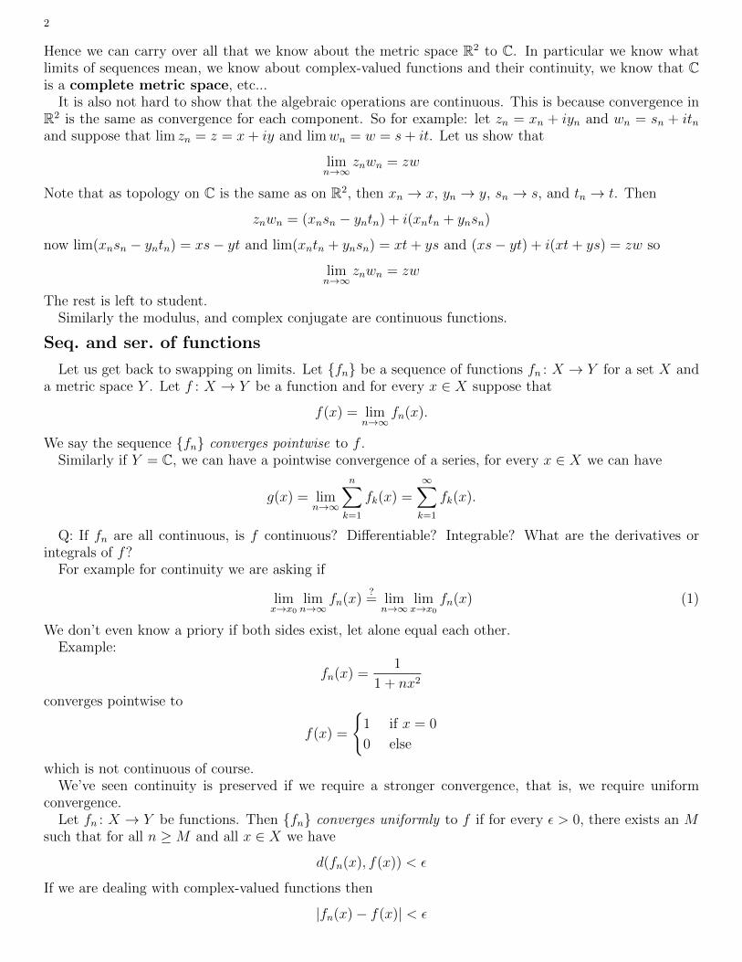
Hence we can carry over all that we know about the metric space R2 to C. In particular we know whatlimits of sequences mean, we know about complex-valued functions and their continuity, we know that Cis a complete metric space, etc...

It is also not hard to show that the algebraic operations are continuous. This is because convergence inR2 is the same as convergence for each component. So for example: let zn = xn + iyn and wn = sn + itnand suppose that lim zn = z = x+ iy and limwn = w = s+ it. Let us show that

limn→∞

znwn = zw

Note that as topology on C is the same as on R2, then xn → x, yn → y, sn → s, and tn → t. Then

znwn = (xnsn − yntn) + i(xntn + ynsn)

now lim(xnsn − yntn) = xs− yt and lim(xntn + ynsn) = xt+ ys and (xs− yt) + i(xt+ ys) = zw so

limn→∞

znwn = zw

The rest is left to student.Similarly the modulus, and complex conjugate are continuous functions.

Seq. and ser. of functions

Let us get back to swapping on limits. Let {fn} be a sequence of functions fn : X → Y for a set X anda metric space Y . Let f : X → Y be a function and for every x ∈ X suppose that

f(x) = limn→∞

fn(x).

We say the sequence {fn} converges pointwise to f .Similarly if Y = C, we can have a pointwise convergence of a series, for every x ∈ X we can have

g(x) = limn→∞

n∑k=1

fk(x) =∞∑k=1

fk(x).

Q: If fn are all continuous, is f continuous? Differentiable? Integrable? What are the derivatives orintegrals of f?

For example for continuity we are asking if

limx→x0

limn→∞

fn(x)?= lim

n→∞limx→x0

fn(x) (1)

We don’t even know a priory if both sides exist, let alone equal each other.Example:

fn(x) =1

1 + nx2

converges pointwise to

f(x) =

{1 if x = 0

0 else

which is not continuous of course.We’ve seen continuity is preserved if we require a stronger convergence, that is, we require uniform

convergence.Let fn : X → Y be functions. Then {fn} converges uniformly to f if for every ε > 0, there exists an M

such that for all n ≥M and all x ∈ X we have

d(fn(x), f(x)) < ε

If we are dealing with complex-valued functions then

|fn(x)− f(x)| < ε

3

Similarly a series of functions converges uniformly if the sequence of partial sums converges uniformly,that is for every ε > 0 ... we have ∣∣∣∣∣

(n∑k=1

fk(x)

)− f(x)

∣∣∣∣∣ < ε

Again recall from last semester that this is stronger than pointwise convergence. Pointwise convergencecan be stated as: {fn} converges pointwise to f if for every x ∈ X and every ε > 0, there exists an M suchthat for all n ≥M we have

d(fn(x), f(x)) < ε

Note that for uniform convergence M does not depend on x. We need to have one M that works for allM .

Theorem 7.8: Let fn : X → C be functions. Then {fn} converges uniformly if and only if for everyε > 0, there is an M such that for all n,m ≥M , and all x ∈ X we have

|fn(x)− fm(x)| < ε

Proof. Suppose that {fn} converges uniformly to some f : X → C. Then find M such that for all n ≥ Mwe have

|fn(x)− f(x)| < ε

2for all x ∈ X

Then for all m,n ≥M we have

|fn(x)− fm(x)| ≤ |fn(x)− f(x)|+ |f(x)− fm(x)| < ε

2+ε

2= ε

done.For the other direction, first fix x. The sequence of complex numbers {fn(x)} is Cauchy and so has a

limit f(x).Given ε > 0 find an M such that for all n,m ≥M , and all x ∈ X we have

|fn(x)− fm(x)| < ε

Now we know that lim fm(x) = f(x), so as compositions of continuous functions are continuous andalgebraic operations and the modulus are continuous we have

|fn(x)− f(x)| ≤ ε

(the nonstrict inequality is no trouble) �

Sometimes we write for f : X → C‖f‖u = sup

x∈X|f(x)| .

This is the supremum norm or uniform norm. Then we have that fn : X → C converge to f if and only if

limn→∞

‖fn − f‖u = 0

That is if

limn→∞

(supx∈X|fn(x)− f(x)|

)= 0

(That was Theorem 7.9)

If f : X → C is continuous and X is compact then ‖f‖u < ∞. With the metric d(f, g) = ‖f + g‖u theset of continuous complex-valued functions C(X,C) is a metric space (we have seen this for real-valuedfunctions which is almost the same). Let us check the triangle inequality.

|f(x) + g(x)| ≤ |f(x)|+ |g(x)| ≤ ‖f(x)‖u + ‖g(x)‖u .Now take a supremum on the left to get

‖f(x) + g(x)‖u ≤ ‖f(x)‖u + ‖g(x)‖u .

4

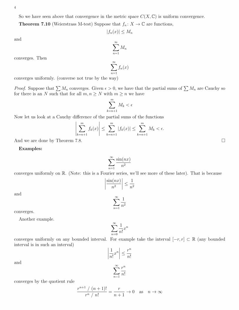
So we have seen above that convergence in the metric space C(X,C) is uniform convergence.

Theorem 7.10 (Weierstrass M-test) Suppose that fn : X → C are functions,

|fn(x)| ≤Mn

and∞∑n=1

Mn

converges. Then∞∑n=1

fn(x)

converges uniformly. (converse not true by the way)

Proof. Suppose that∑Mn converges. Given ε > 0, we have that the partial sums of

∑Mn are Cauchy so

for there is an N such that for all m,n ≥ N with m ≥ n we havem∑

k=n+1

Mk < ε

Now let us look at a Cauchy difference of the partial sums of the functions∣∣∣∣∣m∑

k=n+1

fk(x)

∣∣∣∣∣ ≤m∑

k=n+1

|fk(x)| ≤m∑

k=n+1

Mk < ε.

And we are done by Theorem 7.8. �

Examples:

∞∑n=1

sin(nx)

n2

converges uniformly on R. (Note: this is a Fourier series, we’ll see more of these later). That is because∣∣∣∣sin(nx)

n2

∣∣∣∣ ≤ 1

n2

and∞∑n=1

1

n2

converges.

Another example.∞∑n=0

1

n!xn

converges uniformly on any bounded interval. For example take the interval [−r, r] ⊂ R (any boundedinterval is in such an interval) ∣∣∣∣ 1

n!xn∣∣∣∣ ≤ rn

n!

and∞∑n=1

rn

n!

converges by the quotient rule

rn+1 / (n+ 1)!

rn / n!=

r

n+ 1→ 0 as n→∞

5

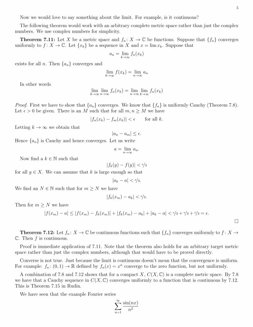
Now we would love to say something about the limit. For example, is it continuous?

The following theorem would work with an arbitrary complete metric space rather than just the complexnumbers. We use complex numbers for simplicity.

Theorem 7.11: Let X be a metric space and fn : X → C be functions. Suppose that {fn} convergesuniformly to f : X → C. Let {xk} be a sequence in X and x = limxk. Suppose that

an = limk→∞

fn(xk)

exists for all n. Then {an} converges and

limk→∞

f(xk) = limn→∞

an

In other words

limk→∞

limn→∞

fn(xk) = limn→∞

limk→∞

fn(xk)

Proof. First we have to show that {an} converges. We know that {fn} is uniformly Cauchy (Theorem 7.8).Let ε > 0 be given. There is an M such that for all m,n ≥M we have

|fn(xk)− fm(xk)| < ε for all k.

Letting k →∞ we obtain that

|an − am| ≤ ε.

Hence {an} is Cauchy and hence converges. Let us write

a = limn→∞

an.

Now find a k ∈ N such that

|fk(y)− f(y)| < ε/3

for all y ∈ X. We can assume that k is large enough so that

|ak − a| < ε/3.

We find an N ∈ N such that for m ≥ N we have

|fk(xm)− ak| < ε/3.

Then for m ≥ N we have

|f(xm)− a| ≤ |f(xm)− fk(xm)|+ |fk(xm)− ak|+ |ak − a| < ε/3 + ε/3 + ε/3 = ε.

�

Theorem 7.12: Let fn : X → C be continuous functions such that {fn} converges uniformly to f : X →C. Then f is continuous.

Proof is immediate application of 7.11. Note that the theorem also holds for an arbitrary target metricspace rather than just the complex numbers, although that would have to be proved directly.

Converse is not true. Just because the limit is continuous doesn’t mean that the convergence is uniform.For example: fn : (0, 1)→ R defined by fn(x) = xn converge to the zero function, but not uniformly.

A combination of 7.8 and 7.12 shows that for a compact X, C(X,C) is a complete metric space. By 7.8we have that a Cauchy sequence in C(X,C) converges uniformly to a function that is continuous by 7.12.This is Theorem 7.15 in Rudin.

We have seen that the example Fourier series∞∑n=1

sin(nx)

n2

6

converges uniformly and hence is continuous by 7.12. We note that this can be extended to show that ifthere is a constant C such that if α > 1

|an| ≤C

|n|α

for nonzero n ∈ Z, then the general Fourier series∞∑

n=−∞

aneinx

is a continuous function on R. (Note that eix = cos(x) + i sin(x) to write the series in terms of sines andcosines. The condition on those coefficients is the same). Also note that the standard way to sum a serieswith two infinite limits is

∞∑n=−∞

cn =

(limN→∞

N∑n=1

c−n

)+

(limN→∞

N∑n=0

cn

),

although for Fourier series we often sum it as

limN→∞

N∑n=−N

aneinx.

When the series converges absolutely it does not matter how we sum it.

Let us see that we can have extra conditions when a converse of 7.12 works.

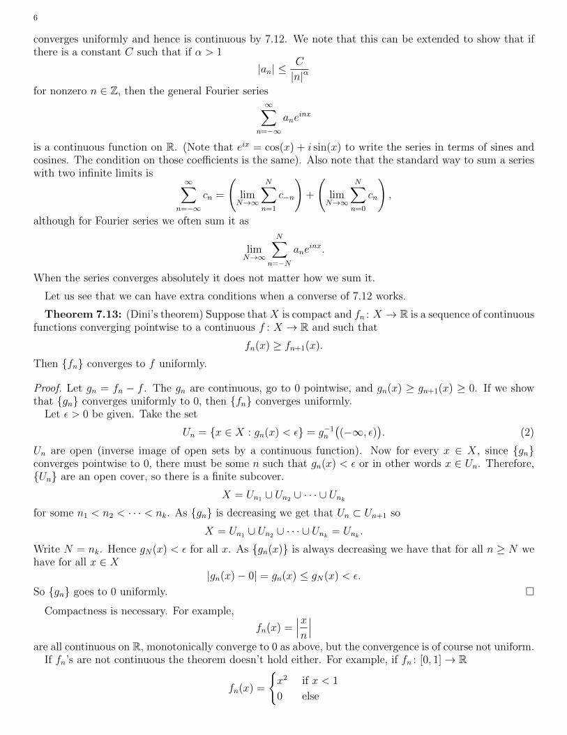
Theorem 7.13: (Dini’s theorem) Suppose that X is compact and fn : X → R is a sequence of continuousfunctions converging pointwise to a continuous f : X → R and such that

fn(x) ≥ fn+1(x).

Then {fn} converges to f uniformly.

Proof. Let gn = fn − f . The gn are continuous, go to 0 pointwise, and gn(x) ≥ gn+1(x) ≥ 0. If we showthat {gn} converges uniformly to 0, then {fn} converges uniformly.

Let ε > 0 be given. Take the set

Un = {x ∈ X : gn(x) < ε} = g−1n((−∞, ε)

). (2)

Un are open (inverse image of open sets by a continuous function). Now for every x ∈ X, since {gn}converges pointwise to 0, there must be some n such that gn(x) < ε or in other words x ∈ Un. Therefore,{Un} are an open cover, so there is a finite subcover.

X = Un1 ∪ Un2 ∪ · · · ∪ Unk

for some n1 < n2 < · · · < nk. As {gn} is decreasing we get that Un ⊂ Un+1 so

X = Un1 ∪ Un2 ∪ · · · ∪ Unk= Unk

.

Write N = nk. Hence gN(x) < ε for all x. As {gn(x)} is always decreasing we have that for all n ≥ N wehave for all x ∈ X

|gn(x)− 0| = gn(x) ≤ gN(x) < ε.

So {gn} goes to 0 uniformly. �

Compactness is necessary. For example,

fn(x) =∣∣∣xn

∣∣∣are all continuous on R, monotonically converge to 0 as above, but the convergence is of course not uniform.

If fn’s are not continuous the theorem doesn’t hold either. For example, if fn : [0, 1]→ R

fn(x) =

{x2 if x < 1

0 else

7

then {fn} goes monotonically pointwise to 0, and the domain is compact, but the convergence is notuniform (Exercise: see where the proof breaks).

Finally,

fn(x) =nx

1 + n2x2

are continuous, they go to zero pointwise (but not monotonically). If we take X = [0, 1] then the domainis compact, yet the convergence is not uniform since

fn(1/n) = 1/2 for all n.

Uniform convergence and integration.

Proposition: If fn : X → C are bounded functions and converge uniformly to f : X → C, then f isbounded.

Proof. There must exist an n such that

|fn(x)− f(x)| < 1

for all x. Now find M such that |fn(x)| ≤M for all x. By reverse triangle inequality

|f(x)| < 1 + |fn(x)| ≤ 1 +M.

�

We have seen Riemann integrals of real-valued functions. For complex-valued function f : [a, b]→ C, wewrite f(x) = u(x) + iv(x) where u and v are real-valued. We say f is Riemann integrable if both u and vare, in which case ∫ b

a

f =

∫ b

a

u+ i

∫ b

a

v

So most statements about real-valued Riemann integrable functions just carry over immediately to complex-valued functions.

We will not do Riemann-Stieltjes integration like Rudin, just Riemann.

Theorem 7.16: Suppose that fn : [a, b]→ C are Riemann integrable and suppose that {fn} convergesuniformly to f : [a, b]→ C. Then f is Riemann integrable and∫ b

a

f = limn→∞

∫ b

a

fn

Proof. Without loss of generality suppose that fn, and hence f , are all real-valued. As fn are all bounded,we have that f is bounded by above proposition.

Let ε > 0 be given. As fn goes to f uniformly, we find an M ∈ N such that for all n ≥ M we have|fn(x)− f(x)| < ε

2(b−a) for all x ∈ [a, b]. Note that fn is integrable and compute∫ b

a

f −∫ b

a

f =

∫ b

a

(f(x)− fn(x) + fn(x)

)dx−

∫ b

a

(f(x)− fn(x) + fn(x)

)dx

=

∫ b

a

(f(x)− fn(x)

)dx+

∫ b

a

fn(x) dx−∫ b

a

(f(x)− fn(x)

)dx−

∫ b

a

fn(x) dx

=

∫ b

a

(f(x)− fn(x)

)dx+

∫ b

a

fn(x) dx−∫ b

a

(f(x)− fn(x)

)dx−

∫ b

a

fn(x) dx

=

∫ b

a

(f(x)− fn(x)

)dx−

∫ b

a

(f(x)− fn(x)

)dx

≤ ε

2(b− a)(b− a) +

ε

2(b− a)(b− a) = ε.

8

The inequality follows from the fact that for all x ∈ [a, b] we have −ε2(b−a) < f(x)− fn(x) < ε

2(b−a) . As ε > 0

was arbitrary, f is Riemann integrable.

Finally we compute∫ baf . Again, for n ≥M (where M is the same as above) we have∣∣∣∣∫ b

a

f −∫ b

a

fn

∣∣∣∣ =

∣∣∣∣∫ b

a

(f(x)− fn(x)

)dx

∣∣∣∣≤ ε

2(b− a)(b− a) =

ε

2< ε.

Therefore {∫ bafn} converges to

∫ baf . �

Corollary: Suppose that fn : [a, b]→ C are Riemann integrable and suppose that

∞∑n=1

fn(x)

converges uniformly. Then the series is Riemann integrable on [a, b] and∫ b

a

∞∑n=1

fn(x) dx =∞∑n=1

∫ b

a

fn(x) dx

Example: Let us show how to integrate a Fourier series. used for convenience.∫ x

0

∞∑n=1

cos(nt)

n2dt =

∞∑n=1

∫ x

0

cos(nt)

n2dt =

∞∑n=1

sin(nx)

n3

The swapping of integral and sum is possible because of uniform convergence, which we have proved beforeusing the M test.

Note that we can swap integrals and limits under far less stringent hypotheses, but for that we wouldneed a stronger integral than Riemann integral. E.g. the Lebesgue integral.

Differentiation

Example: Let fn(x) = 11+nx2

. We know this converges pointwise to a function that is zero except atthe origin. Now note that

f ′n(x) =−2nx

(1 + nx2)2

No matter what x is limn→∞ f′n(x) = 0. So the derivatives converge pointwise to 0 (not uniformly on any

closed interval containing 0), while the limit of fn is not even differentiable at 0 (not even continuous).

Example: Let fn(x) = sin(n2x)n

, then fn → 0 uniformly on R (easy). However

f ′n(x) = n cos(n2x)

And for example at x = 0, this doesn’t even converge. So we need something stronger than uniformconvergence of fn.

For complex-valued functions, again, the derivative of f : [a, b]→ C where f(x) = u(x) + iv(x) is

f ′(x) = u′(x) + iv′(x).

Theorem 7.17: Suppose fn : [a, b]→ C are differentiable on [a, b]. Suppose that there is some point x0 ∈[a, b] such that {fn(x0)} converges, and such that {f ′n} converge uniformly. Then there is a differentiablefunction f such that {fn} converges uniformly to f , and furthermore

f ′(x) = limn→∞

f ′n(x) for all x ∈ [a, b].

9

Proof. Let ε > 0 be given. We have that {fn(x0)} is Cauchy so there is an N such that for n,m ≥ N wehave

|fn(x0)− fm(x0)| < ε/2

We also that that {f ′n} converge uniformly and hence is uniformly Cauchy, so also assume that for all xwe have

|f ′n(x)− f ′m(x)| < ε

2(b− a)

Now we have the mean value theorem (for complex-valued function just apply the theorem on both realand imaginary parts separately) for the differentiable function fn − fm, so for x0, x in [a, b] there is a tbetween x0 and x such that

(fn(x0)− fm(x0))− (fn(x)− fm(x)) = (f ′n(t)− f ′m(t))(x0 − x)

and so

|(fn(x0)− fm(x0))− (fn(x)− fm(x))| = |f ′n(t)− f ′m(t)| |x0 − x| <ε

2(b− a)|x0 − x| ≤

ε

2

and so by inverse triangle inequality

|fn(x)− fm(x)| ≤ |(fn(x0)− fm(x0))− (fn(x)− fm(x))|+ |fn(x0)− fm(x0)| <ε

2+ε

2= ε.

This was true for all x ∈ [a, b] so {fn} is uniformly Cauchy and so the sequence converges uniformly tosome f : [a, b]→ C.

So what we are still missing is that f is differentiable and that its derivative is the right thing.Call g : [a, b]→ C the limit of {f ′n}. Fix x ∈ [a, b] and take the functions

ϕn(t) =

{fn(x)−fn(t)

x−t if t 6= x,

f ′n(x) if t = x,

ϕ(t) =

{f(x)−f(t)

x−t if t 6= x,

g(x) if t = x.

The functions ϕn(t) are continuous (in particular continuous at x). Given an ε > 0 we get that there issome N such that for m,n ≥ N we have that |f ′n(y)− f ′m(y)| < ε for all y ∈ [a, b]. Then by the same logicas above using the mean value theorem we get for all t

|(fn(x)− fn(t))− (fm(x)− fm(t))| = |(fn(x)− fm(x))− (fn(t)− fm(t))| < ε |x− t|Or in other words

|ϕn(t)− ϕm(t)| < ε for all t.

So {ϕn} converges uniformly. The limit is therefore a continuous function. It is easy to see that for a fixedt 6= x, limϕn(t) = ϕ(t) and since g is the limit of {f ′n} also limϕn(x) = ϕ(x). Therefore, ϕ is the limit andis therefore continuous. This means that f is differentiable at x and that f ′(x) = g(x). As x was arbitrarywe are done. �

Note that continuity of f ′n would make the proof far easier and could be done by fundamental theorem ofcalculus, and the passing of limit under the integral. The trick above is that we have no such assumption.

Example: Let us see what this means for Fourier series∞∑

n=−∞

aneinx

and suppose that for some C and some α > 2 that for all nonzero n ∈ Z we have

|an| ≤C

|n|α.

Not only does the series converge, but it is also continuously differentiable, and the derivative is obtainedby differentiation termwise.

10

The trick to this is that 1) At x = 0 we converge (duh!). 2) If we differentiate the partial sums theresulting partial sums converge absolutely as we are looking at sums such as

M∑n=m

inaneinx

where we are letting m go to −∞ and M go to ∞. So for the coefficients we have

|inan| ≤C

|n|α−1

and the differentiated series will converge uniformly by the M-test.

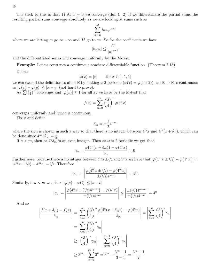
Example: Let us construct a continuous nowhere differentiable function. (Theorem 7.18)

Defineϕ(x) = |x| for x ∈ [−1, 1]

we can extend the definition to all of R by making ϕ 2-periodic (ϕ(x) = ϕ(x+2)). ϕ : R→ R is continuousas |ϕ(x)− ϕ(y)| ≤ |x− y| (not hard to prove).

As∑(

34

)nconverges and |ϕ(x)| ≤ 1 for all x, we have by the M-test that

f(x) =∞∑n=0

(3

4

)nϕ(4nx)

converges uniformly and hence is continuous.Fix x and define

δm = ±1

24−m

where the sign is chosen in such a way so that there is no integer between 4mx and 4m(x+ δm), which canbe done since 4m |δm| = 1

2.

If n > m, then as 4nδm is an even integer. Then as ϕ is 2-periodic we get that

γn =ϕ(4n(x+ δm)

)− ϕ(4nx)

δm= 0

Furthermore, because there is no integer between 4mx±1/2 and 4mx we have that |ϕ(4mx± 1/2)− ϕ(4mx)| =|4mx± 1/2)− 4mx| = 1/2. Therefore

|γm| =∣∣∣∣ϕ(4mx± 1/2)− ϕ(4mx)

±(1/2)4−m

∣∣∣∣ = 4m.

Similarly, if n < m we, since |ϕ(s)− ϕ(t)| ≤ |s− t|

|γn| =

∣∣∣∣∣ϕ(4nx± (1/2)4n−m

)− ϕ(4nx)

±(1/2)4−m

∣∣∣∣∣ ≤∣∣∣∣±(1/2)4n−m

±(1/2)4−m

∣∣∣∣ = 4n

And so ∣∣∣∣f(x+ δm)− f(x)

δm

∣∣∣∣ =

∣∣∣∣∣∞∑n=0

(3

4

)nϕ(4n(x+ δm))− ϕ(4nx)

δm

∣∣∣∣∣ =

∣∣∣∣∣∞∑n=0

(3

4

)nγn

∣∣∣∣∣=

∣∣∣∣∣m∑n=0

(3

4

)nγn

∣∣∣∣∣≥∣∣∣∣(3

4

)mγm

∣∣∣∣−∣∣∣∣∣m−1∑n=0

(3

4

)nγn

∣∣∣∣∣≥ 3m −

m−1∑n=0

3n = 3m − 3m − 1

3− 1=

3m + 1

2

11

It is obvious that δm → 0 as m→∞, but 3m+12

goes to infinity. Hence f cannot be differentiable at x.We will see later that such an f is a uniform limit of not just differentiable functions but actually it is

the uniform limit of polynomials.

Equicontinuity

We would like an analogue of Bolzano-Weierstrass, that is every bounded sequence of functions has aconvergent subsequence. Matters will not be as simple of course even for continuous functions. Recallfrom last semester that not every bounded set in the metric space C(X,R) was compact, so a boundedsequence in the metric space C(X,R) may not have a convergent subsequence.

Definition: Let fn : X → C be a sequence. We say that {fn} is pointwise bounded if for every x ∈ X,there is an Mx ∈ R such that

|fn(x)| ≤Mx for all n ∈ NWe say that {fn} is uniformly bounded if there is an M ∈ R such that

|fn(x)| ≤M for all n ∈ N and all x ∈ X

Note that uniform boundedness is the same as boundedness in the metric space C(X,C) (assuming thatX is compact)

We don’t have the machinery yet to easily exhibit a sequence of continuous functions on [0, 1] thatis uniformly bounded but contains no subsequence converging even pointwise. Let us just state thatfn(x) = sin(2πnx) is one such sequence.

We also of course have that fn(x) = xn is a sequence that is uniformly bounded, but contains no sequencethat converges uniformly (it does converge pointwise though).

When the domain is countable, matters are easier. We will also use the following theorem as a lemmalater. It will use a very common and useful diagonal argument.

Theorem 7.23: Let X be countable and fn : X → C give a pointwise bounded sequence of functions,then {fn} has a subsequence that converges pointwise.

Proof. Let {xk} be an enumeration of the elements of X. The sequence {fn(x1)}∞n=1 is bounded and hencewe have a subsequence which we will denote by f1,k such that {f1,k(x1)} converges. Next {f1,k(x2)} hasa subsequence that converges and we denote that subsequence by {f2,k(x2)}. In general we will have asequence {fm,k}k that makes {fm,k(xj)}k converge for all j ≤ m and we will let {fm+1,k}k be the subsequenceof {fm,k}k such that {fm+1,k(xm+1)}k converges (and hence it converges for all xj for j = 1, . . . ,m+ 1) andwe can rinse and repeat.

Finally pick the sequence {fk,k}. This is a subsequence of the original sequence {fn} of course. Also forany m, except for the first m terms {fk, k} is a subsequence of {fm,k}k and hence for any m the sequence{fk,k(xm)}k converges. �

For larger than countable sets, we need the functions of the sequence to be related. We look at continuousfunctions, and the concept we need is equicontinuity.

Definition: a family F of functions f : X → C is said to be equicontinuous on X if for every ε > 0, thereis a δ > 0 such that if x, y ∈ X with d(x, y) < δ we have

|f(x)− f(y)| < ε for all f ∈ F .One obvious fact is that if F is equicontinuous, then every element of f is uniformly continuous. Also

obvious is that any finite set of uniformly continuous functions is an equicontinuous family. Of coursethe interesting case is when F is an infinite family such as a sequence of functions. Equicontinuity of asequence is closely related to uniform convergence.

First a proposition, that we have proved for compact intervals before.

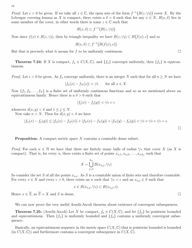
Proposition: If X is compact and f : X → C is continuous, then f is uniformly continuous.

12

Proof. Let ε > 0 be given. If we take all z ∈ C, the open sets of the form f−1(B(z, ε/2)

)cover X. By the

Lebesgue covering lemma as X is compact, there exists a δ > 0 such that for any x ∈ X, B(x, δ) lies insome member of the cover, in other words there is some z ∈ C such that

B(x, δ) ⊂ f−1(B(z, ε/2)

)Now since f(x) ∈ B(z, ε/2), then by triangle inequality we have B(z, ε/2) ⊂ B

(f(x), ε

)and so

B(x, δ) ⊂ f−1(B(f(x), ε)

)But that is precisely what it means for f to be uniformly continuous. �

Theorem 7.24: If X is compact, fn ∈ C(X,C), and {fn} converges uniformly, then {fn} is equicon-tinuous.

Proof. Let ε > 0 be given. As fn converge uniformly, there is an integer N such that for all n ≥ N we have

|fn(x)− fN(x)| < ε/3 for all x ∈ X.

Now {f1, f2, . . . , fN} is a finite set of uniformly continuous functions and so as we mentioned above anequicontinuous family. Hence there is a δ > 0 such that

|fj(x)− fj(y)| < ε/3 < ε

whenever d(x, y) < δ and 1 ≤ j ≤ N .Now take n > N . Then for d(x, y) < δ we have

|fn(x)− fn(y)| ≤ |fn(x)− fN(x)|+ |fN(x)− fN(y)|+ |fN(y)− fn(y)| < ε/3 + ε/3 + ε/3 = ε.

�

Proposition: A compact metric space X contains a countable dense subset.

Proof. For each n ∈ N we have that there are finitely many balls of radius 1/n that cover X (as X iscompact). That is, for every n, there exists a finite set of points xn,1, xn,2, . . . , xn,kn such that

X =kn⋃j=1

B(xn,j, 1/n)

So consider the set S of all the points xn,j. As S is a countable union of finite sets and therefore countable.For every x ∈ X and every ε > 0, there exists an n such that 1/n < ε and an xn,j ∈ S such that

x ∈ B(xn,j, 1/n) ⊂ B(xn,j, ε).

Hence x ∈ S, so S = X and S is dense. �

We can now prove the very useful Arzela-Ascoli theorem about existence of convergent subsequences.

Theorem 7.25: (Arzela-Ascoli) Let X be compact, fn ∈ C(X,C), and let {fn} be pointwise boundedand equicontinuous. Then {fn} is uniformly bounded and {fn} contains a uniformly convergent subse-quence.

Basically, an equicontinuous sequence in the metric space C(X,C) that is pointwise bounded is bounded(in C(X,C)) and furthermore contains a convergent subsequence in C(X,C).

13

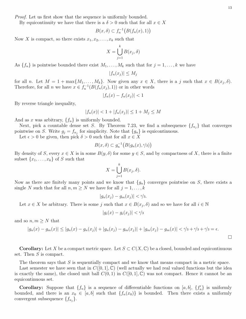
Proof. Let us first show that the sequence is uniformly bounded.By equicontinuity we have that there is a δ > 0 such that for all x ∈ X

B(x, δ) ⊂ f−1n(B(fn(x), 1)

)Now X is compact, so there exists x1, x2, . . . , xk such that

X =k⋃j=1

B(xj, δ)

As {fn} is pointwise bounded there exist M1, . . . ,Mk such that for j = 1, . . . , k we have

|fn(xj)| ≤Mj

for all n. Let M = 1 + max{M1, . . . ,Mk}. Now given any x ∈ X, there is a j such that x ∈ B(xj, δ).Therefore, for all n we have x ∈ f−1n (B(fn(xj), 1)) or in other words

|fn(x)− fn(xj)| < 1

By reverse triangle inequality,

|fn(x)| < 1 + |fn(xj)| ≤ 1 +Mj ≤M

And as x was arbitrary, {fn} is uniformly bounded.Next, pick a countable dense set S. By Theorem 7.23, we find a subsequence {fnj

} that convergespointwise on S. Write gj = fnj

for simplicity. Note that {gn} is equicontinuous.Let ε > 0 be given, then pick δ > 0 such that for all x ∈ X

B(x, δ) ⊂ g−1n(B(gn(x), ε/3)

)By density of S, every x ∈ X is in some B(y, δ) for some y ∈ S, and by compactness of X, there is a finitesubset {x1, . . . , xk} of S such that

X =k⋃j=1

B(xj, δ).

Now as there are finitely many points and we know that {gn} converges pointwise on S, there exists asingle N such that for all n,m ≥ N we have for all j = 1, . . . , k

|gn(xj)− gm(xj)| < ε/3.

Let x ∈ X be arbitrary. There is some j such that x ∈ B(xj, δ) and so we have for all i ∈ N

|gi(x)− gi(xj)| < ε/3

and so n,m ≥ N that

|gn(x)− gm(x)| ≤ |gn(x)− gn(xj)|+ |gn(xj)− gm(xj)|+ |gm(xj)− gm(x)| < ε/3 + ε/3 + ε/3 = ε.

�

Corollary: LetX be a compact metric space. Let S ⊂ C(X,C) be a closed, bounded and equicontinuousset. Then S is compact.

The theorem says that S is sequentially compact and we know that means compact in a metric space.Last semester we have seen that in C([0, 1],C) (well actually we had real valued functions but the idea

is exactly the same), the closed unit ball C(0, 1) in C([0, 1],C) was not compact. Hence it cannot be anequicontinuous set.

Corollary: Suppose that {fn} is a sequence of differentiable functions on [a, b], {f ′n} is uniformlybounded, and there is an x0 ∈ [a, b] such that {fn(x0)} is bounded. Then there exists a uniformlyconvergent subsequence {fnj

}.

14

Proof. The trick is to use the mean value theorem. If M is the uniform bound on {f ′n}, then we have bythe mean value theorem

|fn(x)− fn(y)| ≤M |x− y|So all the fn’s are Lipschitz with the same constant and hence equicontinuous.

Now suppose that |fn(x0)| ≤M0 for all n. By inverse triangle inequality we have for all x

|fn(x)| ≤ |fn(x0)|+ |fn(x)− fn(x0)| ≤M0 +M |x− x0| ≤M0 +M(b− a)

so {fn} is uniformly bounded.We can now apply Arzela-Ascoli to find the subsequence. �

A consequence of the above corollary and the Fundamental Theorem of Calculus is that given some fixedg ∈ C([0, 1],C), the set of functions

{F ∈ C([0, 1],C) : F (x) =

∫ x

0

g(t)f(t) dt, f ∈ C([0, 1],C), ‖f‖u ≤ 1}

has compact closure (relatively compact). That is, the operator T : C([0, 1],C)→ C([0, 1],C) given by

T(f)(x) = F (x) =

∫ x

0

g(t)f(t) dt

takes the unit ball centered at 0 in C([0, 1],C) into a relatively compact set. We often say that this meansthat the operator is compact, and such operators are very important (and very useful).

Stone-Weierstrass

Perhaps surprisingly, even a very badly behaving continuous function is really just a uniform limit ofpolynomials. We cannot really get any “nicer” as a function than a polynomial.

Theorem 7.26 (Weierstrass approximation theorem) If f : [a, b]→ C is continuous, then there exists asequence {pn} of polynomials converging to f uniformly on [a, b]. Furthermore, if f is real-valued, we canfind real-valued pn.

Proof. For x ∈ [0, 1] define

g(x) = f((b− a)x+ a

)− f(a)− x

(f(b)− f(a)

).

If we can prove the theorem for g and find the {pn} for g, we can prove it for f since we simply composedwith an invertible affine function and added an affine function to f , so we can easily reverse the processand apply that to our pn, to obtain polynomials approximating f .

So g is defined on [0, 1] and g(0) = g(1) = 0. We can now assume that g is defined on the whole realline for simplicity by defining g(x) = 0 if x < 0 or x > 1.

Let

cn =

(∫ 1

−1(1− x2)n dx

)−1Then define

qn(x) = cn(1− x2)n

so that∫ 1

−1 qn(x) dx = 1.We note that qn are peaks around 0 (ignoring what happens outside of [−1, 1]) that get narrower and

narrower. You should plot a few of these to see what is happening. A classic approximation idea is to doa convolution integral with peaks like this. That is we will write for x ∈ [0, 1],

pn(x) =

∫ 1

0

g(t)qn(t− x) dt

(=

∫ ∞−∞

g(t)qn(t− x) dt

).

Because qn is a polynomial we can write

qn(t− x) = a0(t) + a1(t)x+ · · ·+ a2n(t)x2n

15

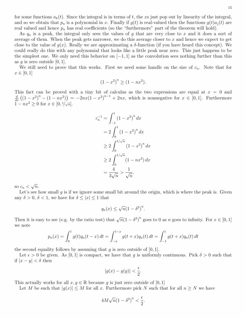
for some functions ak(t). Since the integral is in terms of t, the xs just pop out by linearity of the integral,and so we obtain that pn is a polynomial in x. Finally if g(t) is real-valued then the functions g(t)aj(t) arereal valued and hence pn has real coefficients (so the “furthermore” part of the theorem will hold).

As qn is a peak, the integral only sees the values of g that are very close to x and it does a sort ofaverage of them. When the peak gets narrower, we do this average closer to x and hence we expect to getclose to the value of g(x). Really we are approximating a δ-function (if you have heard this concept). Wecould really do this with any polynomial that looks like a little peak near zero. This just happens to bethe simplest one. We only need this behavior on [−1, 1] as the convolution sees nothing further than thisas g is zero outside [0, 1].

We still need to prove that this works. First we need some handle on the size of cn. Note that forx ∈ [0, 1]

(1− x2)n ≥ (1− nx2).

This fact can be proved with a tiny bit of calculus as the two expressions are equal at x = 0 andddx

((1− x2)n − (1− nx2)

)= −2nx(1− x2)n−1 + 2nx, which is nonnegative for x ∈ [0, 1]. Furthermore

1− nx2 ≥ 0 for x ∈ [0, 1/√n].

c−1n =

∫ 1

−1(1− x2)n dx

= 2

∫ 1

0

(1− x2)n dx

≥ 2

∫ 1/√n

0

(1− x2)n dx

≥ 2

∫ 1/√n

0

(1− nx2) dx

=4

3√n>

1√n.

so cn <√n.

Let’s see how small g is if we ignore some small bit around the origin, which is where the peak is. Givenany δ > 0, δ < 1, we have for δ ≤ |x| ≤ 1 that

qn(x) ≤√n(1− δ2)n.

Then it is easy to see (e.g. by the ratio test) that√n(1− δ2)n goes to 0 as n goes to infinity. For x ∈ [0, 1]

we note

pn(x) =

∫ 1

0

g(t)qn(t− x) dt =

∫ 1−x

−xg(t+ x)qn(t) dt =

∫ 1

−1g(t+ x)qn(t) dt

the second equality follows by assuming that g is zero outside of [0, 1].Let ε > 0 be given. As [0, 1] is compact, we have that g is uniformly continuous. Pick δ > 0 such that

if |x− y| < δ then

|g(x)− g(y)| < ε

2.

This actually works for all x, y ∈ R because g is just zero outside of [0, 1]Let M be such that |g(x)| ≤M for all x. Furthermore pick N such that for all n ≥ N we have

4M√n(1− δ2)n < ε

2.

16

Note that∫ 1

−1 qn(t) dt = 1 and qn(x) ≥ 0 on [−1, 1] so

|pn(x)− g(x)| =∣∣∣∣∫ 1

−1g(t+ x)qn(t) dt− g(x)

∫ 1

−1qn(t) dt

∣∣∣∣=

∣∣∣∣∫ 1

−1

(g(t+ x)− g(x)

)qn(t) dt

∣∣∣∣≤∫ 1

−1|g(t+ x)− g(x)| qn(t) dt

=

∫ −δ−1|g(t+ x)− g(x)| qn(t) dt+

∫ δ

−δ|g(t+ x)− g(x)| qn(t) dt+

∫ 1

δ

|g(t+ x)− g(x)| qn(t) dt

≤ 2M

∫ −δ−1

qn(t) dt+ε

2

∫ δ

−δqn(t) dt+ 2M

∫ 1

δ

qn(t) dt

≤ 2M√n(1− δ2)n(1− δ) +

ε

2+ 2M

√n(1− δ2)n(1− δ)

< 4M√n(1− δ2)n +

ε

2< ε.

�

Think about the consequences of the theorem. If you have any property that gets preserved underuniform convergence and it is true for polynomials, then it must be true for all continuous functions.

Let us note an immediate application of the Weierstrass theorem. We have already seen that countabledense subsets can be very useful.

Corollary: The metric space C([a, b],C) contains a countable dense subset.

Proof. Without loss of generality suppose that we are dealing with C([a, b],R) (why can we?). The realpolynomials are dense in C([a, b],R). If we can show that any real polynomial can be approximated bypolynomials with rational coefficients, we are done. This is because there are only countably many rationalnumbers and so there are only countably many polynomials with rational coefficients (a countable unionof countable sets is still countable).

Further without loss of generality, suppose that [a, b] = [0, 1]. Let

p(x) =n∑k=0

akxk

be a polynomial of degree n where ak ∈ R. Given ε > 0, pick bk ∈ Q such that |ak − bk| < εn+1

. Then ifwe let

q(x) =n∑k=0

bkxk

we have

|p(x)− q(x)| =

∣∣∣∣∣n∑k=0

(ak − bk)xk∣∣∣∣∣ ≤

n∑k=0

|ak − bk|xk ≤n∑k=0

|ak − bk| <n∑k=0

ε

n+ 1= ε

�

Funky remark: While we will not prove this, we note that the above corollary implies that C([a, b],C)has the same cardinality as the real numbers, which may be a bit surprising. The set of all functions[a, b] → C has cardinality that is strictly greater than the cardinality of R, it has the cardinality of thepower set of R. So the set of continuous functions is a very tiny subset of the set of all functions.

Next thing we do is that we will want to abstract away what is not really necessary and prove a generalversion of this theorem. We have shown that the polynomials are dense in the space of continuous functions

17

on a compact interval. So what kind of families of functions are also dense? Furthermore, what if we letthe domain be an arbitrary metric space, then we no longer have polynomials.

The resulting theorem is the Stone-Weierstrass theorem. We will need a special case of the Weierstrasstheorem though.

Corollary: Let [−a, a] be an interval. Then there is a sequence of real polynomials {pn} that convergesuniformly to |x| on [−a, a] and such that pn(0) = 0 for all n.

Proof. As f(x) = |x| is continuous and real-valued on [−a, a] we definitely have some real polynomials pnthat converge to f . Let

pn(x) = pn(x)− pn(0)

Obviously pn(0) = 0.We know lim pn(0) = 0. Given ε > 0, let N be such that for n ≥ N we have |pn(0)| < ε/2 and also that∣∣pn(x)− |x|

∣∣ < ε/2. Now∣∣pn(x)− |x|∣∣ =

∣∣pn(x)− pn(0)− |x|∣∣ ≤ ∣∣pn(x)− |x|

∣∣+ |pn(0)| < ε/2 + ε/2 = ε.

�

Following the proof of the theorem, we see that we can always make the polynomials from the Weierstrasstheorem have a fixed value at one point, so it works not just for |x|.

Definition: A family A of complex-valued functions f : X → C is said to be an algebra (sometimescomplex algebra or algebra over C) if for all f, g ∈ A and c ∈ C we have

(i) f + g ∈ A,(ii) fg ∈ A, and(iii) cg ∈ A.

If we talk of an algebra of real-valued functions (sometimes real algebra or algebra over R), then ofcourse we only need the above to hold for c ∈ R.

We say that A is uniformly closed if the limit of every uniformly convergent sequence in A is also in A.Similarly, a set B of all uniform limits of uniformly convergent sequences in A is said to be the uniformclosure of A.

If X is a compact metric space and A is a subset of the metric space C(X,C), then the uniform closureof A is just the metric space closure A in C(X,C), of course.

For example, the set P of all polynomials is an algebra in C(X,C), and we have shown that its uniformclosure is all of C(X,C).

Theorem 7.29: Let A be an algebra of bounded functions on a set X, and let B be its uniform closure.Then B is a uniformly closed algebra.

Proof. Let f, g ∈ B and c ∈ C. Then there are uniformly convergent sequences of functions {fn}, {gn} inA such that f is the uniform limit of {fn} and g is the uniform limit of {gn}.

What we want is to show that fn + gn converges uniformly to f + g, fngn converges uniformly to fg,and cfn converges uniformly to cf . As f and g are bounded, then we have seen that {fn} and {gn} arealso uniformly bounded. Therefore there is a single number M such that for all x ∈ X we have

|fn(x)| ≤M, |gn(x)| ≤M, |f(x)| ≤M, |g(x)| ≤M.

The following estimates are enough to show uniform convergence.∣∣(fn(x) + gn(x))−(f(x) + g(x)

)∣∣ ≤ |fn(x)− f(x)|+ |gn(x)− g(x)|

|fn(x)gn(x)− f(x)g(x)| ≤ |fn(x)gn(x)− fn(x)g(x)|+ |fn(x)g(x)− f(x)g(x)|≤M |gn(x)− g(x)|+M |fn(x)− f(x)|

|cfn(x)− cf(x)| = |c| |fn(x)− f(x)|

18

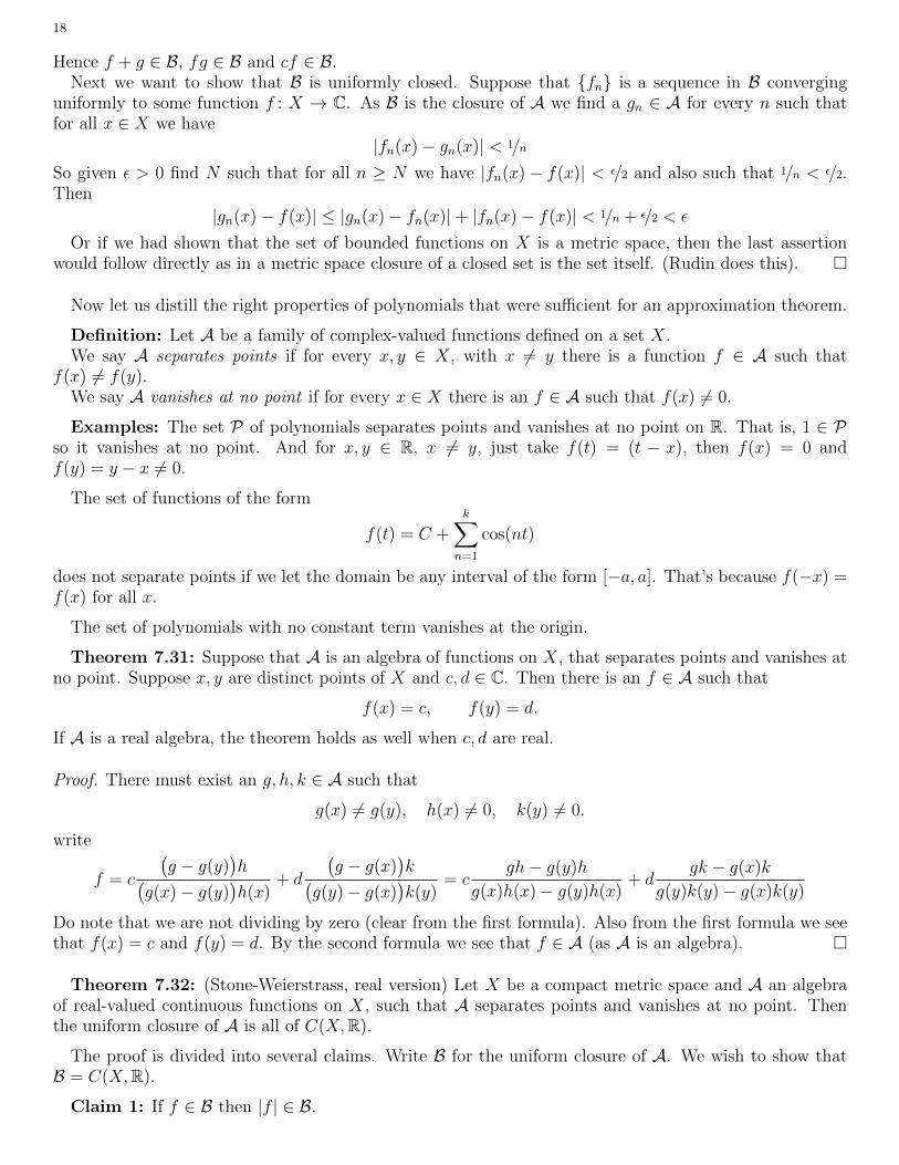
Hence f + g ∈ B, fg ∈ B and cf ∈ B.Next we want to show that B is uniformly closed. Suppose that {fn} is a sequence in B converging

uniformly to some function f : X → C. As B is the closure of A we find a gn ∈ A for every n such thatfor all x ∈ X we have

|fn(x)− gn(x)| < 1/n

So given ε > 0 find N such that for all n ≥ N we have |fn(x)− f(x)| < ε/2 and also such that 1/n < ε/2.Then

|gn(x)− f(x)| ≤ |gn(x)− fn(x)|+ |fn(x)− f(x)| < 1/n + ε/2 < ε

Or if we had shown that the set of bounded functions on X is a metric space, then the last assertionwould follow directly as in a metric space closure of a closed set is the set itself. (Rudin does this). �

Now let us distill the right properties of polynomials that were sufficient for an approximation theorem.

Definition: Let A be a family of complex-valued functions defined on a set X.We say A separates points if for every x, y ∈ X, with x 6= y there is a function f ∈ A such that

f(x) 6= f(y).We say A vanishes at no point if for every x ∈ X there is an f ∈ A such that f(x) 6= 0.

Examples: The set P of polynomials separates points and vanishes at no point on R. That is, 1 ∈ Pso it vanishes at no point. And for x, y ∈ R, x 6= y, just take f(t) = (t − x), then f(x) = 0 andf(y) = y − x 6= 0.

The set of functions of the form

f(t) = C +k∑

n=1

cos(nt)

does not separate points if we let the domain be any interval of the form [−a, a]. That’s because f(−x) =f(x) for all x.

The set of polynomials with no constant term vanishes at the origin.

Theorem 7.31: Suppose that A is an algebra of functions on X, that separates points and vanishes atno point. Suppose x, y are distinct points of X and c, d ∈ C. Then there is an f ∈ A such that

f(x) = c, f(y) = d.

If A is a real algebra, the theorem holds as well when c, d are real.

Proof. There must exist an g, h, k ∈ A such that

g(x) 6= g(y), h(x) 6= 0, k(y) 6= 0.

write

f = c

(g − g(y)

)h(

g(x)− g(y))h(x)

+ d

(g − g(x)

)k(

g(y)− g(x))k(y)

= cgh− g(y)h

g(x)h(x)− g(y)h(x)+ d

gk − g(x)k

g(y)k(y)− g(x)k(y)

Do note that we are not dividing by zero (clear from the first formula). Also from the first formula we seethat f(x) = c and f(y) = d. By the second formula we see that f ∈ A (as A is an algebra). �

Theorem 7.32: (Stone-Weierstrass, real version) Let X be a compact metric space and A an algebraof real-valued continuous functions on X, such that A separates points and vanishes at no point. Thenthe uniform closure of A is all of C(X,R).

The proof is divided into several claims. Write B for the uniform closure of A. We wish to show thatB = C(X,R).

Claim 1: If f ∈ B then |f | ∈ B.

19

Proof. f is bounded (continuous on a compact set) for example |f(x)| ≤M for all x ∈ X.Let ε > 0 be given. By the corollary to Weierstrass theorem there exists a real polynomial c1y + c2y

2 +· · ·+ cny

n (vanishing at y = 0) such that ∣∣∣∣∣|y| −N∑j=1

cjyj

∣∣∣∣∣ < ε

for all y ∈ [−M,M ]. Because A is an algebra (note there is no constant term in the polynomial) we havethat

g =N∑j=1

cjfj ∈ A.

As |f(x)| ≤M we have that ∣∣|f(x)| − g(x)∣∣ =

∣∣∣∣∣|f(x)| −N∑j=1

cj(f(x))j

∣∣∣∣∣ < ε.

So |f | is in the closure of B, which is closed, so |f | ∈ B. �

Claim 2: If f ∈ B and g ∈ B then max(f, g) ∈ B and min(f, g) ∈ B, where(max(f, g)

)(x) = max{f(x), g(x)}

(min(f, g)

)(x) = min{f(x), g(x)}

Proof. Write:

max(f, g) =f + g

2+|f − g|

2,

and

min(f, g) =f + g

2− |f − g|

2.

As B is an algebra we are done. �

The claim is of course true for the minimum or maximum of any finite collection of functions as well.

Claim 3: Given f ∈ C(X,R), x ∈ X and ε > 0 there exists a gx ∈ B with gx(x) = f(x) and

gx(t) > f(t)− ε for all t ∈ X.

Proof. Let x ∈ X be fixed. By Theorem 7.31, for every y ∈ X we find an hy ∈ A such that

hy(x) = f(x), hy(y) = f(y)

As hy and f are continuous, the set

Jy = {t ∈ X : hy(t) > f(t)− ε}is open (it is the inverse image of an open set by a continuous function). Furthermore y ∈ Jy. So the setsJy cover X.

Now X is compact so there exist finitely many points y1, . . . , yn such that

X =n⋃j=1

Jyj .

Let

gx = max(hy1 , hy2 , . . . , hyn)

By Claim 2, gx is in B. It is easy to see that

gx(t) > f(t)− εfor all t ∈ X, since for any t there was at least one hyj for which this was true.

Furthermore hy(x) = f(x) for all y ∈ X, so gx(x) = f(x). �

20

Claim 4: If f ∈ C(X,R) and ε > 0 is given then there exists an h ∈ B such that

|f(x)− h(x)| < ε

Proof. For any x find function gx as in Claim 3.Let

Vx = {t ∈ X : gx(t) < f(t) + ε}.The sets Vx are open as gx and f are continuous. Furthermore as gx(x) = f(x), x ∈ Vx, and so the sets Vxcover X. Thus there are finitely many points x1, . . . , xn such that

X =n⋃j=1

Vxj .

Now let

h = min(gx1 , . . . , gxn).

we see that h ∈ B by Claim 2. Similarly as before (same argument as in Step 3) we have that for all t ∈ Xh(t) < f(t) + ε.

Since all the gx satisfy gx(t) > f(t)− ε for all t ∈ X, so does h. Therefore, for all t

−ε < h(t)− f(t) < ε,

which is the desired conclusion. �

The conclusion follows from Claim 4. The claim states that an arbitrary continuous function is in theclosure of B which itself is closed. Claim 4 is the conclusion of the theorem. So the theorem is proved.

Example: The functions of the form

f(t) =n∑j=1

cjejt,

for cj ∈ R, are dense in C([a, b],R). We need to note that such functions are a real algebra, which followsfrom ejtekt = e(j+k)t. They separate points as et is one-to-one, and et > 0 for all t so the algebra does notvanish at any point (we will prove all these properties of exponential in the next chapter).

In general if we have a family of functions that separates points and does not vanish at any point, we canlet these function generate an algebra by considering all the linear combinations of arbitrary multiples ofsuch functions. That is we basically consider all real polynomials of such functions (where the polynomialshave no constant term). For example above, the algebra is generated by et, we simply consider polynomialsin et.

Warning! You could similarly show that the set of all functions of the form

a02

+N∑n=1

an cos(nt)

is an algebra (you would have to use some trig identities to show this). When considered on for example[0, π], the algebra separates points and vanishes nowhere so Stone-Weierstrass applies. You do not wantto conclude from this that every continuous function on [0, π] has a uniformly convergent Fourier cosineseries. That is not true. In fact there exist continuous functions whose Fourier series does not convergeeven pointwise. We do have formulas for the coefficients, but those coefficients will not give us a convergentseries. The trick is that the sequence of functions in the algebra that we obtain by Stone-Weierstrass isnot necessarily the sequence of partial sums of a series.

Same warning applies to polynomials as well. Just because a function is a uniform limit of polynomialsdoesn’t mean that it is a uniform limit of a power series (which we will see in the next chapter).

If we wish to have Stone-Weierstrass to hold for complex algebras, we must make an extra assumption.

21

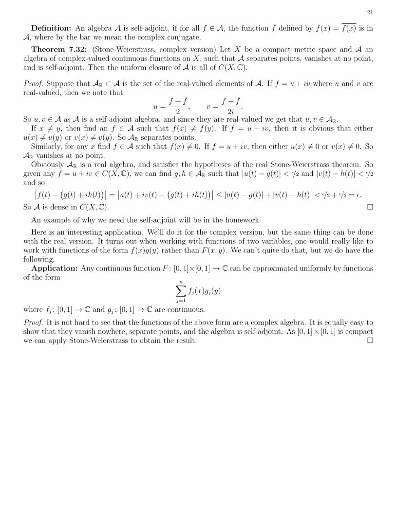
Definition: An algebra A is self-adjoint, if for all f ∈ A, the function f defined by f(x) = f(x) is inA, where by the bar we mean the complex conjugate.

Theorem 7.32: (Stone-Weierstrass, complex version) Let X be a compact metric space and A analgebra of complex-valued continuous functions on X, such that A separates points, vanishes at no point,and is self-adjoint. Then the uniform closure of A is all of C(X,C).

Proof. Suppose that AR ⊂ A is the set of the real-valued elements of A. If f = u + iv where u and v arereal-valued, then we note that

u =f + f

2, v =

f − f2i

.

So u, v ∈ A as A is a self-adjoint algebra, and since they are real-valued we get that u, v ∈ AR.If x 6= y, then find an f ∈ A such that f(x) 6= f(y). If f = u + iv, then it is obvious that either

u(x) 6= u(y) or v(x) 6= v(y). So AR separates points.Similarly, for any x find f ∈ A such that f(x) 6= 0. If f = u+ iv, then either u(x) 6= 0 or v(x) 6= 0. SoAR vanishes at no point.

Obviously AR is a real algebra, and satisfies the hypotheses of the real Stone-Weierstrass theorem. Sogiven any f = u+ iv ∈ C(X,C), we can find g, h ∈ AR such that |u(t)− g(t)| < ε/2 and |v(t)− h(t)| < ε/2and so∣∣f(t)−

(g(t) + ih(t)

)∣∣ =∣∣u(t) + iv(t)−

(g(t) + ih(t)

)∣∣ ≤ |u(t)− g(t)|+ |v(t)− h(t)| < ε/2 + ε/2 = ε.

So A is dense in C(X,C). �

An example of why we need the self-adjoint will be in the homework.

Here is an interesting application. We’ll do it for the complex version, but the same thing can be donewith the real version. It turns out when working with functions of two variables, one would really like towork with functions of the form f(x)g(y) rather than F (x, y). We can’t quite do that, but we do have thefollowing.

Application: Any continuous function F : [0, 1]×[0, 1]→ C can be approximated uniformly by functionsof the form

n∑j=1

fj(x)gj(y)

where fj : [0, 1]→ C and gj : [0, 1]→ C are continuous.

Proof. It is not hard to see that the functions of the above form are a complex algebra. It is equally easy toshow that they vanish nowhere, separate points, and the algebra is self-adjoint. As [0, 1]× [0, 1] is compactwe can apply Stone-Weierstrass to obtain the result. �