Lecture Notes 4: Fourier Series and PDE’s

1. Periodic Functions

A function f(x) defined on R is called a periodic function if there existsa number T > 0 such that

f(x+ T ) = f(x), ∀x ∈ R. (1.1)

The smallest number T for which the relation (1.1) holds is called the pe-riod of f or fundamental period of f .

Lemma 1.1. If f is T - periodic continuous function, then∫ a+T

a

f(x)dx =

∫ T

0

f(x)dx. (1.2)

Proof. Consider the function

F (x) =

∫ x+T

x

f(s)ds

It is clear that

F ′(x) = f(x+ T )− f(x) = 0,∀x ∈ R (f is T- periodic)

Thus F (x) is a constant function. Hence

F (a) =

∫ a+T

a

f(x)dx =

∫ T

0

f(x)dx = F (0).

�

2. Functional Series

Let

f1(x), f2(x), ..., fn(x), ... (2.1)

be a sequence of functions defined on some interval I ⊂ R. We say that thesequence (3.1) is convergent (or pointwise convergent) to a function f(x)on I if for each fixed point x ∈ I the number sequence {fn(x)} convergesto the number f(x). If at least for one point x0 the sequence f(x0) isdivergent, then we say that the sequence of functions {fn(x)} is divergenton I. .

1

2

A sequence of functions (3.1) is said to be uniformly convergent to a func-tion f(x) on I if for each ε > 0 there exists a number Nε depending on εonly, such that

|fn(x)− f(x)| ≤ ε

for all n ≥ Nε.

For a given sequence of functions (3.1) the series∞∑n=1

fn(x) (2.2)

is the following limitlimN→∞

SN(x),

whereSN(x) = f1(x) + f2(x) + ...+ fN(x)

is called the N -th partial sum of the series.If the sequence of partial sums {SN(x)} converges to some function s(x)on I, i.e.

∞∑n=1

fn(x) = s(x) (2.3)

, then we say that the series (3.8) is convergent on I to s(x). Otherwisethe series (3.8) is called divergent.If the sequence {SN(x)} is uniformly convergent to s(x) then we say thatthe series (3.8) is uniformly convergent.

Theorem 2.1. If the functions

f1(x), f2(x), ..., fn(x), ...

are continuous on an interval [a, b] and the series∞∑n=1

fn(x) is uniformly

convergent on [a, b], then the sum of the series s(x) is a continuous functionon [a, b]. Moreover the series obtained term by term integration of thisseries is also convergent and

∞∑n=1

∫ b

a

fn(x)dx =

∫ b

a

s(x)dx.

3

Theorem 2.2. (Weierstrass Theorem) If the functions

f1(x), f2(x), ..., fn(x), ...

are continuous on an interval [a, b],

|fn(x)| ≤ an, ∀x ∈ [a, b], n = 1, 2, ...

and the series∞∑n=1

an is convergent then the series∞∑n=1

fn(x) is uniformly

convergent to some function that is continuous on [a, b].

3. Euler’s formulas and Fourier series

A series of the form

a0

2+∞∑n=1

(an cos(nx) + bn sin(nx)) (3.1)

is called a trigonometric series.

Question: Which functions have trigonometric series expansion . Iff(x) has a trigonometric series expansion

f(x) =a0

2+∞∑n=1

(an cos(nx) + bn sin(nx)) (3.2)

how to compute a0, a1, ..., an, ..., b1, b2, ...?

Theorem 3.1. Suppose that f is 2π-periodic function and

f(x) =a0

2+∞∑n=1

(an cos(nx) + bn sin(nx)), (3.3)

where the series is converges uniformly on the real axis. Then

an =1

π

∫ π

−πf(x) cos(nx)dx, n = 0, 1, 2... (3.4)

bn =1

π

∫ π

−πf(x) sin(nx)dx, n = 1, 2... (3.5)

4

Proof. Really since∫ π

−πcos(nx)dx = 0,

∫ π

−πsin(nx)dx = 0

and due to uniform convergence of the series we can integrate (3.1) over(−π, π) and get: ∫ π

−πf(x)dx = a0π,

Let us multiply (3.1) by cos(mx) and integrate over (−π, π). Taking intoaccount ∫ π

−πcos2(mx)dx = π,

∫ π

−πsin2(mx)dx = π

we obtain

an =1

π

∫ π

−πf(x) cos(nx)dx, n = 0, 1, 2... (3.6)

bn =1

π

∫ π

−πf(x) sin(nx)dx, n = 1, 2... (3.7)

Here we have used the fact that for eachm the series cos(mx)∑∞

n=1(an cos(nx)+bn sin(nx)) and sin(mx)

∑∞n=1(an cos(nx) + bn sin(nx)) are uniformly con-

vergent. �

The series (3.1) where an and bn are defined by (3.6) and (3.7) is called theFourier series of the function f , the numbers an, bn are called the Fouriercoefficients of f .Piecewise continuous function. A function f(x) is called piecewisecontinuous on [a, b], if limx→b− f(x), limx→a+ f(x) exist f is continuous on(a, b) except at finitely many of points in (a, b), where f has one-sidedlimits.

Theorem 3.2. If 2π-periodic function f(x) and its derivative f ′(x) arepiecewise continuous functions, then

f(x+) + f(x−)

2=a0

2+∞∑n=1

(an cos(nx) + bn sin(nx)) (3.8)

for each x ∈ R, where an and bn are defined by (3.4) and (3.5).

5

Example 3.3. Consider the function Φ(x) given on [−π, π] by

φ(x) =

{π + x, x ∈ [−π, 0]

π − x, x ∈ [0, π].

φ(x) is piecewise smooth.

a0 =1

π

∫ π

−πφ(x)dx =

2

π

∫ π

0

(π − x)dx =2

π

[πx− x2

2

]π0

= 2π − π = π

an =2

π

∫ π

0

(π − x) cos(nx)dx == 2

∫ π

0

cos(nx)dx− 2

π

∫ π

0

x cos(nx)dx

= −2

π

∫ π

0

x

(1

nsin(nx)

)′dx = − 2

nπ[x sin(nx)]π0 +

2

nπ

∫ π

0

sin(nx)dx

=2

nπ

[−1

ncos(nx)

]π0

=2

nπ

[1

n− 1

ncos(nπ)

]=

2

nπ

1

n2− (−1)n

n2

Thus an = 0 if n is and even number, and an = 2n2 , if n is and odd number.

φ(x) =π

2+

4

π

∞∑k=1

1

(2k − 1)2cos(2k − 1)x

Example 3.4. Using Fourier series show that

π2

8= 1 +

1

32+

1

52+

1

72+ ...

3.1. Functions of any period p = 2l.

f(x) =a0

2+∞∑n=1

(an cos

(nπlx)

+ bn sin(nπlx))

(3.9)

an =1

l

∫ l

0

f(x) cos(nπlx)dx, bn =

1

l

∫ l

0

f(x) sin(nπlx)dx. (3.10)

3.2. Even and Odd Functions. If a function f(x) is an even function ,then

bn =2

l

∫ l

0

f(x) sin(nπlx)dx = 0

6

and its Fourier series has the form

f(x) =a0

2+∞∑n=1

an cos(nπlx), (3.11)

where

an =2

l

∫ l

0

f(x) cos(nπlx)dx, n = 0, 1, 2, ... (3.12)

If a function f(x) is an odd function , then

an =2

l

∫ l

0

f(x) cos(nπlx)dx = 0

and its Fourier series has the form

f(x) =∞∑n=1

bn sin(nπlx)x, (3.13)

where

bn =2

l

∫ l

0

f(x) sin(nπlx)dx, n = 1, 2, ... (3.14)

Let f(x) be defined on [0, l]. We define the even periodic extension fe off as follows

fe(x) = f(−x), if x ∈ [−l, 0], and fe(x) = fe(x+ 2l),∀x ∈ R.

An odd periodic extension f0 of f is defined as follows

f0(x) = −f(−x), if x ∈ [−l, 0], and f0(x) = f0(x+ 2l),∀x ∈ R.

Example 3.5. Find Fourier series expansion for f(x) = 1−x2, x ∈ [−1, 1].

a0 = 2

∫ 1

0

(1− x2)dx =4

3,

an = 2

∫ 1

0

(1− x2) cos(nπx)dx = −2

∫ 1

0

cos(nπx)dx+

2

∫x2

(1

nπsin(nπx

)′dx = − 2

nπ

∫ 1

0

2x sin(nπx)dx =

4

nπ

∫ 1

0

x

(− 1

nπcos(nπx

)′dx = − 4

(nπ)2x cos(nπx)|10 = − 4

n2π2(−1)n.

7

Thus we have

f(x) =2

3+

4

π2

∞∑n=1

(−1)n+1

n2cos(nπx).

4. Riemann -Lebesgue Lemma

Proposition 4.1. If f(x) is a continuous function , then

limn→∞

In = limn→∞

∫ π

−πf(x) cos(nx)dx = 0,

limn→∞

Jn = limn→∞

∫ π

−πf(x) sin(nx)dx = 0. (4.1)

Proof of 4.1. Since cosα = − cos(α+ π) we have

In :=

∫ π

−πf(x) cos(nx)dx = −

∫ π

−πf(x) cos

[(x+

π

n)n]dx.

Making change of variables x+ πn = y and using the Lemma 1.1 we obtain

∫ π

−πf(x) cos(nx)dx = −

∫ π+π2

−π+π2

f(y − π

n) cos(ny)dy = −

∫ π

−πf(y − π

n) cos(ny)dy

Hence we have

In + In = 2

∫ π

−πf(x) cos(nx)dx =

∫ π

−π[f(x)− f(x− π

n)] cos(nx)dx

= 2

∣∣∣∣∫ π

−πf(x) cos(nx)dx

∣∣∣∣ ≤ ∫ π

−π|f(x)− f(x− π

n)|dx.

The function f is continuous on [−π, π] thus it is uniformly continuous on [−π, π]. Therefore the

integral in the right hand side of (R) tends to zero as n → ∞. So In → 0 as n → ∞. Similarly

we can show that Jn → 0 as n→∞.

Problem. Let f(x) be 2π -periodic and f ′(x) is continuous function. Showthat

an = o

(1

n

), bn = o

(1

n

).

8

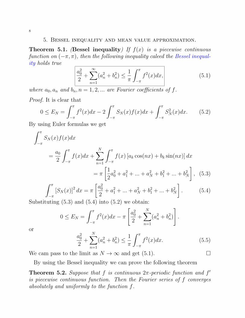
5. Bessel inequality and mean value approximation.

Theorem 5.1. (Bessel inequality) If f(x) is a piecewise continuousfunction on (−π, π), then the following inequality caleed the Bessel inequal-ity holds true

a20

2+∞∑n=1

(a2n + b2

n) ≤1

π

∫ π

−πf 2(x)dx, (5.1)

where a0, an and bn, n = 1, 2, ... are Fourier coefficients of f .

Proof. It is clear that

0 ≤ EN =

∫ π

−πf 2(x)dx− 2

∫ π

−πSN(x)f(x)dx+

∫ π

−πS2N(x)dx. (5.2)

By using Euler formulas we get∫ π

−πSN(x)f(x)dx

=a0

2

∫ π

−πf(x)dx+

N∑n=1

∫ π

−πf(x) [ak cos(nx) + bk sin(nx)] dx

= π

[1

2a2

0 + a21 + ...+ a2

N + b21 + ...+ b2

N

], (5.3)∫ π

−π[SN(x)]2 dx = π

[a2

0

2+ a2

1 + ...+ a2N + b2

1 + ...+ b2N

]. (5.4)

Substituting (5.3) and (5.4) into (5.2) we obtain:

0 ≤ EN =

∫ π

−πf 2(x)dx− π

[a2

0

2+

N∑n=1

(a2n + b2

n)

].

ora2

0

2+

N∑n=1

(a2n + b2

n) ≤1

π

∫ π

−πf 2(x)dx. (5.5)

We cam pass to the limit as N →∞ and get (5.1). �

By using the Bessel inequality we can prove the following theorem

Theorem 5.2. Suppose that f is continuous 2π-periodic function and f ′

is piecewise continuous function. Then the Fourier series of f convergesabsolutely and uniformly to the function f .

9

Proof. Let us calculate the Fourier coefficients of f ′:

α0 =1

π

∫ π

−πf ′(x)dx =

1

π(f(π)− f(−π)) = 0,

αn =1

π

∫ π

−πf ′(x) cos(nx)dx =

1

πcos(nx)f(x)

∣∣∣x=π

x=−π+n

∫ π

−πf(x) sin(nx)dx = nbn,

βn =1

π

∫ π

−πf ′(x) sin(nx)dx

=1

πsin(nx)f(x)

∣∣∣x=π

x=−π− n

∫ π

−πf(x) cos(nx)dx = nan.

So we have

αn = nbn, n = 0, 1, 2, ..., βn = nan, n = 1, 2, ..., (5.6)

Employing the inequality

|ab| ≤ 1

4a2 + b2

we obtain from (5.6) the following inequlity

|an|+ |bn| =1

n|βn|+

1

n|αn| ≤

1

2n2+ α2

n + β2n.

Due to the Bessel inequality the series

∞∑n=1

(α2n + β2

n)

is convergent. Hence the series∑∞

n=1(|an|+ |bn|) is also convergent. There-fore the series

a0

2+∞∑n=1

(an cos

nπ

lx+ bn sin

nπ

lx)

is uniformly convergent to a continuous function f .�

where an and bn are Fourier coefficients of the function f

10

Example 5.3. Assume that the Fourier series of f(x) on [−π, π] convergesto f(x) and can be integrated term by term. Multiply

a0

2+∞∑n=1

(an cos

nπ

lx+ bn sin

nπ

lx)

by f(x) and integrate the obtained relation from −π to π to derive theidentity

1

π

∫ π

−πf 2(x)dx =

a20

2+∞∑n=1

(a2n + b2

n). (5.7)

This identity is called the Parseval identity.

6. Heat Equation. Method of Separation of Variables

We consider the problem

ut = a2uxx, x ∈ (0, l), t > 0, (6.1)

u(x, 0) = f(x), x ∈ [0, l], (6.2)

u(0, t) = u(l, t) = 0, t ≥ 0, (6.3)

We assume that the solution of the problem has the form

u(x, t) = X(x)T (t),

where X(x) and T (t) are nonzero functions. Substituting into (6.1) we get

X(x)T ′(t) = a2X ′′(x)T (t).

Dividing both sides of the last equality by a2X(x)T (t) we obtain

T ′(t)

a2T (t)=X ′′(x)

X(x)(6.4)

Since the left hand side of (6.4) depends only on t and the right handside depend only on x each side of this equality can only be equal to someconstant. Thus

T ′(t)

a2T (t)=X ′′(x)

X(x)= −λ, λ = constant

orT ′(t) = λa2T (t) (6.5)

X ′′(x) + λX(x) = 0. (6.6)

11

It follows from (3) thatX(0) = X(l) = 0. (6.7)

So we have to find the values of λ for which the equation (6.6) has nonzerosolution which satisfy (6.7). The values of l for which (6.6) has nonzerosolution satisfying (6.7) are called eigenvalues of the problem (6.6),(6.7)When l = 0 (6.7), the corresponding solutions - eigenfunctions of (6.6),(6.7).When l = 0 the equation has a general solution

X(x) = Ax+B

This function satisfies (6.7) just for A = B = 0. Thus λ = 0 is not aneigenvalue.If λ < 0 then general solution of (6.6) has the form

X(x) = C1e√|λ|x + C1e

−√|λ|x.

It is easy to see that this function satisfies (6.7) just when C1 = C2 = 0.So (6.6),(6.7) has not negative eigenvalues.If l > 0 then the general solution of (6.6) has the form

X(x) = C1 cos(√λx) + C2 sin(

√λx).

Substituting into (6.7) we obtain

X(0) = C1 = 0, X(l) = C2 sin(√λl) = 0

The second equality holds for ll = nπ, n = ±1,±2, ... Thus the numbers

λn =n2π2

l2, n = 1, 2, ...

are eigenvalues of the problem (6.6),(6.7), and the functions

Xn(x) = sin(nπlx), n = 1, 2, ...

are the corresponding eigenfunctions. It is easy to see that the generalsolution of (6.5) for l = ln has the form

Tn(t) = Dne−a2λnt, n = 1, 2, ...

Hence for each n = 1, 2, ... the function e−a2λnt sin

(nπl x)

satisfies (6.1),(6.3).Since the equation (6.6) is a linear equation for each N

uN(x, t) =N∑n=1

Dne−a2λnt sin

(nπlx), (6.8)

12

where Dn, n = 1, ..., N are arbitrary constants also satisfies (6.1),(6.3).Next we try to satisfy the initial condition (6.2):

uN(x, 0) =N∑n=1

Dn sin(nπlx)

= f(x)

We see that the solution of the problem (6.1)-(6.3) has this form just whenthe initial function is linear combination of functions

sin√λ1x, ...., sin

√λnx, λk =

k2π2

l2.

Let us consider the series

u(x, t) =∞∑n=1

Dne−a2λnt sin

(nπlx). (6.9)

Let us note that if∞∑n=1|Dn| <∞ , then this series is uniformly convergent

on [−l, l] × [0, T ],∀T > 0. The function u(x, t) defined by (6.9) satisfiesthe boundary conditions (6.3) since each term of the series satisfies theseconditions. It follows from (6.9) that u(x, t) satisfies the initial condition(6.2)

f(x) = u(x, 0) =∞∑n=1

Dn sin(nπlx)

(6.10)

iff

Dn = fn =2

l

∫ l

0

f(x) sin(nπlx)dx.

Theorem 6.1. If f(x) is continuous on [0, L], f ′(x) is piecewise continuouson [0, L], f(0) = f(l) = 0 then the function

u(x, t) =∞∑n=1

fne−a2λnt sin

(nπlx)

(6.11)

satisfies (6.1)-(6.3).

To prove this theorem we need the following proposition

Proposition 6.2. Assume that the functions vn(x, t), n = 1, 2, ... are continuous QT = [a, b] ×[t0, T ] and

|vn(x, t)| ≤ an,∀(x, t) ∈ QT , n = 1, 2, ...

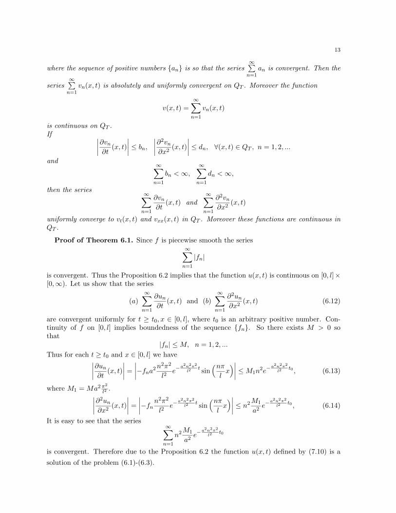
13

where the sequence of positive numbers {an} is so that the series∞∑n=1

an is convergent. Then the

series∞∑n=1

vn(x, t) is absolutely and uniformly convergent on QT . Moreover the function

v(x, t) =∞∑n=1

vn(x, t)

is continuous on QT .If ∣∣∣∣∂vn∂t (x, t)

∣∣∣∣ ≤ bn, ∣∣∣∣∂2vn∂x2(x, t)

∣∣∣∣ ≤ dn, ∀(x, t) ∈ QT , n = 1, 2, ...

and∞∑n=1

bn <∞,∞∑n=1

dn <∞,

then the series∞∑n=1

∂vn∂t

(x, t) and∞∑n=1

∂2vn∂x2

(x, t)

uniformly converge to vt(x, t) and vxx(x, t) in QT . Moreover these functions are continuous inQT .

Proof of Theorem 6.1. Since f is piecewise smooth the series∞∑n=1

|fn|

is convergent. Thus the Proposition 6.2 implies that the function u(x, t) is continuous on [0, l]×[0,∞). Let us show that the series

(a)∞∑n=1

∂un∂t

(x, t) and (b)∞∑n=1

∂2un∂x2

(x, t) (6.12)

are convergent uniformly for t ≥ t0, x ∈ [0, l], where t0 is an arbitrary positive number. Con-tinuity of f on [0, l] implies boundedness of the sequence {fn}. So there exists M > 0 sothat

|fn| ≤M, n = 1, 2, ...

Thus for each t ≥ t0 and x ∈ [0, l] we have∣∣∣∣∂un∂t (x, t)

∣∣∣∣ =

∣∣∣∣−fna2n2π2l2e−

a2n2π2

l2t sin

(nπlx)∣∣∣∣ ≤M1n

2e−a2n2π2

l2t0 , (6.13)

where M1 = Ma2 π2

l2.∣∣∣∣∂2un∂x2(x, t)

∣∣∣∣ =

∣∣∣∣−fnn2π2l2e−

a2n2π2

l2t sin

(nπlx)∣∣∣∣ ≤ n2M1

a2e−

a2n2π2

l2t0 , (6.14)

It is easy to see that the series∞∑n=1

n2M1

a2e−

a2n2π2

l2t0

is convergent. Therefore due to the Proposition 6.2 the function u(x, t) defined by (7.10) is a

solution of the problem (6.1)-(6.3).

14

Problem 6.3. Let the series∞∑n=1

a2n and

∞∑n=1

b2n be convergent. Show that

∞∑n=1

|anbn| ≤

( ∞∑n=1

a2n

)1/2( ∞∑n=1

b2n

)1/2

6.1. Nonhomogeneous Equation.

ut = a2uxx + h(x, t), x ∈ (0, l), t > 0, (6.15)

u(x, 0) = f(x), x ∈ [0, l], (6.16)

u(0, t) = u(l, t) = 0, t ≥ 0, (6.17)

We look for solution of the problem (6.15)-(6.17) in the form

u(x, t) =∞∑n=1

un(t) sin(nπlx)

(6.18)

We expand h(x, t)

h(x, t) =∞∑n=1

hn(t) sin(nπlx)

By using (6.18) we obtain from (6.15)∞∑n=1

[u′n(t) + λna

2un(t)− hn(t)]

sin(√λnx) = 0.

This equality holds iff

u′n(t) + λna2un(t) = hn(t), n = 1, 2, ... (6.19)

Taking into accoun the initial condition (6.16) we obtain

u(x, 0) =∞∑n=1

hn(0) sin(nπl

)x = f(x) =

∞∑n=1

fn sin(nπl

)x.

It follows then

un(0) = fn, n = 1, 2, ... (6.20)

The initial value problem (6.19),(6.21) has the solution

un(t) = e−λna2tfn +

∫ t

0

e−λna2(t−s)hn(s)ds

15

Inserting the expression for un(t) into (6.18) we get

u(x, t) =∞∑n=1

[fne−λna2t +

∫ t

0

e−λna2(t−s)hn(s)ds

]sin(nπl

)x. (6.21)

Let us recall that λn = n2π2

l2 .

Problem 6.4. Show that the problem (6.1)-(6.3) has a unique solution.

Hint. Assume that v(x, t) is another solution of this problem, i.e.

vt = a2vxx, x ∈ (0, l), t > 0,

v(x, 0) = f(x), x ∈ [0, l],

v(0, t) = v(l, t) = 0, t ≥ 0,

Then show that the function

w(x, t) = u(x, t)− v(x, t)

which is a solution of the problem

wt = a2wxx, x ∈ (0, l), t > 0,

w(x, 0) = 0, x ∈ [0, l],

w(0, t) = w(l, t) = 0, t ≥ 0

satisfies1

2

d

dt

∫ l

0

[w(x, t)]2dx+ a2

∫ l

0

[wx(x, t)]2dx = 0.

6.2. Nonhomogeneous boundary conditions. Let us consider the prob-lem

ut = a2uxx, x ∈ (0, l), t > 0, (6.22)

u(x, 0) = f(x), x ∈ [0, l], (6.23)

u(0, t) = A, u(l, t) = B, t ≥ 0, (6.24)

where A,B are given constants. The solution of the problem u(x, t) isa summ of two functions v(x, t and W (x), where W is a solution of theproblem {

W ′′(x) = 0, x ∈ (0, l),

W (0) = A, W (l) = B(6.25)

16

and v is a solution of the problemvt = a2vxx, x ∈ (0, l), t > 0,

v(x, 0) = f(x)−W (x), x ∈ [0, l],

u(0, t) = u(l, t) = 0, t ≥ 0,

(6.26)

It is clear that

W (x) = A+1

l(B − A)x

is a solution of the problem (6.25) Hence the solution of the proble (6.27)-(6.29) is the function

u(x, t) =∞∑n=1

qne−n2a2t sin

(nπlx)

+ A+1

l(B − A)x,

where

qn =2

l

∫ l

0

(f(x)− A− 1

l(B − A)x

)sin(nπlx).

Next we consider the following problem

ut = a2uxx, x ∈ (0, l), t > 0, (6.27)

u(x, 0) = f(x), x ∈ [0, l], (6.28)

u(0, t) = φ(t), u(l, t) = ψ(t), t ≥ 0, (6.29)

we look the solution of the problem(6.27)-(6.29) in the form

u(x, t) =∞∑n=1

un(t) sin(√

λnx)

(6.30)

For ut we have

ut(x, t) =∞∑n=1

u′n(t) sin(√

λnx)

(6.31)

uxx(x, t) =

∞∑n=1

gn(t) sin(√

λnx), (6.32)

where

gn(t) =2

l

∫ l

0uxx(x, t) sin

(√λnx

)dx.

17

Integrating by parts we obtain

gn(t) =2

l

[ux sin

(√λnx

)]l0− 2

l

√λn

∫ l

0ux(x, t) cos

(√lnx)dx

= −[

2

l

√λnu(x, t) cos

(√λnx

)]l0

− 2

lλn

∫ l

0u(x, t) sin

(√λnx

)dx

=2

l

√λn[u(0, t)− u(l, t) cos(nπ)]− λnun(t).

Employing the boundary conditions (6.29) we obtain

gn(t) =2

l

√λn[φ(t)− ψ(t) cos(nπ)]− λnun(t)

Thus (6.32) implies

uxx(x, t) =

∞∑n=1

[2√λnl

φ(t)− 2√λnl

(−1)nψ(t)− lnun(t)

]sin(√

λnx)

By using the last relation and (6.31) in(6.27) we obtain

∞∑n=1

[u′n(t)− a2

(2a2√λn

lφ(t)− 2a2

√λn

l(−1)nψ(t)− aλnun(t)

)]sin(√

λnx)

= 0.

Therefore the Fourier coefficients un(t) satisfy

u′n(t) = a2[

2√λnl

φ(t)− 2√λnl

(−1)nψ(t)− λnun(t)

], n = 1, 2, ... (6.33)

The function u will satisfy the initial condition (6.28) iff

un(0) = fn, n = 1, 2, ... (6.34)

We solve the initial value problem (6.33),(6.34) and get

un(t) = fne−a2λnt − 2a2

√λn

l

∫ t

0e−a

2λn(t−s) [(−1)nψ(s)− φ(s)] ds, n = 1, 2, ... (6.35)

So the solution of the problem (6.27)-(6.29) has the form (6.30), where un(t), n = 1, 2, ... are

defined by (6.35)

7. Wave Equation

In this section we study the wave equation. The first problem is the initialboundary value problem:

utt = c2uxx, x ∈ (0, l), t > 0, (7.1)

u(x, 0) = f(x), ut(x, 0) = g(x), x ∈ [0, l], (7.2)

u(0, t) = u(l, t) = 0, t ≥ 0, (7.3)

We assume that the solution of the problem has the form

u(x, t) = X(x)T (t),

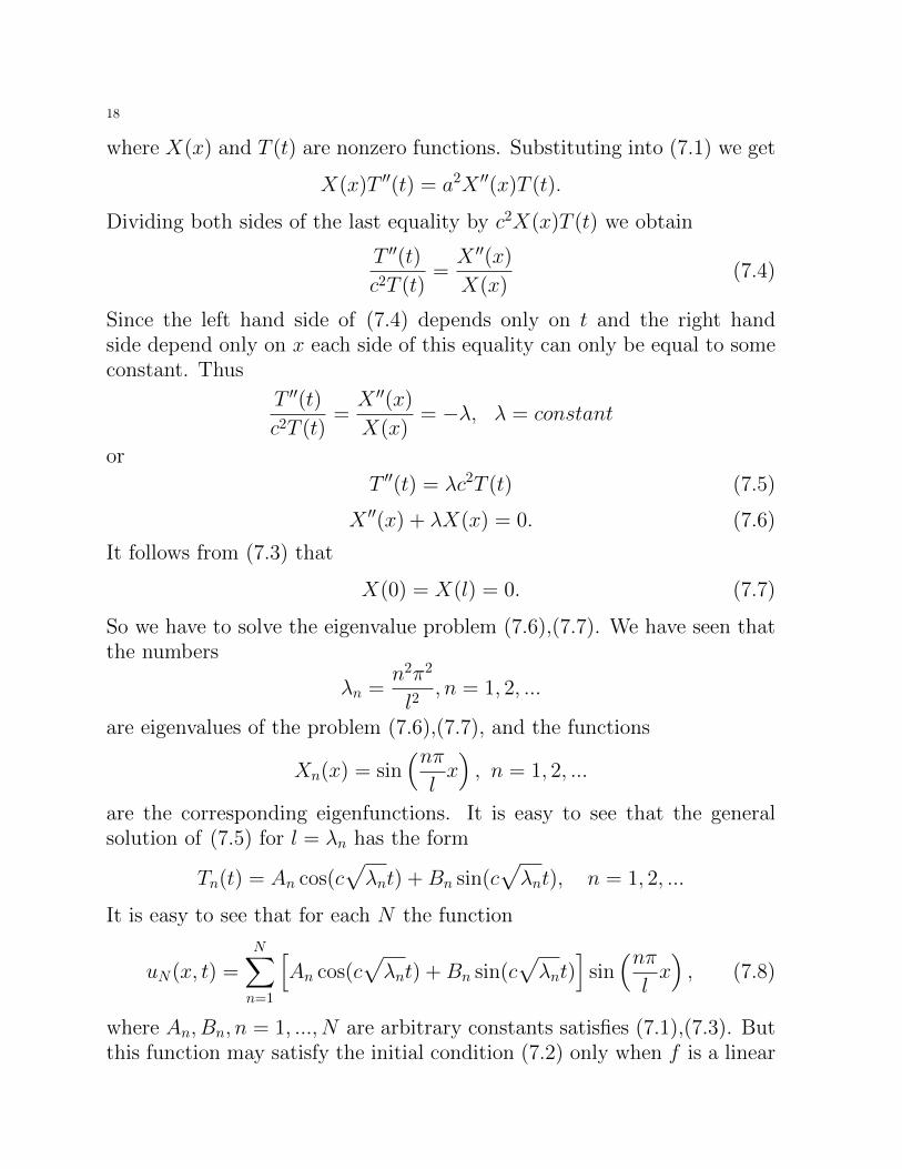
18

where X(x) and T (t) are nonzero functions. Substituting into (7.1) we get

X(x)T ′′(t) = a2X ′′(x)T (t).

Dividing both sides of the last equality by c2X(x)T (t) we obtain

T ′′(t)

c2T (t)=X ′′(x)

X(x)(7.4)

Since the left hand side of (7.4) depends only on t and the right handside depend only on x each side of this equality can only be equal to someconstant. Thus

T ′′(t)

c2T (t)=X ′′(x)

X(x)= −λ, λ = constant

or

T ′′(t) = λc2T (t) (7.5)

X ′′(x) + λX(x) = 0. (7.6)

It follows from (7.3) that

X(0) = X(l) = 0. (7.7)

So we have to solve the eigenvalue problem (7.6),(7.7). We have seen thatthe numbers

λn =n2π2

l2, n = 1, 2, ...

are eigenvalues of the problem (7.6),(7.7), and the functions

Xn(x) = sin(nπlx), n = 1, 2, ...

are the corresponding eigenfunctions. It is easy to see that the generalsolution of (7.5) for l = λn has the form

Tn(t) = An cos(c√λnt) +Bn sin(c

√λnt), n = 1, 2, ...

It is easy to see that for each N the function

uN(x, t) =N∑n=1

[An cos(c

√λnt) +Bn sin(c

√λnt)

]sin(nπlx), (7.8)

where An, Bn, n = 1, ..., N are arbitrary constants satisfies (7.1),(7.3). Butthis function may satisfy the initial condition (7.2) only when f is a linear

19

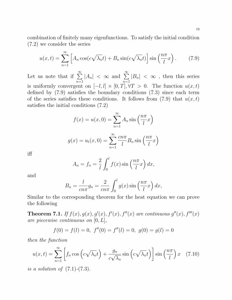
combination of finitely many eigenfunctions. To satisfy the initial condition(7.2) we consider the series

u(x, t) =∞∑n=1

[An cos(c

√λnt) +Bn sin(c

√λnt)

]sin(nπlx). (7.9)

Let us note that if∞∑n=1|An| < ∞ and

∞∑n=1|Bn| < ∞ , then this series

is uniformly convergent on [−l, l] × [0, T ],∀T > 0. The function u(x, t)defined by (7.9) satisfies the boundary conditions (7.3) since each termof the series satisfies these conditions. It follows from (7.9) that u(x, t)satisfies the initial conditions (7.2)

f(x) = u(x, 0) =∞∑n=1

An sin(nπlx)

g(x) = ut(x, 0) =∞∑n=1

cnπ

lBn sin

(nπlx)

iff

An = fn =2

l

∫ l

0

f(x) sin(nπlx)dx,

and

Bn =l

cnπgn =

2

cnπ

∫ l

0

g(x) sin(nπlx)dx,

Similar to the corresponding theorem for the heat equation we can provethe following

Theorem 7.1. If f(x), g(x), g′(x), f ′(x), f ′′(x) are continuous g′′(x), f ′′′(x)are piecewise continuous on [0, L],

f(0) = f(l) = 0, f ′′(0) = f ′′(l) = 0, g(0) = g(l) = 0

then the function

u(x, t) =∞∑n=1

[fn cos

(c√λnt)

+gn

c√λn

sin(c√λnt)]

sin(nπl

)x (7.10)

is a solution of (7.1)-(7.3).

20

7.1. Nonhomogeneous Equation.

utt = c2uxx + h(x, t), x ∈ (0, l), t > 0, (7.11)

u(x, 0) = f(x), ut(x, 0) = g(x), x ∈ [0, l], (7.12)

u(0, t) = u(l, t) = 0, t ≥ 0, (7.13)

We look for solution of the problem (7.11)-(7.13) in the form

u(x, t) =∞∑n=1

un(t) sin(nπlx)

(7.14)

We expand h(x, t)

h(x, t) =

∞∑n=1

hn(t) sin(nπlx)

By using (7.14) we obtain from (7.11)

∞∑n=1

[u′n(t) + λna

2un(t)− hn(t)]

sin(√λnx) = 0.

This equality hold iff

u′′n(t) + λnc2un(t) = hn(t), n = 1, 2, ... (7.15)

Taking into account the initial condition (7.12) we obtain

u(x, 0) =

∞∑n=1

An(0) sin(nπl

)x = f(x) =

∞∑n=1

fn sin(nπl

)x.

ut(x, 0) =

∞∑n=1

cnπ

lBn(0) sin

(nπl

)x = g(x) =

∞∑n=1

gn sin(nπl

)x.

It follows then

An(0) = fn, Bn(0) =l

cnπgn, n = 1, 2, ... (7.16)

The initial value problem (7.15),(7.16) has the solution

un(t) = fn cos(c√λnt)

+lgn

c√ln

sin(c√λnt)

+

∫ t

0sin[cnπl

(t− s)]hn(s)ds

Inserting the expression for un(t) into (7.14) we get

u(x, t) =∞∑n=1

[fn cos

(c√λnt)

+gn

c√λn

sin(c√λnt)]

sin(nπl

)x

+∞∑n=1

∫ t

0sin[c√λn(t− s)

]hn(s)ds sin

(nπl

)x (7.17)

Remember that λn = n2π2

l2.

Problem 7.2. Show that the problem (7.1)-(7.3) has a unique solution.

21

Hint. Assume that v is another solution of the problem. Then observethat w(x, t) satisfies

wtt = c2wxx, x ∈ (0, l), t > 0, (7.18)

w(x, 0) = 0, wt(x, 0) = 0, x ∈ [0, l], (7.19)

w(0, t) = w(l, t) = 0, t ≥ 0. (7.20)

Multiply the equation by wt, integrate the obtained relation with respectto x over the interval (0, l) and obtain the equality

d

dt

∫ l

0

([wt(x, t)]

2 + [wx(x, t)]2)dx = 0.

7.2. The Cauchy problem for the wave equation. Now we considerthe initial value problem for the wave equation, i.e. we would like to findsolution of the equation

utt = c2uxx, t > 0, x ∈ (−∞,∞), (7.21)

under the initial conditions

u(x, 0) = f(x); ut(x, 0) = g(x), x ∈ (−∞,∞), (7.22)

where f and g are given numbers and c > 0 is a given number. To solvethe problem we make the following change of variables

ξ = x− ct, η = x+ ct.

By using the chain rule we find

ut = uξξt + uηηt = −auξ + cuη = c(uη − uξ),

utt = c(uηξξt + uηηηt − uξξξt − uξηηt) = c2(uξξ − 2uξη + uηη), (7.23)

ux = uξξx + uηηx = uξ + uη,

uxx = uξξξx + uξηηx + uηξξx + uηηηx = uξξ + 2uξη + uηη (7.24)

Bu using (7.23) and (7.24) in (7.21) we find

uξη = 0. (7.25)

It is clear that for each differentiable functions u1, u2 the function

u(ξ, η) = u1(ξ) + u2(η),

isa solution of (7.25) . Hence the function

u(x, t) = u1(x− ct) + u2(x+ ct) (7.26)

22

is a solution of (7.21). Bu using the initial conditions (7.22) we get

u(x, 0) = u1(x) + u2(x) = f(x), (7.27)

ut(x, 0) = −cu′1(x) + cu′2(x) = g(x).

Integrating the last equality we obtain

u2(x)− u1(x) =1

c

∫ x

x0

g(s)ds+ C. (7.28)

Solving the system of equations (7.27), (7.28) we obtain

u1(x) =1

2f(x)− 1

2c

∫ x

x0

g(s)ds− C

2,

u2(x) =1

2f(x) +

1

2c

∫ x

x0

g(s)ds+C

2.

Iserting the values of u1, u2 from the last two equalities into (7.26) we get

u(x, t) =1

2ϕ(x− ct)− 1

2a

∫ x−ct

x0

g(s)ds+1

2f(x+ ct) +

1

2c

∫ x+ct

x0

g(s)ds

or

u(x, t) =f(x− ct) + f(x+ ct)

2+

1

2a

∫ x+ct

x−ctg(s)ds, (7.29)

The last equality is called the D’Alembert formula .