Embed Size (px)
Citation preview

Lecture Notes on DSF 2021
1
LECTURE NOTE
DYNAMICS OF SOILS AND FOUNDATIONS
SECOND SEMESTER
M.TECH (GTE)
Dr. Debabrata Giri, Associate Professor
Department of Civil Engineering
Veer Surendra Sai University of Technology, Burla
Email: [email protected]

Lecture Notes on DSF 2021
2
DISCLAIMER
These lecture notes are being prepared and printed for the use in training
the students. No commercial use of these notes is permitted and copies
of these will not be offered for sale in any manner. This lecture notes
will provide the basic knowledge about the course. The students are
advised to refer Text and Reference books to gather more knowledge.
The readers are encouraged to provide written feedbacks for
improvement of course materials.
Dr. Debabrata Giri

Lecture Notes on DSF 2021
3
Subject Name: DYNAMICS OF SOILS AND FOUNDATIONS MCEGT201
Course Content
Module-I
Fundamentals of vibrations: single, two and multiple degree of freedom systems,
vibration isolation, vibration absorbers, vibration measuring instruments.
Module-II
Wave propagation: elastic continuum medium, semi-infinite elastic continuum
medium, soil behaviour under dynamic loading.
Module-III
Liquefaction of soils: liquefaction mechanism, factors affecting liquefaction, studies by
dynamic tri-axial testing, shake table and blast tests, assessment of liquefaction potential.
Module-IV
Dynamic elastic constants of soil: determination of dynamic elastic constants, various
methods including block resonance tests, cyclic plate load tests, wave propagation tests,
oscillatory shear box test.
Module-V
Theory of Vibration of Foundation: Vertical, sliding, torsional and rocking oscillation of
footing resting on Elastic half space. Oscillation of rigid circular footing supported by an
elastic layer. Introduction of bearing capacity of dynamically loaded shallow foundation.
Reference Books:
Das, B.M., “Fundamentals of Soil Dynamics”, Elsevier, 1983.
Steven Kramer, “Geotechnical Earthquake Engineering”, Pearson, 2008.
Prakash, S., Soil Dynamics, McGraw Hill, 1981.
Kameswara Rao, N.S.V., Vibration analysis and foundation dynamics, Wheeler
Publication Ltd., 1998.
Richart, F.E. Hall J.R and Woods R.D., Vibrations of Soils and Foundations, Prentice Hall
Inc., 1970.
Prakash, S. and Puri, V.K., Foundation for machines: Analysis and Design, John Wiley &
Sons, 1998
COURSE OUTCOME
Students can interpret theory of vibration and resonance phenomenon, dynamic
amplification.
Students can investigate propagation of body waves and surface waves through soil.
Students can predict dynamic bearing capacity and assess liquefaction potential of any site.
Student exposed to different methods for estimation of dynamic soil properties required for
design purpose.
Students apply theory of vibrations to design machine foundation based on dynamic soil
properties and bearing capacity

Lecture Notes on DSF 2021
4
1.0 FUNDAMETALS OF VIBRATION
In order to understand the behaviour of a structure subjected to dynamic load lucidly, one must
study the mechanics of vibrations 'caused by the dynamic load. The pattern of variation of a
dynamic load with respect to time may be either periodic or transient. The periodical motions can
be resolved into sinusoidally varying components e.g. vibrations in the case of reciprocating
machine foundations. Transient vibrations may have very complicated non-periodic time history
e.g. vibrations due to earthquakes and quarry blasts.
A structure subjected to a dynamic load (periodic or transient) may vibrate in one of the
following four ways of deformation or a combination there-of:
(i) Extensional
(ii) Bending
(iii) Shearing
(iv) Torsional
The forms of vibration mainly depend on the mass, stiffness distribution and end conditions of
the system.
To study the response of a vibratory system, in many cases it is satisfactory to reduce it to an
idealized system of lumped parameters. In this regard, the simplest model consists of mass,
spring and dashpot. This chapter is framed to provide the basic concepts and dynamic analysis of
such systems. Actual field problems which can be idealized to mass-spring-dashpot systems,
have also been included.
1.1 Important Definition
Vibrations: If the motion of the body is oscillatory in character, it is called vibration.
Degrees of Freedom: The number of independent co-ordinates which are required to define the
position of a system during vibration, is called degrees of freedom (Fig. 1)
Periodic Motion: If motion repeats itself at regular intervals of time, it is called periodic motion.
Free Vibration: If a system vibrates without an external force, then it is said to undergo free
vibrations. Such vibrations can be caused by setting the system in motion initially and allowing it
to move.
Natural Frequency: This is the property of the system and corresponds to the number of free
oscillations made by the system in unit time.
Forced Vibrations: Vibrations that are developed by externally applied exciting forces are called
forced vibrations. These vibrations occur at the frequency of the externally applied exciting
force.
Forcing Frequency: This refers to the periodicity of the external forces which acts on the system
during forced vibrations. This is also termed as operating frequency.
Frequency Ratio: The ratio of the forcing frequency and natural frequency of the system is
referred as frequency ratio.
Amplitude of Motion: The maximum displacement of a vibrating body from the mean position is
amplitude of motion.
Time Period: Time taken to complete one cycle of vibration is known as time period.

Lecture Notes on DSF 2021
5
Resonance: A system having n degrees of freedom has n natural frequencies. If the frequency of
excitation coincides with anyone of the natural frequencies of the system, the condition of
resonance occurs. The amplitudes of motion are very excessive at resonance.
Fig.1.1: System with different degrees of freedom
Damping: All vibration systems offer resistance to motion due to their own inherent properties.
This resistance is called damping force and it depends on the condition of vibration, material and
type of the system. If the force of damping is constant, it is termed as Coulomb damping. If the
damping force is proportional to the velocity, it is termed viscous damping. If the damping in a
system is free from its material property and is contributed by the geometry of the system, it is
called geometrical or radiation damping.
A typical concrete block is regarded as rigid as compared to the soil over which it rests.
Therefore, it may be assumed that it undergoes only rigid-body displacements and rotations.
Under the action of unbalanced forces, the rigid block may thus undergo displacements and
oscillations as follows (Fig. 2)
1. Translation along Z axis
2. Translation along X axis
3. Translation along Y axis
4. Rotation about Z axis
5. Rotation about X axis
6. Rotation about Y axis

Lecture Notes on DSF 2021
6
Fig.1.2: Modes of vibration of a rigid block foundation
Any rigid-body displacement of the block can be resolved into these six independent
displacements. Hence, the rigid block has six degrees of freedom and six natural frequencies. Of
six types of motion, translation along the Z axis and rotation about the Z axis can occur
independently of any other motion. However, translation about the X axis (or Y axis) and
rotation about the Y axis (or X axis) are coupled motions. Therefore, in the analysis of a block,
we have to concern ourselves with four types of motions. Two motions are independent and two
are coupled. For determination of the natural frequencies, in coupled modes, the natural
frequencies of the system in pure translation and pure rocking need to be determined. Also, the
states of stress below the block in all four modes of vibrations are quite different. Therefore, the
corresponding soil-spring constants need to be defined before any analysis of the foundations can
be undertaken
1.2 HARMONIC MOTION
Harmonic motion is the simplest form of vibratory motion. It may be described mathematically
by the following equation:
𝑍 = 𝐴𝑠𝑖𝑛(𝜔𝑡 − 𝜃)----------------- Eq.1.1
Fig.1.3: Quantities describing harmonic motion

Lecture Notes on DSF 2021
7
The Eq. (1.1) is plotted as function of time in Fig.3. The various terms of this equation are as
follows:
Z = Displacement of the rotating mass at any time t
A = Displacement amplitude from the mean position, sometimes referred as single amplitude.
The distance 2A represents the peak-to-peak displacement amplitude, sometimes referred to as
double amplitude, and is the quantity most often measured from vibration records.
ω= Circular frequency in radians per unit time. Because the motion repeats itself after 2π radians,
the frequency of oscillation in terms of cycles per unit time will be 𝜔 2𝜋⁄ . It is denoted by f
θ= Phase angle. It is required to specify the time relationship between two quantities having the
same frequency when their peak values having like sign do not occur simultaneously. In Eq. (1)
the phase angle is a reference to the time origin.
The time period, T is given by
𝑇 =1
𝑓=
2𝜋
𝜔------------------- Eq.1.2
The velocity and acceleration of motion are obtained from the derivatives of Eq. (1.1)
Velocity = 𝑑𝑍
𝑑𝑡= 𝐴𝜔𝑐𝑜𝑠(𝜔𝑡 − 𝜃)----------------- Eq.1.3
=𝐴𝜔sin(𝜔𝑡 − 𝜃 + 𝜋2⁄ )
Acceleration = 𝑑2𝑍
𝑑𝑡2= 𝜔2𝐴𝑠𝑖𝑛(𝜔𝑡 − 𝜃)--------------- Eq.1.4
=𝜔2𝐴𝑠𝑖𝑛(𝜔𝑡 − 𝜃 + 𝜋)
Equations (1.3) and (1.4) show that both velocity and acceleration are also harmonic and can be
represented by vectors ωA and 𝜔2𝐴,which rotate at the same speed as A, i.e. ω rad/unit time.
These, however, lead the displacement and acceleration vectors by 𝜋 2⁄ and π respectively. In
Fig.4 vector representation of harmonic displacement, velocity and acceleration is presented
considering the displacement as the reference quantity (θ = 0)
Fig.1.4: Vector representation of harmonic displacement, velocity, acceleration

Lecture Notes on DSF 2021
8
1.3 VIBRATIONS OF A SINGLE DEGREE FREEDOM SYSTEM
The simplest model to represent a single degree of freedom system consisting of a rigid mass m
supported by a spring and dashpot is shown in Fig. 1.5 a. The motion of the mass m is specified
by one co-ordinate, Z. Damping in this system is represented by the dashpot, and the resulting
damping force is proportional to the velocity. The system is subjected to an external time
dependent force F (t).
Fig.1.5: Single degree freedom system
Figure 1.5 (b) shows the free body diagram of mass ‘’m at any instant during the course of
vibrations. The forces acting on the mass m are:
(i) Exciting force, F (t): It is the externally applied force that causes the motion of the system.
(ii) Restoring force, Fr.: It is the force exerted by the spring on the mass and tends to restore the
mass, to its original position. For a linear system, restoring force is equal to K Z, where K is the
spring constant and indicates the stiffness. This force always acts towards the equilibrium
position of the system.
(iii) Damping force, Fd The damping force is considered directly proportional to the velocity and
given by 𝐶��, where C is called the coefficient of viscous damping; this force always opposes the
motion.
In some problems in which the damping is not viscous, the concept of viscous damping is still
used by defining an equivalent viscous damping which is obtained so that the total the energy
dissipated per cycle is same as for the actual damping during a steady state of motion.
(iv) Inertia force, F.: It is due to the acceleration of the mass and is given by 𝑚��. According to
De-Alembert’s principle, a body which is not in static equilibrium by virtue of some acceleration
which it possess, can be brought to static equilibrium by introducing on it an inertia force. This
force acts through the centre of gravity of the body in the direction opposite to that of
acceleration.
The equilibrium of mass m gives
𝑚�� + 𝐶�� + 𝐾𝑍 = 𝐹(𝑡)------------- Eq.1.5
which is the equation of motion of the system.

Lecture Notes on DSF 2021
9
1.3.1 Undamped Free Vibrations
For undamped free vibrations, the damping force and the exciting force are equal to zero.
Therefore the equation of motion of the system becomes
𝑚�� + 𝐾𝑍 = 0------------ Eq.1.6
Or ��+𝐾
𝑚𝑍 = 0
The solution of this equation can be obtained by substituting
𝑍 = 𝐴1𝑐𝑜𝑠𝜔𝑛𝑡 + 𝐴2𝑠𝑖𝑛𝜔𝑛𝑡--------------- Eq.1.7
where A1 and A2 are both constants and 𝜔𝑛 undamped natural frequency.
Now Substituting Eq. (7) in Eq. (6), we get;
−𝜔𝑛2(𝐴1𝑐𝑜𝑠𝜔𝑛𝑡 + 𝐴2𝑠𝑖𝑛𝜔𝑛𝑡) +
𝐾
𝑚(𝐴1𝑐𝑜𝑠𝜔𝑛𝑡 + 𝐴2𝑠𝑖𝑛𝜔𝑛𝑡)------------- Eq.1.8
Or 𝜔𝑛 = ±√𝐾
𝑚
The values of constants A1 and A2 are obtained by substituting proper boundary conditions. We
may nave the following two boundary conditions:
(i) At time t = 0, displacement Z = Z0 and
(ii) At time t= 0, velocity �� = 𝑉0
Substituting the first boundary condition in Eq. (1.7), we get
A1=Z0 and
�� = −𝐴1𝜔𝑛𝑠𝑖𝑛𝜔𝑛𝑡 + 𝐴2𝜔𝑛𝑐𝑜𝑠𝜔𝑛𝑡--------------- Eq.1.9
Substituting the second boundary conditions in Eq. (1.9), we have
𝐴2 =𝑉0
𝜔𝑛--------------- Eq.1.10
Hence
𝑍 = 𝑍0𝑐𝑜𝑠𝜔𝑛𝑡 +𝑉0
𝜔𝑛sin𝜔𝑛𝑡------------------- Eq.1.11
Now let 𝑍0 = 𝐴𝑍𝑐𝑜𝑠𝜃-------------------- Eq.1.12
and 𝑉0
𝜔𝑛=𝐴𝑍𝑠𝑖𝑛𝜃---------------------------- Eq.1.13
Substitution of Eqs. (1.12) and (1.13) into Eq. (1.11) yields
𝑍 = 𝐴𝑍𝑐𝑜𝑠(𝜔𝑛𝑡 − 𝜃)--------------------- Eq.1.14
Where 𝜃 = 𝑡𝑎𝑛− (𝑉0
𝜔𝑛𝑍0)------------------- Eq.1.15
And 𝐴𝑍 = √𝑍02 + (
𝑉0
𝜔𝑛)2---------------------- Eq.1.16
The displacement, velocity and acceleration of mass as expressed in above eqs can be
graphically shown as
Lecture Notes on DSF 2021
10
Fig.1.6: Plot of displacement, velocity and acceleration of vibrating mass-spring system
It is evident from Fig. 1.6 that nature of foundation displacement is sinusoidal. The magnitude of
Maximum displacement is Az. The time required for the motion to repeat itself is the period of
vibration,
T and is therefore given by.𝑇 =1
𝑓=
2𝜋
𝜔
The natural frequency of oscillation, 𝑓𝑛is given by
𝑓𝑛 =1
𝑇=
𝜔𝑛
2𝜋=
1
2𝜋√𝐾
𝑚----------------- Eq.1.17
It can be shown that 𝑓𝑛 =1
2𝜋√
𝑔
𝛿𝑠𝑡----------- Eq.1.18
Where, 𝛿𝑠𝑡is the static deformation of spring.
1.3.2 Free Vibrations with Viscous Damping
For damped free vibration system (i.e., the excitation force F0 sin𝜔𝑛𝑡 on the system is zero), the
differential equation of motion can be written as
𝑚�� + 𝐶�� + 𝐾𝑍 = 0------------------------- Eq.1.19
where C is the damping constant or force per unit velocity. The solution of Eq. (1.19) may be
written as
𝑍 = 𝐴𝑒𝜆𝑡---------------------- Eq.1.20
where A and λ are arbitrary constants. By substituting the value of Z given by Eq. (1.20) in Eq.
(1.19), we get
𝑚𝐴𝜆2𝑒𝜆𝑡 + 𝐶𝐴𝜆𝑒𝜆𝑡 + 𝐾𝐴𝑒𝜆𝑡 = 0------------- Eq.1.21
Or 𝜆2 + (𝐶
𝑚)𝜆 +
𝐾
𝑚= 0--------------------------- Eq.1.22
By solving Eq. (22)
𝜆1,2 = −𝐶
2𝑚± √(
𝐶
2𝑚)2 −
𝐾
𝑚----------------- Eq.1.23
The complete solution of Eq.(1.19) is given by

Lecture Notes on DSF 2021
11
𝑍 = 𝐴1𝑒𝜆1𝑡 + 𝐴2𝑒
𝜆2𝑡------------------- Eq.1.24
The physical significance of this solution depends upon the relative magnitudes of (𝐶
2𝑚)2 and
(K/m), which determines whether the exponents are real or complex quantities.
Case I: (𝐶
2𝑚)2 > (𝐾/𝑚
The roots λ1 and λ2 are real and negative. The motion of the system is not oscillatory but is an
exponential as shown in Fig.1.7).
Fig.1.7: Free Vibration of over Damped Viscous system
Because of the relatively large damping, so much energy is dissipated by the damping force that
there is sufficient kinetic energy left to carry the mass and pass the equilibrium position.
Physically this means a relatively large damping and the system is said to be over damped.
Case II: (𝐶
2𝑚)2 = (
𝐾
𝑚)
The roots λ1 and λ2 are equal and negative. Since the equality must be fulfilled, the solution is
given by
𝑍 = (𝐴1+𝐴2)𝑒𝜆𝑡--------------------- Eq.1.25
In this case also, there is no vibratory motion. It is similar to over damped case except that it is
possible for the sign to change once as shown in Fig.1. 8.
Fig.18: Free Vibration Critically damped viscous system
This case is of little importance in itself; it assumes greater significance as a measure of the
damping capacity of the system.
When (𝐶
2𝑚)2 = (
𝐾
𝑚) , C=Cc
And 𝐶𝑐 = 2√𝐾𝑚-------------------- Eq.1.26

Lecture Notes on DSF 2021
12
The system in this condition is known as critically damped system and Cc is known as critical
damping constant.' The ratio of the actual damping constant to the critical damping constant is
defined as damping ratio:
Damping ratio, 𝜉 =𝐶
𝐶𝑐
By substituting this value of' 𝜉 =𝐶
𝐶𝑐 in Eq. (1.23), we get
𝜆1,2 = (−𝜉 ± √(𝜉)2 − 1)𝜔𝑛------------------ Eq.1.27
Case III: (𝐶
2𝑚)2 < (
𝐾
𝑚)
The roots λ1 and λ2 are complex and are given as
𝜆1,2 = (−𝜉 ± 𝑖√1 − (𝜉)2)𝜔𝑛------------------ Eq.1.28
The complete solution to the Eq.27, gives
𝑍 = 𝐴1𝑒(−𝜉+𝑖√1−𝜉2)𝜔𝑛𝑡 + 𝐴2𝑒
(−𝜉−𝑖√1−𝜉2)𝜔𝑛𝑡----------------- - Eq.1.29
Or 𝑍 = 𝑒−𝜉𝜔𝑛𝑡[𝐴1𝑒(𝑖√1−𝜉2)𝜔𝑛𝑡 + 𝐴2𝑒
(−𝑖√1−𝜉2)𝜔𝑛𝑡]--------------- Eq.1.30
The above equation can be written as
𝑍 = 𝑒−𝜉𝜔𝑛𝑡[𝐶1sin(𝜔𝑛√1− 𝜉2𝑡) + 𝐶2cos(𝜔𝑛√1− 𝜉2𝑡)]-------------- Eq.1.31
Or 𝑍 = 𝑒−𝜉𝜔𝑛𝑡[𝐶1sin(𝜔𝑛𝑑𝑡 + 𝐶2cos(𝜔𝑛𝑑𝑡]-------------- Eq.1.32
Where 𝜔𝑛𝑑 = 𝜔𝑛(1 − 𝜉2)is known as damped natural frequency
The motion of the system is oscillatory (Fig.1.9) and the amplitude of vibration goes on
decreasing in an exponential fashion.
Fig. 1.9: Free Vibration under damped viscous system
As a convenient measure of damping, we may compute the ratio of amplitudes of the successive
cycles of vibration.
𝑍1
𝑍2=
𝑒−𝜔𝑛𝜉𝑡
𝑒−𝜔𝑛𝜉(1+2𝜋/𝜔𝑛𝑡)------------ Eq.1.33
Or 𝑍1
𝑍2=
2𝜋𝜉
𝑒√1−𝜉2
----------------- Eq.1.34
Now taking logarithm, we get
𝑙𝑛𝑍1
𝑍2=
2𝜋𝜉
√1−𝜉2------------------ Eq.1.35
The natural logarithm of ratio of two consecutive peak amplitudes is known as Logarithmic
decrement.

Lecture Notes on DSF 2021
13
Thus, damping of a system can be obtained from a free vibration record by knowing the
successive amplitudes which are one cycle apart.
If the damping is very small, it may be convenient to measure the differences in peak amplitudes
for a number of cycles, say n, as
𝜉 =1
2𝜋𝑛𝑙𝑛
𝑍0
𝑍𝑛------------------ Eq.1.36
Therefore, a system is
Over damped if ξ> 1;
Critically damped if ξ = 1 and
Under damped if ξ< 1
1.3.2 Forced Vibrations of Single Degree Freedom System
In many cases of vibrations caused by rotating parts of machines, the systems are subjected to
periodic exciting forces. Let us consider the case of a single degree freedom system: which is
acted upon by a steady state sinusoidal exciting force having magnitude F and frequency ω i.e.
F(t) =F0 sin ωt. For this case the equation of motion (Eq.1. 5) can be written as
𝑚�� + 𝐶�� + 𝐾𝑍 = 𝐹0𝑠𝑖𝑛𝜔𝑡------------- Eq.1.37
Eq.(37) is a linear, non-homogeneous, second order differential equation. The solution of this
equation consists of two parts namely (i) complementary function, and (ii) particular integral.
The complementary function is obtained by considering no forcing function. Therefore the
equation of motion in this case will be:
𝑚𝑍1 + 𝐶𝑍1 +𝐾𝑍1 = 0----------------- Eq.1.38
The solution of Eq. (1.38) has already been obtained in the previous section and is given by,
𝑍1 = 𝑒−𝜉𝜔𝑛𝑡[𝐶1sin(𝜔𝑛𝑑𝑡 + 𝐶2cos(𝜔𝑛𝑑𝑡]-------------- Eq.1.39
Here Z1 represents the displacement of mass m at any instant t when vibrating without any
forcing function. .
The particular integral is obtained by rewriting Eq. (1.37) as
𝑚𝑍2 + 𝐶𝑍2 +𝐾𝑍2 = 𝐹0𝑠𝑖𝑛𝜔𝑡--------------------- Eq.1.40
Where, Z2= displacement of mass m at any instant of time t when vibrating with forcing
function.
The, solution of Eq. (40) is given as
𝑍2 = 𝐴1𝑐𝑜𝑠𝜔𝑛𝑡 + 𝐴2𝑠𝑖𝑛𝜔𝑛𝑡------------------- Eq.1.41
where A1 and A2 are two, arbitrary constants. Substituting Eq. (1.41) in Eq.1.40
𝑚(−𝐴1𝜔2𝑠𝑖𝑛𝜔𝑡 − 𝐴2𝜔
2𝑐𝑜𝑠𝜔𝑡) + 𝐶(𝐴1𝜔𝑐𝑜𝑠𝜔𝑡 − 𝐴2𝜔𝑠𝑖𝑛𝜔𝑡) + 𝐾(𝐴1𝑠𝑖𝑛𝜔𝑡 + 𝐴2𝑐𝑜𝑠𝜔𝑡) =
𝐹0𝑠𝑖𝑛𝜔𝑡----------------------------- Eq.1.42
Considering sine and cosine functions in Eq. (1.42) separately,
(−𝑚𝐴1𝜔2 + 𝐾𝐴1 − 𝐶𝐴2𝜔)𝑠𝑖𝑛𝜔𝑡 = 𝐹0𝑠𝑖𝑛𝜔𝑡-------------- Eq.1.43
(−𝑚𝐴2𝜔2 + 𝐾𝐴2 + 𝐶𝐴1𝜔)𝑐𝑜𝑠𝜔𝑡 = 0-------------- Eq.1.44
From Eq.1.43
𝐴1 (𝐾
𝑚−𝜔2) − 𝐴2 (
𝐶
𝑚)𝜔 =
𝐹0
𝑚------------ Eq.1.45
From Eq.1.44

Lecture Notes on DSF 2021
14
𝐴1 (𝐶
𝑚𝜔) + 𝐴2(
𝐾
𝑚− 𝜔2) = 0-------------- Eq.1.46
By solving these equations, we have
𝐴1 =(𝐾−𝑚𝜔2)𝐹0
(𝐾−𝑚𝜔2)2+𝐶2𝜔2---------------- Eq.1.47
𝐴2 =−𝐶𝜔𝐹0
(𝐾−𝑚𝜔2)2+𝐶2𝜔2-------------- Eq.1.48
Let us assume
𝑥 = 𝑋𝑐𝑜𝑠(𝜔𝑡 + 𝛼)-------------- Eq.1.49
Where 𝛼 = 𝑡𝑎𝑛−1𝐴1
𝐴2= 𝑡𝑎𝑛−1 (
𝐾−𝑚𝜔2
𝐶𝜔) = 𝑡𝑎𝑛−1 (
1−(𝜔
𝜔𝑛)2
2𝜉𝜔
𝜔𝑛
)---------------- Eq.1.50
Amplitude 𝑋 = √𝐴12 + 𝐴2
2 =𝐹0
𝐾⁄
√(1−𝜔2
𝜔𝑛2 )
2+4𝜉2(𝜔
𝜔𝑛)2
---------------------------- Eq.1.51
Now complete solution is given as
𝑥(𝑡) = 𝑒−𝜉𝜔𝑛𝑡(𝐶1𝑐𝑜𝑠𝜔𝑑𝑡 + 𝐶2𝑠𝑖𝑛𝜔𝑑𝑡) + 𝑋𝑐𝑜𝑠(𝜔𝑡 + 𝛼)---------------- Eq.1.52
Finally after some time 1ST part vanishes and vibration is due to steady state which is due to 2nd
term only.
The system will vibrate harmonically, with the same frequency as the forcing and the peak
amplitude is given by
𝐴𝑍 =𝐹0
𝐾⁄
√(1−𝜔2
𝜔𝑛2 )
2+4𝜉2(𝜔
𝜔𝑛)2
-------------------------- Eq.1.53
The quantity 𝐹0
𝐾⁄ equals to the static deflection of the mass under force F0. Dynamic
magnification factor M is the ratio of the dynamic amplitude Az to the static deflection and is
given by
𝑀 =1
√(1−𝜔2
𝜔𝑛2 )
2+4𝜉2(𝜔
𝜔𝑛)2
----------------------- Eq.1.54
It would be seen that the frequency ratio near (𝜔
𝜔𝑛=η=) 1, the value of frequency is maximum.
This is called resonance and the forcing frequency at which this occurs is called as the resonant
frequency.
Differentiating Eq. (1.53) with respect to η and equating to zero, it can be shown that resonance
will occur at a frequency ratio given by
𝜂 = √1 − 2𝜉2------------------- Eq.1.55
which is approximately equal to unity for small values of ξ
Now 𝜔𝑛𝑑 = 𝜔𝑛√1 − 2𝜉2------------------------- Eq.1.56
This is known as damped resonance frequency.
Maximum value of magnification factor can be obtained as
𝑀𝑚𝑎𝑥 =1
2𝜉√1−𝜉2------------------------- Eq.1.57

Lecture Notes on DSF 2021
15
Example:1
An unknown weight W is attached to the end of an unknown spring k and natural frequency of
the system was found to be 90 cpm. If 1 kg weight is added to W, the natural frequency reduced
to 75 cpm. Determine the unknown weight W and spring constant k.
Sol:
𝜔𝑛 = 90𝑐𝑝𝑚
When 1 kg added to the weight W, the natural frequency reduced to 75 cpm
𝜔𝑛= 90 cpm
Or f= 90/60=1.5 cps
𝜔 = 2𝜋𝑓 = 2𝜋 × 1.5𝑟/𝑠
𝜔2 = 𝐾𝑚⁄ =
𝐾𝑔𝑊⁄ = 88.92--------------1
Again, f= 75/60=1.25 cps
And
𝜔 = 2𝜋𝑓 = 2𝜋 × 1.25 = 61.88
𝐾𝑔(𝑊 + 1)⁄ = 61.88----------------2
Solving for 1 and 2, we get W=2.27kg
And Spring constant K=201 kg/cm
Example 2:
A spring and dashpot are attached to a body weighing 140 N. The spring constant is 3.0 kN/m.
The dashpot has a resistance of 0.75 N at a velocity of 0.06 m/s. Determine the following for free
vibration:
(i) whether the system is over damped, under damped or critically damped
Sol:
Given:
K=3 kN/m, Damping force = 0.75 N at a velocity of 0.06 m/s
Hence damping coefficient C= 0.75/0.06=12.5 N.s/m
We know:
for over damped vibration
(𝐶
2𝑚)2 > (
𝐾
𝑚)
For critical damping
(𝐶
2𝑚)2 = (
𝐾
𝑚)
For under damped
(𝐶
2𝑚)2 < (𝐾/𝑚)
Now checking for damping condition, we have 𝐶
2𝑚=
12.5×9.81
2×140= 0.437
Again, √𝐾
𝑚= √
3000×9.81
140= 14.5
140 N
K =3kN/m

Lecture Notes on DSF 2021
16
So the system is under damped.
Example 3:
An SDF system is excited by a sinusoidal force. At resonance the amplitude of displacement was
measured to be 2 mm. At an exciting frequency of one-tenth of the natural frequency of the
system, the displacement amplitude was measured to be 0.2 mm. Estimate the damping ratio of
the system.
Sol:
Given:
Umax= 2 mm
u=0.2mm at the exciting frequency of one-tenth of the natural frequency (At small frequency)
We know that
𝑢 =
𝐹0𝐾⁄
√(1 −𝜔2
𝜔𝑛2)
2 + 4𝜉2(𝜔𝜔𝑛
)2
At low frequency ratio 𝑢
𝐹0𝑘⁄=1
And 𝑢𝑚𝑎𝑥𝐹0
𝑘⁄=
1
2𝜉√1−𝜉2~
1
2𝜉
Hence 0.2𝐹0
𝐾⁄= 1
So 𝐹0
𝐾=0.2
Now 2
𝐹0𝐾⁄=
1
2𝜉 , which gives
2
0.2=
1
2𝜉
Hence ξ=0.2
4= 0.05 or 5%
Example 4:
A body weighing 600 N is suspended from a spring which deflects 12 mm under the load. It is
subjected to a damping effect adjusted to a value 0.2 times that required for critical damping.
Find the natural frequency of the un-damped and damped vibrations, and in the latter case,
determine the ratio of successive amplitudes.
Sol:
𝐾 =𝑊
𝛿=
600
12 × 10−3= 5 × 10⁴𝑁 𝑚⁄
m=60 kg
Damping ratio 𝜉 =𝐶
𝐶𝑐= 0.2
Natural Frequency=√𝐾
𝑚=√
5×10⁴
60=28.86 rpm
Damping frequency 𝜔𝑑 = 𝜔𝑛√1 − 𝜉2 = 28.86 × √1 − 0.22 = 28.27
Now 𝛿 = 2𝜋𝜉 = 𝑙𝑛𝑍1
𝑍2

Lecture Notes on DSF 2021
17
So 2𝜋 × 0.2 = 𝑙𝑛𝑍1
𝑍2
Or 𝑍1
𝑍2= 𝑒2𝜋×0.2 = 3.51
Problem No.1
For a machine foundation, given weight = 60 kN, spring constant = 11,000 kN/m, and c = 200
kN-s/m, determine
(a) whether the system is overdamped, underdamped, or critically damped,
(b) the logarithmic decrement, and
(c) the ratio of two successive amplitudes.
Problem No.2
For Problem No.1, determine the damped natural frequency.
Problem No. 3
A machine and its foundation weight 140 kN. The spring constant and the damping ratio of the
soil supporting the soil may be taken as 12 × 104 kN/m and 0.2, respectively. Forced vibration of
the foundation is caused by a force that can be expressed as Q (kN) = Q0 sin ωt
Q0 = 46 kN,ω = 157 rad/s
Determine
(a) the undamped natural frequency of the foundation,
(b) amplitude of motion, and
(c) maximum dynamic force transmitted to the sub-grade.
1.4 TWO DEGREES OF FREEDOM SYSTEMS
1.4.1 Undamped free vibration
Figure 1.10 shows a mass-spring system with two degrees of freedom.
Fig.1.10: Free vibration of two degree freedom system
Let Z1 and Z2 be the displacements of mass m1 and mass m2 respectively. The equations of
motion of the system can be written:

Lecture Notes on DSF 2021
18
𝑚1��1 + 𝐾1𝑍1 +𝐾2(𝑍1 − 𝑍2 = 0)---------------- Eq.1.58
AND
𝑚2��2 + 𝐾3𝑍2 + 𝐾2(𝑍2 − 𝑍1 = 0)---------------- Eq.1.59
The solutions of Eq. (1.58) and (1.59) will be of the following form
𝑍1 = 𝐴1sin(𝜔𝑛𝑡)--------------- -------------------- Eq.1.60
𝑍2 = 𝐴2sin(𝜔𝑛𝑡)----------------------------------- Eq.1.61
Substitution of Eqs. (1.20) and (1.61), into Eqs. (1.58) and (1.59) yields:
(𝐾1 + 𝐾2 −𝑚1𝜔𝑛2)𝐴1 − 𝐾2𝐴2 = 0-------------- Eq.1.62
(𝐾2 + 𝐾3 −𝑚2𝜔𝑛2)𝐴2 + 𝐾2𝐴1 = 0-------------- Eq.1.63
For nontrivial solutions of 𝜔𝑛 in Eqs. (1.62) and (1.63),
|𝐾1 +𝐾2 −𝑚1𝜔𝑛
2 −𝐾2−𝐾2 𝐾2 + 𝐾3 −𝑚2𝜔𝑛
2| = 0-------- Eq.1.64
Or
𝜔𝑛4 − (
𝐾1+𝐾2
𝑚1+
𝐾2+𝐾3
𝑚2)𝜔𝑛
2 +𝐾1𝐾2+𝐾2𝐾3+𝐾3𝐾1
𝑚1𝑚2= 0----------- Eq.1.65
Equation (1.65) is quadratic in 𝜔𝑛2, and the roots of this equation are:
𝜔𝑛2 −
1
2[𝐾1+𝐾2
𝑚1+
𝐾2+𝐾3
𝑚2] ± √(
𝐾1+𝐾2
𝑚1−
𝐾2+𝐾3
𝑚2)2 +
4𝐾22
𝑚1𝑚2--------------- Eq.1.66
From Eq.(9),two values of natural frequencies (𝜔𝑛1)and (𝜔𝑛2) can be obtained.
𝜔𝑛1, is corresponding to the first mode and 𝜔𝑛2is of the second mode of vibration
The general equation of motion of the two masses can now be written as
𝑍1 = 𝐴11𝑠𝑖𝑛𝜔𝑛1𝑡 + 𝐴1
2𝑠𝑖𝑛𝜔𝑛2𝑡------------------- Eq.1.67
𝑍2 = 𝐴21𝑠𝑖𝑛𝜔𝑛1𝑡 + 𝐴2
2𝑠𝑖𝑛𝜔𝑛2𝑡------------------- Eq.1.68
The superscripts in A represent the mode.
The relative values of amplitudes A1 and A2 for the two modes can be obtained using Eqs.1.62
and 1.63. Thus
𝐴11
𝐴21 =
𝐾2
𝐾1+𝐾2−𝑚1𝜔𝑛12 =
𝐾2+𝐾3−𝑚2𝜔𝑛12
𝐾2-------------- Eq.1.69
𝐴12
𝐴22 =
𝐾2
𝐾1+𝐾2−𝑚1𝜔𝑛22 =
𝐾2+𝐾3−𝑚2𝜔𝑛22
𝐾2-------------- Eq.1.70
1.4.2 Undamped forced vibrations
Consider the system shown in Figure 1.11 with excitation force
F0 sin (ω t ) acting on mass m1. In this case, equations of motion will be:
𝑚1𝑍1 + 𝐾2𝑍1 +𝐾2(𝑍1 − 𝑍2) = 𝐹0𝑠𝑖𝑛𝜔𝑡------------ Eq.1.71
AND
𝑚2𝑍2 + 𝐾3𝑍2 + 𝐾2(𝑍2 − 𝑍1) =0---------------- Eq.1.72
For steady state, the solutions will be as
𝑍1 = 𝐴1𝑠𝑖𝑛𝜔𝑡------------ Eq.1.73
AND
𝑍2 = 𝐴2𝑠𝑖𝑛𝜔𝑡-------- Eq.1.74

Lecture Notes on DSF 2021
19
Substituting Eqs. (1.73) and (1.74) in Eqs. (1.71) and (1.72), we get
(𝐾1 + 𝐾2 −𝑚1𝜔2)𝐴1 −𝐾2𝐴2 = 𝐹0--------------- Eq.1.75
AND
−𝐾2𝐴1 + (𝐾2 +𝐾3 −𝑚2𝜔2)𝐴2 = 0---------- Eq.1.76
Fig. 1.11: Mass spring arrangement for Two degree of freedom
Solving for A1 and A2 from the above two equations, we get
𝐴1 =(𝐾1+𝐾2−𝑚2𝜔
2)𝐹0
𝑚1𝑚2[𝜔4−(
𝐾1+𝐾2𝑚1
+𝐾1+𝐾2𝑚2
)𝜔2+𝐾1𝐾2+𝐾2𝐾3+𝐾3𝐾1
𝑚1𝑚2]----------- Eq.1.77
𝐴2 =(𝐾3𝐹0
𝑚1𝑚2[𝜔4−(
𝐾1+𝐾2𝑚1
+𝐾2+𝐾3𝑚2
)𝜔2+𝐾1𝐾2+𝐾2𝐾3+𝐾3𝐾1
𝑚1𝑚2]--------------- Eq.1.78
The above Two equations give steady state amplitude of vibration of the two masses
respectively, as a function of ω. The denominator of the two equations is same. It may be noted
that:
(i) The expression inside the bracket of the denominator of Eqs.1.77 and 1.78 is of the same type
as the expression of natural frequency given by Eq. (1.66). Therefore at 𝜔 = 𝜔𝑛1 and 𝜔 =
𝜔𝑛2values of A1 and A2 will be infinite as the denominator will become zero.
(ii) The numerator of the expression for Al becomes zero when
𝜔 = √𝐾1+𝐾3
𝑚2-------------------- Eq.1.79
Thus it makes the mass m1 motionless at this frequency. No such stationary condition exists for
mass m1. The fact that the mass which is being excited can have zero amplitude of vibration
under certain conditions by coupling it to another spring-mass system forms the principle of
dynamic vibration absorbers which will be discussed latter on.

Lecture Notes on DSF 2021
20
1.5 SYSTEM WITH n DEGREES OF FREEDOM
1.5.1 Undamped free vibrations
Consider a system shown in Figure 1.12 having n-degree of freedom.
If Z1, Z2, Z3 ... Zn are the displacements of the respective masses at any instant, then equations of
motion are:
𝑚1𝑍1 + 𝐾1𝑍1 +𝐾2(𝑍1 − 𝑍2) = 0--------------------- Eq.1.80
𝑚2𝑍2 − 𝐾2(𝑍1 − 𝑍2) + 𝐾3(𝑍2 − 𝑍3) = 0------------ Eq.1.81
-----------------------------------
-------------------------------------
𝑚𝑛𝑍�� −𝐾𝑛(𝑍𝑛−1 − 𝑍𝑛) = 0--------------------------- Eq.1.82
The solution of Eqs. (1.80) to (1.82) will be of as follows;
𝑍1 = 𝐴1𝑠𝑖𝑛𝜔𝑛𝑡------------------ Eq.1.83
𝑍2 = 𝐴2𝑠𝑖𝑛𝜔𝑛𝑡------------------- Eq.1.84
---------------------
𝑍𝑛 = 𝐴𝑛𝑠𝑖𝑛𝜔𝑛𝑡------------------ Eq.1.85
Substitution of Eqs. (1.83) to (1.85) into Eqs. (1.80) to (1.82), yields:
[(𝐾1 +𝐾2) − 𝑚1𝜔𝑛2]𝐴1 −𝐾2𝐴2 = 0-------------------------------- Eq.1.86
−𝐾2𝐴1 + [(𝐾2 + 𝐾3) − 𝑚2𝜔𝑛2]𝐴2 −𝐾3𝐴3 = 0-------- Eq.1.87
−𝐾3𝐴2 + [(𝐾2 + 𝐾4) − 𝑚3𝜔𝑛2]𝐴3 −𝐾4𝐴4 = 0-------------- Eq.1.88
-------------------------------
-------------------------------
−𝐾𝑛𝐴𝑛−1 + [𝐾𝑛 −𝑚𝑛𝜔𝑛2]𝐴𝑛 = 0------------------- Eq.1.89
The nontrivial solution of 𝜔𝑛 is in the form of
⌈
[(𝐾1 + 𝐾2) − 𝑚1𝜔𝑛2] −𝐾2 00
−𝐾2 [(𝐾2 +𝐾3) − 𝑚2𝜔𝑛2] 00
0 0 −𝐾𝑛[𝐾𝑛 −𝑚𝑛𝜔𝑛2]
⌉ = 0--Eq.1.90
Equation (1.90) is of nth degree in 𝜔𝑛2 and therefore gives n values of 𝜔𝑛 corresponding to n
natural frequencies. The mode shapes can be obtained from Eq. (1.86 to 1.89) by using, at one
time, one of the various values of 𝜔𝑛 obtained from Eq. (1.90).
When the number of degrees of freedom exceeds three, the problem of forming the frequency
equation and solving it for determination of frequencies and mode shapes becomes tedious.
Numerical techniques are more useful in such cases. ,
Holzer's numerical technique is a convenient method of solving the problem for an idealized
system

Lecture Notes on DSF 2021
21
Fig. 1.12: Undamped free vibrations of a multi-degree freedom system
.
Fig. 1.13: An idealized multiple degree of freedom system
Inertia force at a level below mass 𝑚𝑖−1 = ∑ 𝑚𝑗��𝑗𝑖−1𝑗=1 -------------------- Eq.1.91
Spring force at that level corresponding to the difference of adjoining masses

Lecture Notes on DSF 2021
22
𝐾𝑖−1(𝑍𝑖 − 𝑍𝑖−1)------------------------- - Eq.1.92
Equating the above eqs, we obtain
∑ 𝑚𝑗��𝑗𝑖−1𝑗=1 = 𝐾𝑖−1(𝑍𝑖 − 𝑍𝑖−1)------------------- Eq.1.93
Putting 𝑍𝑖 = 𝐴𝑖𝑠𝑖𝑛𝜔𝑛𝑡 in Eq.1.93, we get
∑ 𝑚𝑗𝑖=1𝑗=1 (−𝐴𝑖𝜔𝑛
2𝑠𝑖𝑛𝜔𝑛𝑡) = 𝐾𝑖−1(𝐴𝑖𝑠𝑖𝑛𝜔𝑛𝑡 − 𝐴𝑖−1𝑠𝑖𝑛𝜔𝑛𝑡)--------------- Eq.1.94
Or 𝐴𝑖 = 𝐴𝑖−1 −𝜔𝑛2
𝐾𝑖−1∑ 𝑚𝑗��𝑗𝑖−1𝑗=1 ------------------- Eq.1.95
Equation (1.95) gives a relationship between any two successive amplitudes. Starting with any
arbitrary value of Ai amplitude of all other masses can be determined. A plot of An+1 versus 𝜔𝑛2
would have the shape as shown in Figure 1.14. Finally An+1 should worked out to zero because
of base fixity.
The intersection of the curve with (𝜔𝑛2) axis would give various𝜔𝑛
2. The mode shape can be
obtained by substituting the value of 𝜔𝑛2 in Eq. (1.95).
Fig.1.14: Residual as a function of frequency in Holzer method
1.5.2 Forced vibration
Let an undamped n degree of freedom system be subjected to forced vibration, and Fi (t)
represents the force on mass mi . The equation of motion for the mass 𝑚𝑖 will be
𝑚𝑖��𝑖 +∑ 𝐾𝑖𝑗𝑍𝐽𝑛𝑖=1 = 𝐹𝑖(𝑡)-------------- Eq.1.96
Where i=1,2,3-------n
The amplitude of vibration of a mass is the algebraic sum of the amplitudes of vibration in
various modes. The individual modal response would be some fraction of the total response with
the sum of fractions being equal to unity. If the factors by which the modes of vibration are
multiplied are represented by the coordinates “d”, then for mass 𝑚𝑖
𝑍𝑖 = 𝐴𝑖(1)𝑑1 + 𝐴𝑖
(2)𝑑2 + −− +𝐴𝑖
(𝑟)𝑑𝑟 + −−− + 𝐴𝑖
(𝑛)𝑑𝑛-- Eq.1.97
The above equation can be rewritten as
𝑍𝑖 = ∑ 𝐴𝑖(𝑟)𝑑𝑟
𝑛𝑟=1 -------------- Eq.1.98
Substituting Eq.1.98 in 1.96, yields
∑ 𝑚𝑖𝑛𝑟=1 𝐴𝑖
(𝑟)𝑑�� + ∑ ∑ 𝐾𝑖𝑗
𝑛𝑗=1
𝑛𝑟=1 𝐴𝑖
(𝑟)𝑑𝑟 = 𝐹𝑖(𝑡)----- Eq.1.99
For free vibration, it can be shown
∑ 𝐾𝑖𝑗𝑛𝑗=1 𝐴𝑖
(𝑟)𝑑𝑟 = 𝜔𝑛𝑟
2 𝑚𝑖𝐴𝑖(𝑟)
---------------------------- Eq.1.100
Substituting Eq. 1.100 in 1.99, we
Lecture Notes on DSF 2021
23
∑ 𝑚𝑖𝑛𝑟=1 𝐴𝑖
(𝑟)𝑑�� + ∑ 𝜔𝑛𝑟
2 𝑚𝑖𝑛𝑟=1 𝐴𝑖
(𝑟)𝑑𝑟 = 𝐹𝑖(𝑡)------- Eq.1.101
Or ∑ 𝑚𝑖𝑛𝑟=1 𝐴𝑖
(𝑟)(��𝑟 +𝜔𝑛𝑟2 𝑑𝑟) = 𝐹𝑖(𝑡)------------- Eq.1.102
Since the left hand side is a summation involving different modes of vibration, the right hand
side should also be expressed as a summation of equivalent force contribution in corresponding
modes.
Let 𝐹𝑖(𝑡) be expressed as
𝐹𝑖(𝑡) = ∑ 𝑚𝑖𝑛𝑟=1 𝐴𝑖
(𝑟)𝑓𝑟(𝑡)----------------- Eq.1.103
Where 𝑓𝑟(𝑡) is the modal force and is given by
𝑓𝑟(𝑡) =∑ 𝐹𝑖(𝑡)𝐴𝑖
(𝑟)𝑛𝑟=1
∑ 𝑚[𝐴𝑖(𝑟)
]2𝑛𝑖=1
------------------ Eq.1.104
Substituting Eq.1.103 in Eq.1.102 we have
��𝑟 + 𝜔𝑛𝑟2 𝑑𝑟 = 𝑓𝑟(𝑡)------------------------ Eq.1.105
Now the equation 1.105 is a single degree freedom equation and solution can be expressed as
𝑑𝑟 =1
𝜔𝑛𝑟∫ 𝑓𝑟(𝑡)𝑡
0𝑠𝑖𝑛𝜔𝑛𝑟(𝑡 − 𝜏)𝑑𝜏--------------
Where, 0 < 𝜏 < 1
It is observed that the co-ordinate d, uncouples the n degree of freedom system into n systems of
single degree of freedom. The d's are termed as normal co-ordinates and this approach is known
as normal mode theory. Therefore the total solution is expressed as a sum of contribution of
individual modes.
1.6 APPLICATION OF VIBRATION THEORY
1.6.1 Rotating mass type excitation
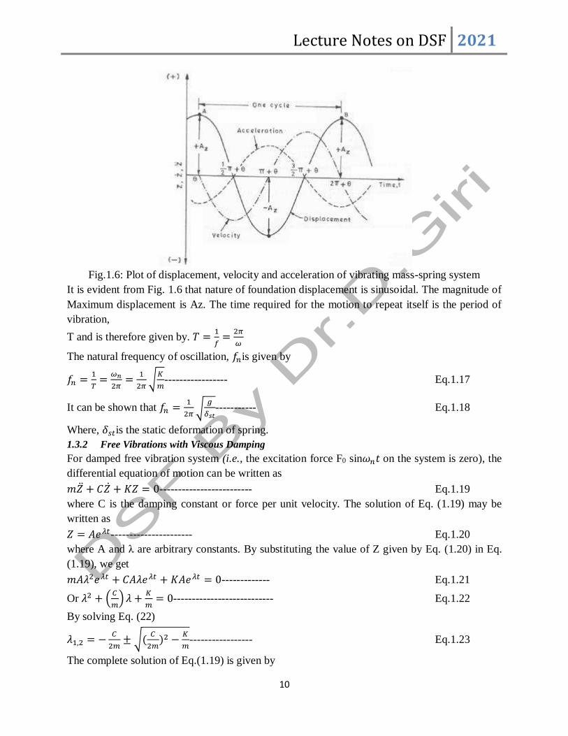
Machines with unbalanced rotating masses develop alternating force as shown in Fig. 1.15 a.
Since horizontal forces on the foundation at any instant cancel, the net vibrating force on the
foundation is vertical and equal to 2𝑚𝑒𝑒𝜔2𝑠𝑖𝑛𝜔𝑡,where me is the mass of each rotating element,
placed at eccentricity e from the centre of rotating shaft and ω is the angular frequency of
masses. Fig. 1.15 b shows such a system mounted on elastic supports with dashpot representing
viscous damping.
(a) Rotating mass type excitation (b) Mass-spring-dash pot system
Fig.1.15: Single degree freedom system with rotating mass type excitation

Lecture Notes on DSF 2021
24
The equation of motion can be written as
𝑚�� + 𝐶�� + 𝐾𝑍 = 2𝑚𝑒𝑒𝜔2𝑠𝑖𝑛𝜔𝑡--------------------- Eq.1.106
Where, m is the mass of foundation including 2me. The solution of Eq. (1.106) may be written as,
𝑍 = 𝐴𝑍sin(𝜔𝑡 + 𝜃)-------------------------- ---------- Eq.1.107
Where
𝐴𝑍 =(2𝑚𝑒𝑒
𝑚⁄ )𝜂2
√(1−𝜔2
𝜔𝑛2)
2
+4𝜉2(𝜔
𝜔𝑛)2
-------------------------------------------- Eq.1.108
𝐹0
𝑘= 2𝑚𝑒𝑒
𝜔2
𝐾= 2𝑚𝑒𝑒
𝜔2
𝑚𝜔𝑛2 = (2𝑚𝑒
𝑒
𝑚)𝜉2---------- Eq.1.109
𝜃 = 𝑡𝑎𝑛−1 (2𝜂𝜉
1−𝜂2)--------------- ---------------------- Eq.1.110
Fig.1.16: Response of a mass rotating system
The Eq. (1.108) can be expressed in non-dimensional form as given below:
𝐴𝑍(2𝑚𝑒𝑒
𝑚⁄ )=
𝜂2
√(1−𝜔2
𝜔𝑛2 )
2+4𝜉2(𝜔
𝜔𝑛)2
---------------------------------- Eq.1.111
Differentiating Eq. (1.111) with respect to η and equating to zero. It can be shown that resonance
will occur at a frequency ratio given by:
𝜂 =1
√1−2𝜉2------------------ ---------------- Eq.1.112
Or 𝜔𝑑 =𝜔𝑛
√1−2𝜉2-------------------------- ------ Eq.1.113
By substituting Eq. (1.113) in Eq. (1.111), we get:

Lecture Notes on DSF 2021
25
𝐴𝑍(2𝑚𝑒𝑒
𝑚⁄ )𝑚𝑎𝑥
=1
2𝜉√1−𝜉2----------------- Eq.1.114
=1
2𝜉For small damping
1.7 VIBRATION ISOLATION
In case a machine is rigidly fastened to the foundation, the force will be transmitted directly to
the foundation and may cause objectionable vibrations. It is desirable to isolate the machine from
the foundation through a suitably designed mounting system in such a way that the transmitted
force is reduced.
For example, the inertial force developed in a reciprocating engine or unbalanced forces
produced in any other rotating machinery should be isolated from the foundation so that the
adjoining structure is not set into heavy vibrations. Another example may be the isolation of
delicate instruments from their supports which may be subjected to certain vibrations. In either
case the effectiveness of isolation may be measured in terms of the force or motion transmitted to
the foundation. The first type is known as force isolation and the second type as motion
isolation.
1.7.1 Force Isolation
Figure 1.17 shows a machine of mass m supported on the foundation by means of an isolator
having an equivalent stiffness K and damping coefficient C. The machine is excited with
unbalanced vertical force of magnitude 2𝑚𝑒𝑒𝜔2𝑠𝑖𝑛𝜔𝑡 .The equation of motion of the machine
can be written as:
𝑚�� + 𝐶�� + 𝐾𝑍 = 2𝑚𝑒𝑒𝜔2𝑠𝑖𝑛𝜔𝑡-------------------- Eq.1.115
The steady state motion of the mass of machine can be worked out as
𝑍 =2𝑚𝑒𝑒𝜔
2
𝐾⁄
√(1−𝜔2
𝜔𝑛2)2
+4𝜉2( 𝜔𝜔𝑛)2sin(𝜔𝑡 − 𝜃)----------------- Eq.1.116
=
2𝑚𝑒𝑒𝜔2
𝐾⁄
√(1−𝜂2)2+4𝜉2(𝜂)2sin(𝜔𝑡 − 𝜃)
Where, 𝜃 = 𝑡𝑎𝑛−1 [2𝜂𝜉
1−𝜂2]-------------- Eq.1.117
The only force which can be applied to the foundation is the spring force KZ and the damping
force, 𝐶��; hence the total force transmitted to the foundation during steady state forced vibration
is
𝐹𝑡 = 𝐾𝑍 + 𝐶��---------------------------- --------------------------------------------Eq.1.118
Now substituting Eq. (1.116) in Eq. (1.118), we get
𝐹𝑡 =2𝑚𝑒𝑒𝜔
2
√(1−𝜂2)2+4𝜉2(𝜂)2sin(𝜔𝑡 − 𝜃) + Cω
2𝑚𝑒𝑒𝜔2
𝐾⁄
√(1−𝜔2
𝜔𝑛2)
2
+4𝜉2(𝜔
𝜔𝑛)2
cos(𝜔𝑡 − 𝜃)---------- Eq.1.119

Lecture Notes on DSF 2021
26
Fig.1.17: Machine isolation foundation system
Equation (1.119) can be written as:
𝐹𝑡 = 2𝑚𝑒𝑒𝜔2 √1+(2𝜂𝜉)2
√(1−𝜂2)2+4𝜉2(𝜂)2sin(𝜔𝑡 − 𝛽)------------------- ------------------------Eq.1.120
Where β is the phase difference between the exciting force and the force transmitted to the
foundation and is given by,
𝛽 = 𝜃 − 𝑡𝑎𝑛−1 [𝐶𝜔
𝐾]--------------------- ---------------------------------------------Eq.1.121
Since the force 2𝑚𝑒𝑒𝜔2 is the force which would be transmitted if springs are infinitely rigid, a
measure of the effectiveness of the isolation mounting system is given by,
𝜇𝑇 =𝐹𝑡
2𝑚𝑒𝑒𝜔2 =
√1+(2𝜂𝜉)2
√(1−𝜂2)2+4𝜉2(𝜂)2--------------- ----------------------------------------Eq.1.122
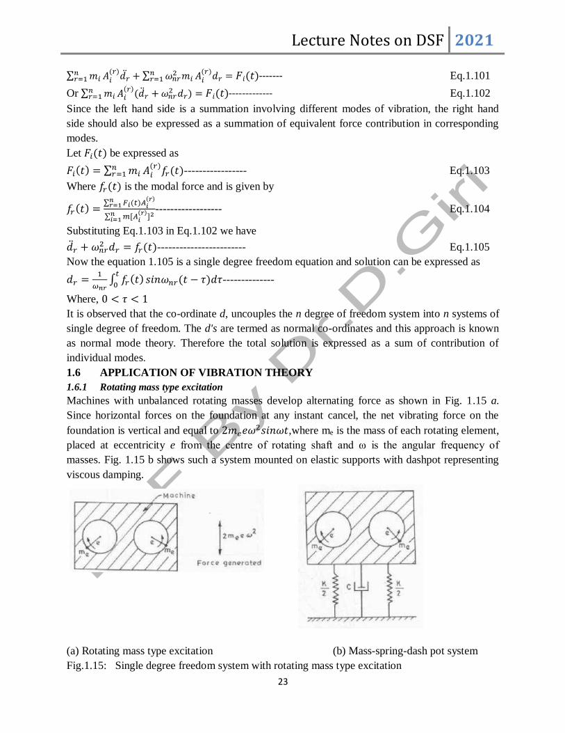
𝜇𝑇 is called the transmissibility of the system.
A plot of 𝜇𝑇 versus η for different values of ξ is shown in Fig.1.18
It will be noted from the figure that for any frequency ratio greater than√2, the force transmitted
to the foundation will be less than the exciting force. However in this case, the presence of
damping reduces the effectiveness of the isolation system as the curves for damped case are
above the undamped ones for η>√2. A certain amount of damping, however, is essential to
maintain stability under transient conditions and to prevent excessive amplitudes when the
vibrations pass through resonance during the starting or stopping of the machine. Therefore, for
the vibration isolation system to be effective η should be greater than√𝟐.
Lecture Notes on DSF 2021
27
Fig.1.18: Transmisibilty versus frequency ratio plot
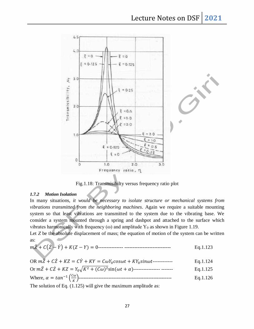
1.7.2 Motion Isolation
In many situations, it would be necessary to isolate structure or mechanical systems from
vibrations transmitted from the neighboring machines. Again we require a suitable mounting
system so that least vibrations are transmitted to the system due to the vibrating base. We
consider a system mounted through a spring and dashpot and attached to the surface which
vibrates harmonically with frequency (ω) and amplitude Y0 as shown in Figure 1.19.
Let Z be the absolute displacement of mass; the equation of motion of the system can be written
as:
𝑚�� + 𝐶(�� − ��) + 𝐾(𝑍 − 𝑌) = 0--------------- ---------------------------- Eq.1.123
OR 𝑚�� + 𝐶�� + 𝐾𝑍 = 𝐶�� + 𝐾𝑌 = 𝐶𝜔𝑌0𝑐𝑜𝑠𝜔𝑡 + 𝐾𝑌0𝑠𝑖𝑛𝜔𝑡------------ Eq.1.124
Or 𝑚�� + 𝐶�� + 𝐾𝑍 = 𝑌0√𝐾2 + (𝐶𝜔)2sin(𝜔𝑡 + 𝛼)---------------- ------- Eq.1.125
Where, 𝛼 = 𝑡𝑎𝑛−1 (𝐶𝜔
𝐾)-------------------------------------------------------- Eq.1.126
The solution of Eq. (1.125) will give the maximum amplitude as:

Lecture Notes on DSF 2021
28
𝑍𝑚𝑎𝑥 = 𝑌0√1+(2𝜂𝜉)2
√(1−𝜂2)2+(2𝜂𝜉)2------------------------------------------------------------- Eq.1.127
The effectiveness of the mounting system (transmissibility) is given by
µ𝑇 =𝑍𝑚𝑎𝑥
𝑌0=
√1+(2𝜂𝜉)2
√(1−𝜂2)2+(2𝜂𝜉)2---------------------------------------------------------- Eq.1.128
Fig.1.19: Motion isolation system
Equation (1.128) is the same expression as Eq. (1.122) obtained earlier. Transmissibility of such
system can also be studied from the response curves shown in Fig.1.18. It is again noted that for
the vibration isolation to be effective, it must be designed in such a way that η>√𝟐.
1.7.3 Materials Used In Vibration Isolation
Materials used for vibration isolation are rubber, felt, cork and metallic springs. The
effectiveness of each depends on the operating conditions.
i) Rubber: Rubber is loaded in compression or in shear; the latter mode gives higher
flexibility. With loading greater than about 0.6 N per sq mm, it undergoes much faster
deterioration. Its damping and stiffness properties vary widely with applied load,
temperature, shape factor, excitation frequency and the amplitude of vibration. The
maximum temperature up to which rubber can be used satisfactorily is about 65°c. It
must not be used in presence of oil which attacks rubber. It is found very suitable for
high frequency vibrations.
ii) Felt: Felt is used in compression only and is capable of taking extremely high loads.
It has very high damping and so is suitable in the range of low frequency ratio. It is
mainly used in conjunction with metallic springs to reduce noise transmission.
Lecture Notes on DSF 2021
29
iii) Cork: Cork is very useful for acoustic isolation and is also used in small pads placed
underneath a large concrete block. For satisfactory working it must be loaded from 10
to 25 N/sq mm. It is not affected by oil products or moderate temperature changes.
However, its properties change with the frequency of excitation.
iv) Metallic springs: Metallic springs are not affected by the operating conditions or the
environments. They are quite consistent in their behaviour and can be accurately
designed for any desired conditions. They have high sound transmissibility which can
be reduced by loading felt in conjunction with it. It has negligible damping and so is
suitable for working in the range of high frequency ratio.
1.8 THEORY OF VIBRATION MEASURING INSTRUMENTS
The purpose of a vibration measuring instrument is to give an output signal which represents, as
closely as possible, the vibration phenomenon. This phenomenon may be displacement, velocity
or acceleration of the vibrating system and accordingly the instrument which reproduces signals
proportional to these are called vibrometers, velometers or accelerometers.
There are essentially two basic systems of vibration measurement. One method is known as the
directly connected system in which motions can be measured from a reference surface which is
fixed. More often such a reference surface is not available. The second system, known as
“Seismic System" does not require a fixed reference surface and therefore is commonly used for
vibration measurement.
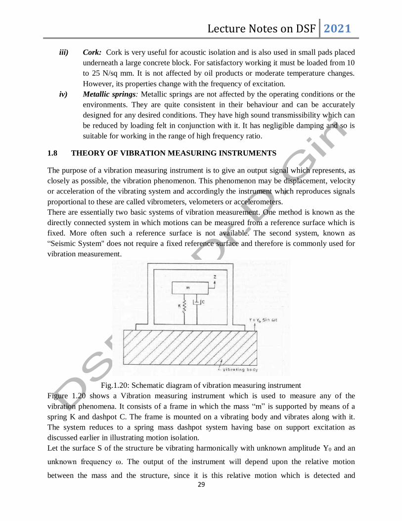
Fig.1.20: Schematic diagram of vibration measuring instrument
Figure 1.20 shows a Vibration measuring instrument which is used to measure any of the
vibration phenomena. It consists of a frame in which the mass “m” is supported by means of a
spring K and dashpot C. The frame is mounted on a vibrating body and vibrates along with it.
The system reduces to a spring mass dashpot system having base on support excitation as
discussed earlier in illustrating motion isolation.
Let the surface S of the structure be vibrating harmonically with unknown amplitude Y0 and an
unknown frequency ω. The output of the instrument will depend upon the relative motion
between the mass and the structure, since it is this relative motion which is detected and
Lecture Notes on DSF 2021
30
amplified. Let Z be the absolute displacement of the mass, then the output of the instrument will
be proportional to X =Z - Y.
The equation of motion of the system can be written as
𝑚�� + 𝐶(�� − ��) + 𝐾(𝑍 − 𝑌) = 0-------------------------- Eq.1.129
Subtracting 𝑚�� from both sides,
𝑚�� + 𝐶�� + 𝐾𝑋 = −𝑚�� = 𝑚𝑌0𝜔2𝑠𝑖𝑛𝜔𝑡----------------- Eq.1.130
The solution can be written as
𝑋 =𝜂2
√(1−𝜂2)2+(2𝜂𝜉)2𝑌0sin(𝜔𝑡 − 𝜃)------------------- ------------------------- Eq.1.131
Where 𝜂 =𝜔
𝜔𝑛= Frequency ratio
𝜉 =damping ratio
𝜃 = 𝑡𝑎𝑛−1(2𝜂𝜉
1−𝜂2)------------------- --------------------------- Eq.1.132
Equation (1.131)can be rewritten as
𝑿 = 𝜼𝟐µ𝒀𝟎𝐬𝐢𝐧(𝝎𝒕 − 𝜽)------------ -------------------------- Eq.1.133
Where
µ =1
√(1−𝜂2)2+(2𝜂𝜉)2--------------------------------------------- Eq.1.134
1.8.1 Displacement Pickup
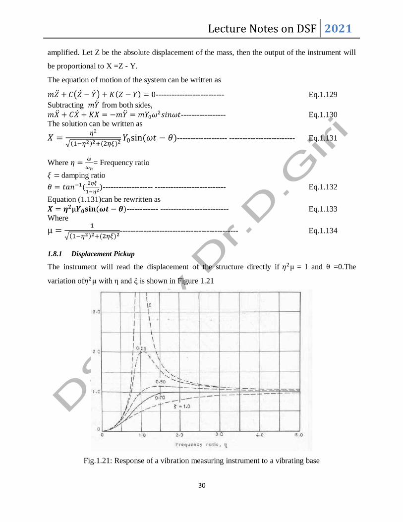
The instrument will read the displacement of the structure directly if 𝜂2µ = I and θ =0.The
variation of𝜂2µ with η and ξ is shown in Figure 1.21
Fig.1.21: Response of a vibration measuring instrument to a vibrating base

Lecture Notes on DSF 2021
31
It is seen when η is large, 𝜂2µ is approximately equal to 1 and θ is approximately equal to 180°.
Therefore to design a displacement pickup, η should be large which means that the natural
frequency of the instrument itself 'should be low compared to the frequency to be measured. Or
in other words, the instrument should have a soft spring and heavy mass. The instrument is
sensitive, flimsy and can be used in a weak vibration environment. The instrument cannot be
used for measurement of strong vibrations.
1.8.2 Acceleration Pickup (Accelerometer)
Equation (1.133) can be rewritten as
�� =1
𝜔𝑛2 µ𝜔
2𝑌0sin(𝜔𝑡 − 𝜃)----------------------------------------- Eq.1.135
The output of the instrument will be proportional to the acceleration of the structure if µ is
constant. It is seen that µ is approximately equal to unity for small values of η. Therefore to
design an acceleration pick up, it should be small which means that the natural frequency of the
instrument itself should be high compared to the frequency to be measured. In other words, the
instrument should have a stiff spring and small mass. The instrument is less sensitive and
suitable for the measurement of strong motion. The instrument size is small.
1.8.3 Velocity Pickup
Equation (1.133) can be rewritten as
�� =1
𝜔𝑛𝜂µ𝑌0𝜔sin(𝜔𝑡 − 𝜃)----------------------------------------- Eq.1.136
The output of the instrument will be proportional to velocity of the structure if 1
𝜔𝑛𝜂µ is a
constant.
At η= 1, Eq. (1.136) can be written as
�� =1
𝜔𝑛
1
2𝜉𝑌0𝜔sin(𝜔𝑡 − 𝜃)-----------------------------------------Eq.1.137 as at η=1,µ =
1
2𝜉
Since 𝜔𝑛 and ξ are constant, the instrument will measure the velocity at η= 1.
It may be noted that the same instrument can be used to measure displacement, acceleration and
velocity in different frequency ranges.
𝑋𝛼𝑌, 𝑖𝑓𝜂 ≫ 1, Displacement pickup (Vibrometer)
𝑋𝛼𝑌, 𝑖𝑓𝜂 ≪ 1, Acceleration pickup (Accelerometers)
𝑋𝛼𝑌, 𝑖𝑓𝜂 = 1, Velocity pickup (Velometers)
Displacement and velocity pickups have the disadvantage of having rather a large size if motions
having small frequency of vibration are to be measured. Calibration of these pickups is not

Lecture Notes on DSF 2021
32
simple. Further corrections have to be made in the observations as the response is not flat in the
starting regions. From the point of view of small size, flat frequency response, sturdiness and
ease of calibration, acceleration pickups are to be favored. They are relatively less sensitive and
this disadvantage can easily be overcome by high gain electronic instrumentation.
1.8.4 Transducer
A transducer is a device for converting the mechanical motion of vibration into an electrical
signal, commonly called pickup.
There are three kinds of transducers: Displacement, Velocity, and Acceleration
1.8.5 Displacement Transducer
It is the most common type of transducer which is operated on the eddy current principle. It sets
up a high-frequency electric field in the gap between the end of the Proximity Probe and the
metal surface that is moving. It senses the change in the gap and measures relative displacement
not absolute displacement.
Proximity Probe
Fig.1.22: Schematic diagram of proximity probe
It is sensitive to shaft surface defects such as scratches, dents and vibrations in conductivity and
permeability.
Senses shaft run out, and it is very difficult to distinguish vibration from run out.
The practical maximum frequency of proximity probes is about 1500Hz.The minimum frequency
is zero. It can also measure static displacement. A useful application of proximity probes is to
measure very slow relative movement like thermal expansion. It is useful in situations where the
vibrating part cannot tolerate the mass of the pickup.

Lecture Notes on DSF 2021
33
1.8.6 Velocity Transducer
Velocity transducer is also called seismic pickup.
The relative motion between the permanent magnet and the coil generates a voltage that is
proportional to the velocity of the motion. The velocity transducer has an internal natural
frequency of about 8 Hz. The velocity transducer is rather large. On small devices this added
mass can significantly affect the vibration output. The coil in the velocity pickup is sensitive to
external electromagnetic fields.
Fig.1.23: Velocity transducer
1.8.7 Acceleration Transducers
Fig.1.24: Accelerator transducer

Lecture Notes on DSF 2021
34
The most common acceleration transducer is the piezoelectric accelerometer It consist of quartz
crystal with a mass bolted on top and a spring compressing the quartz. A property of
piezoelectric material is that it generates an electrical charge output when it is compressed. The
charge output is proportional to force F= ma, force is also proportional to acceleration.
Typically accelerometer has very high natural frequency, typically 25000 Hz Its response is
linear for about 1/3 of this range. It has a useful frequency range of from about 5 to
approximately 100000 Hz depending on its size. The primary considerations in selecting an
accelerometer are sensitivity and frequency response.
If high-amplitude motions are to be measured, i.e. greater than 10g, such as in shock
measurement, then a low-sensitivity accelerometer is appropriate 10 mV/g or less.
If the level motion is to be measured, such as building or structural motions at low frequencies
then a high sensitivity accelerometer should be chosen 1000 mv/g.
For most machinery monitoring,100 mV/g sensitivity accelerometer provide the right balance of
sensitivity and frequency response. Other considerations in accelerometer selection or transducer
are Temperature exposure
Linearity - It is expressed as the percent deviation from a constant value of the sensitivity.
Transverse Sensitivity is the ability of the transducer to detect motion in directions perpendicular
to its sensitive axis.
Damping is very low in piezoelectric accelerometer but can be significant in other types, such as
piezo-resistive accelerometer. Strain sensitivity is the ability of the transducer to generate a
signal when the base is distorted, such as when it is clamped against a non flat surface.

Lecture Notes on DSF 2021
35
2.0 WAVE PROPAGATION; BASIC ELASTIC PROPERTIES AND RELATIONSHIP
2.1 Elastic Constants
An elastic material is one which obeys Hook's law of proportionally between stress and strain.
For an isotropic elastic material subjected to normal stress 𝜎𝑥in the x-direction, the strains in x, y,
z directions are given as
𝑥 =𝜎𝑥
𝐸--------------- Eq.2.1
𝑦 = 𝑧 = −𝜇𝜎𝑥
𝐸---------- Eq.2.2
If the element of the material is subjected to normal stress 𝜎𝑥 , 𝜎𝑦, 𝜎𝑧 ,then by superposition we
obtain
𝑥 =1
𝐸[𝜎𝑥 − 𝜇(𝜎𝑦 + 𝜎𝑧)]-------------- Eq.2.3
𝑦 =1
𝐸[𝜎𝑦 − 𝜇(𝜎𝑥 + 𝜎𝑧)]------------------ Eq.2.4
𝑧 =1
𝐸[𝜎𝑧 − 𝜇(𝜎𝑥 + 𝜎𝑦)]---------------- Eq.2.5
In the above expressions, E is the modulus of elasticity and µ is Poisson's ratio. It may be noted
that here E is dynamic modulus of elasticity.
Equations (3to 5) can be rearranged so, that the stresses are expressed in terms of the strains as
follows: (Timoshenko and Goodier, 1951; Kolsly, 1963).
𝜎𝑥 =𝜇𝐸
(1+𝜇)(1−2𝜇)[ 𝑥 + 𝑦 + 𝑧] +
𝐸
1+𝜇 𝑥----------- Eq.2.6
𝜎𝑦 =𝜇𝐸
(1+𝜇)(1−2𝜇)[ 𝑥 + 𝑦 + 𝑧] +
𝐸
1+𝜇 𝑦----------- Eq.2.7
𝜎𝑧 =𝜇𝐸
(1+𝜇)(1−2𝜇)[ 𝑥 + 𝑦 + 𝑧] +
𝐸
1+𝜇 𝑧----------- Eq.2.8
For simplicity the equations may be written
𝜎𝑥 = 𝜆 + 2𝐺 𝑥---------------------------------------- Eq.2.9
𝜎𝑦 = 𝜆 + 2𝐺 𝑦---------------------------------------- Eq.2.10
𝜎𝑧 = 𝜆 + 2𝐺 𝑧----------------------------------------- Eq.2.11
In which
= 𝑥 + 𝑦 + 𝑧------------------ --------------------- Eq.2.12
𝜆 =µ𝐸
(1+𝜇)(1−2𝜇)------------------------------------------ Eq.2.13
𝐺 =𝐸
2(1+𝜇)------------------------------------------------ Eq.2.14
Similarly in an isotropic elastic material, there exists linear relation between shear stress and
shear strain. Thus
𝛾𝑥𝑦 =𝜏𝑥𝑦
𝐺------------------ ------------------------------- Eq.2.15
𝛾𝑦𝑧 =𝜏𝑦𝑧
𝐺-------------------------------------------------- Eq.2.16
𝛾𝑥𝑧 =𝜏𝑥𝑧
𝐺--------------------------------------------------- Eq.2.17
G is the shear modulus or rigidity modulus and is the same as given by Eqs. (2.9 to 2.11).

Lecture Notes on DSF 2021
36
Equations (2.9 to 2.11) and (2.15 to 2.17) comprise six equations that define the stress-strain
relationship
2.2 WAVE PROPAGATION IN AN INFINITE, HOMOGENEOUS, ISOTROPIC,
ELASTIC MEDIUM
'
In this section, the propagation of stress waves in an infinite, homogeneous, isotropic medium
presented in Figure.2.1 shows the stresses acting on a soil element with sides dx, dy, dz. For
obtaining the differential equations of motion, the sum of the forces acting parallel to each axis is
considered.
In the x-direction the equilibrium equation is given as
Fig. 2.1: Stress on an element of an infinite elastic medium
⌊𝜎𝑥 − (𝜎𝑥 +𝜕𝜎𝑥
𝜕𝑥𝑑𝑥)⌋ (𝑑𝑦. 𝑑𝑧) + ⌊𝜏𝑥𝑧 − (𝜏𝑥𝑧 +
𝜕𝜏𝑥𝑧
𝜕𝑧𝑑𝑧)⌋ (𝑑𝑥. 𝑑𝑦) + ⌊𝜏𝑦𝑥 − (𝜏𝑦𝑥 +
𝜕𝜏𝑦𝑥
𝜕𝑦𝑑𝑦)⌋ (𝑑𝑥. 𝑑𝑧) + 𝜌(𝑑𝑥. 𝑑𝑦. 𝑑𝑧)
𝜕2𝑢
𝜕𝑡2= 0---------------------------- Eq.2.18
Or,
𝜌𝜕2𝑢
𝜕𝑡2=
𝜕𝜎𝑥
𝜕𝑥+
𝜕𝜏𝑥𝑦
𝜕𝑦+
𝜕𝜏𝑥𝑧
𝜕𝑧------------------------------------------------ Eq.2.19 (a)
Equations similar to Eq. (1), it can be written for the y -and z -directions. These will give
𝜌𝜕2𝑣
𝜕𝑡2=
𝜕𝜏𝑦𝑧
𝜕𝑥+
𝜕𝜎𝑦
𝜕𝑦+
𝜕𝜏𝑥𝑧
𝜕𝑧------------------------------------------------- Eq.2.19 (b)
𝜌𝜕2𝜔
𝜕𝑡2=
𝜕𝜏𝑥𝑧
𝜕𝑥+
𝜕𝜏𝑥𝑦
𝜕𝑦+
𝜕𝜎𝑧
𝜕𝑧------------------------------------------------- Eq.2.19 (c)

Lecture Notes on DSF 2021
37
In the above expressions, ρ is the mass density of the soil; u, v and ω are displacements in the x,
y, and z directions respectively. To express the right hand sides of these Eqs., the relationship for
an elastic medium given is used. The equations for strains and rotations of elastic and isotropic
materials in terms of displacements are as follows:
2.2.1 Axial Strains
𝑥 =𝜕𝑢
𝜕𝑥----------------- Eq.2. 20(a)
𝑦 =𝜕𝑣
𝜕𝑦---------------- Eq.2. 20(b)
𝑧 =𝜕𝜔
𝜕𝑧--------------- Eq.2. 20(c)
Shearing Strains:
𝛾𝑥𝑦 =𝜕𝑣
𝜕𝑥+
𝜕𝑢
𝜕𝑦------------ Eq.2. 21(a)
𝛾𝑦𝑧 =𝜕𝜔
𝜕𝑦+
𝜕𝑣
𝜕𝑧---------------- Eq.2 .21(b)
𝛾𝑥𝑧 =𝜕𝜔
𝜕𝑥+
𝜕𝑢
𝜕𝑧-------------------- Eq.2. 21(c)
Rotations:
2𝜔𝑥 =𝜕𝜔
𝜕𝑦−
𝜕𝑣
𝜕𝑧------------ Eq.2. 22(a)
2𝜔𝑦 =𝜕𝑢
𝜕𝑧−
𝜕𝜔
𝜕𝑥------------- Eq.2 .22(b)
2𝜔𝑧 =𝜕𝑣
𝜕𝑥−
𝜕𝑢
𝜕𝑦---------------- Eq.2. 22(c)
2.2.2 Compression Waves
Substitution of Eq.2. 9, 2 .15 and 2.17 in Eq.2. 19 (a) gives
𝜌𝜕2𝑢
𝜕𝑡2=
𝜕
𝜕𝑥(𝜆 + 2𝐺 𝑥) +
𝜕
𝜕𝑦(𝐺𝛾𝑥𝑦) +
𝜕
𝜕𝑧(𝐺𝛾𝑥𝑧)-------------- Eq.2. 23
Or
𝜌𝜕2𝑢
𝜕𝑡2=
𝜕
𝜕𝑥(𝜆 + 2𝐺 𝑥) + 𝐺
𝜕
𝜕𝑦(𝜕𝑣
𝜕𝑥+
𝜕𝑢
𝜕𝑦) + 𝐺
𝜕
𝜕𝑧(𝜕𝑢
𝜕𝑧+
𝜕𝜔
𝜕𝑥)----------- Eq.2. 24
𝜌𝜕2𝑢
𝜕𝑡2=
𝜕
𝜕𝑥(𝜆 + 2𝐺 𝑥) + 𝐺
𝜕
𝜕𝑦(𝜕𝑣
𝜕𝑥+
𝜕𝑢
𝜕𝑦) + 𝐺
𝜕
𝜕𝑧(𝜕𝑢
𝜕𝑧+
𝜕𝜔
𝜕𝑥)----------- Eq.2. 25
𝜌𝜕2𝑢
𝜕𝑡2= 𝜆
𝜕
𝜕𝑥+ 𝐺 ⌈
𝜕2𝑢
𝜕𝑥2+
𝜕2𝑣
𝜕𝑥𝜕𝑦+
𝜕2𝜔
𝜕𝑥𝜕𝑧+
𝜕2𝑢
𝜕𝑥2+
𝜕2𝑢
𝜕𝑦2+
𝜕2𝑢
𝜕𝑧2⌉--------------- Eq.2. 26
As 𝜕2𝑢
𝜕𝑥2+
𝜕2𝑣
𝜕𝑥𝜕𝑦+
𝜕2𝜔
𝜕𝑥𝜕𝑧=
𝜕
𝜕𝑥
The equation Eq.2. 26 can be rewritten as
𝜌𝜕2𝑢
𝜕𝑡2= (𝜆 + 𝐺)
𝜕
𝜕𝑥+ 𝐺∇2𝑢------------------------------------------------- Eq. 2. 27(a)
Where ∇2=𝜕2
𝜕𝑥2+
𝜕2
𝜕𝑦2+
𝜕2
𝜕𝑧2
Similarly corresponding equations in other directions can be written as
𝜌𝜕2𝑣
𝜕𝑡2= (𝜆 + 𝐺)
𝜕
𝜕𝑦+ 𝐺∇2𝑣------------ --------------------------------- Eq.2. 27(b)
𝜌𝜕2𝜔
𝜕𝑡2= (𝜆 + 𝐺)
𝜕
𝜕𝑧+ 𝐺∇2𝜔-------------------------------------------- Eq. 2. 27(c)

Lecture Notes on DSF 2021
38
Equations (2. 27) are the equations of motion of an infinite homogeneous, isotropic, and
elastic medium. On differentiating these equations with respect to x, y and z, respectively, and
adding, we get
𝜌𝜕2
𝜕𝑡2[𝜕𝑢
𝜕𝑥+
𝜕𝑣
𝜕𝑦+
𝜕𝜔
𝜕𝑧] = (𝜆 + 𝐺) [
𝜕2
𝜕𝑥2+
𝜕2
𝜕𝑦2+
𝜕2
𝜕𝑧2] + 𝐺∇2 (
𝜕𝑢
𝜕𝑥+
𝜕𝑣
𝜕𝑦+
𝜕𝜔
𝜕𝑧)------------- Eq.2. 28
𝜌𝜕2
𝜕𝑡2= (𝜆 + 𝐺)(∇2 ) + (𝐺∇2 )----------------------- Eq.2. 29
Hence, 𝜌𝜕2
𝜕𝑡2= (𝜆 + 2𝐺)(∇2 )--------------- Eq.2. 30
0r
𝜕2
𝜕𝑡2=
(𝜆+2𝐺)
𝜌(∇2 ) = 𝑉𝑝
2∇2 ------------------ Eq.2. 31
Where 𝑉𝑝2 =
(𝜆+2𝐺)
𝜌----------------------------- Eq.2.32
Vp is the ve1ocity of compression waves which is also referred as primary wave or, P-wave. It is
important to note the difference in the wave velocities for an infinite elastic medium with those
obtained for an elastic rod is, 𝑉𝑐 = √𝐸 𝜌⁄ : but in the infinite medium, 𝑉𝑝 = √(𝜆+2𝐺)
𝜌. This means
that Vp >Vc, that is compression wave travels faster in infinite medium. It is due to the fact that
in infinite medium, there are no lateral displacements, while in the elastic rod lateral
displacements are possible.
2.2.3 Shear-Waves
Differentiating Eq. (2.27,b) with respect to z and Eq. (2.27,c) with respect to y, we get
𝜌𝜕2
𝜕𝑡2(𝜕𝑣
𝜕𝑧) = (𝜆 + 𝐺)
𝜕
(𝜕𝑦)(𝜕𝑧)+ 𝐺∇2
𝜕𝑣
𝜕𝑧----------------- Eq. 2.33
𝜌𝜕2
𝜕𝑡2(𝜕𝜔
𝜕𝑦) = (𝜆 + 𝐺)
𝜕
(𝜕𝑦)(𝜕𝑧)+ 𝐺∇2
𝜕𝜔
𝜕𝑦--------------- Eq.2.34
Subtracting Eq.2.34 from Eq.2.33, we get
𝜌𝜕2
𝜕𝑡2(𝜕𝜔
𝜕𝑦−
𝜕𝑣
𝜕𝑧) = 𝐺∇2 (
𝜕𝜔
𝜕𝑦−
𝜕𝑣
𝜕𝑧)----------------------- Eq.2.35
FromEq.(2.22,a)
2𝜔𝑥 =𝜕𝜔
𝜕𝑦−𝜕𝑣
𝜕𝑧
Therefore,
𝜌𝜕2𝜔𝑥
𝜕𝑡2= 𝐺∇2𝜔𝑥 --------------------- Eq.2.35
Or,
𝜕2𝜔𝑥
𝜕𝑡2=
𝐺
𝜌∇2𝜔𝑥 = 𝑉𝑠
2∇2𝜔𝑥 --------------------- Eq.2.36 (a)
Similar expression can be obtained for ��𝑦 𝑎𝑛𝑑𝜔𝑧 as
𝜕2𝜔𝑦
𝜕𝑡2=
𝐺
𝜌∇2𝜔𝑦 = 𝑉𝑠
2∇2𝜔𝑦 ---------------------- Eq.2. 36 (b)
𝜕2𝜔𝑧
𝜕𝑡2=
𝐺
𝜌∇2𝜔𝑧 = 𝑉𝑠
2∇2𝜔𝑧 --------------------- Eq.2. 36 (c)
The above expressions indicate that the Rotation is propagated with velocity Vs which is equal to

Lecture Notes on DSF 2021
39
√𝐺 𝜌⁄ . Shear wave is also referred as distortion wave or S-wave. It may be noted that shear wave
propagates at the same velocity in both the rigid elastic medium like rod or bar and the infinite-
medium.
2.3 WAVEPROP AGATION IN ELASTIC HALF-SPACE
In an elastically homogeneous ground, stressed suddenly at a point 'S' near its surface as shown
in (Figure 2.2), three elastic waves travel outwards at different speeds. Two are body waves;
which are propagated as spherical, fronts affected only a minor extent by the free surface of the
ground, and the third is a surface wave which is confined to the region, near the free surface.
Fig.2.2: Pulse fronts of the P, S and R waves
The stresses in the P wave, which is a longitudinal wave like a sound wave in air, are thus due to
uniaxial compression, while during the passage of an S wave the medium is subjected to shear
stress. The surface wave travels more slowly than either body wave, and is generally complex.
This wave was first studied by Rayleigh (1885) and later was, described in detail by Lamb
(1904). It is referred as Rayleigh wave or R-wave. The influence of Raleigh wave decreases
rapidly with depth.
The half space is defined as the x-y plane with z assumed to be positive toward the interior of the
half-space as shown in Figure 2.3. Let u and w represent the displacements in the directions x
and z, respectively and are independent of y, then
𝑢 =𝜕∅
𝜕𝑥+
𝜕𝜑
𝜕𝑧-------------------------------------------------------------------Eq.2.37
𝜔 =𝜕∅
𝜕𝑧−
𝜕𝜑
𝜕𝑥------------------------------------------------------------------ Eq.2.38
Where ∅and φ are two potential function. As 𝜕𝑣
𝜕𝑦=0, the dilation of the wave can be written as
=𝜕𝑢
𝜕𝑥+
𝜕𝜔
𝜕𝑧= [
𝜕2∅
𝜕𝑥2+
𝜕2𝜑
𝜕𝑥𝜕𝑧] + [
𝜕2∅
𝜕𝑧2−
𝜕2𝜑
𝜕𝑥𝜕𝑧]------------------------------- Eq.2.38
Or, =𝜕2∅
𝜕𝑥2+
𝜕2∅
𝜕𝑧2= ∇2∅----------------------------------------------------- Eq.2.39
Similarly the rotation in x-z plane is given by
2𝜔𝑦 =𝜕𝑢
𝜕𝑧−
𝜕𝜔
𝜕𝑥=
𝜕2𝜑
𝜕𝑥2+
𝜕2𝜑
𝜕𝑧2= ∇2𝜑-----------------------------------------Eq.2.40

Lecture Notes on DSF 2021
40
Fig.2.3: Wave propagation in Elastic half space
𝑢 =𝜕∅
𝜕𝑥+
𝜕𝜑
𝜕𝑧------------------------------------------------------------------- Eq.2.41
𝜔 =𝜕∅
𝜕𝑧−
𝜕𝜑
𝜕𝑥------------------------------------------------------------------ Eq.2.42
Where ∅and φ are two potential function. As 𝜕𝑣
𝜕𝑦=0, the dilation of the wave can be written as
=𝜕𝑢
𝜕𝑥+
𝜕𝜔
𝜕𝑧= [
𝜕2∅
𝜕𝑥2+
𝜕2𝜑
𝜕𝑥𝜕𝑧] + [
𝜕2∅
𝜕𝑧2−
𝜕2𝜑
𝜕𝑥𝜕𝑧]------------------------------- Eq.2.43
Or, =𝜕2∅
𝜕𝑥2+
𝜕2∅
𝜕𝑧2= ∇2∅----------------------------------------------------- Eq.2.44
Similarly the rotation in x-z plane is given by
2𝜔𝑦 =𝜕𝑢
𝜕𝑧−
𝜕𝜔
𝜕𝑥=
𝜕2𝜑
𝜕𝑥2+
𝜕2𝜑
𝜕𝑧2= ∇2𝜑----------------------------------------- Eq.2.45
Substituting u and w from Eq.1 and 2 in, we get
𝜌𝜕
𝜕𝑥(𝜕2∅
𝜕𝑡2) + 𝜌
𝜕
𝜕𝑧(𝜕2𝜑
𝜕𝑡2) = (𝜆 + 2𝐺)
𝜕
𝜕𝑥(∇2∅) + 𝐺
𝜕
𝜕𝑧(∇2𝜑)------------- Eq.2.46
And 𝜌𝜕
𝜕𝑧(𝜕2∅
𝜕𝑡2) − 𝜌
𝜕
𝜕𝑥(𝜕2𝜑
𝜕𝑡2) = (𝜆 + 2𝐺)
𝜕
𝜕𝑧(∇2∅) − 𝐺
𝜕
𝜕𝑥(∇2𝜑)-------- Eq.2.47
The above Eqs (2.46 and2.47) are satisfied if
𝜕2∅
𝜕𝑡2=
(𝜆+2𝐺)
𝜌∇2∅ = 𝑉𝑝
2∇2∅---------------------------------------------------- Eq.2.48
And 𝜕2𝜑
𝜕𝑡2=
𝐺
𝜌∇2𝜑 = 𝑉𝑠
2∇2𝜑---------------------------------------------------- Eq.2.49
Now, consider a sinusoidal wave traveling in the positive x direction. Let the solution of ∅ and 𝜑
be expressed as
∅ = 𝐹(𝑧) exp[𝑖(𝜔𝑡 − 𝑓𝑥)]---------------------- Eq.2.50
And
𝜑 = 𝐺(𝑧) exp[𝑖(𝜔𝑡 − 𝑓𝑥)]----------------------- Eq.2.51
Where F(z) and G(z) are function of depth
And 𝑓 =2𝜋
𝑤𝑎𝑣𝑒𝑙𝑒𝑛𝑔𝑡ℎ
Now substituting Eq. 2.50 into Eq. 2.48 , we get

Lecture Notes on DSF 2021
41
(𝜕2
𝜕𝑡2) {𝐹(𝑧) exp[𝑖(𝜔𝑡 − 𝑓𝑥)]}=𝑉𝑝
2∇2{𝐹(𝑧) exp[𝑖(𝜔𝑡 − 𝑓𝑥)]}---------- Eq.2.52
Or −𝜔2𝐹(𝑧) = 𝑉𝑝2[𝐹"(𝑧) − 𝑓2𝐹(𝑧)]--------------------------------------- Eq.2.53
Where F(z) and G(z) are functions of depth
Similarly, substituting Eq. (2.51) into Eq. (2.49) results in
−𝜔2𝐺(𝑧) = 𝑉𝑠2[𝐺"(𝑧) − 𝑓2𝐺(𝑧)]---------------- Eq.2.54
Where
𝐹"(𝑧) =𝜕2𝐹(𝑧)
𝜕𝑧2---------------------------------------- Eq.2.55
and
𝐺"(𝑧) =𝜕2𝐺(𝑧)
𝜕𝑧2------------------------------------------------- Eq.2.56
Now Equations (2.53) and (2.54) can be rearranged to the form
𝐹"(𝑧) − 𝑞2𝐹(𝑧) = 0-------------------------------- Eq.2.57
𝐺"(𝑧) − 𝑠2𝐹(𝑧) = 0--------------------------------- Eq.2.58
Where
𝑞2 = 𝑓2 −𝜔2
𝑉𝑝2----------------------------------------------- Eq.2.59
𝑠2 = 𝑓2 −𝜔2
𝑉𝑠2------------------- Eq.2.60
Solutions to Eqs. (2.57) and (2.48) can be given as
𝐹(𝑧) = 𝐴1𝑒−𝑞𝑧 + 𝐴2𝑒
𝑞𝑧--------------- Eq.2.61
𝐺(𝑧) = 𝐵1𝑒−𝑠𝑧 + 𝐵2𝑒
𝑠𝑧---------------- Eq.2.62
where A1, A2, B1, and B2 are constants.
It can be seen from Eqs. (2.61) and (2.62) that A2 and B2 must equal zero; otherwise F(z) and
G(z) will approach infinity with depth, which is not the type of wave that is considered here.
With A2 and B2 equal zero, we have
𝐹(𝑧) = 𝐴1𝑒−𝑞𝑧--------------- Eq.2.63
𝐺(𝑧) = 𝐵1𝑒−𝑠𝑧---------------- Eq.2.64
Now combining Eqs. (2.50) and (2.63) and Eqs. (2.51) and (2.64), we get
∅ = (𝐴1𝑒−𝑞𝑧)[exp 𝑖(𝜔𝑡 − 𝑓𝑥)]---------------------- Eq.2.65
𝜑 = (𝐵1𝑒−𝑠𝑧)[𝑒𝑥𝑝𝑖(𝜔𝑡 − 𝑓𝑥)]------------------------ Eq.2.66
The boundary conditions for the two preceding equations are at z = 0, σz = 0, τzx = 0, and τzy = 0.
We have
𝜎𝑧(𝑧=0) = 𝜆 + 2𝐺 𝑧 = 𝜆 + 2𝐺 (𝜕𝜔
𝜕𝑧) = 0------------- Eq.2.67
Combining Eqs. (2.42), (2.444), and (2.65)–(2.67), one obtains
𝐴1[(𝜆 + 2𝐺)𝑞2 − 𝜆𝑓2] − 2𝑖𝐵1𝐺𝑓𝑠 = 0----------- Eq.2.68

Lecture Notes on DSF 2021
42
And 𝐴1
𝐵1=
2𝑖𝐺𝑓𝑠
(𝜆+2𝐺)𝑞2−𝜆𝑓2----------------- Eq.2.69
Similarly, 𝜏𝑧𝑥(𝑧=0) = 𝐺𝛾𝑧𝑥 = 𝐺 (𝜕𝜔
𝜕𝑥+
𝜕𝑢
𝜕𝑧) = 0----- Eq.2.70
Again, combining Eqs. (2.21), (2.23), (2.65), (2.66), and (2.70),
2𝑖𝐴1𝑓𝑞 + (𝑠2 + 𝑓2)𝐵1 = 0------------- Eq.2.71
OR 𝐴1
𝐵1=
(𝑠2+𝑓2)
2𝑖𝑓𝑞--------------- Eq.2.72
Equating the right-hand sides of Eqs.( 2.69) and (2.72),
2𝑖𝐺𝑓𝑠
(𝜆+2𝐺)𝑞2−𝜆𝑓2=
(𝑠2+𝑓2)
2𝑖𝑓𝑞-------------- Eq.2.73
4𝐺𝑓2𝑠𝑞 = (𝑠2 +𝑓2) [(𝜆 + 2𝐺)𝑞2 − 𝜆𝑓2]------- Eq.2.74
Or, 16𝐺2𝑓4𝑠2𝑞2 = (𝑠2 + 𝑓2)2[(𝜆 + 2𝐺)𝑞2 − 𝜆𝑓2]----------Eq.2.75
Substituting for q and s and then dividing both sides of Eq. (2.75) by G2f8, we get
16 (1 −𝜔2
𝑉𝑝2𝑓2
) (1 −𝜔2
𝑉𝑠2𝑓2
) = [2 − (𝜆+2𝐺
𝐺)
𝜔2
𝑉𝑝2𝑓2
]2
[2 −𝜔2
𝑉𝑠2𝑓2
]2
---------------------- Eq.2.76
However,𝑤𝑎𝑣𝑒𝑙𝑒𝑛𝑔𝑡ℎ =𝑣𝑒𝑙𝑜𝑐𝑖𝑡𝑦𝑜𝑓𝑤𝑎𝑣𝑒
𝜔2𝜋⁄
𝑓 =𝜔
𝑉𝑟----------------- Eq.2.77
So, 𝜔2
𝑉𝑝2𝑓2
=𝜔2
𝑉𝑝2(𝜔
2
𝑉𝑟2⁄ )=
𝑉𝑟2
𝑉𝑝2=𝛼
2𝑉2---------------- Eq.2.78
Similarly, 𝜔2
𝑉𝑠2𝑓2
=𝜔2
𝑉𝑠2(𝜔
2
𝑉𝑟2⁄ )=
𝑉𝑟2
𝑉𝑠2=𝑉
2----------------- Eq.2.79
Where 𝛼2 =𝑉𝑠2
𝑉𝑝2
However, 𝑉𝑝2 = 𝜆 + 2𝐺
𝜌⁄ and 𝑉𝑠2 = 𝐺
𝜌⁄
So, 𝛼2 =𝑉𝑠2
𝑉𝑝2 =
𝐺
𝜆+2𝐺------------------ Eq.2.80
The term 𝛼2 can also be expressed in terms of Poisson’s ratio. From the relations given in Eq.
(2.81),
2𝜇𝐺
1−2𝜇---------------------- Eq.2.81
Substitution of this relation in Eq. (2.80) yields,
𝛼2 =𝐺
𝜆+2𝐺=
(1−2𝜇)
2(1−𝜇)--------------- Eq.2.82
Again, substituting Eqs. (2.78), (2.79), and (2.80) into Eq. (2.76),
16(1 − 𝛼2𝑉2)(1 − 𝑉2) = (2 − 𝑉2)(2 − 𝑉2)2
Or, 𝑉6 − 8𝑉4 − (16𝛼2 − 24)𝑉2 − 16(1 − 𝛼2) = 0------------- Eq.2.83

Lecture Notes on DSF 2021
43
Equation (2.83) is a cubic equation in V2. For a given value of Poisson’s ratio, the proper value
of V2 can be found and, hence, so can the value of Vr in terms of Vp or Vs.
Example 1:
Given μ = 0.25, determined the value of the Rayleigh wave velocity in terms of Vs
Solution:
𝑉6 − 8𝑉4 − (16𝛼2 − 24)𝑉2 − 16(1− 𝛼2) = 0
For µ=0.25
𝛼2 =1 − 2𝜇
2 − 2𝜇= 1/3
𝑉6 − 8𝑉4 − (16 ×1
3− 24)𝑉2 − 16(1 −
1
3) = 0
3𝑉6 − 24𝑉4 + 56𝑉2 − 32 = 0
(𝑉2 − 4)(3𝑉4 − 12𝑉2 + 8) = 0
Therefore, 𝑉2 = 4, 2 +2
√3, 2 −
2
√3
If V2=4, 𝑆2
𝑓2= 1 − 𝑉2 = 1 − 4 = −3
So S/f is imaginary. This is also the case for V2=2 +2
√3
It can be seen that when q/f and s/f are imaginary, it does not yield the primary and secondary
waves as discussed.
For V2=2 −2
√3, 𝑣 =
𝑣𝑟
𝑣𝑠=0.9194
Or 𝑣𝑟=0.9194𝑣𝑠

Lecture Notes on DSF 2021
44
3.0 LIQUEFACTION OF SOIL
Previous earthquake devastation was an illustration of catastrophic damages to structures and
resulting in loss of life which was due to liquefaction phenomenon. Liquefaction is defined as a
condition where a soil will undergo continuation of deformation at a constant low residual stress
or with no residual resistance, due to the build-up and maintenance of high pore water pressure
which reduces the effective confining pressure to a very low value. The pore pressure so build-up
leading to true liquefaction of this type may be due either to static or cyclic stress applications.
3.1 Initial Liquefaction
It denotes a condition where, during the course of cyclic stress applications, the residual pore water
pressure on completion of any full stress -cycle becomes equal to the applied confining stress.
MECHANISM OF LIQUEFACTION:
The strength of sand is primarily due to internal friction. In saturated state it may be expressed as
𝑠 = 𝜎𝑛 tanφ------ Eq.3.1
Where S= Shear strength of sand
𝜎𝑛 = Effective normal stress on any plane at a depth of z
Φ= Angle of internal friction
Fig.3.1. Section of ground showing the position of water table
When a saturated sand is subjected to ground vibrations, it tends to compact and decrease
volume, if drainage is restrained the tendency to decrease in volume results in an increase in pore
pressure.
The strength may now be expressed as,
𝑆𝑑𝑦𝑛 = (𝜎𝑛 − 𝑢𝑑𝑦𝑛)𝑡𝑎𝑛∅𝑑𝑦𝑛------------- Eq.3.2
𝑆𝑑𝑦𝑛=Shear strength of soil under vibration
𝑢𝑑𝑦𝑛=Excess pore water due to ground vibration
∅𝑑𝑦𝑛=angle of internal of friction under vibration
It is observed that with development of additional positive pore pressure, the strength of sand is
reduced.
For complete loss of strength, shear strength becomes zero, 𝑆𝑑𝑦𝑛=0
Thus, 𝜎𝑛 − 𝑢𝑑𝑦𝑛=0

Lecture Notes on DSF 2021
45
Or 𝜎𝑛 =𝑢𝑑𝑦𝑛, hence 𝑢𝑑𝑦𝑛
𝜎𝑛 =1--------- Eq.3.3
Now 𝑢𝑑𝑦𝑛can be expressed in terms of rise in water head and be written as
𝛾𝑤ℎ𝑤𝐺−1
1+𝑒𝛾𝑤𝑍
=1---- Eq.3.4
Or ℎ𝑤
𝑍=
𝐺−1
1+𝑒--------- Eq.3.5
This is the critical hydraulic gradient.
It is seen that, because of increase in pore water pressure the effective stress reduces, resulting in
loss of strength. Transfer of inter granular stress takes place from soil grains to pore water. Thus
if this transfer is completed, there is complete loss of strength, resulting in what is known as
complete liquefaction. However, if only partial transfer of stress from the grains to the pore
water occurs, there is partial loss of strength resulting in partial liquefaction. In case of complete
liquefaction, the effective stress is lost and the sand-water mixture behaves as a viscous material
and process of consolidation starts. Due to surface settlement, resulting in closer packing of sand
grains occurs. Thus the structures resting on such a material start sinking. The rate of sinking of
structures depends upon the time for which the sand remains in liquefied state. Liquefaction of
sand may develop at any zone of a deposit, where the necessary combination of in-situ density,
surcharge conditions and vibration characteristics occur. Such a zone may be at the surface or at
some depth below the ground surface, depending only on the state of sand and the induced
motion.
3.3 FACTORS AFFECTING LIQUEFACTION
The factors affecting liquefaction are summarised below
a) Soil Type: Liquefaction occurs in cohesion-less soils as they lose their strength
completely under vibration due to the development of pore pressures which in turn
reduce the effective stress to zero. Liquefaction does not occur in case of cohesive soils.
Only highly sensitive clays may lose their strength substantially under vibration.
b) Grain Size and Its Distribution: Fine and uniform sands are more prone to liquefaction
than coarser ones. Since the permeability of coarse sand is greater than fine sand, the pore
pressure developed during vibrations can dissipate faster.
c) Initial Relative Density: It is one of the most important factors controlling liquefaction.
Both pore pressures and settlement are considerably reduced during vibrations with
increase in initial relative density and hence chances of liquefaction and excessive
settlement reduce with increased relative density.
d) Vibration Characteristics: Out of the four parameters of dynamic load namely (i)
frequency; (ii) amplitude; (iii) acceleration; and (iv) velocity; frequency and acceleration
are more important. Frequency .of the dynamic load plays vital role, only if it is close to
the natural frequency of the system. Further the liquefaction depends on the type of the
dynamic load i.e. whether it is a transient load or the load that causes steady vibration.
For a given acceleration, liquefaction occurs only after a certain number of cycles

Lecture Notes on DSF 2021
46
imparted to the deposit. Further, horizontal vibrations have more severe effect than
vertical vibrations. Multi directional shaking is more severe than one directional loading
(Seed at al.1977), as the pore water pressure build up is much faster and the stress ratio
required is about 10 percent less than that required for unidirectional shaking.
e) Location of Drainage and Dimension of Deposit: Sands are more pervious than fine
grained soil. However, if a pervious deposit has large dimensions, the drainage path
increases and the deposit may behave as un-drained, thereby, increasing the chances of
liquefaction of such a deposit. The drainage path is reduced by the introduction of drains
made out of highly pervious material.
f) Surcharge Load: If the surcharge load, i.e. the initial effective stress is large, then
transfer of stress from soil grains to pore water will require higher intensity vibrations or
vibration for a longer duration. If the initial stress condition is not isotropic as in field,
then stress condition causing liquefaction depends upon K0 (coefficient of earth pressure
at rest) and for K0> 5, the stress condition required to cause liquefaction increases by at
least 50%.
g) Method of Soil Formation: Sands unlike clays do not exhibit a characteristics structure.
But recent investigations show that liquefaction characteristics of saturated sands under
cyclic loading are significantly influenced by method of sample preparation and by soil
structure.
h) Period under Sustained Load: Age of sand deposit may influence liquefaction
characteristics. A 75% increase in liquefaction resistance has been reported on
liquefaction of undisturbed sand compared to its freshly prepared sample which may be
due to some form of cementation or welding at contact points of sand particles and
associated with secondary compression of soil.
i) Previous Strain History: Studies on liquefaction characteristics of freshly deposited
sand and of similar deposit previously subjected to some strain history reveal, that
although the prior strain history caused no significant change in the density of the sand, it
increased the stress that causes liquefaction by a factor of 1.5.
j) Trapped Air: If air is trapped in saturated soil and pore pressure develop, a part of it is
dissipated due to the compression of air, hence trapped air helps to reduce the possibility
of liquefaction.
k) Groundwater Table: The most conducive condition to liquefaction is near the surface of
ground water table. Unsaturated soil located above the groundwater table will not liquefy.
At the location where groundwater table significantly fluctuates, the liquefaction will also
fluctuate.
3.4 EVALUATION OF ZONE OF LIQUEFACTION IN FIELD
At a depth below the ground surface, liquefaction will occur if shear stress induced by
earthquake is more than the shear stress predicted. By comparing the induced and predicted shear
stresses at various depths, liquefaction zone can be obtained.

Lecture Notes on DSF 2021
47
In a sand deposit consider a column of soil of height h and unit area of cross section subjected to
maximum ground acceleration Qmax(Fig.3.2).
Fig.3.2: Maximum shear stress at a depth for a rigid soil column
Assuming the soil column to behave as a rigid body, the inertia force F can be obtained as
𝐹 =𝑊
𝑔𝑎𝑚𝑎𝑥--------- Eq.3.6
Or =𝛾𝑧
𝑔𝑎𝑚𝑎𝑥 = 𝜎0
𝑎𝑚𝑎𝑥
𝑔-------------- Eq.3.7
The maximum shear stress 𝜏𝑚𝑎𝑥 at a depth h is given by
𝜏𝑚𝑎𝑥 =𝐹
𝐴=𝜎0
𝑎𝑚𝑎𝑥
𝑔----------------- Eq.3.8
As base area of soil column is taken as unity
Where g = Acceleration due to gravity and γ = Unit weight of soil
Since the soil column behaves as a deformable body, the actual shear stress at depth h, (𝜏𝑚𝑎𝑥) is
taken as
𝜏𝑎𝑐𝑡 = 𝑟𝑑𝜏𝑚𝑎𝑥 = 𝑟𝑑(𝛾ℎ
𝑔)𝑎𝑚𝑎𝑥------ Eq.3.9
Where 𝑟𝑑= Depth reduction factor
If linear variation is assumed between reduction factor and depth, than rd can be taken as
𝑟𝑑 = 1 − 0.012𝑧------- Eq.3.10
The above relation is valid for depth up to 15 m.
According to Seed and Idriss (1971), the average equivalent uniform shear stress 𝜏𝑎𝑣𝑔 is about
65 percent of the maximum shear stress 𝜏𝑚𝑎𝑥 .Therefore
𝜏𝑎𝑣𝑔 = 0.65𝛾𝑧
𝑔𝑎𝑚𝑎𝑥𝑟𝑑-------- Eq.3.11
The corresponding number of significant cycles Ns for 𝜏𝑎𝑣𝑔 is given in table Table.3.1
Table 3.1: Significant cycles Ns corresponding to 𝜏𝑎𝑣𝑔
Earthquake magnitude, M on Richter’s scale Ns
7 10
7.5 20
8.0 30

Lecture Notes on DSF 2021
48
In order to felicitate liquefaction analysis one non dimensional parameter known as Cyclic Stress
Ratio (CSR) or Seismic Stress Ratio (SSR), can be defined as
𝐶𝑆𝑅𝑜𝑟𝑆𝑆𝑅 =𝜏𝑎𝑣𝑔
𝜎0′ ---------- Eq.3.12
Thus, 𝐶𝑆𝑅𝑜𝑟𝑆𝑆𝑅 = 0.65𝑟𝑑(𝜎0
𝜎0′)
𝑎𝑚𝑎𝑥
𝑔------ Eq.3.13
Seed and Idriss (1971) suggested the value of cyclic stress ratio values Cr as given in Table 3.2
Table 3.2: Values of Cr corresponding to Relative density
Relative density DR (%) Cr
0-50 0.57
60 0.60
80 0.68
It was observed that up to a relative density of 80%, the peak pulsating shear stress causing
liquefaction increases almost linearly with the increase in relative density. Keeping this fact in
view, the following general relation is suggested:
(𝜏ℎ
𝜎𝑣)𝑓𝑖𝑒𝑙𝑑𝐷𝑅 = (
𝜎𝑑
2𝜎3)𝑡𝑟𝑖𝑎𝑥,50𝐶𝑟
𝐷𝑅
50---------- Eq.3.14
Where, (𝜏ℎ
𝜎𝑣)𝑓𝑖𝑒𝑙𝑑𝐷𝑅= Cyclic shear stress ratio in field at relative density of DR percentage
(𝜎𝑑
2𝜎3)𝑡𝑟𝑖𝑎𝑥,50=Stress ratio obtained from triaxial test at relative density of 50%. It can be
determined from Fig.3.3
Fig. 3.3: Stress condition causing liquefaction of sands (Seed and Idriss, 1971)
3.5 THE PROCEDURE OF LOCATING LIQUEFACTION ZONE CAN BE SUMMARISED
IN FOLLOWING STEPS
i) Establish the design earthquake, and obtain peak ground acceleration amax. Also obtain
number of significant cycles Ns corresponding to earthquake magnitude using Table.2
Lecture Notes on DSF 2021
49
ii) Using Eq. 11 determine 𝜏𝑎𝑣𝑔 at depth h below ground surface.
iii) Using Fig.2, determine the value of 𝜎𝑑
2𝜎3for given value of D50 of soil and number of
equivalent cycles NS for the relative density of 50%.
iv) Using Eq. 12, determine the value of (𝜏ℎ
𝜎𝑣)𝑓𝑖𝑒𝑙𝑑𝐷𝑅 for the relative density of DR of the
soil at site. Multiplying (𝜏ℎ
𝜎𝑣)𝑓𝑖𝑒𝑙𝑑𝐷𝑅 with effectives stress at depth h, we can obtain
the value of shear stress 𝜏ℎ required for causing liquefaction.
v) At depth h, liquefaction will occur if 𝜏𝑎𝑣𝑔 > 𝜏ℎ
vi) Repeat steps (ii) to (iv) for other values of h to locate the zone of liquefaction.
𝜏𝑎𝑣𝑔 and 𝜏ℎ can be plotted in a graph to identify the zone of liquefaction.
Problem No.1
At a given site, a boring supplemented with standard penetration tests was done up to 15.0m
depth. The results of the boring are as given below:
Depth
(m)
Classification of soil D50
(mm)
N-Value DR
(%)
Remarks
1.5 SP 0.18 3 19 Position of ground water
lies 1.5 m below the ground
surface
3.0 SP 0.2 5 30
4.5 SM 0.12 6 35
6.0 SM 0.14 9 40
7.5 SM 0.13 12 45 𝛾𝑚𝑜𝑖𝑠𝑡=19 kN/m3
𝛾𝑠𝑢𝑏=10 kN/m3
9.0 SP 0.16 17 52
10.5 SW 0.2 20 52
12.0 SW 0.22 18 46
13.0 SW 0.22 24 60
15.0 SW 0.24 30 65
The site is located in seismically, active region, and is likely to be subjected by an earthquake of
Magnitude 7.5. Determine the zone of liquefaction using Seed and ldriss (1971) method.
3.6 EVALUATION OF LIQUEFACTION POTENTIAL USING STANDARD
PENETRATION RESIST ANCE
The standard penetration test is most commonly used in-situ test in a bore hole to have fairly
good estimation of relative density of cohesion-less soil. Since liquefaction primarily depends on
the initial relative density of saturated sand, many researchers have made attempt to develop
correlations in liquefaction potential and standard penetration resistance. IS: 2131-1981 gives the
standard procedure to carry out standard penetration test. SPT values (N) obtained in the field for
sand have to be corrected for accounting the effect of over burden pressure as below:
𝑁𝑐𝑜𝑟𝑟𝑒𝑐𝑡𝑒𝑑 = 𝐶𝑁𝑁𝑓𝑖𝑒𝑙𝑑------------ Eq.3.15
CN = Correction factor obtained from Figure 3.4 or it can be also be found from the expression
𝐶𝑁 = √100
��------ Eq.3.16
�� is the effective stress in kN/m2

Lecture Notes on DSF 2021
50
Fig. 3.4: Chart for correction of N value for over burden pressure
3.7 FOLLOWING PROCEDURE FOR LIQUEFACTION ANALYSIS IS USED
i) Establish the design earthquake, and obtain the peak ground acceleration amax. Also
obtain number of significant cycles corresponding to the magnitude of earthquake
using Table 3.1.
ii) Using Eq. 3.11 determine 𝜏𝑎𝑣𝑔 at depth h below ground surface.
iii) Determine the value of standard penetration resistance value (N) at depth h below
ground surface. Obtain corrected Ncorrected value after applying overburden correction
to N using Fig.3.4
iv) Using Fig.3.3, determine 𝜏ℎ
𝜎𝑣for the given magnitude of earthquake and Ncorrected value
obtained in step (iii). Multiplying 𝜏ℎ
𝜎𝑣 with effective stress at depth h below ground
surface, obtain the value of shear stress 𝜏ℎrequired for causing liquefaction.
v) At depth h, liquefaction will occur if
𝜏𝑎𝑣𝑔 > 𝜏ℎ
vi) Repeat steps (ii) to (v) for other values of h to locate the zone of liquefaction.
Example No.1
At a given site boring supplement with SPT was done up to 20 m depth. The results of the boring
are given below. Water table lies 2 m below the ground surface. Take 𝛾𝑠𝑢𝑏=10 kN/m3. The site is
located in seismically active zone and the likely to be subjected by an earthquake of magnitude
7.5 and maximum ground acceleration is 0.15g. Find the zone of liquefaction if any.
Depth(m) 2.0 4.0 6.0 8.0 10.0 12.0 14.0 16.0 18.0 20.0
Nfield 4 4 5 7 9 10 12 14 16 18
Solution:
The effective stress, 𝜎′ = 𝛾𝑠𝑢𝑏𝑍, Reduction factor 𝑟𝑑 = 1 − 0.012𝑧
The calculation are tabulated as below

Lecture Notes on DSF 2021
51
Depth
(m)
N 𝜎′ 𝐶𝑁
= √100
𝜎′
𝑁𝑐𝑜𝑟𝑟𝑒𝑐𝑡
=NCN
𝜏ℎ𝜎′
𝜎0 𝑟𝑑 𝑎𝑚𝑎𝑥
𝑔0.65
× 𝑟𝑑
𝜏ℎ 𝜏𝑎𝑣𝑔
2 4 20 2.24 8.96 0.09 20 0.976 0.0952 1.8 1.9
4 4 40 1.58 6.32 0.07 60 0.952 0.0928 2.8 5.56
6 5 60 1.29 6.45 0.075 100 0.928 0.0905 4.5 9.05
8 7 80 1.12 7.84 0.08 140 0.904 0.0881 6.4 12.33
10 9 100 1.0 9.0 0.1 180 0.88 0.0858 10 15.44
12 10 120 0.91 9.1 0.1 220 0.856 0.0835 12 18.37
14 12 140 0.84 10.8 0.12 260 0.832 0.0811 16.8 21.08
16 14 160 0.79 11.06 0.13 300 0.808 0.0788 20.8 23.64
18 16 180 0.74 11.84 0.14 340 0.784 0.0764 25.2 25.97
20 18 200 0.707 12.73 0.16 380 0.76 0.0741 32 28.15
From the above calculation, it is found that up to 18 m depth, 𝜏𝑎𝑣𝑔 > 𝜏ℎ. Hence liquefaction can
occur up to depth of 18 m from the ground surface.
3.8 FACTOR OF SAFETY AGAINST LIQUEFACTION
The liquefaction analysis can also provide the determination of factor of safety against
liquefaction. If the cyclic stress ratio (CSR) caused by the anticipated earthquake is greater than
the cyclic resistance ratio (CRR) of the in-situ soil, the liquefaction could occur during the
earthquake. The cyclic resistance ratio represents the liquefaction resistance of the soil, which
can be obtained from the standard penetration test. It was observed that the resistance to
liquefaction increased with increase in the corrected N value. Figure 3.5 presents a chart that can
be used to obtain the cyclic resistance of the in-situ soil.
So the factor of safety (FS) against liquefaction may be defined as
𝐹𝑆 =𝐶𝑅𝑅
𝐶𝑆𝑅--------------- Eq.3.17
Higher the factor of safety more is the resistance of the soil to liquefaction. However, soil having
FS slightly more than 1.0 may still liquefy during the earthquake.
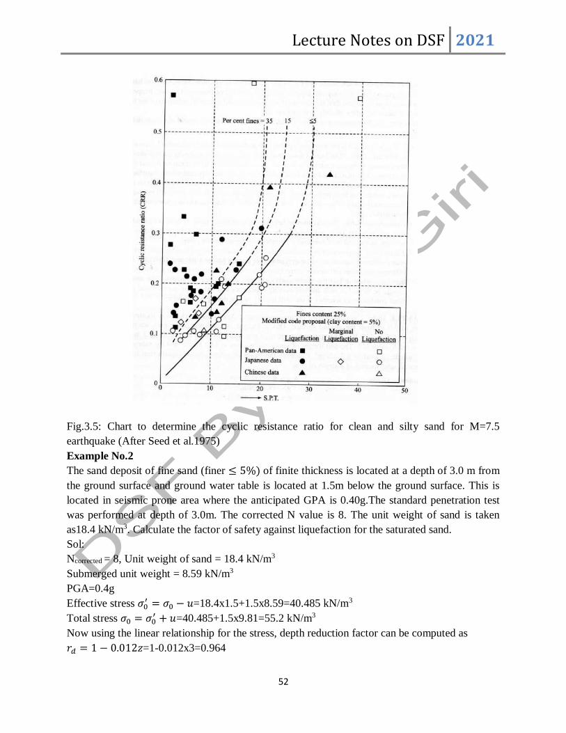
Lecture Notes on DSF 2021
52
Fig.3.5: Chart to determine the cyclic resistance ratio for clean and silty sand for M=7.5
earthquake (After Seed et al.1975)
Example No.2
The sand deposit of fine sand (finer ≤ 5%) of finite thickness is located at a depth of 3.0 m from
the ground surface and ground water table is located at 1.5m below the ground surface. This is
located in seismic prone area where the anticipated GPA is 0.40g.The standard penetration test
was performed at depth of 3.0m. The corrected N value is 8. The unit weight of sand is taken
as18.4 kN/m3. Calculate the factor of safety against liquefaction for the saturated sand.
Sol:
Ncorrected = 8, Unit weight of sand = 18.4 kN/m3
Submerged unit weight = 8.59 kN/m3
PGA=0.4g
Effective stress 𝜎0′ = 𝜎0 − 𝑢=18.4x1.5+1.5x8.59=40.485 kN/m3
Total stress 𝜎0 = 𝜎0′ + 𝑢=40.485+1.5x9.81=55.2 kN/m3
Now using the linear relationship for the stress, depth reduction factor can be computed as
𝑟𝑑 = 1 − 0.012𝑧=1-0.012x3=0.964
Lecture Notes on DSF 2021
53
So CSR=0.65x𝑟𝑑 (𝜎0
𝜎0′) (
𝑎𝑚𝑎𝑥
𝑔)=0.65 × 0, .964 ×
55.2
40.485× 0.4=0.342
Using Fig.4 with Ncorrected=8, CRR can be obtained as 0.09
Hence 𝐹𝑆 =0.09
0.342=0.263
So based on the calculation of factor of safety against liquefaction, the sand deposit liquefy.
Problem No 1:
A 10 m thick loose sand deposit (Dr=42%, finer≤5%) is saturated below a depth of 4 m. The
sand layer region is highly prone to liquefaction. Estimate the ground acceleration that would be
required to produce sand soils in a M=7.5 earthquake.

Lecture Notes on DSF 2021
54
4.0 DYNAMIC SOIL PROPERTIES
4.1 Laboratory Method
The soil properties which are needed in analysis and design of a structure subjected to dynamic
loading are:
(a) Dynamic moduli, such as Young's modulus E, shear modulus G, and bulk modulus K
(b) Poisson's ratio µ
(c) Dynamic elastic constants, such as coefficient of elastic uniform compression Cu, coefficient
of elastic uniform shear, 𝐶𝜏, coefficient of elastic non-uniform Compression 𝐶∅ and coefficient of
elastic non-uniform shear 𝐶𝜑
(d) Damping ratio, ξ
(e) Liquefaction parameters, such as cyclic stress ratio, cyclic deformation and pore pressure
response.
f) Strength-deformation characteristics in terms of strain rate effects.
Since the dynamic properties of soils are strain dependent various laboratory and field techniques
have been developed to measure these properties over a wide range of strain amplitudes.
4.2 LABORATORY TECHNIQUES
The laboratory methods used for determining the dynamic properties of soils are:
i) Resonant column test,
ii) Ultrasonic pulse test,
iii) Cyclic simple shear test,
iv) Cyclic torsional simple shear test, and
v) Cyclic triaxial compression test
4.2.1 Resonant Column Test:
The resonant column test is used to obtain the elastic modulus E, shear modulus G and damping
characteristics of soils at low strain amplitudes. This test is based on the theory of wave
propagation in prismatic rods (Richart, Hall and Woods, 1970). Either a cyclically varying axial
load or torsional load is applied to one end of the prismatic or cylindrical specimen of soil. This
in turn will propagate either a compression wave or a shear wave in the specimen. In this
technique the excitation frequency generating the wave is adjusted until the specimen
experiences resonance. The value of the resonant frequency is used to find the value of E and G
depending on the type of the excitation (axial or torsional).
i) Fixed-free end Condition:
Hall and Richart (1963) described the apparatus with fixed-free end condition. In this
arrangement one end of the specimen is fixed against rotation and the other end is free to rotate
under the applied torsion (Figure 4.1a).Anode occurs at the fixed end and the distribution of
angular rotation 𝜃 along the specimen is a 1
4𝑠𝑖𝑛𝑒wave.
As shown in Figure 4.1b, by adding a mass at the free end, the variation of θ along the specimen
becomes nearly linear. J and J0 are respectively the polar moment of inertias of the specimen and
the added mass respectively. Dmevich (1967) used the concept of added mass to obtain a
uniform strain distribution 'throughout the length of the specimen.
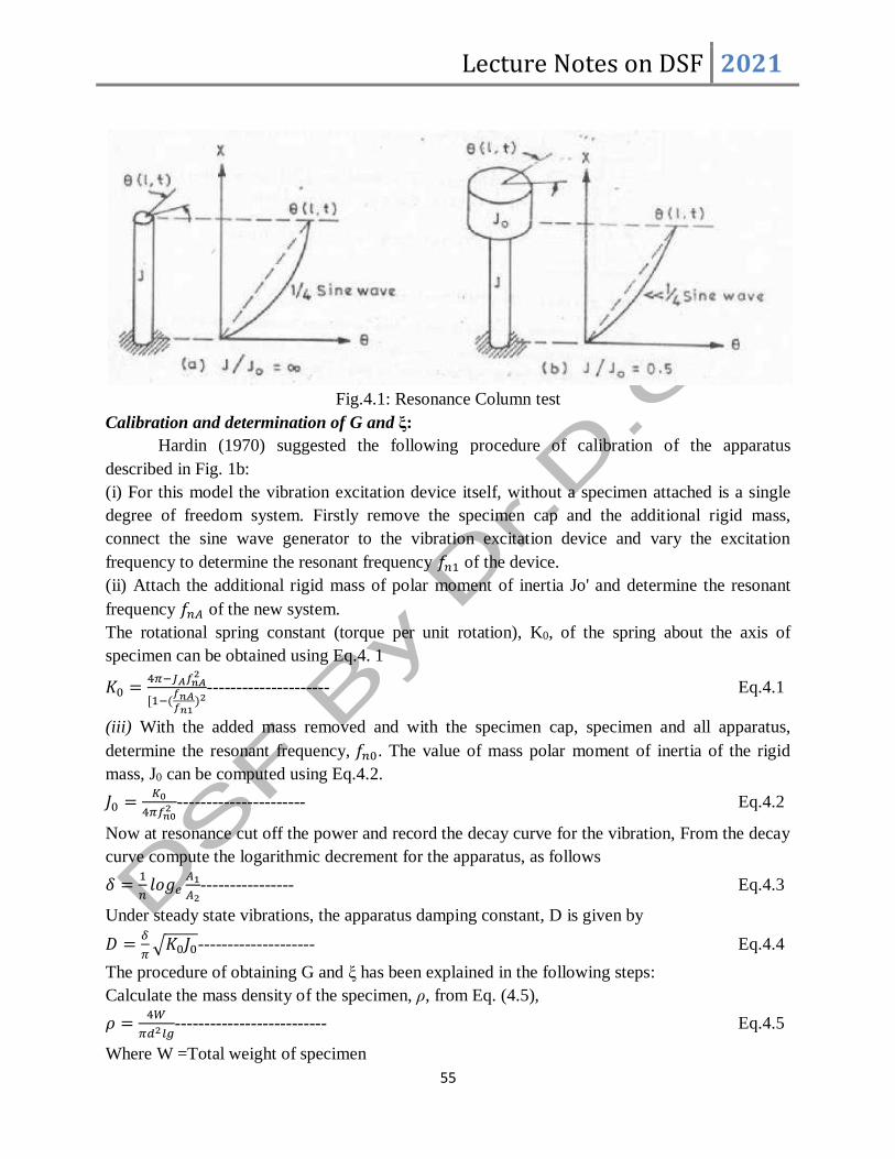
Lecture Notes on DSF 2021
55
Fig.4.1: Resonance Column test
Calibration and determination of G and ξ:
Hardin (1970) suggested the following procedure of calibration of the apparatus
described in Fig. 1b:
(i) For this model the vibration excitation device itself, without a specimen attached is a single
degree of freedom system. Firstly remove the specimen cap and the additional rigid mass,
connect the sine wave generator to the vibration excitation device and vary the excitation
frequency to determine the resonant frequency 𝑓𝑛1 of the device.
(ii) Attach the additional rigid mass of polar moment of inertia Jo' and determine the resonant
frequency 𝑓𝑛𝐴 of the new system.
The rotational spring constant (torque per unit rotation), K0, of the spring about the axis of
specimen can be obtained using Eq.4. 1
𝐾0 =4𝜋−𝐽𝐴𝑓𝑛𝐴
2
[1−(𝑓𝑛𝐴𝑓𝑛1
)2--------------------- Eq.4.1
(iii) With the added mass removed and with the specimen cap, specimen and all apparatus,
determine the resonant frequency, 𝑓𝑛0. The value of mass polar moment of inertia of the rigid
mass, J0 can be computed using Eq.4.2.
𝐽0 =𝐾0
4𝜋𝑓𝑛02 ---------------------- Eq.4.2
Now at resonance cut off the power and record the decay curve for the vibration, From the decay
curve compute the logarithmic decrement for the apparatus, as follows
𝛿 =1
𝑛𝑙𝑜𝑔𝑒
𝐴1
𝐴2---------------- Eq.4.3
Under steady state vibrations, the apparatus damping constant, D is given by
𝐷 =𝛿
𝜋√𝐾0𝐽0-------------------- Eq.4.4
The procedure of obtaining G and ξ has been explained in the following steps:
Calculate the mass density of the specimen, ρ, from Eq. (4.5),
𝜌 =4𝑊
𝜋𝑑2𝑙𝑔-------------------------- Eq.4.5
Where W =Total weight of specimen

Lecture Notes on DSF 2021
56
l= Length of specimen
d = Diameter of specimen
g =Acceleration due to gravity,
(ii) Calculate the inertia of the specimen about its axis J, as follows:
𝐽 = 𝜌𝜋
32𝑑4𝑙-------------------- Eq.4.6
(iii) Calculate the system factor, T as follows:
𝑇 =𝐽0
𝐽−
𝐾0
4𝜋2𝑓𝑛𝑅2 𝐽
-------------------- Eq.4.7
Where J0 = Mass polar moment of inertia of the apparatus
K0 = Rotational spring constant,
J = Inertia of the specimen
fnR = Resonant frequency of the complete system.
iv) To measure the torque current constant, Kt excite the apparatus successively at frequencies
(√2, 2), 𝑓𝑛0√2 and 2𝑓𝑛0, during the steady state vibration at each of these frequencies measure
the current flowing through the coils, C in amperes, and the displacement amplitude of vibration,
θ in radians. For each frequency compute the torque-current constant Kt as follows
𝐾𝑡 =𝐾0𝜃
𝐶𝑀𝑓---------------- Eq.4.8
Where Mf is given in Table 4.1
Frequency 𝑀𝑓
(√2
2)𝑓𝑛0
2
(√2)𝑓𝑛0 1
2𝑓𝑛0 1/3
(iv) Using Figure 4.2, determine the dimensionless frequency F for the value of T computed in
step (ii).
Fig.4.2: System factor T versus F

Lecture Notes on DSF 2021
57
𝐺 = 4𝜋2𝜌[𝑓𝑛𝑅
𝐹𝑙]2----------------- Eq.4.9
For steady state vibration, the damping factor of the system is given as
𝐷𝑠 =1
4𝜋2𝐽2𝑓𝑛𝑅2 ⌈
𝐾𝑡𝐶𝑅
𝜃𝑅− 2𝜋𝐷𝐴𝐹𝑛𝑅⌉-------------- Eq.4.10
CR is the mode shape
4.2.2 Cyclic Triaxial Compression Test
In general the stress-deformation and strength characteristics of a soil depend on the following
factors:
1. Type of soil
2. Relative density in case of cohesionless soils; consistency limits, water content and state
of disturbance in cohesive soils
3. Initial static stress level i.e. sustained stress
4. Magnitude of dynamic stress
5. Number of pulses of dynamic load
6. Frequency of loading
7. Shape of wave form of loading
8. One directional or two directional loading
In one directional loading only compression of the sample is done while in two directional
loading both compression and extension is done. All the factors listed above can be studied
lucidly on a triaxial set up.
Casagrande and Shannon (1948, 1949) developed the following three types of apparatus for
studying the strength of soils under transient loading (Table.4.2)
Table 4.2: Type of Apparatus
Type of apparatus Time of loading (seconds) Remarks
(i) Pendulum loading 0.05 to 0.01 Suitable for
performing fast
transient tests
(ii) Falling beam 0.5 to 300
(iii) Hydraulic loading 0.05 to any desired larger value
Time of loading was defined as the time between the beginning of test and the point at which the
maximum compressive stress is reached (Figure 4.3). The pendulum loading apparatus (Figure 4.
4) utilizes the energy of a pendulum which, when released from a selected height, strikes a spring
connected to the piston rod of a hydraulic lower cylinder. This lower cylinder is connected
hydraulically to an upper cylinder, which is mounted on a loading frame.
i) Pendulum Loading Test: A pendulum loading system was first developed by
Casagrande and Shannon (1948-49). The loading mechanism is based on the
utilization of energy of a pendulum when released from a selected height and striking
a spring connected to the piston rod of a hydraulic cylinder as shown in the Fig.4. 4(a)
ii) The falling beam apparatus consists essentially of a beam with a weight and rider, a
dashpot to control the velocity of the fall of the beam, and a yoke for transmitting the

Lecture Notes on DSF 2021
58
load from the beam to the specimen (Fig. 4.4 b). A small beam mounted above the
yoke counter-balances the weight of the beam.
Fig.4.3 Time of loading in transient tests
iii) Pendulum Loading Test: A pendulum loading system was first developed by
Casagrande and Shannon (1948-49). The loading mechanism is based on the
utilization of energy of a pendulum when released from a selected height and striking
a spring connected to the piston rod of a hydraulic cylinder as shown in the Fig. 4.4(a)
iv) The falling beam apparatus consists essentially of a beam with a weight and rider, a
dashpot to control the velocity of the fall of the beam, and a yoke for transmitting the
load from the beam to the specimen (Fig 4.4 b). A small beam mounted above the
yoke counter-balances the weight of the beam.
v) The hydraulic loading apparatus (Fig. 4.4 c) consists of a constant volume vane-type
hydraulic pump connected to a hydraulic cylinder through valves by which either the
pressure in the cylinder or the volume of the liquid delivered to the cylinder can be
controlled. The peak load that can be produced by this apparatus is much greater than
can be obtained by either the pendulum type or falling beam apparatus.
Fig. 4.4 (a) Pendulum loading apparatus (Casagrande and Shannon. 1948)

Lecture Notes on DSF 2021
59
Fig.4.4 (b) Falling beam apparatus (Casagrande and Shannon. 1948)
Fig. 4.4 c: Hydraulic loading apparatus (Casagrande & Shannon, 1948)
For measuring load, a load gage of rectangular or cylindrical shape is used, with four strain gages
mounted on the inside face. For measuring deflection, a thin flexible steel spring cantilever is
used with strain gages mounted on the cantilever, the base of which is clamped to the loading
piston.
A simultaneous plot of stress and strain versus time from an unconfined compression test with a
time of loading of 0.02 s on cambridge clay is shown in Figure 4.5. Similar plots were prepared
for other times of loading on Manchester sand. Using this data, stress-strain plots were obtained
as shown in Figs.6 a and b. In these figures, stress-strain curves for corresponding static tests are

Lecture Notes on DSF 2021
60
also shown. Typical plots of maximum compressive stress versus time of loading (or unconfined
and confined transient tests on Cambridge clay are shown in Fig. 4.7 a and b respectively. A
typical plot in terms of principal stress ratio a failure and time of loading for Manchester sand is
shown in Fig. 4.8.
Fig.4.5: Time Vs stress and strain in an unconfined transient test on Cambridge clay (Casagrande &
Shannon, 1948)
Fig 4.6 (a): Stress vrs Strain curves
Fig. 4.6(b): Stress Vs Strain Curves (Manchester sand)

Lecture Notes on DSF 2021
61
Fig. 4.7(a): Maximum Compressive Stress (unconfined) versus Time of Loading for Cambridge clay
Fig.4.7 (b): Maximum Compressive Stress (confined) versus Time of Loading for Cambridge
clay
Fig. 4.8: Maximum principal stress ratio versus time of loading for Manchestor sand

Lecture Notes on DSF 2021
62
Modulus of deformation is defined as the slope of a line drawn from the origin through the point
on the stress-deformation curve and corresponding to stress of one-half the strength. It is found
that in case of clays, modulus of deformation in fast transient tests was about two times that
obtained in static tests. In case of sands, modulus of deformation was found independent of the
time of loading.
4.2.3 Summary of Cyclic Tests
In the preceding sections, various types of laboratory test methods were presented, from which
the fundamental soil properties such as the shear modulus, modulus of elasticity, and damping
ratio are determined. These parameters are used in the design and evaluation of the behavior of
earthen, earth-supported, and earth-retaining structures. As was discussed in the preceding
sections, the magnitudes of G and ξ are functions of the shear strain amplitude γ′. Hence, while
selecting the values of G and ξ for a certain design work, it is essential to know the following:
a. Type of test from which the parameters can be obtained
b. Magnitude of the shear strain amplitude at which these parameters needs to be measured For
example, strong ground motion and nuclear explosion can develop large strain amplitudes
whereas some sensitive equipment such as electron microscopes may be very sensitive to small
strain amplitudes.
Figure 9 provides is a useful reference table for geotechnical engineers; as it gives the amplitude
of shear strain levels, type of applicable dynamic tests, and the area of applicability of these test
results. Despite the fact that laboratory testing is not ideal, it will continue to be important
because soil conditions can be better controlled in the laboratory. Parametric studies necessary
for understanding the soil behaviour of soils under dynamic loading conditions must be
performed in the laboratory conditions. Table 4.3 provides a comparison of the relative qualities
(what property can be measured and what is the degree of quality of the measured property) of
various laboratory techniques for measuring dynamic soil properties. Similarly, Table 4.4 gives a
summary of the different engineering parameters that can be measured in different dynamic or
cyclic laboratory tests
Fig. 4.9: Range and applicability of dynamic laboratory tests
Table 4.3: Relative Quality of Laboratory Techniques for Measuring Dynamic Soil Propertiesa

Lecture Notes on DSF 2021
63
Table 4.4: Parameters Measured in Dynamic or Cyclic Laboratory Testsa
4.3 FIELD TEST METHOD
Field methods generally depend on the measurement of velocity of waves propagating through
the soil or on the response of soil structure systems to dynamic excitation. The following
methods are in use for determining dynamic properties of soil:
1. Seismic cross-bore hole survey
2. Seismic up-hole survey
3. Seismic down-hole survey
4. Seismic refraction survey
5. Vertical block resonance test

Lecture Notes on DSF 2021
64
6. Horizontal block resonance test
7. Cyclic plate load test
8. Standard penetration test
4.3.1 Seismic Cross-borehole Survey
This method is based on the measurement of velocity of wave propagation from one borehole to
another. Figure 4.10 shows the essentials of seismic cross-hole method outlined by Stoke and
Woods (1972).A source of seismic energy is generated at the bottom of one borehole and the
time of travel of the shear wave from this borehole to another at known distance is measured.
Shear wave velocity is then computed by dividing the distance between the boreholes by the
travel time.
As discussed above, seismic cross-borehole survey can be done using two boreholes one has the
source for causing wave generation and another having geophone for recording travel time.
However, for extensive investigations and better accuracy, three or more boreholes arranged in a
straight line should be used.
In this case the wave velocities can be calculated from the time intervals between succeeding
pairs of holes, eliminating most of the concern over triggering the timing instruments and the
effects of borehole casing and backfilling (Stokoe and Hour, 1978). Also this arrangement of
bore holes in a straight line overcomes problems of site anisotropy by examining one direction
only at a time.
Fig. 4.10: Multiple hole seismic cross hole survey
4.3.2 Seismic Up-Hole Survey
Seismic up-hole survey is done by using only one borehole. In this method the receiver is placed
at the surface, and shear waves are generated at different depths within the borehole. Figure
4.11shows the schematic presentation of the arrangement used in seismic up-hole survey (Gote et

Lecture Notes on DSF 2021
65
al., 1977).This method gives the average value of wave velocity for the soil between the
excitation and the receivers if one receiver is used, or between the receivers.
The major disadvantage in seismic up-hole survey is that it is more difficult to generate waves of
the desired type.
Fig.4.11: Seismic Up-hole survey
4.3.3 Seismic Down-hole Survey
In this method, seismic waves are generated at the surface of the ground near the top of the
borehole, and travel times of the body waves between the source and the receivers which have
been clamped to the borehole wall at predetermined depths are obtained. The arrangement used
in seismic down-hole survey is shown schematic ally in Figure 4.12. This also requires only one
borehole.
The main advantage of this method is that low velocity layers can be detected even if trapped
between layers of greater velocity provided the geophone spacings are close enough.
4.3.4 Vertical Block Resonance Test
The vertical block resonance test is used for determining the values of coefficient of elastic
uniform compression (Cu), Young's modulus (E) and damping ratio (ξ) of the soil.
According to IS 5249: 1984, a test block of size 1.5 m x 0.75 m x 0.70 m high is casted in
M15concrete in a pit of plan dimensions 4.5 m x 2.75 m and depth equal to the proposed depth of
foundation. Foundation bolts should be embedded into the concrete block at the time of casting
for fixing the oscillator assembly. The oscillator assembly is mounted on the block so that it
generates purely vertical sinusoidal vibrations. The line of action of vibrating force should pass
through the centre of gravity of the block. Two acceleration or displacement pickups are
mounted on the top of the block as shown in Figure 4.13 such that they sense the vertical motion
of the block. A schematic diagram of the set up is shown in Figure 4.13.
The mechanical oscillator works on the principle of eccentric masses mounted on two shafts
rotating in opposite directions. The force generated by the oscillator is given by
𝐹𝑑 = 2𝑚𝑒𝑒2𝜔--------------- Eq.4.11

Lecture Notes on DSF 2021
66
Fig. 4.12: Seismic Down-hole survey
Fig.4.13: Set-up for block resonance test
The oscillator is first set at a particular eccentricity (e).As evident from Eq. (4.11) higher the
eccentricity more will be the force level. It is then operated at constant frequency and the
acceleration of the oscillatory motion of the block is monitored. The oscillator frequency is
increased in steps, and the signals of monitoring pickups are recorded. At any eccentricity and
frequency the dynamic force should not exceed 20 percent of the total mass of the block and
oscillator assembly. The amplitude of vibration (AZ) at a given frequency is given by
𝑨𝒁 =𝒂𝒛
𝟒𝝅𝟐𝒇𝟐-------------------------- Eq.4.12
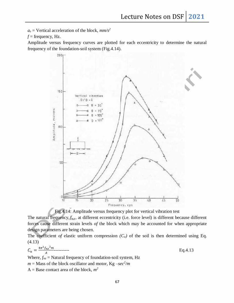
Lecture Notes on DSF 2021
67
az = Vertical acceleration of the block, mm/s2
f = frequency, Hz.
Amplitude versus frequency curves are plotted for each eccentricity to determine the natural
frequency of the foundation-soil system (Fig.4.14).
Fig.4.14: Amplitude versus frequency plot for vertical vibration test
The natural frequency,𝑓𝑛𝑧, at different eccentricity (i.e. force level) is different because different
forces cause different strain levels of the block which may be accounted for when appropriate
design parameters are being chosen.
The coefficient of elastic uniform compression (Cu) of the soil is then determined using Eq.
(4.13)
𝐶𝑢 =4𝜋2𝑓𝑛𝑧
2𝑚
𝐴---------- Eq.4.13
Where, fnz = Natural frequency of foundation-soil system, Hz
m = Mass of the block oscillator and motor, Kg –sec2/m
A = Base contact area of the block, m2

Lecture Notes on DSF 2021
68
From the value of Cu obtained from Eq. (3) for the test block of contact area A the value of Cu1
for the actual foundation having contact area A1 may be obtained from Eq. (4.14)
𝐶𝑢1 = 𝐶𝑢√𝐴
𝐴1---------------- Eq.4.14
The Eq. (4.14) is valid for base areas of foundations up to 10 m2. For areas larger than 10 m2,
the value Cu obtained for 10 m2 is used.
The value of damping ratio ξ is determined using Eq. (4.15) as
𝜉 =𝑓2−𝑓1
2𝑓𝑛𝑧---------------- Eq.4.15
Where, f1, f2= Two frequencies at which amplitudes is equal to 𝐴𝑚𝑎𝑥
√2
Amax= Maximum amplitude
fnz = Resonant frequency
The coefficient of elastic uniform compression (Cu) is related to the elastic Young's modulus (E)
by Eq (6) which is in the form of Boussinesq relationship for the elastic settlement of a surface
footing.
𝐶𝑢 =𝐸
1−𝜇2𝐶𝑠
√𝐵𝐿------------------- Eq.4.16
where 𝜇 = Poisson's ratio
B = Width of base of the block
L = Length of base of the block
Cs = Coefficient depending on 𝐿 𝐵⁄ ratio
Barkan (1962) recommended the values of Cs for various 𝐿 𝐵⁄ ratios as listed in Table 4.5
Table 4.5: values of Cs for various 𝐿 𝐵⁄ ratios
𝐿𝐵⁄ Cs
1.0 1.06
1.5 1.07
2.0 1.09
3.0 1.13
5.0 1.22
10.0 1.41
The value of damping ratio ξ is determined using Eq. (4.17) as
𝜉 =𝑓2−𝑓1
2𝑓𝑟𝑧--------------------------- Eq.4.17
Where, f1,f2 = Two frequencies at which amplitudes is equal to 𝐴𝑚𝑎𝑥
√2
Amax = Maximum amplitude
frz= Resonant frequency
Example No.1

Lecture Notes on DSF 2021
69
A vertical vibration test was conducted on a 1.5m x 0.75 m x 0.70 m high concrete block in an
open pit having depth 2.0 which is equal to the anticipated depth of actual foundation. The test
was repeated at different settings (e) of eccentric masses.
The data obtained from the tests are given below:
Sl.No θ(degree) 𝑓𝑛𝑧 Amplitude at Resonance
(Micron)
1 36 41.0 13.0
2 72 40.0 24.0
3 108 34.0 32.0
4 144 31.0 40.0
The soil is sandy in nature having angle of internal friction is 35° and saturated density is 20 kN/
m3). The water table lies at a depth of 3.0 m below the ground surface. Probable size of the actual
foundation is 4.0 x 3.0 x 3.5 m high. Determine the values of Cu, E and G to be adopted for the
design of actual foundation.
Limiting vertical amplitude of the machine is 150 microns.
Sol:
1 Area of Block=1.5x0.75=1.125 m2
Mass of Block=1.125x0.75x2400=1890 kg
Mass of oscillator and motor=100 kg (assumed)
Mass of block, oscillator and motoa=1890+100=1990 kg
2 𝐶𝑢 =4𝜋2𝑓𝑛𝑧
2𝑚
𝐴=
4𝜋2×𝑓𝑛𝑧2×1990
1.125×100= 69.84𝑓𝑛𝑧
2𝑘𝑁/𝑚2
The calculated values of 𝐶𝑢 for different observed resonance frequencies are tabulated as
shown in Table 1
Cu can be evaluated from Eq.4.6 as𝐶𝑢 =𝐸
1−𝜇2𝐶𝑠
√𝐵𝐿 for L/B=2 CS=1.09
Assume µ=0.35, 𝐸 =√1.125(1−0.352)
1.09× 𝐶𝑢=0.854𝐶𝑢𝑘𝑁/𝑚
2
𝐺 =𝐸
2(1+𝜇)=
0.854𝐶𝑢
2(1+0.35))=0.316𝐶𝑢 𝑘𝑁/𝑚
2
For different values of 𝐶𝑢, E and G values are calculated and tabulated as shown in table 1
3 Correction for confining pressure and area
The mean effective confining pressure 𝜎01 at depth of' one -half the width below the centre
of block is given by
𝜎01 = 𝜎𝑣 (1 + 2𝐾0)
3
Where 𝜎𝑣 = 𝜎𝑣1 + 𝜎𝑣2
𝜎𝑣1 =Effective overburden pressure at the depth under consideration
𝜎𝑣2 =Increase in vertical pressure due to the weight of block
Assuming that the top 2.0 m soil has a moist unit weight of 18 kN/m3, and the next 1.0 m soil
i.e. up to water table is saturated then
𝜎𝑣1 = 18 × 2.0 + 20 ×0.70
2= 43𝑘𝑁/𝑚2

Lecture Notes on DSF 2021
70
𝜎𝑣2 =4𝑞
4𝜋[2𝑚𝑛√𝑚2 + 𝑛2 + 1
𝑚2 + 𝑛2 + 1 +𝑚2𝑛2×𝑚2 + 𝑛2 + 2
𝑚2 + 𝑛2 + 1+ 𝑠𝑖𝑛−1
2𝑚𝑛√𝑚2 + 𝑛2 + 1
𝑚2 + 𝑛2 + 1 +𝑚2𝑛2]
𝑚 =𝐿/2
𝑍=
1.5/2
0.7/2=2.14
𝑛 =𝐵/2
𝑍=
0.75/2
0.7/2=1.07
Where q=24x0.7=16.8 𝑘𝑁/𝑚2
Substituting for the values of m and n, we get
𝜎𝑣2 = 13.44𝑘𝑁/𝑚2
Now 𝜎𝑣 = 𝜎𝑣1 + 𝜎𝑣2 = 43 + 13.44 = 56.44𝑘𝑁/𝑚2
𝐾0 = 1 − 𝑠𝑖𝑛∅ = 0.426
𝜎01 = 𝜎𝑣 (1 + 2𝐾0)
3= 56.44 ×
1 + 2 × 0.426
3= 34.84𝑘𝑁/𝑚2
For the actual foundation, 𝜎𝑣1 =18x2.0+20x1.0+ (20-10)x0.5= 61 𝑘𝑁
𝑚2
𝑚 =4.0/2
3.0/2= 1.33
𝑛 =3.0/2
3.0/2= 1.0
𝑞 = 24 × 3.5 = 84𝑘𝑁
𝑚2
Substituting the values of m, n and q we get
𝜎02 =124.76[1+2×0.426
3] = 77.01
𝑘𝑁
𝑚2
Area of actual foundation =4.0x0.3=12.0 m2 (> 10𝑚2)
Hence, 𝐶𝑢2
𝐶𝑢1=
𝐸2
𝐸1=𝐺2
𝐺1= (
𝜎02
𝜎01 )0.5
× (𝐴1
𝐴2)0.5
= (77.0
34.84)0.5
× (1.125
10)0.5
= 0.4986
For actual foundation Cu =0.4986x Cu for block
Table 1:
Sl.
No
θ
in
deg.
𝑓𝑛𝑧 Amplitude
at
Resonance
(micron)
For Test Block For Actual Foundation
Cu
104kN/m2
E 104kN/m2
G 104kN/m2
Cu
104kN/m2
E 104kN/m2
G 104kN/m2
1 36 41 13 11.74 10.03 3.71 5.85 5.00 1.85
2 72 40 24 11.17 9.54 3.53 5.57 4.76 1.77
3 108 34 32 7.15 6.11 2.26 3.56 3.05 1.13
4 144 31 40 6.71 5.73 2.12 3.35 2.86 1.06
Strain Level Correction
The values of strain levels corresponding to values of Cu = amplitude at resonance per width of
test block are given as
Sl.No Cu (Test Block) Strain Level(10-4)
1 11.74 0.173 (13x10-6/0.75)
2 11.17 0.320 (24x10-6/0.75)

Lecture Notes on DSF 2021
71
3 7.15 0.427 (32x10-6/0.75)
4 6.71 0.533 (40x10-6/0.75)
Strain in Actual foundation=150×10−6
3.0= 0.5 × 10⁻⁴
The value of Cu, E and G corresponding to actual strain level of foundation can be obtained by
interpolation as
𝐶𝑢 = [3.56 − (3.56 − 3.35)0.5−0.427
0.533−0.427] × 104= 2.31x10⁴ kN/m2
𝐸 = [3.05 − (3.05 − 2.86)0.5−0.427
0.533−0.427] × 104 =1.97x10⁴ kN/m2
𝐺 = [1.13 − (1.13 − 1.06)0.5−0.427
0.533−0.427] × 104= 0.73x10⁴ kN/m2
4.3.5 Horizontal Block Resonance Test
Horizontal block resonance test is also performed on the block set up as shown in Figure 4.14. In
this test, the mechanical oscillator is mounted on the block so that horizontal sinusoidal
vibrations are generated in the direction of the longitudinal axis of the block. Three acceleration
or displacement pickups are mounted along the vertical centre line of the transverse face of the
block to sense horizontal vibrations (Fig.4.14 a). The oscillator is excited in steps starting from
rest condition. The signal of each acceleration pick up is amplified and recorded. Rest of the
procedure is same as described for vertical block resonance test. Similar tests can be performed
by exciting the block in the direction of transverse axis.
The amplitude of Horizontal vibrations (Ax) is obtained using Eq. (4.18).
𝐴𝑥 =𝑎𝑥
4𝜋2𝑓2------------------------------- Eq.4.18
Where, ax(mm) = Horizontal acceleration in the direction under consideration in mm/s2
f = Frequency in Hz
Amplitude versus frequency curves are plotted for each force level to obtain the natural
frequency, fnz of the block soil system as done in vertical resonance test. A typical frequency
versus amplitude plot is shown in Figure 4.15. It may be noted that the case of horizontal
vibration is a problem of two degrees of freedom.

Lecture Notes on DSF 2021
72
Fig.4.14 Experimental set up
Fig.4.15: Amplitude versus frequency plots for horizontal resonance test

Lecture Notes on DSF 2021
73
The coefficient of elastic uniform shear 𝐶𝜏 of soil is given as
𝐶𝜏 =8𝜋2𝑟𝑓𝑛𝑥
2
(𝐴0+𝐼0)±√(𝐴0+𝐼0)2−4𝑟𝐴0𝐼0
--------------------- Eq.4.19
Where 𝑟 =𝑀𝑚
𝑀𝑚0
𝑓𝑛𝑥 = Horizontal resonant frequency of block soil system
𝐴0 =𝐴
𝑀-
A = Contact area of block with soil
M = Mass of block, oscillator and soil
𝐼0 = 3.46𝐼
𝑀𝑚𝑜------------------------------------- Eq.4.20
Mm = Mass moment of inertia of block, oscillator, motor, etc. about the horizontal axis passing
through the centre of gravity of block and perpendicular to the direction of vibration
Mmo = Mass moment of inertia of the block, oscillator; motor etc. about the horizontal axis
passing through centre of contact area of block and soil and perpendicular to the direction of
vibration.
I = Moment of inertia of the foundation contact area about the horizontal axis passing through
the centre of gravity of area and perpendicular to the direction of vibration.
In Eq. (4.19), negative sign is taken when the system vibrates in first mode and positive sign
when the system vibrates in second mode. For the size of the block recommended in IS 5249-
1977 and for first natural frequency, the Eq. (4.19) reduces to
𝐶𝜏 = 92.3𝑓𝑛𝑥2 ----------------- Eq.4.21 unit of 𝐶𝜏 in this equation is kN/m2
The coefficient of elastic uniform shear (Cτ1) for actual area of foundation (A1) is given by
𝐶𝜏1 = 𝐶𝜏√𝐴
𝐴1-------------------- Eq.4.22
IS 5249: 1977 recommends the following relations between Cu and 𝑪𝝉, Cφ and Cψ
Cu = 1.5 to 2.0 𝐶𝜏 -------------- Eq.4.23
𝐶∅= 3.46 𝐶𝜏 ------------------- Eq.4.24
𝐶𝜓= 0.75 Cu-------------------- Eq.4.25
4.3.6 Cyclic Plate Load Test
The cyclic plate load test is performed in a test pit dug up to the proposed base level of
foundation. The equipment is same as used in static plate load test. Circular or square bearing
plates of mild steel not less than 25 mm thickness and varying in size from 300 to 750 mm with
grooved bottom are used. The test pit should be at least five times the width of the plate. The
equipment is assembled according to details given in IS 1988-1982. A typical set up is shown in
Figure 4.16.

Lecture Notes on DSF 2021
74
Fig. 4.16: Experimental set up for Cyclic Plate Load test
To commence the test, a seating pressure of about 7 kPa is first applied to the plate. It is then
removed and dial gauges are set to read zero. Load is then applied in equal cumulative
increments of not more than 100 kPa or of not more than one fifth of the estimated allowable
bearing pressure. In cyclic plate load test, each incremental load is maintained constant till the
settlement of the plate is complete. The load is then released to zero and the plate is allowed to
rebound. The reading of final settlement is taken. The load is then increased to next higher
magnitude of loading and maintained constant till the settlement is complete, which is recorded.
The load is then reduced to zero and the settlement reading is taken. The next increment of load
is then applied. The cycles of unloading and reloading are continued till the required final load
is reached.
The data obtained from a cyclic plate load test is shown in Figure 4.17. From this data, the load
intensity versus elastic rebound is plotted as shown in Figure 4.18, and the slope of the line is
coefficient of elastic uniform compression.

Lecture Notes on DSF 2021
75
𝐶𝑢 =𝑃
𝑆𝑒(𝑘𝑁 𝑚3⁄ )------------------ Eq.4.26
Where P=Load Intensity in kN/m2
Se= Elastic rebound corresponding to P in mm
Fig. 4.17: Load Intensity versus Settlement Fig.4.19: Load Intensity versus Elastic rebound
It can be shown theoretically (Barkan, 1962) that
𝐶𝑢 =𝑃
𝑆𝑒= 1.13
𝐸
1−𝜇21
√𝐴---------------- Eq.4.27
Where Cu= Sub-grade modulus, E = Modulus of elasticity, μ = Poisson’s ratio and A = area of
the plate.
However 𝐺 =𝐸
2(1+𝜇)
So, 𝐶𝑢 = 2.26𝐺(1+𝜇)
1−𝜇21
√𝐴------------ Eq.4.28
OR, 𝐺 =(1−𝜇)𝐶𝑢√𝐴
2.26----------------- Eq.4.29
The magnitude of Cu can be obtained from the plot of q versus se (Figure 4). With the known
value of A and a representative value of μ, the shear modulus can be calculated from Eq. (12). In
non homogenous soils, it may be desirable to conduct the test at different depths or one may use
different plate sizes to reflect the change in soil stiffness with depth. Again, it should be noted
that this test suffers from the same limitations as reported in traditional geotechnical engineering
practice for the design of foundations.

Lecture Notes on DSF 2021
76
Example 1
The plot of q versus s (settlement) obtained from a cyclic plate load test is shown in Figure
below. The area of the plate used for the test was 0.3 m2. Calculate
a. Kplate, and
b. Shear modulus G (assume μ = 0.35).
Sol: From the settlement curve the following can be
determined
From the graph
𝐶𝑢 =𝑃
𝑆𝑒=
300
0.0021= 142.86𝑀𝑁 𝑚3⁄
𝐾𝑝𝑙𝑎𝑡𝑒 =𝑞𝐴
𝑆𝑒= 142.86 × 0.3
= 42.86𝑀𝑁/𝑚
𝐺 =(1 − 𝜇)𝐶𝑢√𝐴
2.26=(1 − 0.35)142.86 × √0.3
2.26= 22.5𝑀𝑃𝑎
4.3.7 Standard Penetration Test
The standard penetration test (SPT) is the most extensively used situ test in India and many other
countries. This test is carried in a bore hole using a split spoon sampler. As per IS: 2131-1981,
steps involved in carrying out this test are as follows:
(i) The borehole is made to the depth at which the SPT has to be performed. The bottom of the
borehole is cleaned.
(ii) The split-spoon sampler, attached to standard drill rods of required length is lowered into the
borehole and rested at the bottom.
(iii) The split –spoon sampler is seated 150 mm by blows of a drop hammer of 65 kg falling
vertically and
Lecture Notes on DSF 2021
77
Freely from a height of 750 mm. Thereafter, the split spoon sampler shall be further driven 300
mm in two steps each of 150 mm. The number of blows required to effect each 150 mm of
penetration shall be recorded. The first 150 mm of drive may be considered to be seating drive.
The total blows required for the second and third 150 mm of penetration is termed the
penetration resistance N.
If the split spoon sampler is driven less than 450 mm (total), then N-value shall be for the last
300 mm penetration. In case, the total penetration is less than 300 mm for 50 blows, it is entered
as refusal in the bore log.
(iv) The split spoon sampler is then withdrawn and is detached from the drill rods. The split
barrel is disconnected from the cutting shoe and the coupling. The soil sample collected inside
the barrel is collected carefully and preserved for transporting the same to the laboratory for
further tests.
(v) Standard penetration tests shall be conducted at every change in stratum or intervals of not
more than 1.5 m whichever is less. Tests may be done at lesser intervals (usually 0.75 m) if
specified or considered necessary.
The penetration test in gravelly soils requires careful interpretation since pushing a piece of
gravel can greatly change the blow count.
4.3.7.1 Corrections to observed SPT values (N) in cohesionless soils
Following two types of corrections are normally applied to the observed SPT values (N) in
cohesionless soils:
i) Corrections due to dilatancy:
In very fine, or silty, saturated sand, Terzaghi and Peck (1967) recommend that the observed N-
values be
Corrected to N' if N was greater than 15 as
𝑁′ = 15 +1
2(𝑁 − 15)------------------------Eq.4.30
Bazaraa (1967) recommended the correction as
N' = 0.6N (for N > 15) -------------------- Eq.4.31
This correction is introduced with the view that in saturated dense sand (N > 15); the fast rate of
application of shear through the blows of drop hammer, is likely to induce negative pore
pressures and thus temporary increase in shear strength will occur. This will lead to a N-value
higher than the actual one. Since sufficient experimental evidence is not available to confirm this
correction, many engineers are not applying this correction. However this correction has also
been recommended in IS: 2131-1981.
ii) Correction due to overburden pressure:
On the basis of field tests, corrections to the N-value for overburden effects were proposed by
many investigators (Gibbs and Holtz 1957; Teng 1965; Bazaraa 1967; Peck, Hanson and
Thornburn 1974). The methods which are normally used are:
Bazaraa (1967)
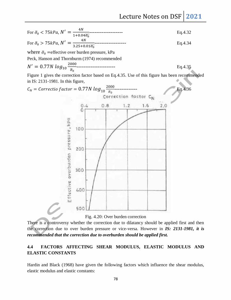
Lecture Notes on DSF 2021
78
For ��0 < 75𝑘𝑃𝑎, 𝑁′ =4𝑁
1+0.04𝜎0------------------- Eq.4.32
For ��0 > 75𝑘𝑃𝑎, 𝑁′ =4𝑁
3.25+0.01𝜎0------------------ Eq.4.34
where ��0 =effective over burden pressure, kPa
Peck, Hanson and Thornburm (1974) recommended
𝑁′ = 0.77𝑁𝑙𝑜𝑔102000
��0---------------------- Eq.4.35
Figure 1 gives the correction factor based on Eq.4.35. Use of this figure has been recommended
in IS: 2131-1981. In this figure,
𝐶𝑁 = 𝐶𝑜𝑟𝑟𝑒𝑐𝑡𝑖𝑜𝑓𝑎𝑐𝑡𝑜𝑟 = 0.77𝑁𝑙𝑜𝑔102000
��0------------- Eq.4.36
Fig. 4.20: Over burden correction
There is a controversy whether the correction due to dilatancy should be applied first and then
the correction due to over burden pressure or vice-versa. However in IS: 2131-1981, it is
recommended that the correction due to overburden should be applied first.
4.4 FACTORS AFFECTING SHEAR MODULUS, ELASTIC MODULUS AND
ELASTIC CONSTANTS
Hardin and Black (1968) have given the following factors which influence the shear modulus,
elastic modulus and elastic constants:

Lecture Notes on DSF 2021
79
(i) Type of soil including grain characteristics, grain shape, grain size, grading and mineralogy;
(ii) Void ratio
(iii) Initial average effective confining pressure;
(iv) Degree of saturation;
(v) Frequency of vibration and number of cycles of load
(vi) Ambient stress history and vibration history
(vii) Magnitude of dynamic stress; and
(viii) Time effects
Soil behavior over a wide range of strain amplitudes is nonlinear and on unloading follows a
different stress-strain path forming a hysteresis loop as shown in Figure 4.21. The area inside this
loop represents the energy absorbed by the soil during its deformation and is a measure of the
internal damping within the soil.
At very low strain amplitudes (≪ 0.0001 %) the soil acts essentially as a linear elastic material
with little or no loss of energy. The shear modulus under these conditions is maximum, but as the
strain amplitude is increased, the shear modulus decreases and the damping within the soil
increase.
Fig.4.21: Stress-strain loop at different cycles of loading after Headley, 1985

Lecture Notes on DSF 2021
80
5.0 DESIGN OF MACHINE FOUNDATIONS
5.1 Categories of machine foundations
Reciprocating machines:
It produces periodic unbalanced force and operating frequency is 600rpm. For designing
unbalanced force is taken as varying sinusoidally.
Impact machines:
It produces impact loads at an operating frequency of 60-150 blows/min. Dynamic load attends
the peak within short duration and then die out quickly. Designed as over tuned.
Rotary machines:
These are high speed machines with high operating frequency. Hence the foundations are
designed as under tuned.
5.2 TYPES OF MACHINE FOUNDATIONS
Block type
Caisson type
Frame type
Fig.5.1: Types of machine foundations
• Block type machine foundation is a solid block made of concrete block of huge mass,
area and depth. The pedestal machine will be positioned on the top of the block.
• Box or caisson type is used to save some material of concrete in order to avoid an
uneconomic design when the foundation requirement is huge size as well as height of the
foundation is more.
• Framed foundation are used when the machine are subjected to very high operating
frequency like turbo generator etc.
5.3 CRITERIA FOR THE DESIGN OF MACHINE FOUNDATIONS

Lecture Notes on DSF 2021
81
• These foundations should be well design to take care of the static loads coming on the
foundation.
• No shear or bearing capacity failure should occur. That means, the bearing capacity of the
foundation against shear failure is to be checked.
• No excessive settlement, that is amount of settlement as calculated under static load and
that has to be compared with different codal guidelines.
• Under the dynamic loading condition, the foundation should not resonate.
• The natural frequency of foundation soil must be far away from machine to avoid the
resonance.
• Dynamic displacement amplitude must not exceed the permissible limit.
• Vibration of the machine and foundation system together must not be annoying to the
person working in the environment and it should not damage the adjacent structures.
• Machine foundation should not design for a strong foundation to take care of the dynamic
load but also safe against bearing capacity failure, as well as safe against the resonance
criteria.
5.3.1 Suggested Foundation for Various Types of Machines
1. Machine producing Impulse: Block type foundation
Example: hammer, Presses etc
2. Rotating type machine with low to medium frequency: Block type foundation with large
contact area.
Example: Large reciprocating engine, Compressor, large blower
3. Rotating type machine with medium to high frequency: Block type foundation resting on
suitable elastic pad or spring.
Example: Medium sized reciprocating engine, diesel engine and gas engine
4. Rotating type with very high frequency: Framed foundation or massive block with
minimum contact area.
Example: internal combustion engine, electric motors, turbo-generators
5.4 METHODS OF ANALYSIS
Linear elastic weightless spring MSD model
Linear elastic theory
Indian standard design code: IS 2974, Part 1 provisions
Machine foundation has to be designed by checking three criteria.
1 Dimensional criteria,
2 Vibration criteria
3 Displacement criteria
These are the three major criteria, which needs to be checked to design a machine foundation as
per our Indian standard design code 2974.
5.4.1 Check the Dimension
For a block type of foundation, the criteria given that size of the foundation block must be larger
than the base plate of the machine.

Lecture Notes on DSF 2021
82
The second criteria says minimum all-around clearance of 150 mm. must be provided as per IS
codal provision.
A third criterion is that, the foundation block should be placed deep enough on good bearing
strata.
The combined centre of gravity of the machine plus foundation block should be as far below the
top of the foundation as possible.
5.4.2 Vibration Check
Foundation which is having natural frequency either much higher or lower than the operating
frequency of the machine, is called under tuned or over tuned respectively.
If the ratio of operating frequency to the natural frequency is less than or equal to 0.5 that can be
designed as Under tuned criterion.
If the operating frequency is much higher than the natural frequency and frequency ratio
𝜉 =𝜔
𝜔𝑛> 2 for important machine and
𝜉 =𝜔
𝜔𝑛> 1.5for less important machine
For both types of machine design criteria is Over tuned.
• To design machine for which operating frequency is very high, over tuned criteria is used
because an under tuned type of foundation design result will provide negative value of
mass or no mass because of the value of k which has to be excessively high.
• To design machine for which operating frequency is low, under tuned criteria is used.
• However for the range of say 1000 rpm or even in the range of 600 rpm, it is always
better to check your design for both over tuned and under tuned.
5.4.3 Displacement Criteria
• The amplitude of permissible dynamic displacement should be less than or equals to 0.2
mm, If it exceeds, foundation is to be redesigned.
• The permissible displacement should be checked using Richart’s chart. So, that it should
not become annoying to the workers or adjacent structures.
• Y-axis of the chart shows dynamic displacement amplitude and X axis represents
operating frequency of the machine.
Fig.5.2: Displacement amplitude vs. frequency (Richard 1962

Lecture Notes on DSF 2021
83
5.5 LINEAR ELASTIC WEIGHTLESS SPRING MSD MODEL
𝜔𝑛𝑧 = √𝐾𝑧𝑚
Vertical
Vibration
𝜔𝑛𝑥 = √
𝐾𝑥𝑚
Horizontal
Vibration
𝜔𝑛∅ = √𝐾𝑛∅𝑀𝑚0
Rocking Mode
𝜔𝑛𝜑 = √
𝐾𝑛𝜑
𝑀𝑚𝑧
Yawing Mode
Coefficient of uniform elastic compression, Cu
𝐶𝑢 =𝑃
𝑆𝑒---------------------- Eq.5.1
Where P and Se are the load corresponding to elastic settlement
Coefficient of linear elastic shear, 𝐶𝜏 =𝜏
𝑆𝑒------------------------ Eq.5.2
Barken (1962) proposed the following values:
Cu=2Cz , Cφ=2Cu , 𝐶𝜏 = 1.5𝐶𝜑------------------------- Eq.5.3
According to IS: 5249:
𝐶𝑢 = 1.73𝐶𝜏 and 𝐶𝜏 = 1.5𝐶𝜑------------------------------- Eq.5.4
Vertical Vibration of the Block
Load applied: 𝑃𝑧 = 𝑃0𝑠𝑖𝑛𝜔𝑡--------------------------------- Eq.5.5
Equation of motion: 𝑚�� + 𝐾𝑧𝑍 = 𝑃0𝑠𝑖𝑛𝜔𝑡-------------------- Eq.5.6
Natural Frequency =𝜔𝑛𝑧 = √𝐶𝑢𝐴
𝑚------------------------ Eq.5.7
Amplitude of Vertical Vibration, 𝐴𝑧 =𝑃𝑂𝑠𝑖𝑛𝜔𝑡
𝑚(𝜔𝑛𝑧2 −𝜔2)
----------------- Eq.5.8
Maximum Amplitude of Vibration =𝑃𝑧
𝑚(𝜔𝑛𝑧2 −𝜔2)
--------------------- Eq.5.9
Sliding Vibration of the Block
Load applied: 𝑃𝑥 = 𝑃0𝑠𝑖𝑛𝜔𝑡------------------------ Eq.5.10
Equation of motion: 𝑚�� + 𝐾𝑧𝑥 = 𝑃0𝑠𝑖𝑛𝜔𝑡----------------- Eq.5.11
Natural Frequency =𝜔𝑛𝑥 = √𝐶𝑢𝐴
𝑚------------------------ Eq.5.12
Amplitude of Vertical Vibration, 𝐴𝑥 =𝑃𝑂𝑠𝑖𝑛𝜔𝑡
𝑚(𝜔𝑛𝑧2 −𝜔2)
----------------- Eq.5.13
Maximum Amplitude of Vibration =𝑃𝑥
𝑚(𝜔𝑛𝑧2 −𝜔2)
------------------ Eq.5.14

Lecture Notes on DSF 2021
84
5.4.3 LINEAR ELASTIC THEORY
(Based on Elastic Half Space Theory)
In 1904, Lamb studied the problem of vibration of single vibrating force acting at a point on the
surface of an elastic half-space. This study included cases in which the oscillating force R acts in
the vertical direction and in the horizontal direction, as shown in Figure 5.3 a and b. This is
generally referred to as the dynamic Boussinesq problem.
In 1936, Reissner analyzed the problem of vibration of a uniformly loaded flexible circular area
resting on an elastic half-space. The solution was obtained by integration of Lamb’s solution for
a point load. Based on Reissner’s work, the vertical displacement at the center of the flexible
loaded area (Figure 5.4 a) can be given by
𝑍 =𝑄𝑂𝑒
𝑖𝜔𝑡
𝐺𝑟0(𝑓1 + 𝑖𝑓2)----------------------- Eq.5.15
Where Q0=amplitude of the exciting force acting on the foundation
Z= periodic displacement at the centre of the loaded area
𝜔= circular frequency of the applied load
𝑟0 = radius of the loaded area
G= shear modulus of the soil
𝑓1, 𝑓2=Reissner’s displacement functions
Fig. 5.3: Vibrating force on the surface of elastic half -space

Lecture Notes on DSF 2021
85
Fig.5.4: a) Vibration of uniformly loaded circular flexible area, b) Flexible circular area
subjected to force vibration
The displacement functions𝑓1and 𝑓2 are related to the Poisson’s ratio of the medium and the
frequency of the exciting force. Now, consider a flexible circular foundation of weight W (mass
= m = W/g) resting on an elastic half-space and subjected to an exciting force of magnitude of
(𝑄0𝑒𝑖(𝜔𝑡+𝛼) as shown in Figure 5.4b. (Note: α is the phase difference between the exciting force
and the displacement of the foundation.)
Using the displacement relation given in Eq. (5.15) and solving the equation of equilibrium of
force, Reissner obtained the following relationships:
𝐴𝑧 =𝑄0
𝐺𝑟0𝑍---------------------- Eq.5.16
Where Az = the amplitude of vibration
Z= dimensionless amplitude
=√𝑓12+𝑓2
2
(1−𝑏𝑎02𝑓1)
2+(𝑏𝑎02𝑓2))
2--------------------- Eq.5.17
b= dimensionless mass ratio
=𝑚
𝜌𝑟03 =
𝑊
𝑔[
1
(𝛾𝑔⁄ )𝑟0
3] =𝑊
𝛾𝑟03--------------------- Eq.5.18
ρ= density of the elastic material
γ=unit of soil

Lecture Notes on DSF 2021
86
a0=dimensionless frequency=𝜔𝑟0√𝜌
𝐺=
𝜔𝑟0
𝑉𝑠------------------ Eq.5.19
Vs= velocity of shear wave in the elastic material on which the foundation is resting
The classical work of Reissner was further extended by Quinlan (1953) and Sung (1953). As
mentioned before, Reissner’s work related only to the case of flexible circular foundations where
the soil reaction is uniform over the entire area (Figure 5.5a). Both Quinlan and Sung considered
the cases of rigid circular foundations, the contact pressure of which is shown in Figure 5.3b,
flexible foundations (Figure 5.5a), and the types of foundations for which the contact pressure
distribution is parabolic, as shown in Figure 5.5c. The distribution of contact pressure q for all
three cases may be expressed as follows.
For flexible circular foundations
𝑞 =𝑄0𝑒
𝑖(𝜔𝑡+𝛼)
𝜋𝑟02 for 𝑟 ≤ 𝑟0--------------------- Eq.5.20
For rigid circular foundations
𝑞 =𝑄0𝑒
𝑖(𝜔𝑡+𝛼)
2𝜋𝑟0√𝑟02−𝑟2
(𝑓𝑜𝑟𝑟 ≤ 𝑟0)--------------------- Eq.5.21
For foundations with parabolic contact pressure distribution
𝑞 =2(𝑟0
2−𝑟2)𝑄0𝑒𝑖(𝜔𝑡+𝛼)
𝜋𝑟04 (𝑓𝑜𝑟𝑟 ≤ 𝑟0)----------------------- Eq.5.22
a) Uniform pressure distribution b) pressure distribution c) parabolic pressure
under rigid foundation distribution
Fig. 5.5: Contact pressure distribution under circular footing of radius r0
Quinlan derived the equations only for the rigid circular foundation; however, Sung presented
the solutions for all the three class described. For all cases, the amplitude of motion can be
expressed in a similar form to Eqs. (5.2 to 5.5). However, the displacement functions 𝑓1and
𝑓2will change, depending on the contact pressure distribution.
Foundations, on some occasions, may be subjected to a frequency dependent excitation, in
contrast to the constant-force type of excitation just discussed. Figure 5.6 shows a foundation
excited by two rotating masses. The amplitude of the exciting force can be given as

Lecture Notes on DSF 2021
87
𝑄 = 2𝑚𝑒𝑒𝜔2 = 𝑚1𝑒𝜔
2----------------------- Eq.5.23
Where m1= total of the rotating masses
ω= circular frequency of the rotating masses
Fig. 5.6: Foundation vibration by a frequency dependent exciting force
For the above condition, the amplitude of vibration Az can be expressed as
𝐴𝑧 =𝑚1𝑒𝜔
2
𝐺𝑟0√
𝑓12+𝑓2
2
(1−𝑏𝑎02𝑓1)
2+(𝑏𝑎02𝑓2))
2----------------- Eq.5.24
Where 𝑎0 = 𝜔𝑟0√𝜌
𝐺-------------------------------- Eq.5.25
𝜔2 =𝐺𝑎0
2
𝜌𝑟02-------------------------------------- Eq.5.26
Substituting Eq. 5.26 into Eq. 5.24 we get
𝐴𝑧 =𝑚1𝑒𝑎0
2
𝜌𝑎03 √
𝑓12+𝑓2
2
(1−𝑏𝑎02𝑓1)
2+(𝑏𝑎0
2𝑓2))2=
𝑚1𝑒
𝜌𝑟03 𝑍
′------------- Eq.5.27
Where 𝑍′ = 𝑎02√
𝑓12+𝑓2
2
(1−𝑏𝑎02𝑓1)
2+(𝑏𝑎02𝑓2))
2-------------------- Eq.5.28
Figures 5.7 and 5.8 show the plots of the variation of the dimensionless amplitude with a0
(Richart, 1962) for rigid circular foundations (for μ = Poisson’s ratio = 0.25 and b = 5, 10, 20,
and 40).

Lecture Notes on DSF 2021
88
Fig. 5.7: Plot of Z versus a0 for rigid circular Fig. 5.8: Variation of Z′ with a0 for
foundation , Richart, 1962) rigid circular foundation (redrawn
after Richart, 1962)
5.4.4 Effect of Contact Pressure Distribution and Poisson’s Ratio
The effect of the contact pressure distribution on the nature of variation of the non-dimensional
amplitude Z′ with a0 is shown in Figure 5.9 (for b = 5 and μ = 0.25). As can be seen, for a given
value of a0, the magnitude of the amplitude is highest for the case of parabolic pressure
distribution and lowest for rigid bases.
For a given type of pressure distribution and mass ratio (b), the magnitude of Z′ also greatly
depends on the assumption of the Poisson’s ratio μ. This is shown in Figure 5.10.

Lecture Notes on DSF 2021
89
Fig. 5.9: Effect of contact pressure distribution variation of Z’ with a0 (redrawn after Richart and
Whitman, 1967)
Fig.5.10: Effect of Poisson’s ratio on the variation of Z’ with a0 (redrawn after Richart and
Whitman, 1967)
5.4.5 Variation of Displacement Functions f1 and f2
As mentioned before, the displacement functions are related to the dimensionless frequency a0
and Poisson’s ratio μ. In Sung’s original study, it was assumed that the contact pressure
distribution remains the same throughout the range of frequency considered; however, for
dynamic loading conditions, the rigid-base pressure distribution does not produce uniform
displacement under the foundation. For that reason, Bycroft (1956) determined the weighted

Lecture Notes on DSF 2021
90
average of the displacements under a foundation. The variation of the displacement functions
determined by the study is shown in Figure 5.11
Fig.5.11: Variation of the displacement functions with a0 and μ
5.5 Analog Solutions for Vertical Vibration of Foundations
Lysmer’s Analog
A simplified model was also proposed by Lysmer and Richart (1966), in which the expressions
for kz and Cz were frequency independent. Lysmer and Richart (1966) redefined the
displacement functions in the form
𝐹 =𝑓
[1−𝜇
4]=
𝑓1+𝑖𝑓2
[1−𝜇
4]= 𝐹1 + 𝑖𝐹2------------------ Eq.5.29
The functions F1 and F2 are practically independent of Poisson’s ratio, as shown in Figure 5.11.
The term mass ratio as expressed in Eq. (5.18) was also modified as
𝐵𝑧 = [1−𝜇
4] 𝑏 = [
1−𝜇
4]𝑚
𝜌𝑟03------------------------- Eq.5.30
Where Bz = modified mass ratio
In this analysis, it was proposed that satisfactory results can be obtained within the range of
practical interest by expressing the rigid circular foundation vibration in the form
𝑚�� + 𝐶𝑧�� + 𝐾𝑧𝑍 = 𝑄0𝑒𝑖𝑤𝑡-------------------- Eq.5.31
Where

Lecture Notes on DSF 2021
91
𝐾𝑧 = 𝑠𝑡𝑎𝑡𝑖𝑐𝑠𝑝𝑟𝑖𝑛𝑔𝑐𝑜𝑛𝑠𝑡𝑎𝑛𝑡𝑓𝑜𝑟𝑟𝑖𝑔𝑖𝑑𝑐𝑖𝑟𝑐𝑢𝑙𝑎𝑟𝑓𝑜𝑢𝑛𝑑𝑎𝑡𝑖𝑜𝑛 =4𝐺𝑟0
1−𝜇--------- Eq.5.32
And
𝐶𝑧 =3.4𝑟0
2
1−𝜇√𝐺𝜌---------------------------- Eq.5.33
Fig.5.12: Plot of F1 and -F2 against a0 for rigid circular foundation subjected to vertical
vibration (after Lysmer and Richart, 1966)
In Eqs. (5.32) and (5.33) the relationships for Kz and Cz are frequency independent. Equations
(5.31 to 5.33) are referred to as Lysmer’s analog.
5.6 CALCULATION PROCEDURE FOR FOUNDATION RESPONSE, VERTICAL
VIBRATION
Once the equation of motion of a rigid circular foundation is expressed in the form given in
Equation (5.31), it is easy to obtain the resonant frequency and amplitude of vibration based on
Lecture Notes on DSF 2021
92
the mathematical expressions presented in earlier section. The general procedure is outlined
next.
A. Resonant Frequency
1. Calculation of natural frequency. as
𝑓𝑛 =1
2𝜋√𝐾𝑧
𝑚=
1
2𝜋√
4𝐺𝑟0
(1−𝜇)𝑚-------------------- Eq.5.34
2. Calculation of damping ratio ξ. As given
Critical damping 𝐶𝑐 = 2√𝐾𝑧𝑚 = 2√4𝐺𝑟0
(1−𝜇)𝑚, substituting for m as 𝑚 =
4𝐵𝑧𝜌𝑟03
(1−𝜇)
= 4√(4𝐺𝑟0
(1−𝜇))(
𝐵𝑧𝜌𝑟03
(1−𝜇)) =
8𝑟02
(1−𝜇)√𝐺𝜌𝐵𝑧------------------------ Eq.5.35
Now , 𝜉 =𝐶
𝐶𝐶=
3.4𝑟02
1−𝜇√𝐺𝜌
8𝑟02
(1−𝜇)√𝐺𝜌𝐵𝑧
=0.425
√𝐵𝑧-------------------------- Eq.5.36
3. Calculation of the resonance frequency (that is, frequency at maximum displacement). For
constant force-type excitation,
𝑓𝑚 = 𝑓𝑛√1− 2𝜉2
=1
2𝜋√
4𝐺𝑟0
(1−𝜇)𝑚× √1− 2(
0.425
√𝐵𝑧)2--------------------- Eq.5.37
It has also been shown by Lysmer that, for Bz ≥ 0.3, the following approximate relationship can
be established:
𝑓𝑚 =1
2𝜋√(
𝐺
𝜌)(
1
𝑟0) × √
𝐵𝑧−0.36
𝐵𝑍----------------------- Eq.5.38
For rotating mass-type excitation, Lysmer’s corresponding approximate relationship for fm is as
follows:
𝑓𝑚 =1
2𝜋√(
𝐺
𝜌)(
1
𝑟0) × √
0.9
𝐵𝑍−0.45------------------------- Eq.5.39
B. Amplitude of Vibration at Resonance
The amplitude of vibration Az at resonance for constant force-type excitation can be determined
as
𝐴𝑧𝑟𝑒𝑠𝑜𝑛𝑎𝑛𝑐𝑒 = (𝑄𝑧
𝐾𝑧)
1
2𝜉𝑧√1−𝜉𝑧2----------------- Eq.5.40
Now substituting for Kz and 𝜉𝑧 we obtain
𝐴𝑧𝑟𝑒𝑠𝑜𝑛𝑎𝑛𝑐𝑒 =𝑄0(1−𝜇)
4𝐺𝑟0×
𝐵𝑧
0.85√𝐵𝑍−0.18------------------------ Eq.5.41
The amplitude of vibration for rotating mass-type vertical excitation can be given as [see Eq.
(2.99)]
𝐴𝑧𝑟𝑒𝑠𝑜𝑛𝑎𝑛𝑐𝑒 =𝑚1𝑒
𝑚×
𝐵𝑧
0.85√𝐵𝑍−0.18--------------------- Eq.5.42
C. Amplitude of Vibration at Frequencies Other Than Resonance
For constant force-type excitation, can be used for estimation of the amplitude of vibration, or

Lecture Notes on DSF 2021
93
𝐴𝑧 =𝑄0
𝐾𝑧⁄
√(1−𝜔2
𝜔𝑛2 )
2
+4(𝜉𝑧)2(
𝜔
𝜔𝑛)2------------------- Eq.5.43
Figure 5.13 shows the plot of 𝐴𝑧
𝑄0𝐾𝑧⁄
versus (𝜔
𝜔𝑛 ). So, with known values of 𝜉𝑧 and (
𝜔
𝜔𝑛 ), one can
determine the value of 𝐴𝑧
𝑄0𝐾𝑧⁄
and, from that, Az can be obtained.
In a similar manner, for rotating mass-type excitation, Eq. (2.95) can be used to determine the
amplitude of vibration, or
𝐴𝑧 =(𝑚𝑒𝑒
𝑚⁄ )(𝜔 𝜔𝑛⁄ )2
√(1−𝜔2
𝜔𝑛2)
2
+4(𝜉𝑧)2(
𝜔
𝜔𝑛)2----------------------------- Eq.5.44
Fig.5.13: Plot of various non-dimensional parameters against (𝜔 𝜔𝑛⁄ ) for constant force-type
vibrator (Note: ξ = ξz for vertical vibration, ξ = ξθ for rocking, ξ = ξx for sliding; ξ = ξα for
torsional vibration.)

Lecture Notes on DSF 2021
94
Fig.5.14: Plot of various non-dimensional parameters against (𝜔 𝜔𝑛⁄ ) for rotating mass-type
vibrator (Note: ξ = ξz for vertical vibration, ξ = ξθ for rocking, ξ = ξx for sliding; ξ = ξα for
torsional vibration.)
The procedure here described relates to a rigid circular foundation having a radius of r0. If a
foundation is rectangular in shape with length L and width B, it is required to obtain an
equivalent radius, which can then be used in the preceding relationships as discussed in above.
This can be done by equating the area of the given foundation to the area of an equivalent circle.
Thus,
𝜋𝑟02 = 𝐿𝐵
where r0 = radius of the equivalent circle.
It is obviously impossible to eliminate vibration near a foundation.
However, an attempt can be made to reduce the vibration problem as much as possible. Richart
(1962) compiled guidelines for allowable vertical vibration amplitude for a particular frequency
of vibration, and this is given in Figure 5.15.
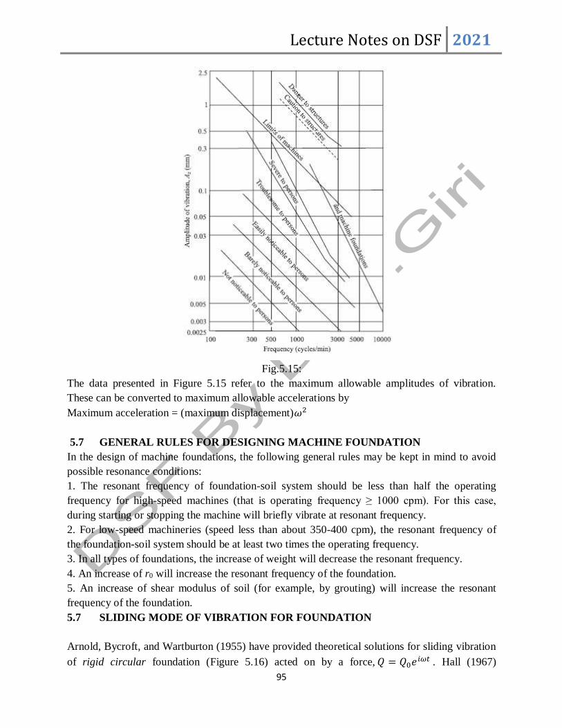
Lecture Notes on DSF 2021
95
Fig.5.15:
The data presented in Figure 5.15 refer to the maximum allowable amplitudes of vibration.
These can be converted to maximum allowable accelerations by
Maximum acceleration = (maximum displacement)𝜔2
5.7 GENERAL RULES FOR DESIGNING MACHINE FOUNDATION
In the design of machine foundations, the following general rules may be kept in mind to avoid
possible resonance conditions:
1. The resonant frequency of foundation-soil system should be less than half the operating
frequency for high-speed machines (that is operating frequency ≥ 1000 cpm). For this case,
during starting or stopping the machine will briefly vibrate at resonant frequency.
2. For low-speed machineries (speed less than about 350-400 cpm), the resonant frequency of
the foundation-soil system should be at least two times the operating frequency.
3. In all types of foundations, the increase of weight will decrease the resonant frequency.
4. An increase of r0 will increase the resonant frequency of the foundation.
5. An increase of shear modulus of soil (for example, by grouting) will increase the resonant
frequency of the foundation.
5.7 SLIDING MODE OF VIBRATION FOR FOUNDATION
Arnold, Bycroft, and Wartburton (1955) have provided theoretical solutions for sliding vibration
of rigid circular foundation (Figure 5.16) acted on by a force,𝑄 = 𝑄0𝑒𝑖𝜔𝑡 . Hall (1967)

Lecture Notes on DSF 2021
96
developed the mass-spring-dashpot analog for this type of vibration. According to this analog,
the equation of motion of the foundation can be given in the form
𝑚�� + 𝐶𝑥�� + 𝐾𝑥𝑥 = 𝑄0𝑒𝑖𝜔𝑡------------------------ Eq.5.45
where m= mass of the foundation
Fig.5.16: Sliding mode of vibration of rigid circular foundation
Spring constant for horizontal mode of vibration
𝐾𝑥 =32.4(1−𝜇)𝐺𝑟0
7−8𝜇------------------ Eq.5.46
Dash pot coefficient for horizontal mode of vibration
𝐶𝑥 =18.4(1−𝜇)𝑟0
2
7−8𝜇√𝜌𝐺---------------------- Eq.5.47
The natural frequency of the foundation for sliding can be calculated as
𝑓𝑛 =1
2𝜋√𝐾𝑥
𝑚=
1
2𝜋√32(1−𝜇)𝐺𝑟0
(7−8𝜇)𝑚-------------------------- Eq.5.48
The critical damping and damping ratio in sliding can be evaluated as
𝐶𝑐𝑥 = critical damping in sliding
𝐶𝑐𝑥 = 2√𝐾𝑥𝑚 = 2√32(1−𝜇)𝐺𝑟0
(7−8𝜇)𝑚-------------------- Eq.5.48
ξx = damping ratio in sliding
𝜉𝑥 =𝐶𝑥
𝐶𝑐𝑥=
0.288
√𝐵𝑋----------------- Eq.5.49
Where , Bx is the dimensionless mass ratio expressed as
𝐵𝑥 =7−8𝜇
32(1−𝜇)
𝑚
𝜌𝑟03-------------------------- Eq.5.50
Calculation Procedure for Foundation Response Using Eq. (5.51)
Resonant Frequency
1. Calculate the natural frequency fn using Eq. (5.45)
2. Calculate the damping ratio ξx using Eq. (5.49). [Note: Bx can be obtained from Eq. (5.50)].

Lecture Notes on DSF 2021
97
3. For constant force excitation (that is, Q0 = constant), calculate
𝑓𝑚 = 𝑓𝑛√1 − 2𝜉𝑥2--------------------------Eq.5.51
4. For rotating mass type excitation, calculate
𝑓𝑚 =𝑓𝑛
√1−2𝜉𝑥2--------------------------------------Eq.5.52
Amplitude of Vibration at Resonance
1. For constant force excitation, amplitude of vibration at resonance is
𝐴𝑥(𝑟𝑒𝑠𝑜𝑛𝑎𝑛𝑐𝑒) =𝑄0
𝐾𝑥
1
2𝜉𝑥√1−𝜉𝑥2-----------------------Eq.5.53
2. For rotating mass-type excitation
𝐴𝑥(𝑟𝑒𝑠𝑜𝑛𝑎𝑛𝑐𝑒) =𝑚𝑒𝑒
𝑚
1
2𝜉𝑥√1−𝜉𝑥2---------------------Eq.5.54
where m1 = total rotating mass causing excitation
e = eccentricity of each rotating mass
Amplitude of Vibration at Frequency Other than Resonance
1. For constant force-type excitation
𝐴𝑧 =𝑄0
𝐾𝑥⁄
√(1−𝜔2
𝜔𝑛2 )
2
+4(𝜉𝑥)2(
𝜔
𝜔𝑛)2--------------------------- Eq.5.55
2. For rotating mass-type excitation,
𝐴𝑧 =(𝑚𝑒𝑒
𝑚⁄ )(𝜔 𝜔𝑛⁄ )2
√(1−𝜔2
𝜔𝑛2 )
2
+4(𝜉𝑥)2(
𝜔
𝜔𝑛)2------------------------------ Eq.5.56
Same figures 5.13 & 5.14 are used to calculate various non-dimensional parameters against
(𝜔 𝜔𝑛⁄ ) for constant force and rotating mass-type vibrator respectively.
5.8 TORSIONAL VIBRATION OF FOUNDATIONS
Figure 5.21a shows a circular foundation of radius r0 subjected to a torque 𝑇 = 𝑇0𝜃𝑖𝜔𝑡 about an
axis z-z. The vibration problem of this type was solved by Reissner (1937) solved considering a
linear distribution of shear stress 𝜏𝑧𝜃(shear stress zero at center and maximum at the periphery
of the foundation), as shown in Figure 5.17b which represents the case of a flexible foundation.

Lecture Notes on DSF 2021
98
Fig.5.17 Torsional variation of rigid circular foundation
In 1944 Reissner and Sagoli solved the same problem for the case of a rigid foundation
considering a linear variation of displacement from the center to the periphery of the foundation.
Similar to the cases of vertical, rocking, and sliding modes of vibration, the equation for the
torsional vibration of a rigid circular foundation can be written as
𝐽𝑧𝑧�� + 𝐶𝛼�� + 𝐾𝛼𝛼 = 𝑇0𝑒𝑖𝜔𝑡------------------------- Eq.5.57
Where, Jzz= mass moment of inertia of the foundation about the axis z-z
Cα = dashpot coefficient for torsional vibration
Kα = static spring constant for torsional vibration = 16
3𝐺𝑟0
3
α = rotation of the foundation at any time due to the application of a torque 𝑇 = 𝑇0𝑒𝑖𝜔𝑡
The damping ratio ξα for this mode of vibration has been determined as (Richart, Hall, and
Wood, 1970) given below
𝜉𝛼 =0.5
1+2𝐵𝛼----------------------- Eq.5.58
Where
Bα = the dimensionless mass ratio for torsion at vibration=𝐽𝑧𝑧
𝜌𝑟05---------------- Eq.5.59
Calculation Procedure for Foundation Response Using Eq. (5.51)
Resonant Frequency
1. Calculate the natural frequency fn
𝑓𝑛 =1
2𝜋√𝐾𝛼
𝐽𝑧𝑧--------------------- Eq.5.60
2. Calculate the damping ratio Bα using Eq. (5.59) and damping ratio 𝜉𝛼 by Eq. 5.58
3. For constant force excitation (that is, T0 = constant), calculate
𝑓𝑚 = 𝑓𝑛√1 − 2𝜉𝛼2--------------------------Eq.5.61

Lecture Notes on DSF 2021
99
4. For rotating mass type excitation, calculate
𝑓𝑚 =𝑓𝑛
√1−2𝜉𝛼2--------------------------------------Eq.5.62
Amplitude of Vibration at Resonance
1. For constant force excitation, amplitude of vibration at resonance is
𝛼(𝑟𝑒𝑠𝑜𝑛𝑎𝑛𝑐𝑒) =𝑇0
𝐾𝛼
1
2𝜉𝛼√1−𝜉𝛼2-----------------------Eq.5.63
2. For rotating mass-type excitation
𝛼(𝑟𝑒𝑠𝑜𝑛𝑎𝑛𝑐𝑒) =𝑚𝑒𝑒(
𝑥2⁄ )
𝐽𝑧𝑧
1
2𝜉𝛼√1−𝜉𝛼2---------------------Eq.5.64
where m1 = total rotating mass causing excitation
e = eccentricity of each rotating mass
Amplitude of Vibration at Frequency Other than Resonance
3. For constant force-type excitation
𝛼 =𝑇0
𝐾𝛼⁄
√(1−𝜔2
𝜔𝑛2 )
2
+4(𝜉𝛼)2(
𝜔
𝜔𝑛)2--------------------------- Eq.5.65
4. For rotating mass-type excitation,
𝛼 =(𝑚𝑒𝑒(
𝑥2⁄ )
𝐽𝑧𝑧⁄ )(𝜔 𝜔𝑛⁄ )
2
√(1−𝜔2
𝜔𝑛2 )
2
+4(𝜉𝛼)2(
𝜔
𝜔𝑛)2------------------------------ Eq.5.66
For constant force excitation, calculate 𝜔 𝜔𝑛⁄ and then refer to Figure 5.13 to obtain α/(T0/Kα).
For rotating mass-type excitation, calculate 𝜔 𝜔𝑛⁄ and then refer to Figure 5.14 to obtain α/[m1
e(x/2)/Jzz].
For a rectangular foundation with dimensions B × L, the equivalent radius may be given by
𝑟0 = √𝐵𝐿(𝐵2+𝐿2)
6𝜋-------------------- Eq.5.67
The torsional vibration of foundations is uncoupled motion and hence can be treated
independently of any vertical motion. Also, Poisson’s ratio does not influence the torsional
vibration of foundations
5.9 ROCKING VIBRATION OF FOUNDATIONS
A theoretical solution for foundations subjected to rocking vibration was presented by Arnold,
Bycroft, and Wartburton (1955) and Bycroft (1956). Rocking mode of vibration for rigid
circular foundations is shown in Figure 5.18.

Lecture Notes on DSF 2021
100
Fig. 5.18: Rocking vibration of a circular rigid foundation
A mass-spring-dashpot model for rigid circular foundations was developed by Hall (1967) in the
same manner as Lysmer and Richart (1966) developed for vertical vibration. According to Hall,
the equation of motion for a rocking vibration can be given as
𝐼0�� + 𝐶𝜃�� + 𝐾𝜃𝜃 = 𝑀𝑦𝑒𝑖𝜔𝑡------------------- Eq.5.68
Where θ = rotation of the vertical axis of the foundation at any time t
I0 = mass moment of inertia about the y axis (through its base)=𝑊0
𝑔(𝑟02
4+
ℎ2
3)------- Eq.5.69
where W0= weight of the foundation
g = acceleration due to gravity
h = height of the foundation
Static spring constant, 𝐾𝜃 =8𝐺𝑟0
3
3(1−𝜇)------------------- Eq.5.70
Dashpot coefficient, 𝐶𝜃 =0.8𝑟0
4
(1−𝜇)(1+𝐵𝜃)√𝐺--------------------- Eq.5.71
Inertia ratio, 𝐵𝜃 = (3(1−𝜇)
8)
𝐼0
𝜌𝑟05--------------------------- Eq.5.72

Lecture Notes on DSF 2021
101
A. Resonant Frequency
1. Calculate the natural frequency:𝑓𝑛 =1
2𝜋√𝐾𝜃
𝐼0------------------------ Eq.5.73
2. Calculate the damping ratio ,
Critical damping coefficient, 𝐶𝑐𝜃 = 2√𝐾𝜃𝐼0---------------------- Eq.5.74
𝜉𝜃 =0.15
(1+𝐵𝜃)√𝐵𝜃--------------------------- Eq.5.75
3. Calculate the resonant frequency:
𝑓𝑚 = 𝑓𝑛√1− 2𝜉𝜃2 ----(for constant force excitation)----------- Eq.5.76
𝑓𝑚 =𝑓𝑛
√1−2𝜉𝜃2 -----------(for rotating mass-type excitation)---------------- Eq.5.77
B. Amplitude of Vibration at Resonance
Constant force type vibration
𝜃𝑟𝑒𝑠𝑜𝑛𝑎𝑛𝑐𝑒 =𝑀𝑦
𝐾𝜃
1
2𝜉𝜃√1−𝜉𝜃2--------------------- Eq.5.78
For rotating type excitation
𝜃𝑟𝑒𝑠𝑜𝑛𝑎𝑛𝑐𝑒 =𝑚1𝑒𝑍
′
𝐼𝜃
1
2𝜉𝜃√1−𝜉𝜃2--------------------- Eq.5.79
Where, m1 = total rotating mass causing excitation
e = eccentricity of each mass
C. Amplitude of Vibration at Frequencies Other than Resonance
For constant force-type excitation
𝜃 =
𝑀𝑦𝐾𝜃
⁄
√(1−𝜔2
𝜔𝑛2)
2
+4(𝜉𝛼)2(
𝜔
𝜔𝑛)2----------------- Eq.5.80
For rotating mass type vibration

Lecture Notes on DSF 2021
102
𝜃 =(𝑚1𝑒𝑧
,
𝐼0⁄ )(𝜔 𝜔𝑛⁄ )
2
√(1−𝜔2
𝜔𝑛2)
2
+4(𝜉𝛼)2(
𝜔
𝜔𝑛)2---------------------- Eq.5.81
In the case of rectangular foundation, the preceding relationships can be used by determining the
equivalent radius as
𝑟0 = √𝐵𝐿3
3𝜋
4-------------- Eq.5.82
Table 5.1: Values of various Lysmer’s Analog Parameters
Mode of
Vibration
Equivalent
Radius
Mass ratio Damping factor Spring Constant
Vertical 𝑟0 = √𝐵𝐿
𝜋 𝐵𝑧 =
(1 − 𝜇)𝑚
4𝜌𝑟03 𝜉𝑍 =
0.425
√𝐵𝑧 𝐾𝑧 =
4𝐺𝑟01 − 𝜇
Horizontal
𝑟0 = √𝐵𝐿
𝜋
𝐵𝑥 =7 − 8𝜇
32(1 − 𝜇)
𝑚
𝜌𝑟03 𝜉𝑥 =
0.288
√𝐵𝑋 𝐾𝑥 =
32.4(1 − 𝜇)𝐺𝑟07 − 8𝜇
Torsional 𝑟0 = √
𝐵𝐿(𝐵2+ 𝐿2)
6𝜋 𝐵𝛼 =
𝐽𝑧𝑧
𝜌𝑟05 𝜉𝛼 =
0.5
1 + 2𝐵𝛼 𝐾𝛼 =
16
3𝐺𝑟0
3
Rocking 𝑟0 = √
𝐵𝐿3
3𝜋
4
𝐵𝜃 = (
3(1 − 𝜇)
8)𝐼0𝜌𝑟0
5 𝜉𝜃 =0.15
(1 + 𝐵𝜃)√𝐵𝜃 𝐾𝜃 =
8𝐺𝑟03
3(1 − 𝜇)
Example No.1: A concrete foundation is 2.5 m in diameter. The foundation is supporting a
machine. The total weight of the machine and the foundation is 270 kN. The machine imparts a
vertical vibrating force Q = Q0 𝑠𝑖𝑛𝜔𝑡. Given
Q0=27 kN (not frequency dependent). The operating frequency is 150 cpm. For the soil
supporting the foundation, unit weight = 19.5 kN/m3, shear modulus = 45000 kPa. , and Poisson’
ratio = 0.3. Determine:
a. resonant frequency,
b. the amplitude of vertical vibration at resonant frequency, and
c. the amplitude of vertical vibration at the operating frequency
Sol:
The machine imparts a vertical vibrating force Q = Q0 𝑠𝑖𝑛𝜔𝑡 where Q0=27 kN
The operating frequency = 150 cpm=2.5 Hz
Equivalent radius 𝑟0 = 1.25𝑚
Total weight of the machine and the foundation =270 kN
Mass ratio
𝐵𝑧 =(1−𝜇)𝑚
4𝜌𝑟03 =
(1−𝜇)𝑊
4𝛾𝑟03 =
(1−0.3)×270
4×19.5×1.253=1.24
Damping factor

Lecture Notes on DSF 2021
103
𝜉𝑍 =0.425
√𝐵𝑧=0.425
√1.24= 0.382
Spring constant
𝐾𝑧 =4𝐺𝑟0
1−𝜇=4×4500×1.25
1−0.3=32142.86 kN/m2
Natural frequency 𝑓𝑛 =1
2𝜋√
4𝐺𝑟0
(1−𝜇)𝑚=
1
2𝜋√
4×4500×1.25
(1−0.3)×270 9.81⁄=5.44 Hz
a) Resonance frequency 𝑓𝑚 = 𝑓𝑛√1− 2𝜉2=5.44× √1 − 2 × 0.3822=4.58 Hz
b) Amplitude of vertical vibration at resonant frequency:
𝐴𝑧𝑟𝑒𝑠𝑜𝑛𝑎𝑛𝑐𝑒 =𝑄0(1−𝜇)
4𝐺𝑟0×
𝐵𝑧
0.85√𝐵𝑍−0.18=
27(1−0.3)
4×4500×1.25×
1.24
0.85√1.24−0.18=
c) The amplitude of vertical vibration at the operating frequency:
𝐴𝑧 =𝑄0
𝐾𝑧⁄
√(1−𝜔2
𝜔𝑛2 )
2
+4(𝜉𝑧)2(
𝜔
𝜔𝑛)2=
2732142.86⁄
√(1−2.52
5.442)2
+4(0.382)2(2.5
5.44)2
=
Example No.2:
A radar antenna foundation is shown below. For torsional vibration of the foundation, given
T0 = 250 kN-m (due to inertia)
T0 = 83 kN-m (due to wind)
Mass moment of inertia of the tower about the axis z-z = 13 × 106 kg·m2, and the unit weight of
concrete used in the foundation = 24 kN/m3. Calculate
a) the resonant frequency for torsional mode of vibration; and
b) angular deflection at resonance.
Fig: Foundation for radar of antenna
Solution:

Lecture Notes on DSF 2021
104
a)
Damping factor
b) Angular frequency at resonance
Angular deformation due to torque produced by inertia

Lecture Notes on DSF 2021
105

Lecture Notes on DSF 2021
106
5.10 DYNAMIC BEARING CAPACITY OF SHALLOW FOUNDATION
During the application of single pulse dynamic loads which may be in vertical or horizontal
directions, the foundation may get excessive settlement. Horizontal dynamic loads on
foundations are due mostly to earthquakes. These types of loading may induce large
permanent deformation in foundations. Isolated column footings, strip footings, mat footings,
and even pile foundations all may fail during seismic events. Such failures are generally
attributed to liquefaction. However, a number of failures have occurred where field
conditions indicate there was only partial saturation or a dense soil and therefore liquefaction
alone is a very unlikely explanation. Rather, the reason for the seismic settlements of these
foundations seems to be that the bearing capacity was reduced (Richards, Elms and
Budhu,1993).
During the analysis of the time dependent motion of a foundation subjected to dynamic
loading or estimating the bearing capacity under dynamic conditions several factors need to
be considered.
Most important of these factors are
a) Nature of variation of the magnitude of the loading pulse,
b) Duration of the pulse, and
c) Strain-rate response of the soil during deformation
5.10.1 Ultimate Dynamic Bearing Capacity
Bearing Capacity in Sand
The equations for static ultimate bearing capacity evaluation are valid for dense sands where
the failure surface in the soil extends to the ground surface. This is referred as the case of
general shear failure. For shallow foundations (i.e., 𝐷𝑓
𝐵⁄ ≤ 1), if the relative density of
granular soils RD is less than about 70%, local or punching shear failure may occur. Hence,
for static ultimate bearing capacity calculation, if 0 ≤ RD ≤ 0.67, the values of internal angle
of friction, φ should be replaced by the modified friction angle
∅′ = 𝑡𝑎𝑛−1[(0.67+ 𝑅𝐷 − 0.75𝑅𝐷2)𝑡𝑎𝑛∅]------- Eq.5.83
However, when load is applied rapidly to a foundation to cause failure, the ultimate bearing
capacity changes by somewhat. This fact has been shown experimentally by Vesic, Banks,
and Woodward (1965), who conducted several laboratory model tests with a 101.6 mm
diameter rigid rough model footing placed on the surface of a dense river sand (i.e., Df = 0),
both dry and saturated. The rate of loading to cause failure was varied in a range of 2.54 ×
10-4 mm/s to over 254 mm/s. Hence, the rate was in the range of static (2.54 × 10⁻⁴ mm /s) to
impact (254 mm/s) loading conditions. All but the four Based on the experimental results
available, the following general conclusions regarding the ultimate dynamic bearing capacity
of shallow foundations in sand can be drawn:
1. For a foundation resting on sand and subjected to an acceleration level of amax ≤ 13g, it is
possible for general shear type of failure to occur in soil (Heller, 1964).

Lecture Notes on DSF 2021
107
2. For a foundation on sand subjected to an acceleration level of amax > 13g, the nature of soil
failure is by punching (Heller, 1964).
3. The difference in the nature of failure in soil is due to the inertial restrain of the soil
involved in failure during the dynamic loading. The restrain has almost a similar effect as the
overburden pressure as observed during the dynamic loading which causes the punching
shear type failure in soil.
4. The minimum value of the ultimate dynamic bearing capacity of shallow foundations on
dense sands obtained between static to impact loading range can be estimated by using a
friction angle ∅𝑑𝑦 , such that (Vesic, 1973)
∅𝑑𝑦 = ∅− 20------------------ Eq.5.84
The value of ∅𝑑𝑦can be subsequently used to find various bearing capacity factors.
However, if the soil strength parameters with proper strain rate are known from laboratory
testing, they should be used instead of the approximate equation.
5. The increase of the ultimate bearing capacity at high loading rates is due to the fact that the
soil particles in the failure zone do not always follow the path of least resistance. This results
in at higher shear strength of soil, which leads to a higher bearing capacity.
6. In the case of foundations resting on loose submerged sands, transient liquefaction effects
may exist (Vesic, 1973). This may results in unreliable prediction of ultimate bearing
capacity.
7. The rapid increase of the ultimate bearing capacity in dense saturated sand at fast loading
rates is due to the development of negative pore water pressure in the soil.
The dynamic bearing capacity problem attracted attention of the investigators in 1960 when the
performance of foundations under transient loads became of concern to the engineering
profession (Wallace, 1961; Cunny and Sloan, 1961; Fisher, 1962; Johnson and Ireland, 1963;
Mckee and shenkman 1962: White, 1964; Chummar, 1965; Triandafilidis, 1965).
All analytical approaches are based on the assumption that soil rupture under transient
loads occurs along a static rupture surface. In this section the salient features of the analysis
developed by Triandafilidis (1965) and Wallace (1961) for transient vertical load; and by
Chummar (1965) for transient horizontal load have been presented.

Lecture Notes on DSF 2021
108
5.10.2 Triandafilidis’s Solution:
Fig. 5.19: Illustrations of mode of failure and dynamic equilibrium of moving soil mass
TriandafiIidis's Analysis
Triandafilidis (1965) has presented a solution for dynamic response of continuous surface
footing supporting by saturated cohesive soil (φ=0 condition) and subjected to vertical transient
load. The analysis is based on the following assumptions:
(i) The failure surface of soil is cylindrical for evaluation of bearing capacity under static
condition (Fig.5.19).
(ii) The saturated cohesive soil (φ= 0) behaves as a rigid plastic material (Fig. 5.20).
(iii) The forcing function is assumed to be an exponentially decaying pulse (Fig.5.21)
(iv) The influence of strain rate on the shear strength is neglected.
(v) The dead weight of the foundation is neglected.

Lecture Notes on DSF 2021
109
Fig. 5.20 Assumed Stress-strain relationship Fig. 5.21 Transient Vertical Load
Analysis
Let the transient stress pulse be expressed in the form
𝑞𝑑 = 𝑞0𝑒−𝛽𝑡 = 𝜆𝑞𝑢𝑒
−𝛽𝑡-------- Eq.5.85
Where 𝑞𝑑= Stress at any time t
𝛽= Decaying function
𝑞𝑢= Static bearing capacity of continuous footing
𝑞0=instantaneous peak intensity of stress pulse
𝜆= Over load factor = 𝑞0
𝑞𝑢
The rupture surface is shown in Fig. 5.19 with centre of rotation at point0 located at a height of
0.43 B above the ground surface.
The equation of motion is written by equating the moment of the disturbing and restoring forces
taken about the point O. The only disturbing and restoring force is an externally applied dynamic
pulse. The restoring forces consist of shearing resistance along the rupture surface, the inertia of
the soil mass taken in the motion and the resistance caused by the displacement of centre of
gravity of soil mass.
Disturbing moment 𝑀𝑑𝑝 due to applied dynamic pulse is given as
𝑀𝑑𝑝 =1
2𝑞𝑑𝐵
2--------- Eq. 5.86
Where B=Width of the footing

Lecture Notes on DSF 2021
110
The static bearing capacity of a continuous footing along the failure surface (Fellenius, 1948) is given as
𝑞𝑢 = 5.54𝑐𝑢
Where cu is the un-drained shear strength of soil
Now Resisting moment Mrsdue to shear strength is taken as
𝑀𝑟𝑠 =1
2𝑞𝑢𝐵
2------------- Eq.5.87
Due to the application of pulse, the soil mass is subjected to an acceleration. So the resisting
moment 𝑀𝑟𝑖due to the rigid body motion of the failed soil mass is given as
𝑀𝑟𝑖 = 𝐽0��------- Eq.5.88
𝐽0=Polar mass moment of inertia=𝑊𝐵2
1.36𝑔
W=Weight of the cylindrical soil mass=0.31𝛾𝜋𝐵2
Where 𝛾is the unit weight of soil
There fore 𝑀𝑟𝑖 =𝑊𝐵2
1.36𝑔��------- Eq.5.89
The displaced position of the soil mass generates a restoring moment 𝑀𝑟𝑤 which may be expressed as
𝑀𝑟𝑤 = 𝑊��𝑠𝑖𝑛𝜃-------- Eq.5.90
For small rotation 𝑀𝑟𝑤 = 𝑊��𝜃 where �� =2.205𝐵
𝜋
By equating the moments of disturbing forces to those of the restoring forces, the following
equation of motion is obtained
Mdp = Mrs +Mri +Mrw------ Eq.5.91
Substituting for moments and rearranging, we get
�� +3𝑔
𝜋𝐵𝜃 = [
0.68𝑔
𝑊] 𝑞𝑢[𝜆𝑒
−𝛽𝑡 − 1]------ Eq.5.92
Equation (5.92) is a second order, non-homogeneous, linear differential equation with constant
coefficients. The natural frequency and the time period of the system are given by
𝜔𝑛 = √3𝑔
𝜋𝐵--------- Eq.5.93
Time period of vibration
𝑇 =1
2𝜋√𝜋𝐵
3𝑔-------- Eq.5.94
Solution of Eq. (5.92) gives the following relation
𝑊
0.68𝑔𝑞𝑢(𝜃) =
𝑇2
4𝜋2+𝛽2𝑇2[{1 − 𝜆 +
𝛽2𝑇2
4𝜋2} cos (
2𝜋𝑡
𝑇) +
𝛽𝜆𝑇
2𝜋sin(
2𝜋𝑡
𝑇) + 𝜆𝑒−𝛽𝑡 −
𝛽2𝑇2
4𝜋2− 1]------Eq.5.95

Lecture Notes on DSF 2021
111
The above re1ation can be used to trace the history of motion of the foundation. For
determination of the maximum angular deflection𝜃, Eq. (5.95) can be differentiated with respect
to time. Thus
𝑊
0.68𝑔𝑞𝑢(��) =
2𝑇𝜋
4𝜋2+𝛽2𝑇2[{𝜆 − 1 −
𝛽2𝑇2
4𝜋2} sin (
2𝜋𝑡
𝑇) +
𝛽𝜆𝑇
2𝜋cos (
2𝜋𝑡
𝑇) −
𝛽𝜆𝑇
2𝜋𝑒−𝛽𝑡]------- Eq. 5.96
For obtaining the critical time 𝑡 = 𝑡𝑐𝑟 which corresponds to 𝜃 = 𝜃𝑚𝑎𝑥 the right-hand side of Eq.
(5.96) is equated to zero. Since 2𝜋𝑇
4𝜋2+𝛽2𝑇2 cannot be zero,
[{𝜆 − 1 −𝛽2𝑇2
4𝜋2} sin (
2𝜋𝑡
𝑇) +
𝛽𝜆𝑇
2𝜋cos (
2𝜋𝑡
𝑇) −
𝛽𝜆𝑇
2𝜋𝑒−𝛽𝑡] = 0------ Eq. 5.97
By using small increments of time t in Eq. (5.97), the value of tcr can be obtained. This value of t
= tcr can then be substituted in to Eq. (5.96) with known values of λ,𝛽𝑎𝑛𝑑𝐵 to obtain
𝑊
0.68𝑔𝑞𝑢𝜃𝑚𝑎𝑥 = 𝐾,is the dynamic load factor.
Figures 5.22 to 5. 24 give the values of K (s2) for B = 0.6, 1.5 and 3.0 m, respectively, with λ =
1-5 and 𝛽= 0-50 s-1
Fig.5.22 Relationship between overload ratio and dynamic load factor for continuous footings
0.6 m wide

Lecture Notes on DSF 2021
112
Fig. 5.23Relationship between overload ratio Fig.5.24 Relationship between overload
ratio and dynamic load factor for continuous dynamic load factor for continuous wide
footings footing of width 1.5 m 3.0 m wide
5.10.3 Chummar's Solution
Chummar (1965) presented as solution for dynamic response of a strip footing supported by
cohesive soil and .The analysis is based on the following assumptions:
(i) The failure of the footing occurs with the application of horizontal dynamic load
acting at a certain height above the base of the footing.
(ii) The resulting motion in the footing is of a rotatory nature. The failure surface is a
logarithmic spiral with its centre on the base corner of the footing, which is also the
centre of rotation as shown in (Fig.5.25).
(iii) The rotating soil mass is considered to be a rigid body rotating about a fixed axis.
(iv) The soil exhibits rigid plastic, stress-strain characteristics.
Fig.5.25: Transient horizontal load on a continuous strip footing resting on ground surface

Lecture Notes on DSF 2021
113
Analysis: The static bearing capacity of the footing is calculated by assuming that the
footing fails when acted upon by a vertical static load, which causes rotation of the logarithmic
spiral failure. The ultimate static bearing capacity qu is given by:
𝑞𝑢 = 𝑐𝑁𝑐 +1
2𝛾𝑁𝛾𝐵 Eq. 5.98
Where c =Cohesion
B= Footing width and equal to the initial radius of spiral curve.
γ=Unit weight of the soil.
𝑁𝑐and𝑁𝛾are bearing capacity factors for the assumed type of failure.
Now considering moment of the forces about0, the centre of rotation:
Moment due to cohesion c, 𝑀𝑅𝐶 = 𝛹𝑐𝐵2, where (𝑒2𝜋𝑡𝑎𝑛∅−1)
2𝑡𝑎𝑛∅= 𝛹----------- Eq.(5.99)
Moment due to weight W of soil wedge, 𝑀𝑅𝑊= 𝛾𝐵3 , where 𝑡𝑎𝑛∅(𝑒3𝜋𝑡𝑎𝑛∅+1)
9𝑡𝑎𝑛2∅+1= -----Eq.(5.100)
∅is the angle of internal friction
Moment due to qu about point O is given as qu𝐵2
2
Under equilibrium condition, we get qu𝐵2
2=𝑀𝑅𝐶 +𝑀𝑅𝑊, which gives
𝑞𝑢 =𝑐
𝑡𝑎𝑛∅(𝑒2𝜋𝑡𝑎𝑛∅ − 1) +
2𝛾𝐵𝑡𝑎𝑛∅(𝑒3𝜋𝑡𝑎𝑛∅+1)
9𝑡𝑎𝑛2∅+1--- Eq. (5.101)
Combining Eq.(5.98) and (5.101), yields
𝑁𝛾 =4𝑡𝑎𝑛∅(𝑒3𝜋𝑡𝑎𝑛∅+1)
9𝑡𝑎𝑛2∅+1 --------------- Eq. (5.102)
𝑁𝑐 =𝑒2𝜋𝑡𝑎𝑛∅−1
9𝑡𝑎𝑛2∅+1--------------------------------- Eq. (5.103)
By considering a suitable factor of safety F, the static vertical force on the foundation per unit
length can be given as
𝑄 =𝐵
𝐹(𝑐𝑁𝑐 +
1
2𝛾𝐵𝑁𝛾)------------------------- Eq. (5.104)
The variation of dynamic force in the above analysis is considered as
𝑄𝑑(max) = 𝜆𝑄--------------------------------- Eq. (5.105)
Fig.5.26: Loading factor.

Lecture Notes on DSF 2021
114
Where, 𝑄𝑑(max)is the maximum value of horizontal transit load per unit length acting at height H
above base of the footing and 𝜆is over load factor.
For considering of the dynamic equilibrium of the foundation with the horizontal transient load,
the moment of each of the forces (per unit length) about the centre of the log-spiral needs to be
considered:
1. Moment due to the vertical force Q,𝑀1 =1
2𝑄𝐵-------------------- Eq. (5.106)
2. Moment due to the horizontal force Qd at any time t,
𝑀2 = 𝑄𝑑𝐻 =𝑄𝑑(𝑚𝑎𝑥)𝐻𝑡
𝑡𝑑 =𝑀𝑑(𝑚𝑎𝑥)𝑡
𝑡𝑑-------------------------------------- Eq. (5.107)
3. Moment due to the cohesive force acting along the failure surface is given by Eq.(5.88)
4. Moment due to weight of soil mass in the failure wedge is given by Eq. (5.89)
5. Moment of the force due to displacement of the centre of gravity of the failure wedge (as
shown in Fig.5.26) from its initial position:
M3 =W X ---------------------------- Eq. (5.108)
Where W is the weight of the failure wedge, and given by
𝑊 =(𝑒2𝜋𝑡𝑎𝑛∅−1)𝛾𝐵2
4𝑡𝑎𝑛∅------------------------- Eq. (5.109)
∆�� = 𝑅𝑐𝑜𝑠(𝜂 − 𝛼) − 𝑅𝑐𝑜𝑠𝜂------------------ Eq. (5.110)
When α is small, Eq.(5.110) can be written as ∆�� = (𝑅𝑠𝑖𝑛𝜂)𝛼-------------- Eq. (5.111)
But 𝑅 = √��2 + 𝑧2 and
�� =−4𝐵𝑡𝑎𝑛2∅(𝑒3𝜇𝑡𝑎𝑛∅+1)
(9𝑡𝑎𝑛2∅+1)(𝑒2𝜋𝑡𝑎𝑛∅−1)-------------------------------------- Eq. (5.112)
𝑧 =4𝐵𝑡𝑎𝑛2∅(𝑒3𝜇𝑡𝑎𝑛∅+1)
3(√9𝑡𝑎𝑛2∅+1)(𝑒2𝜋𝑡𝑎𝑛∅−1)-------------------------------------- Eq. (5.113)
Now Eq. (5.108) becomes, 𝑀3 = 𝛽𝐵3(𝑠𝑖𝑛𝜂)𝛼----------------------- Eq. (5.116)
Where 𝛽 =(𝑒3𝜇𝑡𝑎𝑛∅+1)
3(√9𝑡𝑎𝑛2∅+1)--------------------------------------- Eq. (5.117)
6. Moment due to inertia force of soil wedge
𝑀𝑑 = (𝜕2𝛼
𝜕𝑡2) 𝐽 ------------- Eq. (5.118)
Where J is the mass moment of inertia of the soil wedge about the axis of rotation
𝐽 = ⌊𝛾𝐵4
16𝑔𝑡𝑎𝑛∅⌋ (𝑒2𝜋𝑡𝑎𝑛∅ − 1)--------------- Eq. (5.119)
Now substituting for J in Eq. (5.118), we get
𝑀𝑑 = (𝜕2𝛼
𝜕𝑡2)𝜇𝑐𝛾𝐵
4
𝑔 -------------------------------- Eq. (5.120)
Where 𝜇𝑐 =𝑒4𝜋𝑡𝑎𝑛∅−1
16𝑡𝑎𝑛∅---------------------------- Eq. (5.121)
Moment due to the frictional resistance along the failure surface will be zero as its resultant will
pass through the centre of log-spiral. Now for the equation of motion,
𝑀1 +𝑀2 = 𝑀𝑅𝐶 +𝑀𝑅𝑊 +𝑀3 +𝑀4--------------------------------- Eq. (5.122)

Lecture Notes on DSF 2021
115
Substitution of the proper terms for the moments in Eq. (5.122) gives
(𝜕2𝛼
𝜕𝑡2) + 𝐾2𝛼 = 𝐴 ⌊(
𝑀𝑑(𝑚𝑎𝑥)𝑡
𝑡𝑑) +
1
2𝑄𝐵 − 𝐸⌋---------------------- Eq. (5.123)
Where 𝐾 = √𝑔𝛽𝑠𝑖𝑛𝜂
𝜇𝐶𝐵 , 𝐴 =
𝑔
𝛾𝐵4𝜇𝐶 and 𝐸 = 𝜓𝑐𝐵2 + 𝜖𝛾𝐵3------ Eq. (5.124)
Now general solution to the second order differential Eq. (5.123) can be found as
For 𝑡 ≤ 𝑡𝑑
𝛼 =𝐴
𝐾2(𝐸 −
1
2𝑄𝐵) cos(𝐾𝑡) −
𝐴
𝐾3
𝑀𝑑(𝑚𝑎𝑥)
𝑡𝑑sin(𝐾𝑡) +
𝐴
𝐾2(𝑀𝑑(𝑚𝑎𝑥)
𝑡𝑑+
1
2𝑄𝐵 − 𝐸)------ Eq. (5.125)
For 𝑡 > 𝑡𝑑
𝛼 = [1
𝐾][𝐺1𝐾 cos(𝐾𝑡𝑑) − 𝐺2 sin(𝐾𝑡𝑑)]cos(Kt) + (
1
𝐾)[𝐺1𝐾𝑠𝑖𝑛(𝐾𝑡𝑑)
−G2cos(𝐾𝑡𝑑) ]sin(𝐾𝑡) + (𝐴
𝐾2) (
1
2𝑄𝐵 − 𝐸)-------------- Eq. (5.126)
Where 𝐺1 =𝐴
𝐾2(𝐸 −
1
2𝑄𝐵) cos(𝐾𝑡𝑑) −
𝐴
𝐾3
𝑀𝑑(𝑚𝑎𝑥)
𝑡𝑑sin(𝐾𝑡𝑑) +
𝐴𝑀𝑑(𝑚𝑎𝑥)
𝐾2------------ Eq. (5.127)
and 𝐺2 =𝐴
𝐾(𝐸 −
1
2𝑄𝐵) sin(𝐾𝑡𝑑) −
𝐴
𝐾2
𝑀𝑑(𝑚𝑎𝑥)
𝑡𝑑cos(𝐾𝑡𝑑) +
𝐴𝑀𝑑(𝑚𝑎𝑥)
𝐾2𝑡𝑑--------------- Eq. (5.128)
Example No.2.1
A 2.5m wide continuous surface footing is subjected to a horizontal transient load of duration
0.4s applied at a height of 4.0 m from the base of footing. The properties of the soil are
γ=17kN/m3, c=30kN/m3 and φ =32°.Determine the value of the maximum horizontal load that
can be applied on the footing. Also compute the angular rotation at time equal to 0.6 s.
Sol: Given that
γ=17kN/m3, c =30kN/m3and φ =32°.H= 4.0 m, td=0.4 s
Nc=(𝑒2𝜋𝑡𝑎𝑛∅−1)
𝑡𝑎𝑛∅=79.4, Nγ=
4𝑡𝑎𝑛∅(𝑒3𝜋𝑡𝑎𝑛∅+1)
9𝑡𝑎𝑛2∅+1 =200
Q=𝐵
2(𝑐𝑁𝑐 +
1
2𝛾𝐵𝑁𝛾)=8290 Taking a suitable value of factor of safety as 2.0
i) Determination of various parameters
ψ=(𝑒2𝜋𝑡𝑎𝑛∅−1)
2𝑡𝑎𝑛∅=39.7, ϵ=
𝑡𝑎𝑛∅(𝑒3𝜋𝑡𝑎𝑛∅+1)
9𝑡𝑎𝑛2∅+1 = 50
(𝑒3𝜇𝑡𝑎𝑛∅+1)
3(√9𝑡𝑎𝑛2∅+1)=56.6, 𝜇𝑐 =
𝑒4𝜋𝑡𝑎𝑛∅−1
16𝑡𝑎𝑛∅= 256
�� =−4𝐵𝑡𝑎𝑛2∅(𝑒3𝜇𝑡𝑎𝑛∅+1)
(9𝑡𝑎𝑛2∅+1)(𝑒2𝜋𝑡𝑎𝑛∅−1) =-2.52 B, 𝑧 =
4𝐵𝑡𝑎𝑛2∅(𝑒3𝜇𝑡𝑎𝑛∅+1)
3(√9𝑡𝑎𝑛2∅+1)(𝑒2𝜋𝑡𝑎𝑛∅−1)=2.85 B
And, 𝑠𝑖𝑛𝜂=��
√��2+��2=0.75
ii) Determination of K, A and E
𝐾 = √𝑔𝛽𝑠𝑖𝑛𝜂
𝜇𝐶𝐵 = 807, 𝐴 =
𝑔
𝛾𝐵4𝜇𝐶 = 0.0000577, and 𝐸 = 𝜓𝑐𝐵2 + 𝜖𝛾𝐵3= 20700 kN
iii) Determination of Md(max) in terms of λ
Md(max)=HQd(max)=HQλ
= 4x8290λ=33160λ
iv) Determination of λcr which corresponds to α=0

Lecture Notes on DSF 2021
116
𝛼 =𝐴
𝐾2(𝐸 −
1
2𝑄𝐵) cos(𝐾𝑡) −
𝐴
𝐾3
𝑀𝑑(𝑚𝑎𝑥)
𝑡𝑑sin(𝐾𝑡) +
𝐴
𝐾2(𝑀𝑑(𝑚𝑎𝑥)
𝑡𝑑+1
2𝑄𝐵 − 𝐸)
For t=td equals to 0.4s
𝛼 =0.0000577
0.8072(20700 −
1
28290 × 2.5) cos(0.8070 × 0.4) −
0.0000577
0.807333160𝜆
0.4sin(0.8070 × 0.4)
+0.0000577
0.8072(33160𝜆
0.4+1
28290 × 2.5 − 20700)
=0.9159 cos(0.3228) 9.10𝜆 sin(0.3228) + 2.94𝜆0.9181 − 1.834
=0.05λ−0.0474
For α=0, λ=0.948=𝜆𝑐𝑟
v) Determination of Md(max) for λ=𝜆𝑐𝑟
Md(max)=33160λcr= 33160 0.948=31436 kNm
vi) Determination of G1 and G2
𝐺1 =𝐴
𝐾2(𝐸 −
1
2𝑄𝐵) cos(𝐾𝑡𝑑) −
𝐴
𝐾3
𝑀𝑑(𝑚𝑎𝑥)
𝑡𝑑sin(𝐾𝑡𝑑) +
𝐴𝑀𝑑(𝑚𝑎𝑥)
𝐾2=0.9159
𝐺2 =𝐴
𝐾(𝐸 −
1
2𝑄𝐵) sin(𝐾𝑡𝑑) −
𝐴
𝐾2
𝑀𝑑(𝑚𝑎𝑥)
𝑡𝑑cos(𝐾𝑡𝑑) +
𝐴𝑀𝑑(𝑚𝑎𝑥)
𝐾2𝑡𝑑= −4.05
vii) Determination of α for t=0.6 s
𝛼 = [1
𝐾][𝐺1𝐾 cos(𝐾𝑡𝑑) − 𝐺2 sin(𝐾𝑡𝑑)]cos(Kt) + (
1
𝐾)[𝐺1𝐾𝑠𝑖𝑛(𝐾𝑡𝑑)
−𝐺2 cos(𝐾𝑡𝑑) ]sin(𝐾𝑡) +𝐴
𝐾2(1
2𝑄𝐵 − 𝐸)= -8229 rad
5.10.4 Wallace's Solution
Analysis presented by Trianadafilidis (1965) is based on rotational mode of failure. However, it
is possible that a foundation may fail by vertically punching into the soil mass due to the
application of vertical transient load. Wallace (1961) presented a procedure for the estimation of
the vertical displacement of continuous footing considering punching mode of failure. The
analysis is based on the following assumptions:
(i) The failure surface in the soil mass is assumed to be of similar type as suggested by
Terzaghi (1943) for the evaluation of static bearing capacity of strip footings. This is shown in
Figure 5.27
Fig. 5.27: Failure Surface
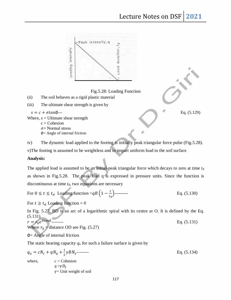
Lecture Notes on DSF 2021
117
Fig.5.28: Loading Function
(ii) The soil behaves as a rigid plastic material
(iii) The ultimate shear strength is given by
𝑠 = 𝑐 + 𝜎𝑡𝑎𝑛∅--- Eq. (5.129)
Where, s = Ultimate shear strength
c = Cohesion
𝜎= Normal stress ∅= Angle of internal friction
iv) The dynamic load applied to the footing is initially peak triangular force pulse (Fig.5.28).
v)The footing is assumed to be weightless and to impart uniform load to the soil surface
Analysis:
The applied load is assumed to be an initial-peak triangular force which decays to zero at time td
as shown in Fig.5.28. The peak load q is expressed in pressure units. Since the function is
discontinuous at time td, two equations are necessary
For 0 ≤ 𝑡 ≤ 𝑡𝑑 Loading function =𝑞𝐵 (1 −𝑡
𝑡𝑑)--------- Eq. (5.130)
For 𝑡 ≥ 𝑡𝑑 Loading function = 0
In Fig. 5.27, BD is an arc of a logarithmic spiral with its centre at O. It is defined by the Eq.
(5.131).
𝑟 = 𝑟0𝑒𝜃𝑡𝑎𝑛∅-------- Eq. (5.131)
Where 𝑟0 = distance OD see Fig. (5.27)
∅= Angle of internal friction
The static bearing capacity qu for such a failure surface is given by
𝑞𝑢 = 𝑐𝑁𝑐 + 𝑞𝑁𝑞 +1
2𝛾𝐵𝑁𝛾-------- Eq. (5.134)
where, c = Cohesion
q =𝛾𝐷𝑓
𝛾= Unit weight of soil

Lecture Notes on DSF 2021
118
𝐷𝑓 = Depth of footing
𝑁𝑐 , 𝑁𝑞 , 𝑁𝛾 = Bearing capacity factors
The bearing capacity factors depend on∅ and K, K being 2 (Distance OA)/H, Fig. 5.27. The
value of K locates the centre of the spiral which is the centre of rotation. Obviously the correct
value of K is that which yields the minimum value of the bearing capacity. It is obtained by trial
and error for each set of problem parameters. The values of 𝑁𝑐 , 𝑁𝑞 , 𝑁𝛾for various values of ∅ and
K are given in Column 3, 4 and 5 of Table 5.2.
Any acceleration of the soil mass ACDBA due to the downward movement of the footing will
cause inertial forces which will resist such movement. The inertial forces are directly
proportional to the acceleration of each individual soil mass and thereby dependent on
displacements. The effective total inertial force is obtained by combining the inertial forces on
each separate mass using energy considerations.
The inertial force is given by 𝐼𝑓 = 𝑁𝐼𝛾𝐵𝑑2∆
𝑑𝑡2------------ Eq. (5.135)
Where, ∆= Displacement at any time t
𝑁𝐼=Coefficient of dynamic inertial shear resistance.
The coefficient 𝑁𝐼 depends on ∅ and K, and its values are listed in column no. 6 of Table 5.2
Displacement of the soil mass within the failure surface due to downward movement of the
footing will increase the restoring moment about the point 0, and the increase in moment will be
proportional to the displacement provided the rotation is not excessive. It is expressed as
𝑅𝐹 = 𝑁𝑅𝐵𝛾∆--------- Eq. (5.136)
The coefficient NR also depends on ∅and K. Its values are listed in column no. 7 of Table 5.2.
The differential equations are established by equating the four vertical forces to zero. There must
be separate equations for before and after time td
For 0 ≤ 𝑡 ≤ 𝑡𝑑
𝑁𝐼𝛾𝐵𝑑2∆
𝑑𝑡2+ 𝑁𝑅𝛾𝐵∆ + 𝑞𝑢𝐵 − 𝑞𝐵 (1 −
𝑡
𝑡𝑑) = 0------- Eq. (5.137)
Or
For 𝑡 ≥ 𝑡𝑑
𝑁𝐼𝛾𝐵𝑑2∆
𝑑𝑡2+ 𝑁𝑅𝛾𝐵∆ + 𝑞𝑢𝐵 = 0----------- Eq. (5.138)
Or, 𝑑2∆
𝑑𝑡2+
𝑁𝑅
𝑁𝐼𝐵∆= −
𝑞𝑢
𝑁𝐼𝛾𝐵 ------------------ Eq. (5.139)
The solution of the differential equations will yield equations of footing displacement versus
time. The forms of the particular solutions of Eq. 5.140 are found to be
∆= 𝐶1 cos(𝐾,𝑡) + 𝐶2 sin(𝐾
,𝑡) + (𝑞−𝑞𝑢
𝑁𝑅𝛾) − (
𝑞
𝑁𝑅𝛾𝑡𝑑) 𝑡---------- Eq. (5.140)
And ∆= 𝐶3 cos(𝐾,𝑡) + 𝐶4 sin(𝐾
,𝑡) − (𝑞𝑢
𝑁𝑅𝛾)--------- Eq. (5.141)
In which 𝐾′ = √2𝑁𝑅
𝑁𝐼𝑅 and 𝐶1, 𝐶2, 𝐶3𝑎𝑛𝑑𝐶4 are coefficient of integration. The C1, C2 are evaluated
by the initial conditions. The coefficients C3 and C4 are obtained by conditions of displacement

Lecture Notes on DSF 2021
119
and velocity at td as defined by Eq. (5.140). After finding the solution and substitution of the
coefficients yield non-dimensional Eqs. 5.140 & 141 as
For 0 ≤ 𝑡 ≤ 𝑡𝑑
(𝑁𝑅𝛾
𝑞𝑢) ∆= (
𝑞
𝑞𝑢− 1) [1 − cos(𝐾′𝑡)] +
𝑞
𝑞𝑢
𝑡𝑑𝐾′[sin(𝐾′𝑡) − 𝐾′𝑡]---------- Eq. (5.142)
For 𝑡 ≥ 𝑡𝑑
(𝑁𝑅𝛾
𝑞𝑢)∆= [(1 −
𝑞
𝑞𝑢) +
𝑞
𝑞𝑢
𝑡𝑑𝐾′𝑠𝑖𝑛(𝐾′𝑡𝑑)] cos(𝐾
′𝑡𝑑) + [
𝑞
𝑞𝑢
𝑡𝑑𝐾′(1 − cos(𝐾′𝑡𝑑))] sin(𝐾
′𝑡𝑑) − − −−−Eq. (5.143)
The coefficients 𝑁𝛾 , 𝑁𝑐 , 𝑁𝑞, 𝑁𝐼𝑎𝑛𝑑𝑁𝑅 are dependent only on values of ∅ and K. Using
magnitudes of ∅ from 0° to 45° and of K for the region where the ultimate static shear resistance
could be a minimum, these coefficients were evaluated. The values obtained are given, in Table
5.2 for every fifth degree. The maximum displacement from Eq. 5.142 and 5.143 is the
predicated permanent footing displacement, since downward motion ceases at the time of the
maximum displacement.

Lecture Notes on DSF 2021
120
Fig. 5.29: Non-dimensional maximum displacement
Table 5.2: Bearing Capacity Factors
Φ(dgree) K 𝑁𝛾 𝑁𝑐 𝑁𝑞 𝑁𝐼 𝑁𝑅
√𝑁𝑅𝑁𝐼
0 -0.05 0.000 5.7277 1.00 0.0633 2.0125 5.6366
0.00 0.000 5.7124 1.00 0.0631 1.9723 5.5887
+0.05 0.000 5.7258 1.00 0.0633 1.9433 5.5394
5
-0.65 0.0454 79.6255 7,9664 0.03755 8.9076 4.8709
-0.60 0.1445 29.8163 3.6986 0.2280 6.4362 5.3126
-0.55 0.1481 18.9958 2.6619 0.1579 5.0332 5.6460
-0.50 0.1553 14.3469 2.2552 0.1213 4.1699 5.8636
-0.45 0.1655 11.8179 2.0339 0.1011 3.6088 5.9750
-0.40 0.1786 10.2699 1.8985 0.0897 3.2299 6.0020
-0.35 0.1945 9.2580 1.8100 0.0833 2.9674 5.9698
-0.30 0.2131 8.5723 1.7500 0.0799 2.7828 5.9005
-0.25 0.2344 8.1007 1.7087 0.0786 2.6523 5.8108
-0.20 0.2585 7.7778 1.6805 0.0785 2.5604 5.7116
-0.15 0.2855 7.5629 1.6617 0.0793 2.4969 5.6099
-0.10 0.3154 7.4291 1.6500 0.0809 2.4547 5.5096
-0.05 0.3483 7.3580 1.6437 0.0829 0.4288 5.4128
0.00 0.3843 7.3366 1.6419 0.0853 2.4155 5.3205
0.05 0.4233 7.3553 1.6435 0.0881 2.4122 5.2330
10
-0.60 0.5700 53.9491 10.5127 0.1120 5.7922 7.1922
-0.55 0.5588 28.9945 6.1125 0.0935 4.8411 7.1948
-0.50 0.5645 20.5266 4.6194 0.0833 4.2238 7.1228
-0.45 0.5832 16.3539 3.8837 0.0779 3.8095 6.9932
-0.40 0.6127 13.9337 3.4569 0.0757 3.5264 6.8293
-0.35 0.6521 12.4031 3.1870 0.0755 3.3323 6.6445
-0.30 0.7008 11.3881 3.0080 0.0767 3.2008 6.4587
-0.25 0.7586 10.7004 2.8868 0.0790 3.1147 6.2781
-0.20 0.8253 10.2345 2.8046 0.0821 3.0625 6.1071
-0.15 0.9012 9.9267 2.7503 0.0858 3.0360 5.9474
-0.10 0.9863 9.7361 2.7167 0.0901 3.0294 5.7994
-0.05 1.0807 9.6352 2.6990 0.0948 3.0386 5.6676
0.00 1.1848 9.6049 2.6936 0.0999 3.0604 5.5360
+0.05 1.2986 9.6313 2.6983 0.1053 3.0923 3.4187
15
-0.55 1.5462 46.5473 13.4724 0.0707 5.2677 8.6324
-0.50 1.5198 30.2759 9.1124 0.0696 4.7177 8.2310
-0.45 1.5342 23.2038 7.2175 0.0707 4.3564 7.8481
-0.40 1.5806 19.3483 6.1844 0.0734 4.1189 7.4903
-0.35 1.6540 16.9964 5.5542 0.0773 3.9669 7.1622
-0.30 1.7520 15.4722 5.1458 0.0823 3.8766 6.8645
-0.25 1.8730 14.4550 4.8732 0.0881 3.8322 6.5961
-0.20 2.0166 13.7730 4.6905 0.0947 3.8232 6.3542
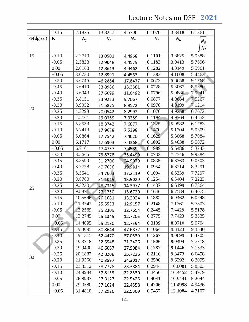
Lecture Notes on DSF 2021
121
-0.15 2.1825 13.3257 4.5706 0.1020 3.8418 6.1361
Φ(dgree) K 𝑁𝛾 𝑁𝑐 𝑁𝑞 𝑁𝐼 𝑁𝑅
√𝑁𝑅𝑁𝐼
15 -0.10 2.3710 13.0501 4.4968 0.1101 3.8825 5.9388
-0.05 2.5823 12.9048 4.4579 0.1183 3.9413 5.7596
0.00 2.8168 12.8613 4.4462 0.1282 4.0149 5.5961
+0.05 3.0750 12.8991 4.4563 0.1383 4.1008 5.4463
20
-0.50 3.6745 46.2884 17.8477 0.0673 5.6658 9.1768
-0.45 3.6419 33.8986 13.3381 0.0728 5.3067 8.5380
-0.40 3.6943 27.6099 11.0492 0.0796 5.0886 7.9941
-0.35 3.8151 23.9213 9.7067 0.0877 4.9684 7.5267
-0.30 3.9952 21.5875 8.8572 0.0970 4.9199 7.1214
-0.25 4.2298 20.0542 8.2992 0.1076 4.9258 6.7672
-0.20 4.5161 19.0369 7.9289 0.1194 4.9764 6.4552
-0.15 5.8533 18.3742 7.6877 0.1325 5.0582 6.1783
-0.10 5.2413 17.9678 7.5398 0.1470 5.1704 5.9309
-0.05 5.0864 17.7542 7.4620 0.1629 5.3068 5.7084
0.00 6.1717 17.6903 7.4368 0.1802 5.4638 5.5072
+0.05 6.7161 17.4757 7.4589 0.1989 5.6486 5.3243
25
-0.50 8.5665 73.8778 35.4499 0.0732 7.2346 9.9384
-0.45 8.3599 51.2706 24.9079 0.0835 6.8363 9.0503
-0.40 8.3728 40.7056 19.9814 0.0954 6.6214 8.3291
-0.35 8.5541 34.7663 17.2119 0.1094 6.5339 7.7297
-0.30 8.8760 31.1015 15.5029 0.1254 6.5404 7.2223
-0.25 9.3230 28.7315 14.3977 0.1437 6.6199 6.7864
-0.20 9.8871 27.1750 13.6720 0.1646 6.7584 6.4075
-0.15 10.5646 26.1681 13.2024 0.1882 6.9462 6.0748
-0.10 11.3542 25.5533 12.9157 0.2148 7.1761 5.7803
-0.05 12.2569 25.2309 12.7654 0.2445 7.4429 5.5178
0.00 13.2745 25.1345 12.7205 0.2775 7.7423 5.2825
+0.05 14.4095 25.2180 12.7594 0.3139 8.0710 5.0704
30
-0.45 19.3095 80.8644 47.6872 0.1064 9.3123 9.3540
-0.40 19.1315 62.4470 37.0539 0.1267 9.0899 8.4705
-0.35 19.3718 52.5548 31.3426 0.1506 9.0494 7.7518
-0.30 19.9400 46.6067 27.9084 0.1787 9.1446 7.1533
-0.25 20.1887 42.8208 25.7226 0.2116 9.3473 6.6458
-0.20 21.9566 40.3597 24.3017 0.2500 9.6392 6.2095
-0.15 23.3512 38.7778 23.3884 0.2944 10.0081 5.8303
-0.10 24.9984 37.8159 22.8330 0.3456 10.4452 5.4979
-0.05 26.8993 37.3127 22.5425 0.4041 10.9441 5.2044
0.00 29.0580 37.1624 22.4558 0.4706 11.4998 4.9436
+0.05 31.4810 37.2926 22.5309 0.5457 12.1084 4.7107

Lecture Notes on DSF 2021
122
35 -0.45 46.2942 134.3023 95.0397 0.1527 13.4981 9.4021
Φ(dgree) K 𝑁𝛾 𝑁𝑐 𝑁𝑞 𝑁𝐼 𝑁𝑅
√𝑁𝑅𝑁𝐼
35
-0.40 45.4427 100.66099 71.4837 0.1887 13.2639 8.3844
-0.35 45.6687 83.4477 59.4308 0.2323 13.3114 7.5703
-0.30 46.7356 73.3676 52.3727 0.2849 13.5708 6.9017
-0.25 48.5145 67.0529 47.9511 0.3481 14.0015 6.3419
-0.20 50.9356 62.9887 45.1052 0.4237 14.5786 5.8661
-0.15 53.9640 60.3926 43.2874 0.5133 15.2895 5.4569
-0.10 57.8568 58.8199 42.1864 0.6191 16.1127 5.1018
-0.05 61.8051 57.9989 41.6113 0.7428 17.0515 4.7911
0.00 66.6196 57.7539 41.4398 0.8868 18.0970 4.5175
+0.05 72.0773 57.9662 41.5884 1.0526 19.2451 4.2753
40
-0.40 115.7097 172.8231 146.0161 0.3229 20.8738 8.0404
-0.35 115.5504 141.1002 119.3973 0.4107 21.1138 7.1701
-0.30 117.6386 123.0124 104.2199 0.5195 21.7125 6.4650
-0.25 121.5875 111.8576 94.8599 0.6536 22.6077 5.8817
-0.20 127.1879 104.7472 88.8935 0.8175 23.7619 5.3914
-0.15 134.3346 100.2323 85.1051 1.0168 25.1570 4.9741
-0.10 142.9868 97.5069 82.8181 1.2572 26.7775 4.6152
-0.05 153.1451 96.0866 81.6263 1.5450 28.6173 4.3038
0.00 164.839 95.6630 81.2709 1.8870 30.6724 4.0317
+0.05 178.1176 96.0303 81.5791 2.2904 32.9409 3.7924
45
-0.40 327.6781 322.2748 323.2752 0.6576 36.2961 7.4295
-0.35 325.4943 259.1345 260.1349 0.8611 37.0113 6.5559
-0.30 329.9752 224.0769 225.0772 1.1194 38.3965 5.8568
-0.25 339.8627 202.7837 203.7840 1.4447 40.3468 5.2846
-0.20 354.4804 189.3358 190.3361 1.8515 42.8070 4.8083
-0.15 373.4971 180.8450 181.8452 2.3565 45.7496 4.4062
-0.10 393.7473 175.7358 176.7361 2.9784 49.1634 4.0628
-0.05 424.2605 173.0775 174.0778 3.7386 53.0475 3.7669
0.00 456.1177 172.2851 173.2853 4.6607 57.4067 3.5096
+0.05 492.4763 172.9729 173.9732 5.7709 62.2499 3.2843

Lecture Notes on DSF 2021
123
5.11 Seismic Bearing Capacity and Settlement in Granular Soil
The shallow foundations may fail during seismic events. Published studies relating to the
bearing capacity of shallow foundations in such instances are rare. In 1993, however,
Richards et al. developed a seismic bearing capacity theory to find seismic bearing capacity
of granular soil. Figure 5.30 shows a failure surface in soil assumed for the subsequent
analysis, under static conditions. Similarly, Figure 5.31 shows the assumed failure under
earthquake conditions. Note that, in the two figures,
𝛼𝐴,𝛼𝐴𝐸 = inclination angles for active pressure conditions
And
𝛼𝑃,𝛼𝑃𝐸= inclination angles for passive pressure conditions
Fig.5.30: Assumed failure surface in soil for static bearing capacity analysis
Fig.5.31: Assumed failure surface in soil for seismic bearing capacity analysis
According to this theory, the ultimate bearing capacities for continuous foundations in
granular soil are
𝑞𝑢 = 𝑞𝑁𝑞 +1
2𝛾𝐵𝑁𝛾, For static condition--------------------- Eq. (5.144)
𝑞𝑢𝐸 = 𝑞𝑁𝑞𝐸 +1
2𝛾𝐵𝑁𝛾𝐸, For Earthquake conditions------------ Eq. (5.145)
Where, 𝑁𝑞, 𝑁𝛾, 𝑁𝑞𝐸, 𝑁𝛾𝐸 are bearing capacity factors

Lecture Notes on DSF 2021
124
Again, 𝑁𝑞, 𝑁𝛾 = 𝑓(∅′)
And 𝑁𝑞𝐸, 𝑁𝛾𝐸 = 𝑓(∅′, 𝑡𝑎𝑛𝜃)
Where 𝑡𝑎𝑛𝜃 =𝑘ℎ
1−𝑘𝑣---------------- Eq. (5.146)
𝑘ℎ= Horizontal coefficient of earthquake acceleration
𝑘𝑣= Vertical coefficient of earthquake acceleration
Using the failure surface shown in Figure 5.31, Richards, Elms and Budhu (1993) provided
the values of bearing capacity factors, 𝑁𝑞, and 𝑁𝛾,. They are given in Table 5.3
Table 5.3: Bearing capacity factors
The variations of 𝑁𝑞 and 𝑁𝛾 with ∅′ are shown in Figure 5.32. Figure 5.33 shows the variations
of 𝑁𝛾𝐸
𝑁𝛾⁄ and
𝑁𝑞𝐸𝑁𝑞
⁄ with 𝑡𝑎𝑛𝜃 and the soil angle ∅′based on this analysis.
Fig. 5.32: Variation of 𝑁𝑞 and 𝑁𝛾 based on failure surface assumed in Figure 5.30

Lecture Notes on DSF 2021
125
Fig. 5.33: Variation of𝑁𝛾𝐸
𝑁𝛾⁄ and
𝑁𝑞𝐸𝑁𝑞
⁄ with 𝑡𝑎𝑛𝜃
Under static conditions, bearing capacity failure can lead to a substantial sudden downward
movement of the foundation. However, bearing capacity related settlement in an earthquake is
important and it takes place when the ratio 𝑡𝑎𝑛𝜃 =𝑘ℎ
(1 − 𝑘𝑣)⁄ reaches the critical value. The
critical value can be expressed as [𝑘ℎ
(1−𝑘𝑣)] 𝑐𝑟𝑖𝑡𝑖𝑐𝑎𝑙 becomes equal to 𝑘ℎ
∗ when 𝑘𝑣=0
Table 5.4: Variation of 𝛼𝐴𝐸 with 𝑘ℎ∗ and soil friction angle ∅′
Figure 5.34 shows the variation of 𝑘ℎ
∗ (for 𝑘𝑣 = 0 ) with the factor of safety (FS) applied to the
ultimate static bearing capacity [Eq. 5.144], with ∅′ , and with 𝐷𝑓
𝐵⁄ (for ∅′ = 300 and 400 ).

Lecture Notes on DSF 2021
126
Fig.5.34: Critical acceleration 𝑘ℎ
∗ for 𝑘𝑣=0
The settlement of a strip foundation due to an earthquake using a sliding block approach can be
estimated (Richards, Elms and Budhu, 1993) as
𝑆𝐸𝑞(𝑚) = 0.174𝑉2
𝐴𝑔[𝑘ℎ∗
𝐴]−4
𝑡𝑎𝑛𝛼𝐴𝐸---------------------- Eq. (5.147)
Where, V = peak velocity for the design earthquake (m/sec)
A = acceleration coefficient for the design earthquake
g = acceleration due to gravity (9.81 m/s2)
The values of 𝑘ℎ∗ and 𝛼𝐴𝐸 can be obtained from Figure 5.34 and Table 5.4, respectively. This
approach can be used to design a footing based on limiting seismic settlements.
Problem No.1
A rectangular foundation has a length L of 2.5 m. It is supported by medium dense sand with a
unit weight of 17 kN/m3. The sand has an angle of friction of 36º. The foundation may be
subjected to a dynamic load of 735 kN increasing at a moderated rate. Using a factor of safety
equal to 2, determine the width of the foundation. Use Df = 0.8 m.
APPENDIX (Foundation for Various Types Machines)

Lecture Notes on DSF 2021
127
DESIGN OF RECIPROCATING MACHINE FOUNDATION
Reciprocating Machine should be placed over suitable Vibration Absorber to reduce the
magnitude of displacement due to dynamic unbalanced force produced due the Machine.
Design for Vibration absorber: The following steps are required
1 Make a trial design without absorber
2 Depending on requirement of minimum foundation size, for the machine selection of
block foundation size is made.
3 Determine stiffness due to vertical vibration Kz=K1
4 Determine the natural frequency of soil, considering total mass due to machine and
foundation, 𝑤𝑛𝑙1=√𝐾1
𝑚1+𝑚2
5 Find mass ratio n =𝑚2
𝑚1
6 Determine frequency ratio a1=𝑤𝑛𝑙1
𝑤, w is the operating frequency
7 Compute displacement magnitude without absorber as , Zmax
Zmax=𝐹0
(𝑚1+𝑚2)(𝑤𝑛𝑙12 −𝑤2)
8 Calculate efficiency of absorber η=𝑍1
𝑍𝑚𝑎𝑥, z1is the permissible displacement
9 Again efficiency can be expressed as
η=𝑎22(1+𝑛)(𝑎1
2−1)
[1−(1+𝑛)(𝑎12+𝑎2
2−𝑎12𝑎2
2)] where a2 is the frequency ratio, 𝑎2 =
𝑤𝑛𝑙2
𝑤
wnl2 is the natural frequency of absorber.
10 Find stiffness of absorber K2=𝑚2𝑤𝑛𝑙22
11 Suitable absorber may be selected from K2
12 Find Z2=[(1+𝑛)𝑎1
2+𝑛𝑎22−1]𝐹0
𝑚2𝜔2[1−(1+𝑛)(𝑎1
2+𝑎22−𝑎1
2𝑎22)]
, Than check for maximum force of resistance
13 Find magnitude of force resistance𝐹0 = 𝐾2𝑍2
Q.1 Determine the stiffness of the absorber to be kept between a reciprocating machine and
foundation to bring the vibration amplitude to less than 0.02 mm. The weight of the machine is
18 kN. It produces an unbalanced force of 4 kN, when operated at speed of 600rpm. Shear
modulus of foundation soil G=20MN/m2 and µ= 0.35.
Sol: Mass of the block foundation of dimension 4x3m2 with 1.5 m height
𝑚1 =24×4×3×1.5
9.81= 44kg

Lecture Notes on DSF 2021
128
Mass of machine 𝑚2 =18
9.81= 1.83kg,
Equivalent radius of circular footing 𝑟 = √4×3
𝜋=1.95 m
Stiffness in vertical direction, 𝐾𝑧 =4𝐺𝑟
1−µ=240000 kN/m
Natural frequency of vibration, 𝜔𝑛𝑙1 = √240000
44+1.83=72.36 r/sec
Operating frequency of machine, 𝜔 =2𝜋×600
60= 62.83 r/sec
Maximum amplitude of vertical vibration (Without absorber)
𝑍𝑚𝑎𝑥 =𝐹0
(𝑚1+𝑚2)(𝜔𝑛𝑙12 −𝜔2)
=0.068 mm
Efficiency of absorber= 𝑍1
𝑍𝑚𝑎𝑥=0.02
0.068=0.333
Frequency ratio, 𝑎1 =𝜔𝑛𝑙1
𝑤=1.15, Mass ratio, 𝜂 =
𝑚1
𝑚2=0.0415
Now efficiency can also be expressed as η=𝑎22(1+𝑛)(𝑎1
2−1)
[1−(1+𝑛)(𝑎12+𝑎2
2−𝑎12𝑎2
2)]
Hence, 0.333=𝑎22(1+0.0415)(1.152−1)
[1−(1+0.0415)(1.152+𝑎22−1.152𝑎2
2)]
So 𝑎2=1.31
But 𝑎2 =𝜔𝑛𝑙2
𝜔, hence 𝜔𝑛𝑙2=81.97 r/s
Z2=[(1+𝑛)𝑎1
2+𝑛𝑎22−1]𝐹0
𝑚2𝜔2[1−(1+𝑛)(𝑎1
2+𝑎22−𝑎1
2𝑎22)]
= [(1+0.0415)1.152+0.0415×1.312−1]×4
1.83×62.832[1−(1+0.0415)(1.152+1.312−1.152×1.312)]= −58.47mm
Resisting force of absorber 𝐹0 = 𝐾2𝑍2=12298x0.05847=719 kN
MACHINE FOUNDATION ON PILES
Piles divided into two groups: End bearing and Friction Piles
Longitudinal Vibration of Short Elastic Bar:

Lecture Notes on DSF 2021
129
i) End Bearing Pile: Mass of Pile is negligible
Wave equation: 𝜕2𝑢
𝜕𝑡2=𝑣𝑐
2 𝜕2𝑢
𝜕𝑥2-------- Eq.(1)
Where u is the displacement function and vc is shear wave velocity
Solution to above second order differential equation is expressed as
u(x,t)=U(x)(A1sinωnt+A2cosωnt)--- Eq.(2)
Where A1 and A2 are two constants, ωn is the natural frequency and U(x) is amplitude of
displacement along the length of the bar and is independent of time “t”
Eq. 1 can be rewritten by putting value from Eq.2 as
𝜕2𝑈(𝑥)
𝜕𝑥2+
𝜌
𝐸𝜔𝑛2𝑈(𝑥) = 0----- Eq.(3)
Now general solution to the above Eq.3 can be given as
U(x) =𝐵1sin(𝜔𝑛𝑥
𝑣𝑐) +𝐵2cos(
𝜔𝑛𝑥
𝑣𝑐)----- Eq. (4)
Using end conditions a) Fixed
At x=0, U(x) =0 which gives B2=0
At x=L, 𝑑𝑈(𝑥)
𝑑𝑥= 0, gives
𝐵1
𝑣𝑐𝜔𝑛𝑐𝑜𝑠
𝜔𝑛𝐿
𝑣𝑆=0,
Hence, 𝑐𝑜𝑠𝜔𝑛𝐿
𝑣𝑐= 0, or
𝜔𝑛𝐿
𝑣𝑐=
(2𝑛−1)𝜋
2
Which gives, 𝜔𝑛 =1
2(2𝑛 − 1)𝜋
𝑣𝑐
𝐿, for n=1 𝜔𝑛 =
𝜋
2
𝑣𝑐
𝐿
So natural frequency 𝑓𝑛 =𝜔𝑛
2𝜋=1
4𝐿√𝐸𝑝
𝜌𝑝--------------- Eq.(5)
Where Ep and 𝜌P are Young’s modulus and density of pile material
Now mass of pie is considered as “m”
The general solution is again taken as U(x) =𝐵1sin(𝜔𝑛𝑥
𝑣𝑐) +𝐵2cos(
𝜔𝑛𝑥
𝑣𝑐)
From end condition, we get B2=0 which gives U(x) =𝐵1sin(𝜔𝑛𝑥
𝑣𝑐)
At x=L, the inertia force of mass m is acting on the soil column and this can be expressed as
𝐹 = −𝑚𝜕2𝑢
𝜕𝑡2------------------ Eq.(6)
Strain in the pile is expressed as 𝜖=𝜕𝑢
𝜕𝑥=
𝐹
𝐴𝐸------------ Eq.(7)
Where E and A are Young’s modulus and area of cross section of pile respectively. 𝐹
𝐴𝐸=
𝜕𝑢
𝜕𝑥=
𝜕𝑈
𝜕𝑥(𝐴1𝑠𝑖𝑛𝜔𝑛𝑡 + 𝐴2𝑐𝑜𝑠𝜔𝑛𝑡)-------- Eq.(8)
Substituting for, 𝜕𝑈
𝜕𝑥 , above Expression becomes
𝐵1𝜔𝑛
𝑣𝑐cos (
𝜔𝑛𝑥
𝑣𝑐) (𝐴1𝑠𝑖𝑛𝜔𝑛𝑡 + 𝐴2𝑐𝑜𝑠𝜔𝑛𝑡) =
𝐹
𝐴𝐸------- Eq.(9)
Now, 𝐹 = −𝑚𝜕2𝑢
𝜕𝑡2= −𝑚[𝐵1sin(
𝜔𝑛𝑥
𝑣𝑐)]
𝜕2
𝜕𝑡2(𝐴1𝑠𝑖𝑛𝜔𝑛𝑡 + 𝐴2𝑐𝑜𝑠𝜔𝑛𝑡)------ Eq.(10)
Or, 𝐹 = 𝑚𝜔𝑛2𝐵1sin(
𝜔𝑛𝑥
𝑣𝑐)(𝐴1𝑠𝑖𝑛𝜔𝑛𝑡 + 𝐴2𝑐𝑜𝑠𝜔𝑛𝑡)----------- Eq.(11)
From Eq.(9) and (10), we get 𝐴𝐸
𝑣𝑐cos (
𝜔𝑛𝑥
𝑣𝑐) = 𝑚𝜔𝑛sin(
𝜔𝑛𝑥
𝑣𝑐)------ Eq.(12)
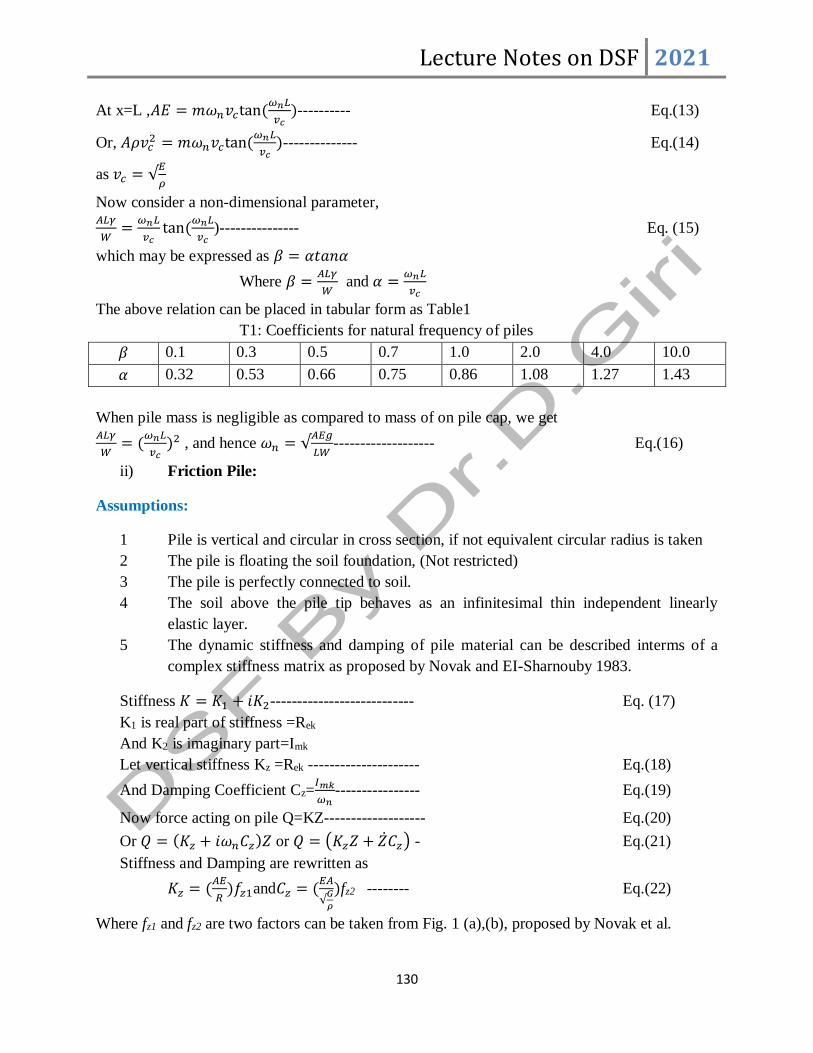
Lecture Notes on DSF 2021
130
At x=L ,𝐴𝐸 = 𝑚𝜔𝑛𝑣𝑐tan(𝜔𝑛𝐿
𝑣𝑐)---------- Eq.(13)
Or, 𝐴𝜌𝑣𝑐2 = 𝑚𝜔𝑛𝑣𝑐tan(
𝜔𝑛𝐿
𝑣𝑐)-------------- Eq.(14)
as𝑣𝑐 = √𝐸
𝜌
Now consider a non-dimensional parameter, 𝐴𝐿𝛾
𝑊=
𝜔𝑛𝐿
𝑣𝑐tan(
𝜔𝑛𝐿
𝑣𝑐)--------------- Eq. (15)
which may be expressed as 𝛽 = 𝛼𝑡𝑎𝑛𝛼
Where 𝛽 =𝐴𝐿𝛾
𝑊 and 𝛼 =
𝜔𝑛𝐿
𝑣𝑐
The above relation can be placed in tabular form as Table1
T1: Coefficients for natural frequency of piles
𝛽 0.1 0.3 0.5 0.7 1.0 2.0 4.0 10.0
𝛼 0.32 0.53 0.66 0.75 0.86 1.08 1.27 1.43
When pile mass is negligible as compared to mass of on pile cap, we get 𝐴𝐿𝛾
𝑊= (
𝜔𝑛𝐿
𝑣𝑐)2 , and hence 𝜔𝑛 = √
𝐴𝐸𝑔
𝐿𝑊------------------- Eq.(16)
ii) Friction Pile:
Assumptions:
1 Pile is vertical and circular in cross section, if not equivalent circular radius is taken
2 The pile is floating the soil foundation, (Not restricted)
3 The pile is perfectly connected to soil.
4 The soil above the pile tip behaves as an infinitesimal thin independent linearly
elastic layer.
5 The dynamic stiffness and damping of pile material can be described interms of a
complex stiffness matrix as proposed by Novak and EI-Sharnouby 1983.
Stiffness 𝐾 = 𝐾1 + 𝑖𝐾2--------------------------- Eq. (17)
K1 is real part of stiffness =Rek
And K2 is imaginary part=Imk
Let vertical stiffness Kz =Rek --------------------- Eq.(18)
And Damping Coefficient Cz=𝐼𝑚𝑘
𝜔𝑛---------------- Eq.(19)
Now force acting on pile Q=KZ------------------- Eq.(20)
Or 𝑄 = (𝐾𝑧 + 𝑖𝜔𝑛𝐶𝑧)𝑍 or 𝑄 = (𝐾𝑧𝑍 + ��𝐶𝑧) - Eq.(21)
Stiffness and Damping are rewritten as
𝐾𝑧 = (𝐴𝐸
𝑅)𝑓𝑧1and𝐶𝑧 = (
𝐸𝐴
√𝐺
𝜌
)fz2 -------- Eq.(22)
Where fz1 and fz2 are two factors can be taken from Fig. 1 (a),(b), proposed by Novak et al.

Lecture Notes on DSF 2021
131
Fig. 1:Stiffness and Damping Parameters of Vertical Response for: a) End Bearing Piles and b)
Floating Piles (reprinted from Novak and El Sharnouby 1983, © ASCE)
Stiffness and Damping of Pile Group
𝐾𝑧(𝑔) =∑𝐾𝑧
∑𝛼𝑟and𝐶𝑧(𝑔) =
∑𝐶𝑧
∑𝛼𝑟 ---------------------- Eq.(23)
Where 𝛼𝑟= Interaction factor and is obtained from the table T:3.6 page 49 (Hand book of
Machine Foundation by Srinivasulu &Vaidyanatham)
S/D=Pile Spacing/Diameter of Pile 3.0 45 6.0 ∞
𝛼𝑟 0.35 0.58 0.63 1.0
Stiffness and Damping Coefficient of Pile Cap:
𝐾𝑧(𝑐𝑎𝑝) = 𝐺𝑠𝐷𝑓𝑆1--------------------------------------- Eq.(24)
𝐶𝑧(𝑐𝑎𝑝) = 𝐷𝑓𝑟0𝑆2√𝐺𝑠𝜌𝑠-------------------------------- Eq.(25)
Where r0 is the equivalent radius of pile cap and Df is the depth of pile cap from ground surface
S1 and S2 are constants and may be taken as 2.7 and 6.7 respectively.
Now total stiffness and Damping Coefficient can be obtained as
𝐾𝑧(𝑇) = 𝐾𝑧(𝑔) + 𝐾𝑧(𝑐𝑎𝑝)-------------------------------- Eq.(26)
𝐶𝑧(𝑇) = 𝐶𝑧(𝑔) + 𝐶𝑧(𝑐𝑎𝑝)-------------------------------- Eq.(27)
Damping Ratio in Vertical Direction
𝐷𝑧 =𝐶𝑧(𝑇)
2√𝐾𝑧(𝑇)𝑚 --------------------------------------------- Eq.(28)

Lecture Notes on DSF 2021
132
𝜔𝑛 = √𝐾𝑧(𝑇)
𝑚------------------------------------------------ Eq.(29)
Amplitude of Displacement: For constant force of excitation
𝐴𝑧 =𝑄0
𝐾𝑧
1
𝐷𝑧√(1−𝐷𝑧2 )
--------------------------------------- Eq.(30)
Amplitude of Displacement: For rotating mass type of excitation
𝐴𝑧 =𝑚𝑒𝑒
𝑀
1
𝐷𝑧√(1−𝐷𝑧2)
--------------------------------------- Eq.(31)
Q.1 A group of four piles having dimension 0.3x0.3 m2 is supported a machine foundation as
shown in Fig. Determine total stiffness and damping coefficient, given Ep=2.1x10⁷ kN/m2, unit
weight of soil18.9 kN/m2, Poisson’s ratio 0.5 and shear modulus Gs=28120 kN/m2.
Solution: Equivalent radius of pile cap r0=√(1.5𝑋0.6)2
𝜋= 1.18 m
1.5m
12m
2.0 m
1.5 m
2.1 m
B
C D
A
GL

Lecture Notes on DSF 2021
133
Equivalent radius of pile R= √(0.3𝑋0.3)2
𝜋= 0.17 m
Vertical stiffness of pile, 𝐾𝑧 = (𝐴𝐸
𝑅)𝑓𝑧1=
2.1𝑥107×0.32
0.17× 𝑓𝑧1, 𝑓𝑧1is found from Fig 1(b) as 0.035
= 389.1x10³kN/m2
NowE
G=
2.1×10⁷
28120= 746.8= say 750
𝐿
𝑅=
12
0.17=70.58, From Fig. 1(b)𝑓𝑧2=0.06
Hence Damping Coefficient is calculated as 𝐶𝑧 = (𝐸𝐴
√𝐺
𝜌
)fz2 =2.1×107×0.32
√28120×9.81
18.9
x0.06=938.7 kN.s/m
Calculation of Interaction factor:
𝑆
𝐷=1.5
0.34=4.41 for pile A to B, A to D
A A B C D
1 0.54 0.48 0.54
B 0.54 1.0 0.54 0.48
C 0.48 0.54 1.0 0.54
D 0.54 0.48 0.54 10
∑αr 2.56 2.56 2.56 2.56
If the sum of interaction factors is not same, than take average value of ∑𝛼𝑟
Kzr(g)=∑𝐾𝑧
∑𝛼𝑟=4×389100
2.56=607968.75kN/m
𝐶𝑍(𝑔) =∑𝐶𝑧
∑𝛼𝑟=1446.78 kNs/m
Now Stiffness and Damping Coefficient for Pile Cap
𝐾𝑧(𝑐𝑎𝑝) = 𝐺𝑠𝐷𝑓𝑆1 = 28120 × 1.5 × 2.7 = 113886𝑘𝑁/𝑚
And Damping Coefficient for Pile Cap
𝐶𝑧(𝑐𝑎𝑝) = 𝐷𝑓𝑟0𝑆2√𝐺𝑠𝜌𝑠=2720 kNs/m
Now total Stiffness and Damping Coefficient are calculated as
𝐾𝑧(𝑇) = 𝐾𝑧(𝑔) + 𝐾𝑍(𝑐𝑎𝑝)=607968.75+113886=721854.75 kN/m
𝐶𝑧(𝑇) = 𝐶𝑧(𝑔) + 𝐶𝑍(𝑐𝑎𝑝)=1446.78+2720=4166.78 kNs/m
Problem 1 A machine is supported by four pre-stressed concrete piles driven into a bed rock.
The length of each pile is 8o ft long and is 12x12 in2 in cross section. The weight of the machine
and foundation is 300x103lbs, unit weight 150 lb/ft3. The Young’s modulus is 3.5x10⁶lb/in2.
Determine the natural frequency of pile foundation system.
FRAMED FOUNDATION FOR MACHINE
Lecture Notes on DSF 2021
134
In the case of a frame foundation, it is necessary to check the frequencies and amplitudes of
vibration and also to design the members of frame from structural considerations. The methods
for carrying out dynamic analysis may be divided into two categories:
(a) Two-.dimensional analysis
(b) Three-dimensional analysis
The two-dimensional analysis (Also known as Simplified Method) is based on the following
assumptions:
Each transverse frame that consists of two columns and a beam perpendicular to the main shaft
of the machine is considered separately. The stiffness of the equivalent spring is calculated as the
combined stiffness of the beam and the column acting together and the mass is determined by the
mass of total loads acting on the cross frame.
Following Assumptions are made.
i) Frame columns are fixed at their lower ends into the rigid base slabs.
ii) The difference in vertical deformation of individual frame column is neglected
iii) Torsional resistance of longitudinal beam is insignificant compare to the deformation
resistance of transverse beam. Therefore, the effect of longitudinal beam on vertical
vibration of transverse frame can be neglected.
iv) The natural frequencies of individual cross frame are practically of same order.
v) The effect of elasticity of soil is neglected.
vi) The connection of transverse beam with column is also neglected.
Determination of Vertical Frequency:
For obtaining vertical frequency, each transverse frame that consists of two columns and a beam
perpendicular to main shaft of the machine is considered separately as shown in Fig. 1

Lecture Notes on DSF 2021
135
Fig. 1 a) Typical Transverse Frame b) Idealised Model
The loads acting on this frame are
(I) Dead load of the machine and bearing, Wm
(ii) Load transferred to the columns by longitudinal beams, W1
(iii) Uniformly distributed load due to self weight of cross beam, q per unit length
(Iv) Unbalanced vertical force due to machine operation, 𝐹𝑧sin(𝜔𝑡)
The mass-spring system used as model for the frame is shown in Fig.1 (b). The stiffness of
equivalent spring (K) is computed as the combined stiffness of the beam and columns acting
together. It is given by
𝐾𝑧 =𝑊
𝛿𝑠𝑡------ Eq.1
Where W = Total load on the frame=Wm+2WL+qL
L= Effective span
𝛿𝑠𝑡= Total vertical deflection at the vcentre of the beam due to bending action of beam and axial
compression in column.
So, 𝛿𝑠𝑡 = 𝛿1 + 𝛿2 + 𝛿3 + 𝛿4-------- Eq.2
𝛿1=Vertical deflection of beam due to load Wm
𝛿2= Vertical deflection of beam due to distributed load q
𝛿3=Vertical deflection of beam due to shear
𝛿4=Axial compression in column
Now the magnitude of each deflection components can be obtained as

Lecture Notes on DSF 2021
136
𝛿1 =𝑊𝑚𝐿3
96𝐸𝐼𝑏
2𝐾+1
𝐾+2,
𝛿2 =𝑞𝐿4
384𝐸𝐼𝑏
5𝐾+2
𝐾+2
𝛿3 =3
5𝐸𝐴𝑏(𝑊𝑚 +
𝑞𝐿
2)
𝛿4 =ℎ
𝐸𝐴𝑐(𝑊𝐿 +
𝑊𝑚𝐿
2)
Where
𝐴𝑏=Cross sectional area of beam, 𝐴𝑐= Cross sectional area of column
𝐼𝑐=Moment of inertia of beam about the axis of bending
E= Young’s modulus of concrete, K=Relative stiffness factor=𝐼𝑏
𝐼𝑐×
ℎ
𝐿
L= Effective span of frame, h= Effective height of frame
The values of L and h are taken as
𝐿 = 𝑙0 − 2𝛼𝑏 , ℎ = ℎ0 − 2𝛼𝑎
l0 = Centre to centre distance between columns (Fig. 1a)
h0 = Height of the column from the top of the base slab to the centre of the frame beam (Fig. 1a)
a = One-half of the depth of the beam for a frame without haunches (Fig. 1a) or the distance as
shown in Fig. 2 for a frame with haunches
b = One-half of the column width for a frame without haunches (Fig. 1a) or the distance as
shown in Fig. 2 for a frame with haunches.
Knowing the values of ℎ0, 𝑙0 and b, α can be obtained from Fig. 3.
Fig. 2: values of a and b for a frame with haunches. Fig.3: α versus 𝑏
𝑙0

Lecture Notes on DSF 2021
137
The natural frequency of a transverse frame in vertical vibrations is given by
𝜔𝑛𝑧 = √𝐾𝑧𝑔
𝑊------- Eq.3
Average vertical natural frequency of the T. G. Foundation is taken as:
𝜔𝑛𝑧𝑎 =𝜔𝑛𝑧1+𝜔𝑛𝑧2+−−+𝜔𝑛𝑧𝑛
𝑛------- Eq.4
𝜔𝑛𝑧1 , 𝜔𝑛𝑧2,etc =Vertical frequencies of individual transverse frames
Vertical Vibration Amplitude:
𝐴𝑍 =𝑃𝑍
∑𝐾𝑍√(1−𝜔2
𝜔𝑛𝑧𝑎2 )2+(2𝐷
𝜔
𝜔𝑛𝑧𝑎)2
------------ Eq.5
𝐴𝑍=Average vertical amplitude of vibration og foundation
𝑃𝑍=Total vertical imbalance force
∑𝐾𝑍= Sum of the stiffness of the individual frames
𝜔𝑛𝑧𝑎= Average value of natural frequency
D= Damping ratio
For under-tuned foundation, i.e. 𝜔 < 𝜔𝑛𝑧 or 𝜔𝑛 = 𝜔𝑛𝑧𝑎
The maximum amplitude of vibration can be expressed as
𝐴𝑍(𝑚𝑎𝑥) =𝑃𝑍
∑𝐾𝑍×
1
2𝐷-------------- Eq.6
Horizontal Vibration Analysis:
The following assumptions are made during analysis of horizontal vibration of frame foundation
i) Columns are fixed into the rigid base slab at lower ends.
ii) The deck slab is rigid in its own plane.
iii) The resistance offered by the column in axial compression is large as compare to their
resistance in bending.
iv) Torsional vibration of deck slab is neglected.
v) Elastic resistance of the soil at the base can be neglected.
The spring stiffness is provided by the columns due to their bending action and for any
transverse frame is given by
𝐾𝑥𝑖 =12𝐸𝐼𝑐
ℎ3(6𝐾+1
3𝐾+2)---------- Eq.7
𝐾𝑥𝑖=Lateral stiffness of an individual transverse frame.
The natural frequency of frame foundation is given by

Lecture Notes on DSF 2021
138
𝜔𝑛𝑥𝑎 = √∑(𝐾𝑥)𝑔
𝑊𝑇 --------------- Eq.8
Where WT is the total weight of deck slab and machine
The average horizontal amplitude of vibration of the foundation may be expressed as
𝐴𝑥 =𝑃𝑥
∑𝐾𝑛𝑥√(1−𝜔2
𝜔𝑛𝑥2 )2+(2𝐷
𝜔
𝜔𝑛𝑥)2
-------- Eq.9
For under-tuned foundation, i.e. 𝜔 < 𝜔𝑛𝑧 or 𝜔𝑛 = 𝜔𝑛𝑧𝑎
The maximum amplitude of vibration can be expressed as
𝐴𝑥,𝑚𝑎𝑥 =𝑃𝑥
∑𝐾𝑥×
1
2𝐷-------- Eq.10
Two Degree of Freedom (Amplitude Method) Analysis:
Fig. 4(a) Section nof cross frame (b) Mathematical model
Vertical Vibration Analysis:
For the vertical frequency a two-degree-spring-mass system shown in Fig. 4(b) is adopted. Mass
m1 lumped over the columns is given as
𝑚1 =𝑊1+𝑊2+0.33𝑊3+0.25𝑊4
𝑔--------- Eq.11
Mass m2 acting at the centre of the cross beam is given as
𝑚1 =𝑊2+0.45𝑊4
𝑔--- Eq.12
𝑊1=Dead load of the machine and bearing
𝑊2= Load transferred to column by lognitudinal beams.
𝑊3=Weight of two columns contituting the transverse frame

Lecture Notes on DSF 2021
139
𝑊4=Weight of the tranverse beam
The stiffness K1 of both the column of a transverse frame is given by
𝐾1 =2𝐸𝐴𝑐
ℎ--------------- Eq.13
The stiffness K2 of the frame is given as
𝐾2 =1
∆𝑧---------- Eq.14
∆𝑧 =𝑙(1+2𝐾)
96𝐸𝐼𝑏(2+𝐾)+
3𝑙
8𝐺𝐴𝑏------- Eq.15
G = Shear modulus of beam material
E = Young's modulus of columns material
Ac = Cross-sectional area of a column
h = Effective height of the column
l= Effective span of the beam
Ab= Cross-sectional area of the beam
Ib= Moment of inertia of the beam
The equations of motion for m1 as free vibration will be expressed as
𝑚1𝑍1 + 𝐾1𝑍1 +𝐾2(𝑍1 − 𝑍2) = 0------ Eq.16
Similarly equation of motion for m2 is given as
𝑚2𝑍2 + 𝐾2(𝑍2 − 𝑍1) = 0------ Eq.17
The solution of above equations are given as
𝑍1 = 𝐴1𝑠𝑖𝑛𝜔𝑛𝑡-------- Eq.18
𝑍2 = 𝐴2𝑠𝑖𝑛𝜔𝑛𝑡-------- Eq.19
Now substituting these Eqs into Eq. and on simplification we get
𝜔𝑛4 − (1 + 𝜂)(𝜔𝑛𝑙1
2 + 𝜔𝑛𝑙22 ) + (1 + 𝜂)𝜔𝑛𝑙1
2 𝜔𝑛𝑙22 = 0----- Eq.20
𝜔𝑛𝑙1 = √𝐾1
𝑚1+𝑚2-------------- Eq.21
𝜔𝑛𝑙2 = √𝐾2
𝑚2------------ Eq.22
𝜂 =𝑚1
𝑚2--------- Eq.23
Now the two natural frequencies of the system for forced vibration condition can be obtained by
considering the equations motion as
𝑚1𝑍1 + 𝐾1𝑍1 +𝐾2(𝑍1 − 𝑍2) = 0-------- Eq.24

Lecture Notes on DSF 2021
140
𝑚2𝑍2 + 𝐾2(𝑍2 − 𝑍1) = 𝐹𝑧𝑠𝑖𝑛𝜔𝑡------- Eq.25
By solving these equations the amplitude of vertical vibration can be obtained as
𝐴𝑍1 =𝐹𝑧𝜔𝑛𝑙2
2
𝑚1⌊𝜔4−(1+𝜂)(𝜔𝑛𝑙1
2 +𝜔𝑛𝑙22 )𝜔2+(1+𝜂)𝜔𝑛𝑙1
2 𝜔𝑛𝑙22 ⌋
------- Eq.26
𝐴𝑍2 =𝐹𝑧⌊(1+𝜂)𝜔𝑛𝑙
2 +𝜂𝜔𝑛𝑙22 −𝜔2⌋
𝑚2⌊𝜔4−(1+𝜂)(𝜔𝑛𝑙1
2 +𝜔𝑛𝑙22 )𝜔2+(1+𝜂)𝜔𝑛𝑙1
2 𝜔𝑛𝑙22 ⌋
------- Eq.27
Problem No. 1
Plan of deck slab with loading position is shown. A reinforced concrete frame with vertical loads
at bvarious points are also shown. The details of these loads are
1 and 2 = 5t each, 3,4,5 and 6 = 2t each
Ec = 3x10⁶ t/m2 and unit weight of concrete = 2.24t/m3.
Calculate the natural frequency of horizontal vibration in the longitudinal direction by treating
the frame vas single degree freedom system.
Fig. (a)Deck slab with loading position
2.5
m 3.6 m 2.5
m
1.0 m
4.8
m
2.0m
2.0m
2.8m
1.2m 1.2m 3.1m
1
2
3
4
5
6

Lecture Notes on DSF 2021
141
Fig. (b) longitudinal Section
Fig (c) Transverse Section
0.9m
m
4.8 m
1.0 m
0.4 m
0.4 m
1.0 m
5.4 m
0.6m
0.6 m 3.6 m
1.0 m
0.4 m
0.4 m
1.0 m
6.8 m

Lecture Notes on DSF 2021
142
PRACTICE PROBLEMS
Q.1 An unknown weight W is attached to the end of an unknown spring k and natural
frequency of the system was found to be 90 cpm. If 1 kg weight is added to W, the natural
frequency reduced to 75 cpm. Determine the unknown weight W and spring constant k
Q.2 A spring and dashpot are attached to a body weighing 140 N. The spring constant is 3.0
kN/m. The dashpot has a resistance of 0.75 N at a velocity of 0.06 m/s. Determine the following
for free vibration:whether the system is over damped, under damped or critically damped.
Q.3 A counter rotating eccentric mass exciter is used to produce forced oscillation of a spring
supported mass. By varying the speed of rotation, resonant amplitude of 5 mm was recorded.
When the speed of rotation was increased considerably beyond the resonant frequency, the
amplitude appeared to approach a constant value of 0.6 mm. Determine the damping factor of the
system.
Q.4 An SDF system is excited by a sinusoidal force. At resonance the amplitude of
displacement was measured to be 2 mm. At an exciting frequency of one-tenth of the natural
frequency of the system, the displacement amplitude was measured to be 0.2 mm. Estimate the
damping ratio of the system.
Q.5 A body weighing 600 N is suspended from a spring which deflects 12 mm under the load.
It is subjected to a damping effect adjusted to a value 0.2 times that required for critical damping.
Find the natural frequency of the un-damped and damped vibrations, and in the latter case,
determine the ratio of successive amplitudes.
Q.6 In a cyclic plate load test on a plate of 0.60 m × 0.60 m size settles 0.65 mm under a
pressure of 20 kN/m2. On unloading observed plate settlement was 0.60 mm. Determine the
value of coefficient of elastic uniform compression of the soil.
Q.7 A mass attached to a spring of 5 N/mm has a viscous damping device. When the mass
was displaced and released, the period of vibration was found to be 2 s and ratio of the
consecutive amplitudes was 10/3. Determine the damping factor and natural frequency of the
system. Determine also the amplitude of motion when a force of 3 sin 4t N acts on the system.
Q.8 A machine of weight 17.5 kN and operating frequency 400 rpm has to be installed on
ground which has properties G= 40 MN/m2 , 𝛾𝑠=20 kN/m3 and μ=0.3. The machine contains a
unbalanced rotating parts which produce an eccentric moment of 18 Nm in vertical direction.
The permissible amplitude of vibration for the system is 0.2 mm and the equivalent diameter of
the foundation required to install the machine is 1.6 m. Design the foundation.
Q.9 Determine the stiffness of the absorber to be kept between a reciprocating machine and
foundation to bring the vibration amplitude to less than 0.02 mm. The weight of the machine is

Lecture Notes on DSF 2021
143
25 kN. It produces an unbalanced force of 4 Kn in the vertical direction, when operated at speed
of 750 rpm. Shear modulus of foundation soil G=2.5x10⁴kN/m2 and Poisson’s ratio 0.3.
Q.10 A foundation is subjected to a constant force type vibration. Given that the total weight of
machine and foundation block is 1500 N. Unit of foundation soil γ= 15 kN/m3, Shear modulus
and poison’s ratio are 15 MN/m2 and 0.4 respectively. The amplitude of vibrating force F0 =
1500N.Operating frequency of machine is 80 cpm. The size of foundation block is 10m long and
3 m wide. Determine
i) The resonance frequency and check for type of mode of vibration
ii) Amplitude of vibration at resonance.
Q.11 A machine is supported by four pre-stressed concrete piles driven into a bed rock. The
length of each pile is 80 ft and they are 12x12in2 in cross section. The weight of the machine and
foundation is 300x103 lbs, Unit of concrete is 150 lb/ft3. Young’s modulus 3.5x10⁶ lb/ft3.
Determine the natural frequency of pile foundation system.
Q.12 Following are the field standard penetration test number (N) in a deposit of sand. Ground
water table is encountered at a depth of 3m below the ground surface. Soil properties of sand are,
dry unit weight 18.5kN/m3 and saturated unit weight 20.6 kN/m3. Determine for an earth quake
magnitude of 7.5, whether liquefaction will occur? Assume ground acceleration as amax= 0.15g.
Depth(m) 1.5 3.0 4.5 6.0 7.5 9.0 10.5
N 6 8 10 14 16 20 20
Q.13 A horizontal piston type compressor is placed on a block type foundation as shown In
Fig.1
The operating frequency is 600 cpm. The amplitude of the horizontal unbalanced force of
compression is 30kN and it produces a rocking motion of the foundation about point O. The
mass moment of inertia of the compressor assembly about the axis BOB’ is 16x105kg.m2.
Determine
i) The resonance frequency
ii) The amplitude of rocking vibration at resonance.
Q.14 A concrete bock foundation of a machine has the following dimension, L=4m, B=3m and
height H=1.5 m. The foundation is subjected to a sinusoidal horizontal force from the machine
having amplitude of 10 kN at a height of 2.0 m from the base of the foundation as shown in
Fig.2.
The soil supporting the foundation is sandy clay with G=30,000 kN/m2, μ=0.25and unit weight
γ=17 kN/m3. Determine
i) The resonance frequency for sliding and rocking mode of vibration of the
foundation (Independent mode analysis)

Lecture Notes on DSF 2021
144
ii) Total horizontal displacement at the top of the foundation block.
Fig.1
Fig. 2
Q.15 A machine is supported by four pre-stressed concrete piles driven into a bed rock. The
length of each pile is 8o ft long and is 12x12 in2 in cross section. The weight of the machine and
foundation is 300x103lbs, unit weight 150 lb/ft3. The Young’s modulus is 3.5x10⁶lb/in2.
Determine the natural frequency of pile foundation system.
1.5 m
3.0 m
2.0 m
10 kN
+
3.0 m
1.5 m 4.0m
Dimension of Block Foundation

Lecture Notes on DSF 2021
145
MULTIPLE CHOICE QUESTIONS
Q.1 A spring and dashpot are attached to a body weighing 200 N. The spring constant is 2.0 kN/m.
The dashpot has a resistance of 0.65 N at a velocity of 0.05 m/s. If the system is set to a motion, the system is:
(a) Over damped (b) Under damped (c) Critically damped (d) None of above
Q.2 A counter rotating eccentric mass exciter is used to produce forced oscillation of a spring
supported mass. By varying the speed of rotation, resonant amplitude of 6 mm was recorded. When the speed of rotation was increased considerably beyond the resonant frequency, the amplitude appeared to approach a constant value of 0.6 mm. The damping factor (in %) of the system is:
(a) 2 (b) 8 (c) 9 (d) 5
Q.3 An SDF system is excited by a sinusoidal force. At resonance the amplitude of displacement was measured to be 4 mm. At an exciting frequency of one-tenth of the natural frequency of the system, the displacement amplitude was measured to be 0.3 mm. The damping factor of the system (in %) is:
(a) 3.75 (b) 3.05 (c) 1.25 (d) 5.81
Q.4 A body weighing 600 N is suspended from a spring which deflects 10 mm under the load. It is
subjected to a damping effect adjusted to a value 0.4 times that required for critical damping. The un-damped natural frequency of the vibrations (in radian per second) is:
(a) 36.33 (b) 28.86 (c) 31.32 (d) 41.81
Q.5 The damped natural frequency of the vibrations (in radian per second) of the system in Q 4 is:
(a) 33.33 (b) 35.16 (c) 28.70 (d) 20.11
Q.6 The ratio of successive peak amplitudes of the vibrations for the system of Q 4 is:
(a) 7.33 (b) 12.34 (c) 18.25 (d) 16.58
Q.7 A mass attached to a spring of 9 N/mm has a viscous damping device. When the mass was
displaced and released, ratio of the consecutive amplitudes was 11/6. The damping factor of the system (in %) is:
(a) 7.20 (b) 5.67 (c) 3.93 (d) 9.64
Q.8 As per Indian standard code IS 2974, IV, the permissible amplitude for Rotating machine speed >1500 rpm is
a) 0.4mm b) 0.2mm c) 0.6mm d) 0.8 mm
Q.9 If ω and ωn are operating and natural frequency of system respectively, which one is correct for the design condition of dynamically loaded foundation
a)0.5𝑤 ≤ 𝑤𝑛≤1.5w b) 0.5w≥wn≥1.5w c)1.5w≥wn≤0.25w d) None of above

Lecture Notes on DSF 2021
146
Q.10 An unknown weight W is attached to the end of an unknown spring k and natural frequency of
the system was found to be 92cpm. If 1 kg weight is added to W, the natural frequency reduced to 80 cpm. Find the unknown weight
a)5.97kg b)4.07 kg c) 3.11 kg d)3.97 kg
Q.11 The value of equivalent radius of circular footing for rocking mode of vibration of a rectangular foundation of size 4mx6m is
(a) 2.8 m (b) 3.1m (c) 3.5m (d) None of above
Q.12 Damping factor for sliding mode of vibration is given as
(a) 0.245
𝐵𝑥 (b)
0.425
𝐵𝑥 (c)
0.2875
𝐵𝑥 (d)
0.215
𝐵𝑥
Q.13 Spring constant for torsional mode of excitation is expressed as
(a) 4𝐺𝑟0
1−𝜇 (b)
32(1−𝜇)𝐺𝑟0
7−8𝜇 (c)
16
3𝐺𝑟0
3 (d) None of above
Q.14 Modified mass ratio as per Lysmer Analysis for a block type foundation of size 4x6 m2 subjected
to vertical mode of vibration due to total weight of 150 kg resting on foundation soil having unit weight and poison’s ratio as 17.2 kN/m3 and 0.25 respectively is
(a) 0.764 (b) 0.205 (c) 1.204 (d) 0.415
Q.15 The magnification factor for mode of vibration in Q 4 is:
(a) 1.208 (b) 1.176 (c) 0.987 (d) 2.316
Q.16 According to the Richart, the maximum operating frequency up to which no noticeable amplitude of vibration can be identified by person
(a) 500 rpm (b) 750 rpm (c) 1000 rpm (d) 2000 rpm
Q.17 According the IS 5249, the relation between Coefficient of uniform elastic compression for
various mode of excitation can be given as
(a) CU=1.73 Cτ, Cφ=2CU (b)CU=2Cτ, Cφ=1.75CU (c)CU=2.25Cτ, Cφ=2.2CU (d)None of above
Q.18 The value of coefficient of elastic uniform compression Cu of soil obtained from block vibration test of contact area of 10 m2 is 12 kN/m2. The of Cu for a base area of foundation of 12 m2 is
(a)15 kN/m2 (b) 10.65 kN/m2 (c) 12 kN/m2 (d) None of above
Q.19 Coefficients for natural frequency of end bearing pile of length 12m resting on soil having shear velocity of 350 m/s is 0.43. The natural frequency of vibration is
(a) 14.56 rpm (b) 18.98 rpm (c) 12.54 rpm (d) None of above
Q.20 The efficiency of absorber η used in foundation for reciprocating engine when maximum displacement is 0.034 mm and the permissible displacement of 0.02 mm is
a) 65.2% (b) 58.82% (c) 76.3% (d) None of above