Lecture:Maxwell’s Equations

Microwave Measurement and Beam Instrumentation Courseat Jefferson Laboratory, January 15-26th 2018

F. Marhauser

Monday, January 15, 2018

This Lecture

－ This lecture provides theoretical basics useful for follow-up lectureson resonators and waveguides

－ Introduction to Maxwell’s Equations• Sources of electromagnetic fields

• Differential form of Maxwell’s equation

• Stokes’ and Gauss’ law to derive integral form of Maxwell’s equation

• Some clarifications on all four equations

• Time-varying fields wave equation

• Example: Plane wave

－ Phase and Group Velocity

－ Wave impedance

2

Maxwell’s Equations

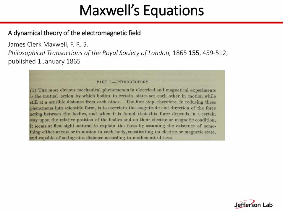
A dynamical theory of the electromagnetic field

James Clerk Maxwell, F. R. S.Philosophical Transactions of the Royal Society of London, 1865 155, 459-512, published 1 January 1865

Maxwell’s Equations

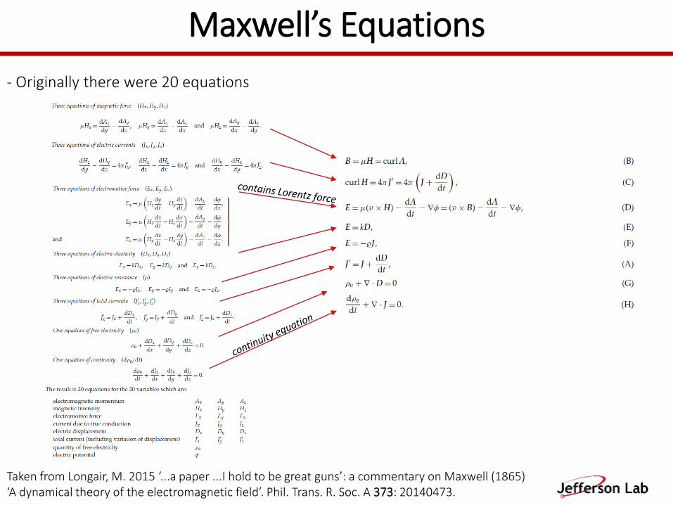
Taken from Longair, M. 2015 ‘...a paper ...I hold to be great guns’: a commentary on Maxwell (1865) ‘A dynamical theory of the electromagnetic field’. Phil. Trans. R. Soc. A 373: 20140473.

- Originally there were 20 equations

Sources of Electromagnetic Fields

5

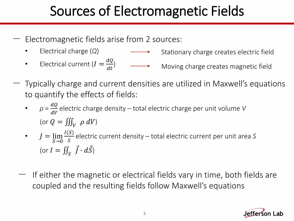
－ Electromagnetic fields arise from 2 sources:

• Electrical charge (Q)

• Electrical current (𝐼 =𝑑𝑄

𝑑𝑡)

－ Typically charge and current densities are utilized in Maxwell’s equations to quantify the effects of fields:

• ρ = 𝑑𝑄

𝑑𝑉electric charge density – total electric charge per unit volume V

(or 𝑄 = 𝑉 𝜌 𝑑𝑉)

• 𝐽 = lim𝑆→0

𝐼(𝑆)

𝑆electric current density – total electric current per unit area S

(or 𝐼 = 𝑆 𝐽 ∙ 𝑑 𝑆)

Stationary charge creates electric field

Moving charge creates magnetic field

－ If either the magnetic or electrical fields vary in time, both fields are coupled and the resulting fields follow Maxwell’s equations

Maxwell’s Equations

6

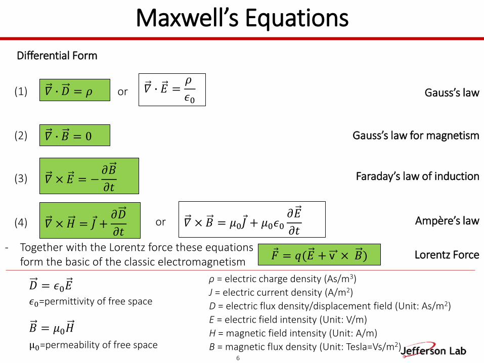
𝛻 ∙ 𝐷 = 𝜌

𝛻 × 𝐸 = −𝜕𝐵

𝜕𝑡

𝛻 ∙ 𝐵 = 0

𝛻 × 𝐻 = 𝐽 +𝜕𝐷

𝜕𝑡

𝐷 = 𝜖0𝐸

𝐵 = 𝜇0𝐻

Differential Form

D = electric flux density/displacement field (Unit: As/m2)

E = electric field intensity (Unit: V/m)

ρ = electric charge density (As/m3)

H = magnetic field intensity (Unit: A/m)

B = magnetic flux density (Unit: Tesla=Vs/m2)

J = electric current density (A/m2)

𝛻 ∙ 𝐸 =𝜌

𝜖0

𝜖0=permittivity of free space

𝛻 × 𝐵 = 𝜇0 𝐽 + 𝜇0𝜖0𝜕𝐸

𝜕𝑡

µ0=permeability of free space

or

or

Gauss’s law

Gauss’s law for magnetism

Ampère’s law

Faraday’s law of induction

(1)

(2)

(3)

(4)

𝐹 = 𝑞(𝐸 + v × 𝐵)- Together with the Lorentz force these equations

form the basic of the classic electromagnetismLorentz Force

Divergence (Gauss’) Theorem

7

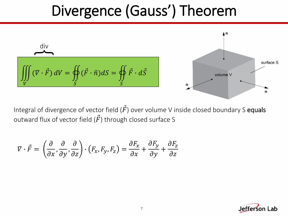
Integral of divergence of vector field ( 𝐹) over volume V inside closed boundary S equals

outward flux of vector field ( 𝐹) through closed surface S

𝑉

(𝛻 ∙ 𝐹) 𝑑𝑉 =

𝑆

( 𝐹 ∙ 𝑛)𝑑𝑆 =

𝑆

𝐹 ∙ 𝑑 𝑆

div

𝛻 ∙ 𝐹 =𝜕

𝜕𝑥,𝜕

𝜕𝑦,𝜕

𝜕𝑧∙ 𝐹𝑥, 𝐹𝑦 , 𝐹𝑧 =

𝜕𝐹𝑥𝜕𝑥+𝜕𝐹𝑦

𝜕𝑦+𝜕𝐹𝑧𝜕𝑧

𝑆

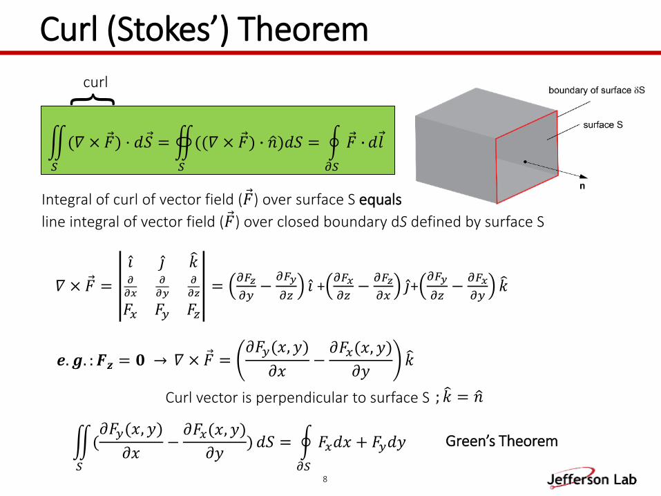
(𝜕𝐹𝑦(𝑥, 𝑦)

𝜕𝑥−𝜕𝐹𝑥(𝑥, 𝑦)

𝜕𝑦) 𝑑𝑆 =

𝜕𝑆

𝐹𝑥𝑑𝑥 + 𝐹𝑦𝑑𝑦

Curl (Stokes’) Theorem

8

𝑆

(𝛻 × 𝐹) · 𝑑 𝑆 =

𝑆

((𝛻 × 𝐹) ∙ 𝑛)𝑑𝑆 =

𝜕𝑆

𝐹 ∙ 𝑑 𝑙

Green’s Theorem

curl

𝒆. 𝒈. : 𝑭𝒛 = 𝟎 → 𝛻 × 𝐹 =𝜕𝐹𝑦(𝑥, 𝑦)

𝜕𝑥−𝜕𝐹𝑥(𝑥, 𝑦)

𝜕𝑦 𝑘

Integral of curl of vector field ( 𝐹) over surface S equals

line integral of vector field ( 𝐹) over closed boundary dS defined by surface S

; 𝑘 = 𝑛Curl vector is perpendicular to surface S

𝛻 × 𝐹 =

𝑖 𝑗 𝑘𝜕

𝜕𝑥

𝜕

𝜕𝑦

𝜕

𝜕𝑧

𝐹𝑥 𝐹𝑦 𝐹𝑧

=𝜕𝐹𝑧

𝜕𝑦−𝜕𝐹𝑦

𝜕𝑧 𝑖 +𝜕𝐹𝑥

𝜕𝑧−𝜕𝐹𝑧

𝜕𝑥 𝑗+𝜕𝐹𝑦

𝜕𝑧−𝜕𝐹𝑥

𝜕𝑦 𝑘

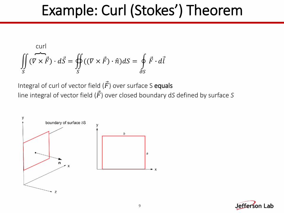
Example: Curl (Stokes’) Theorem

9

Integral of curl of vector field ( 𝐹) over surface S equals

line integral of vector field ( 𝐹) over closed boundary dS defined by surface S

𝑆

(𝛻 × 𝐹) · 𝑑 𝑆 =

𝑆

((𝛻 × 𝐹) ∙ 𝑛)𝑑𝑆 =

𝜕𝑆

𝐹 ∙ 𝑑 𝑙

curl

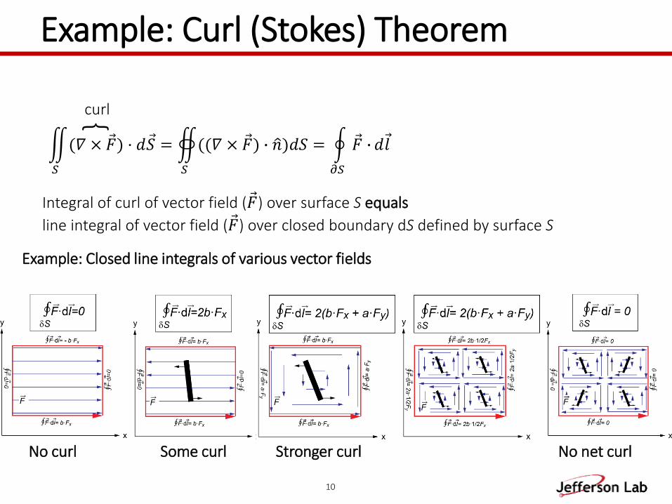
Example: Curl (Stokes) Theorem

10

𝑆

(𝛻 × 𝐹) · 𝑑 𝑆 =

𝑆

((𝛻 × 𝐹) ∙ 𝑛)𝑑𝑆 =

𝜕𝑆

𝐹 ∙ 𝑑 𝑙

Example: Closed line integrals of various vector fields

curl

Integral of curl of vector field ( 𝐹) over surface S equals

line integral of vector field ( 𝐹) over closed boundary dS defined by surface S

No curl Some curl Stronger curl No net curl

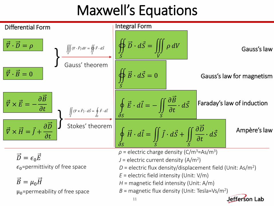
Maxwell’s Equations

11

𝛻 ∙ 𝐷 = 𝜌

𝛻 × 𝐸 = −𝜕𝐵

𝜕𝑡

𝛻 ∙ 𝐵 = 0

𝛻 × 𝐻 = 𝐽 +𝜕𝐷

𝜕𝑡

Differential Form Integral Form

D = electric flux density/displacement field (Unit: As/m2)

E = electric field intensity (Unit: V/m)

H = magnetic field intensity (Unit: A/m)

B = magnetic flux density (Unit: Tesla=Vs/m2)

J = electric current density (A/m2)

Gauss’ theorem

Stokes’ theorem

𝐷 = 𝜖0𝐸

𝐵 = 𝜇0𝐻

𝜖0=permittivity of free space

µ0=permeability of free space

𝑆

𝐷 ∙ 𝑑 𝑆 =

𝑉

𝜌 𝑑𝑉

𝑆

𝐵 ∙ 𝑑 𝑆 = 0

𝜕𝑆

𝐸 ∙ 𝑑 𝑙 = −

𝑆

𝜕𝐵

𝜕𝑡∙ 𝑑 𝑆

𝜕𝑆

𝐻 ∙ 𝑑 𝑙 =

𝑆

𝐽 ∙ 𝑑 𝑆 +

𝑆

𝜕𝐷

𝜕𝑡∙ 𝑑 𝑆

Gauss’s law

Gauss’s law for magnetism

Ampère’s law

Faraday’s law of induction

𝑉

(𝛻 ∙ 𝐹) 𝑑𝑉 =

𝑆

𝐹 ∙ 𝑑 𝑆

𝑆

(𝛻 × 𝐹) · 𝑑 𝑆 =

𝜕𝑆

𝐹 ∙ 𝑑 𝑙

ρ = electric charge density (C/m3=As/m3)

12

; 𝐷 = 𝜖0𝐸

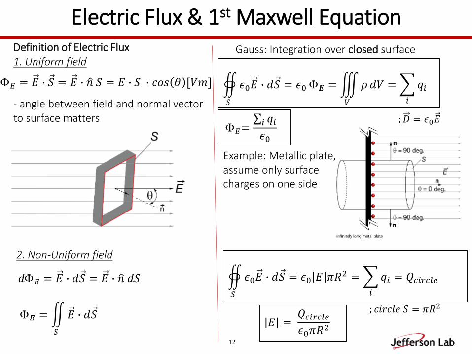
1. Uniform field

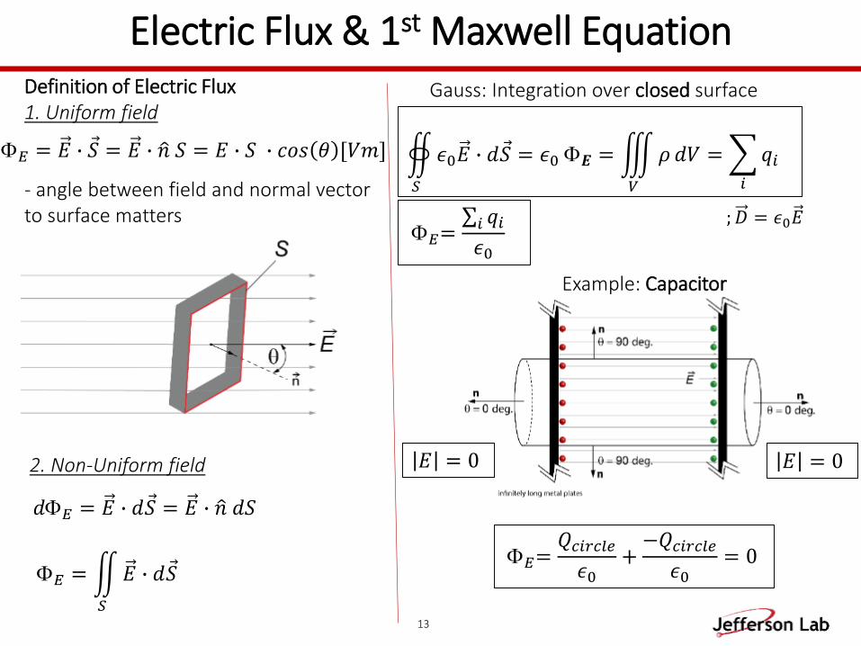
Electric Flux & 1st Maxwell Equation

𝐸 = 𝐸 ∙ 𝑆 = 𝐸 ∙ 𝑛 𝑆 = 𝐸 ∙ 𝑆 ∙ 𝑐𝑜𝑠 𝜃 [𝑉𝑚]

; 𝑐𝑖𝑟𝑐𝑙𝑒 𝑆 = 𝜋𝑅2

𝑆

𝜖0𝐸 ∙ 𝑑 𝑆 = 𝜖0 𝐸 𝜋𝑅2 =

𝑖

𝑞𝑖 = 𝑄𝑐𝑖𝑟𝑐𝑙𝑒

𝐸 =𝑄𝑐𝑖𝑟𝑐𝑙𝑒𝜖0𝜋𝑅

2

- angle between field and normal vectorto surface matters

𝑆

𝜖0𝐸 ∙ 𝑑 𝑆 = 𝜖0 𝑬 =

𝑉

𝜌 𝑑𝑉 =

𝑖

𝑞𝑖

Gauss: Integration over closed surface

𝐸= 𝑖 𝑞𝑖𝜖0

2. Non-Uniform field

𝑑𝐸 = 𝐸 ∙ 𝑑 𝑆 = 𝐸 ∙ 𝑛 𝑑𝑆

𝐸 =

𝑆

𝐸 ∙ 𝑑 𝑆

Example: Metallic plate,assume only surface charges on one side

Definition of Electric Flux

13

Gauss: Integration over closed surface

𝐸 = 0

𝐸=𝑄𝑐𝑖𝑟𝑐𝑙𝑒𝜖0

+−𝑄𝑐𝑖𝑟𝑐𝑙𝑒𝜖0

= 0

𝐸 = 0

Example: Capacitor

Electric Flux & 1st Maxwell Equation

1. Uniform field

𝐸 = 𝐸 ∙ 𝑆 = 𝐸 ∙ 𝑛 𝑆 = 𝐸 ∙ 𝑆 ∙ 𝑐𝑜𝑠 𝜃 [𝑉𝑚]

- angle between field and normal vectorto surface matters

2. Non-Uniform field

𝑑𝐸 = 𝐸 ∙ 𝑑 𝑆 = 𝐸 ∙ 𝑛 𝑑𝑆

𝐸 =

𝑆

𝐸 ∙ 𝑑 𝑆

Definition of Electric Flux

; 𝐷 = 𝜖0𝐸

𝑆

𝜖0𝐸 ∙ 𝑑 𝑆 = 𝜖0 𝑬 =

𝑉

𝜌 𝑑𝑉 =

𝑖

𝑞𝑖

𝐸= 𝑖 𝑞𝑖𝜖0

14

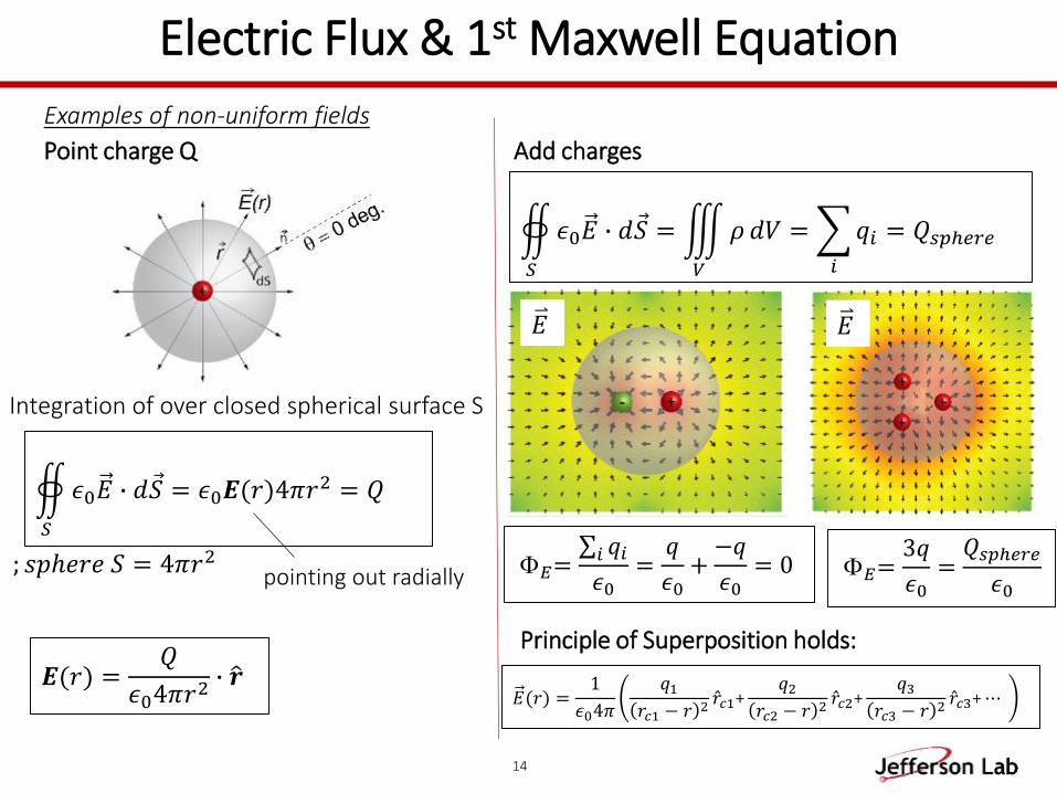
Integration of over closed spherical surface S

𝑬(𝑟) =𝑄

𝜖04𝜋𝑟2∙ 𝒓

; 𝑠𝑝ℎ𝑒𝑟𝑒 𝑆 = 4𝜋𝑟2

Examples of non-uniform fields

Point charge Q

𝑆

𝜖0𝐸 ∙ 𝑑 𝑆 = 𝜖0𝑬(𝑟)4𝜋𝑟2 = 𝑄

𝑆

𝜖0𝐸 ∙ 𝑑 𝑆 =

𝑉

𝜌 𝑑𝑉 =

𝑖

𝑞𝑖 = 𝑄𝑠𝑝ℎ𝑒𝑟𝑒

𝐸= 𝑖 𝑞𝑖𝜖0=𝑞

𝜖0+−𝑞

𝜖0= 0 𝐸=

3𝑞

𝜖0=𝑄𝑠𝑝ℎ𝑒𝑟𝑒

𝜖0

Principle of Superposition holds:

𝐸(𝑟) =1

𝜖04𝜋

𝑞1𝑟𝑐1 − 𝑟 2

𝑟𝑐1+𝑞2

𝑟𝑐2 − 𝑟 2 𝑟𝑐2+

𝑞3𝑟𝑐3 − 𝑟 2

𝑟𝑐3+⋯

Electric Flux & 1st Maxwell Equation

𝐸 𝐸

pointing out radially

Add charges

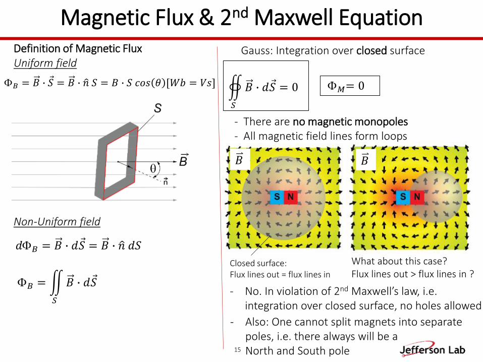
𝐵 = 𝐵 ∙ 𝑆 = 𝐵 ∙ 𝑛 𝑆 = 𝐵 ∙ 𝑆 𝑐𝑜𝑠 𝜃 [𝑊𝑏 = 𝑉𝑠]

15

Uniform field

Magnetic Flux & 2nd Maxwell EquationGauss: Integration over closed surface

𝑀= 0

Non-Uniform field

𝑑𝐵 = 𝐵 ∙ 𝑑 𝑆 = 𝐵 ∙ 𝑛 𝑑𝑆

𝐵 =

𝑆

𝐵 ∙ 𝑑 𝑆

Definition of Magnetic Flux

𝑆

𝐵 ∙ 𝑑 𝑆 = 0

- There are no magnetic monopoles- All magnetic field lines form loops

𝐵

Closed surface:Flux lines out = flux lines in

What about this case?Flux lines out > flux lines in ?

- No. In violation of 2nd Maxwell’s law, i.e. integration over closed surface, no holes allowed

𝐵

- Also: One cannot split magnets into separate poles, i.e. there always will be a North and South pole

16

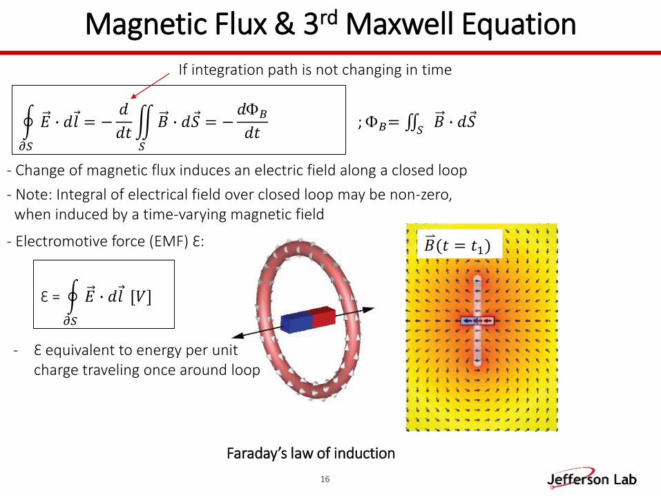
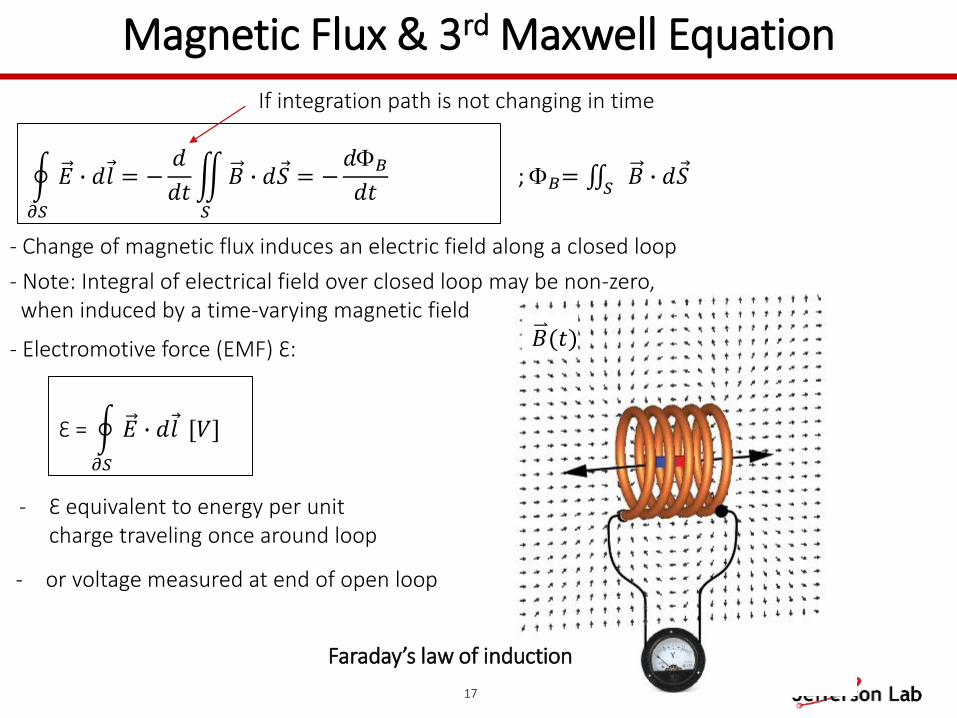
𝜕𝑆

𝐸 ∙ 𝑑 𝑙 = −𝑑

𝑑𝑡

𝑆

𝐵 ∙ 𝑑 𝑆 = −𝑑𝐵𝑑𝑡

Magnetic Flux & 3rd Maxwell Equation

𝐵(𝑡 = 𝑡1)

Faraday’s law of induction

If integration path is not changing in time

; 𝐵= 𝑆 𝐵 ∙ 𝑑 𝑆

- Change of magnetic flux induces an electric field along a closed loop

- Note: Integral of electrical field over closed loop may be non-zero, when induced by a time-varying magnetic field

Ɛ =

𝜕𝑆

𝐸 ∙ 𝑑 𝑙 [𝑉]

- Electromotive force (EMF) Ɛ:

- Ɛ equivalent to energy per unitcharge traveling once around loop

17

; 𝐵= 𝑆 𝐵 ∙ 𝑑 𝑆

- Change of magnetic flux induces an electric field along a closed loop

𝜕𝑆

𝐸 ∙ 𝑑 𝑙 = −𝑑

𝑑𝑡

𝑆

𝐵 ∙ 𝑑 𝑆 = −𝑑𝐵𝑑𝑡

Magnetic Flux & 3rd Maxwell Equation

Ɛ =

𝜕𝑆

𝐸 ∙ 𝑑 𝑙 [𝑉]

- Electromotive force (EMF) Ɛ:

- Note: Integral of electrical field over closed loop may be non-zero, when induced by a time-varying magnetic field

𝐵(𝑡)

If integration path is not changing in time

- Ɛ equivalent to energy per unitcharge traveling once around loop

- or voltage measured at end of open loop

Faraday’s law of induction

18

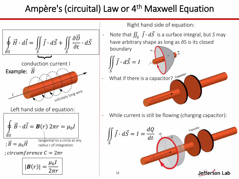
Ampère's (circuital) Law or 4th Maxwell Equation

- Note that 𝑆 𝐽 ∙ 𝑑 𝑆 is a surface integral, but S may

have arbitrary shape as long as ∂S is its closed boundary

- What if there is a capacitor?

𝑆

𝐽 ∙ 𝑑 𝑆 = 𝐼

- While current is still be flowing (charging capacitor):

𝑆

𝐽 ∙ 𝑑 𝑆 = 𝐼 =𝑑𝑄

𝑑𝑡

𝜕𝑆

𝐻 ∙ 𝑑 𝑙 =

𝑆

𝐽 ∙ 𝑑 𝑆 +

𝑆

𝜕𝐷

𝜕𝑡∙ 𝑑 𝑆

; 𝐵 = 𝜇0𝐻

; 𝑐𝑖𝑟𝑐𝑢𝑚𝑓𝑒𝑟𝑒𝑛𝑐𝑒 𝐶 = 2𝜋𝑟

𝜕𝑆

𝐵 ∙ 𝑑 𝑙 = 𝑩 𝑟 2𝜋𝑟 = 𝜇0𝐼

𝐵Example:

tangential to a circle at any radius r of integration

conduction current I

|𝑩 𝑟 | =𝜇0𝐼

2𝜋𝑟

Right hand side of equation:

Left hand side of equation:

19

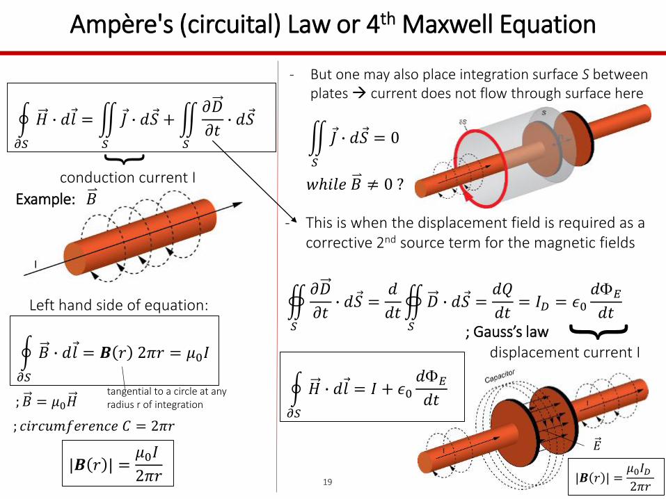
Ampère's (circuital) Law or 4th Maxwell Equation

𝜕𝑆

𝐻 ∙ 𝑑 𝑙 =

𝑆

𝐽 ∙ 𝑑 𝑆 +

𝑆

𝜕𝐷

𝜕𝑡∙ 𝑑 𝑆

; 𝐵 = 𝜇0𝐻

; 𝑐𝑖𝑟𝑐𝑢𝑚𝑓𝑒𝑟𝑒𝑛𝑐𝑒 𝐶 = 2𝜋𝑟

𝜕𝑆

𝐵 ∙ 𝑑 𝑙 = 𝑩 𝑟 2𝜋𝑟 = 𝜇0𝐼

|𝑩 𝑟 | =𝜇0𝐼

2𝜋𝑟

displacement current I

𝑆

𝜕𝐷

𝜕𝑡∙ 𝑑 𝑆 =

𝑑

𝑑𝑡

𝑆

𝐷 ∙ 𝑑 𝑆 =𝑑𝑄

𝑑𝑡= 𝐼𝐷 = 𝜖0

𝑑𝐸𝑑𝑡

- But one may also place integration surface S between plates current does not flow through surface here

𝑆

𝐽 ∙ 𝑑 𝑆 = 0

𝑤ℎ𝑖𝑙𝑒 𝐵 ≠ 0 ?

- This is when the displacement field is required as a corrective 2nd source term for the magnetic fields

tangential to a circle at any radius r of integration

; Gauss’s law

𝐵

𝐸

|𝑩 𝑟 | =𝜇0𝐼𝐷2𝜋𝑟

conduction current I

𝐵Example:

Left hand side of equation:

𝜕𝑆

𝐻 ∙ 𝑑 𝑙 = 𝐼 + 𝜖0𝑑𝐸𝑑𝑡

20

𝜕𝑆

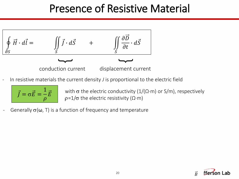
𝐻 ∙ 𝑑 𝑙 =

𝑆

𝐽 ∙ 𝑑 𝑆 +

𝑆

𝜕𝐷

𝜕𝑡∙ 𝑑 𝑆

conduction current

𝐵

displacement current

- In resistive materials the current density J is proportional to the electric field

𝐽 = 𝐸 =1

𝜌𝐸

with the electric conductivity (1/(Ω·m) or S/m), respectively=1/ the electric resistivity (Ω·m)

- Generally (ω, T) is a function of frequency and temperature

Presence of Resistive Material

21

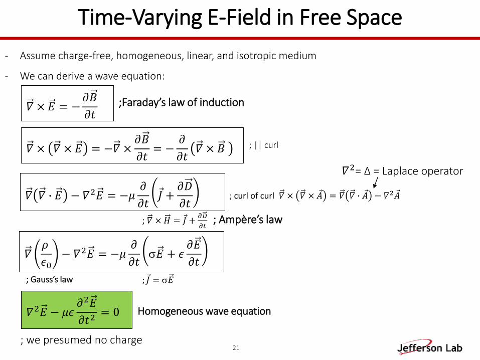
- We can derive a wave equation:

Time-Varying E-Field in Free Space

𝛻 × 𝐸 = −𝜕𝐵

𝜕𝑡;Faraday’s law of induction

𝛻 × 𝛻 × 𝐸 = −𝛻 ×𝜕𝐵

𝜕𝑡= −

𝜕

𝜕𝑡𝛻 × 𝐵

; curl of curl 𝛻 × 𝛻 × 𝐴 = 𝛻 𝛻 ∙ 𝐴 − 𝛻2 𝐴

; || curl

𝛻 𝛻 ∙ 𝐸 − 𝛻2𝐸 = −𝜇𝜕

𝜕𝑡 𝐽 +𝜕𝐷

𝜕𝑡

; Ampère’s law

𝛻𝜌

𝜖0− 𝛻2𝐸 = −𝜇

𝜕

𝜕𝑡𝐸 + 𝜖

𝜕𝐸

𝜕𝑡

; Gauss’s law ; 𝐽 = 𝐸

𝛻2= Δ = Laplace operator

𝛻2𝐸 − 𝜇𝜖𝜕2𝐸

𝜕𝑡2= 0

; we presumed no charge

- Assume charge-free, homogeneous, linear, and isotropic medium

; 𝛻 × 𝐻 = 𝐽 +𝜕𝐷

𝜕𝑡

Homogeneous wave equation

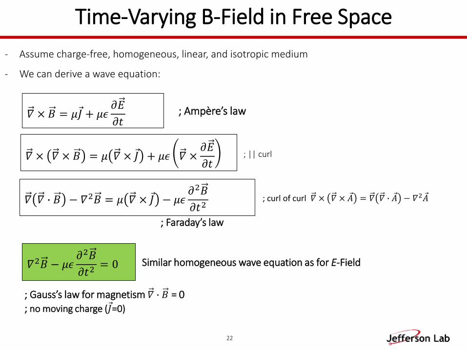
22

Time-Varying B-Field in Free Space

; Ampère’s law

𝛻 × 𝛻 × 𝐵 = 𝜇 𝛻 × 𝐽 + 𝜇𝜖 𝛻 ×𝜕𝐸

𝜕𝑡

𝛻 𝛻 ∙ 𝐵 − 𝛻2𝐵 = 𝜇 𝛻 × 𝐽 − 𝜇𝜖𝜕2𝐵

𝜕𝑡2

; Faraday’s law

𝛻 × 𝐵 = 𝜇 𝐽 + 𝜇𝜖𝜕𝐸

𝜕𝑡

; Gauss’s law for magnetism 𝛻 ∙ 𝐵 = 0

; no moving charge ( 𝐽=0)

𝛻2𝐵 − 𝜇𝜖𝜕2𝐵

𝜕𝑡2= 0 Similar homogeneous wave equation as for E-Field

- We can derive a wave equation:

- Assume charge-free, homogeneous, linear, and isotropic medium

; || curl

; curl of curl 𝛻 × 𝛻 × 𝐴 = 𝛻 𝛻 ∙ 𝐴 − 𝛻2 𝐴

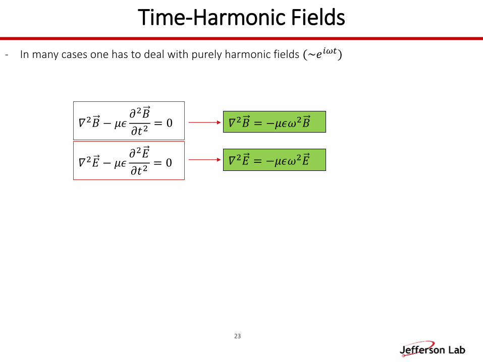
23

- In many cases one has to deal with purely harmonic fields (~𝑒𝑖𝜔𝑡)

Time-Harmonic Fields

𝛻2𝐸 − 𝜇𝜖𝜕2𝐸

𝜕𝑡2= 0

𝛻2𝐵 = −𝜇𝜖𝜔2𝐵

𝛻2𝐸 = −𝜇𝜖𝜔2𝐸

𝛻2𝐵 − 𝜇𝜖𝜕2𝐵

𝜕𝑡2= 0

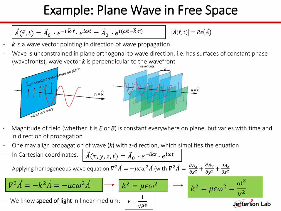
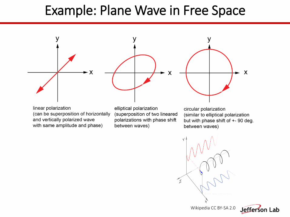
Example: Plane Wave in Free Space

𝐴( 𝑟, 𝑡) = 𝐴0 ∙ 𝑒−𝑖 𝑘∙ 𝑟∙ 𝑒𝑖𝜔𝑡 = 𝐴0 ∙ 𝑒

𝑖(𝜔𝑡−𝑘∙ 𝑟)

- k is a wave vector pointing in direction of wave propagation

𝐴( 𝑟, 𝑡) = 𝑅𝑒 𝐴

- Wave is unconstrained in plane orthogonal to wave direction, i.e. has surfaces of constant phase (wavefronts), wave vector k is perpendicular to the wavefront

- In Cartesian coordinates: 𝐴(𝑥, 𝑦, 𝑧, 𝑡) = 𝐴0 ∙ 𝑒−𝑖𝑘𝑧 ∙ 𝑒𝑖𝜔𝑡

- One may align propagation of wave (k) with z-direction, which simplifies the equation

𝛻2 𝐴 = −𝑘2 𝐴 = −𝜇𝜖𝜔2 𝐴

- Magnitude of field (whether it is E or B) is constant everywhere on plane, but varies with time and in direction of propagation

𝑘2 = 𝜇𝜖𝜔2

𝘷 =1

𝜇𝜖

- Applying homogeneous wave equation 𝛻2 𝐴 = −𝜇𝜖𝜔2 𝐴 (with 𝛻2 𝐴 =𝜕𝐴𝑥

𝜕𝑥2+𝜕𝐴𝑦

𝜕𝑦2+𝜕𝐴𝑧

𝜕𝑧2

- We know speed of light in linear medium:

𝑘2 = 𝜇𝜖𝜔2 =𝜔2

𝘷2

Example: Plane Wave in Free Space

Wikipedia CC BY-SA 2.0

26

Example: Plane Wave in Free Space

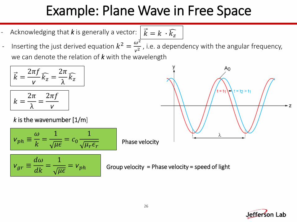
k is the wavenumber [1/m]

𝘷𝑔𝑟 ≡𝑑𝜔

𝑑𝑘=1

𝜇𝜖= 𝘷𝑝ℎ

𝘷𝑝ℎ ≡𝜔

𝑘=1

𝜇𝜖= 𝑐0

1

𝜇𝑟𝜖𝑟

𝑘 = 𝑘 ∙ 𝑘𝑧

Phase velocity

Group velocity

𝑘 =2𝜋

λ=2𝜋𝑓

𝘷

- Acknowledging that k is generally a vector:

𝑘 =2𝜋𝑓

𝘷 𝑘𝑧 =

2𝜋

λ 𝑘𝑧

- Inserting the just derived equation 𝑘2 =𝜔2

𝘷2, i.e. a dependency with the angular frequency,

we can denote the relation of k with the wavelength

= Phase velocity = speed of light

27

Wave Impedance

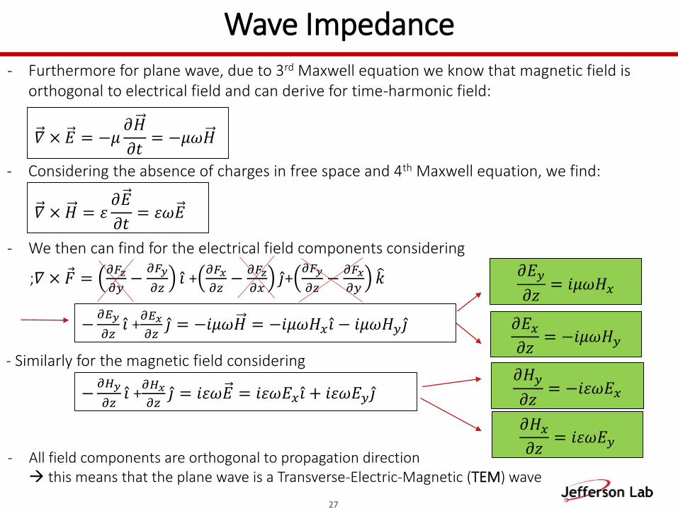
;𝛻 × 𝐹 =𝜕𝐹𝑧

𝜕𝑦−𝜕𝐹𝑦

𝜕𝑧 𝑖 +𝜕𝐹𝑥

𝜕𝑧−𝜕𝐹𝑧

𝜕𝑥 𝑗+𝜕𝐹𝑦

𝜕𝑧−𝜕𝐹𝑥

𝜕𝑦 𝑘

𝜕𝐻𝑥𝜕𝑧= 𝑖𝜀𝜔𝐸𝑦

𝜕𝐻𝑦

𝜕𝑧= −𝑖𝜀𝜔𝐸𝑥−

𝜕𝐻𝑦

𝜕𝑧 𝑖 +𝜕𝐻𝑥

𝜕𝑧 𝑗 = 𝑖𝜀𝜔𝐸 = 𝑖𝜀𝜔𝐸𝑥 𝑖 + 𝑖𝜀𝜔𝐸𝑦 𝑗

- Similarly for the magnetic field considering

- All field components are orthogonal to propagation direction this means that the plane wave is a Transverse-Electric-Magnetic (TEM) wave

𝛻 × 𝐸 = −𝜇𝜕𝐻

𝜕𝑡= −𝜇𝜔𝐻

𝛻 × 𝐻 = 𝜀𝜕𝐸

𝜕𝑡= 𝜀𝜔𝐸

- We then can find for the electrical field components considering

- Considering the absence of charges in free space and 4th Maxwell equation, we find:

- Furthermore for plane wave, due to 3rd Maxwell equation we know that magnetic field is orthogonal to electrical field and can derive for time-harmonic field:

−𝜕𝐸𝑦

𝜕𝑧 𝑖 +𝜕𝐸𝑥

𝜕𝑧 𝑗 = −𝑖𝜇𝜔𝐻 = −𝑖𝜇𝜔𝐻𝑥 𝑖 − 𝑖𝜇𝜔𝐻𝑦 𝑗 𝜕𝐸𝑥

𝜕𝑧= −𝑖𝜇𝜔𝐻𝑦

𝜕𝐸𝑦

𝜕𝑧= 𝑖𝜇𝜔𝐻𝑥

28

Wave Impedance

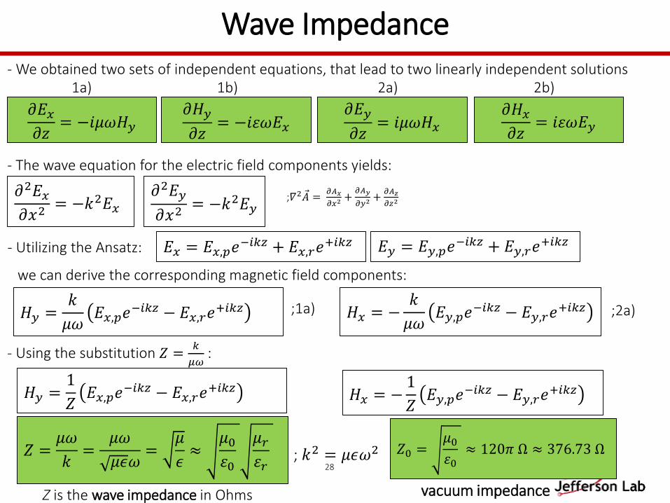
𝜕𝐸𝑥𝜕𝑧= −𝑖𝜇𝜔𝐻𝑦

𝜕𝐸𝑦

𝜕𝑧= 𝑖𝜇𝜔𝐻𝑥

𝜕𝐻𝑥𝜕𝑧= 𝑖𝜀𝜔𝐸𝑦

𝜕𝐻𝑦

𝜕𝑧= −𝑖𝜀𝜔𝐸𝑥

- We obtained two sets of independent equations, that lead to two linearly independent solutions

;𝛻2 𝐴 =𝜕𝐴𝑥

𝜕𝑥2+𝜕𝐴𝑦

𝜕𝑦2+𝜕𝐴𝑧

𝜕𝑧2𝜕2𝐸𝑥𝜕𝑥2

= −𝑘2𝐸𝑥𝜕2𝐸𝑦

𝜕𝑥2= −𝑘2𝐸𝑦

- The wave equation for the electric field components yields:

- Utilizing the Ansatz: 𝐸𝑥 = 𝐸𝑥,𝑝𝑒−𝑖𝑘𝑧 + 𝐸𝑥,𝑟𝑒

+𝑖𝑘𝑧 𝐸𝑦 = 𝐸𝑦,𝑝𝑒−𝑖𝑘𝑧 + 𝐸𝑦,𝑟𝑒

+𝑖𝑘𝑧

𝐻𝑥 = −𝑘

𝜇𝜔𝐸𝑦,𝑝𝑒

−𝑖𝑘𝑧 − 𝐸𝑦,𝑟𝑒+𝑖𝑘𝑧𝐻𝑦 =

𝑘

𝜇𝜔𝐸𝑥,𝑝𝑒

−𝑖𝑘𝑧 − 𝐸𝑥,𝑟𝑒+𝑖𝑘𝑧

1a) 2a) 2b)1b)

;2a);1a)

we can derive the corresponding magnetic field components:

𝑍 =𝜇𝜔

𝑘=𝜇𝜔

𝜇𝜖𝜔=𝜇

𝜖≈𝜇0𝜀0

𝜇𝑟𝜀𝑟

; 𝑘2 = 𝜇𝜖𝜔2

- Using the substitution 𝑍 =𝑘

𝜇𝜔:

𝑍0 =𝜇0𝜀0≈ 120𝜋 Ω ≈ 376.73 Ω

vacuum impedanceZ is the wave impedance in Ohms

𝐻𝑦 =1

𝑍𝐸𝑥,𝑝𝑒

−𝑖𝑘𝑧 − 𝐸𝑥,𝑟𝑒+𝑖𝑘𝑧 𝐻𝑥 = −

1

𝑍𝐸𝑦,𝑝𝑒

−𝑖𝑘𝑧 − 𝐸𝑦,𝑟𝑒+𝑖𝑘𝑧

Appendix

Presence of Dielectric Material

30

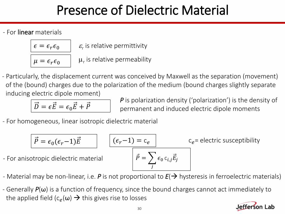
- For linear materials

𝜖 = 𝜖𝑟𝜖0

𝜇 = 𝜖𝑟𝜖0

r is relative permittivity

r is relative permeability

- Particularly, the displacement current was conceived by Maxwell as the separation (movement) of the (bound) charges due to the polarization of the medium (bound charges slightly separate inducing electric dipole moment)

𝐷 = 𝜖𝐸 = 𝜖0𝐸 + 𝑃

- For homogeneous, linear isotropic dielectric material

𝑃 = 𝜖0(𝜖𝑟−1)𝐸 (𝜖𝑟−1) = c𝑒 c𝑒= electric susceptibility

- For anisotropic dielectric material 𝑃 =

𝑗

𝜖0 c𝑖,𝑗𝐸𝑗

- Material may be non-linear, i.e. P is not proportional to E( hysteresis in ferroelectric materials)

- Generally P(ω) is a function of frequency, since the bound charges cannot act immediately to the applied field (c𝑒(ω) this gives rise to losses

P is polarization density (‘polarization’) is the density of permanent and induced electric dipole moments

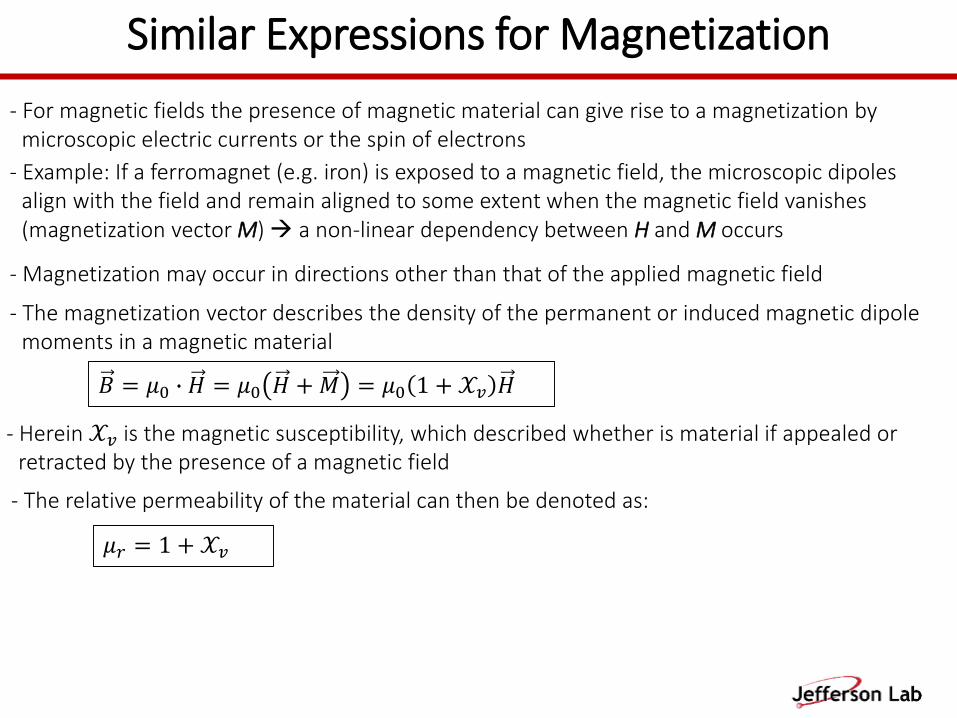
Similar Expressions for Magnetization

𝐵 = 𝜇0 ∙ 𝐻 = 𝜇0 𝐻 +𝑀 = 𝜇0 1 + 𝒳𝑣 𝐻

- For magnetic fields the presence of magnetic material can give rise to a magnetization by microscopic electric currents or the spin of electrons

- The magnetization vector describes the density of the permanent or induced magnetic dipole moments in a magnetic material

- Herein 𝒳𝑣 is the magnetic susceptibility, which described whether is material if appealed or retracted by the presence of a magnetic field

- The relative permeability of the material can then be denoted as:

𝜇𝑟 = 1 +𝒳𝑣

- Magnetization may occur in directions other than that of the applied magnetic field

- Example: If a ferromagnet (e.g. iron) is exposed to a magnetic field, the microscopic dipoles align with the field and remain aligned to some extent when the magnetic field vanishes (magnetization vector M) a non-linear dependency between H and M occurs