Embed Size (px)
Citation preview

Lecture II: Matrix Functions in Network Science, Part 1
Michele Benzi
Department of Mathematics and Computer ScienceEmory University
Atlanta, Georgia, USA
Summer School on Theory and Computation of Matrix Functions
Dobbiaco, 15-20 June, 2014
1

Outline
1 Complex networks: motivation and background
2 Network structure: centrality and communicability measures
3 Bibliography
2

Outline
1 Complex networks: motivation and background
2 Network structure: centrality and communicability measures
3 Bibliography
3

Complex networks: motivation and background
Networks, in particular complex networks, provide models for a widevariety of physical, biological, engineered or social systems.
For example: molecular structure, gene and protein interaction, anatomicaland metabolic networks, food webs, transportation networks, power grids,financial and trade networks, social networks, the Internet, the WWW,Facebook, Twitter ...
Network Science is the study of networks, both as mathematical structuresand as concrete, real world objects. It is a growing multidisciplinary field,with important contributions not just from mathematicians, computerscientists and physicists but also from social scientists, biologists, publichealth researchers and even from scholars in the humanities.
4

Complex networks: motivation and background (cont.)
The field has its origins in the work of psychologists, sociologists,economists, anthropologists and statisticians dating back to the late 1940sand early 1950s. In the last 15 years or so, physicists, computer scientistsand mathematicians have entered the scene and made the field moremathematically sophisticated.
Basic tools for the analysis of networks include graph theory, linearalgebra, probability, numerical analysis, and of course algorithms and datastructures from discrete mathematics. More advanced techniques includestatistical mechanics and multilinear algebra.
The study of dynamical processes often leads to differential equationsposed on networks.
5

Basic references
Some classic early references:
J. R. Seeley, The net of reciprocal influence: A problem in treatingsociometric data, Canadian J. Psychology, 3 (1949), pp. 234–240.
L. Katz, A new status index derived from sociometric analysis,Psychometrika, 18 (1953), pp. 39–43.
A. Rapoport, Mathematical models of social interaction, in Handbook ofMathematical Psychology, vol. 2, pp. 493–579. Wiley, New York, 1963.
D. J. de Solla Price, Networks of scientific papers, Science, 149 (1965),pp. 510–515.
S. Milgram, The small world problem, Psychology Today, 2 (1967),pp. 60–67.
J. Travers and S. Milgram, An experimental study of the small worldproblem, Sociometry, 32 (1969), pp. 425–443.
6

Two pioneers of network science
Anatol Rapoport (1911-2007) and Stanley Milgram (1933-1984)
7

Basic references (cont.)
The field exploded in the late 1990s due to several breakthroughs byphysicists, applied mathematicians and computer scientists.
Landmark papers include
D. J. Watts and S. H. Strogatz, Collective dynamics of ‘small-world’networks, Nature, 393 (1998), pp. 440–442.
L.-A. Barabási and R. Albert, Emergence of scaling in random networks,Science, 386 (1999), pp. 509–512.
M. E. J. Newman, Models of the small world, J. Stat. Phys., 101 (2000),pp. 819–841.
J. Kleinberg, Navigation in a small world, Nature, 406 (2000), p. 845.
R. Albert and L.-A. Barabási, Statistical mechanics of complex networks,Rev. Modern Phys., 74 (2002), pp. 47–97.
8

Examples of complex networks
But what exactly is a complex network?
Unfortunately, no precise definition exists, although there is some ongoingwork on characterizing (and quantifying) the degree of complexity in anetwork.
It is easy to tell which graphs are not complex networks. Regular latticesare not considered complex networks, and neither are completely randomgraphs such as the Erdös–Rényi model.
Random graphs, however, are useful as null models against which tocompare (possible examples of) complex networks.
9

Regular lattice: not a complex network!
10

Star graph: not a complex network!
11

Erdös–Rényi graph: also not a complex network!
12

Some features of complex networks
Some of the attributes typical of many real-world complex networks are:
“Scale-free": the degree distribution follows a power law (Pareto’scurve)“Small-world":
I Small graph diameter, short average distance between nodesI High clustering coefficient: many triangles, hubs, ...
Hierarchical structureRich in “motifs"Self-similar (as in fractals)
Briefly stated: complex networks exhibit a non-trivial topology.
Caveat: there are important examples of real-world complex networks lacking oneor more of these attributes.
13

What a small world...!
Duncan Watts and Steven Strogatz
14

The Watts–Strogatz random rewire model
15

The rich always get richer!
Albert-László Barabási and Réka Albert
16

The Barabási–Albert model
The Barabási–Albert model is based on the notion of preferentialattachment: starting from a given sparse graph, new nodes are added (oneat a time) to the network, joining them to existing nodes with aprobability proportional to the degree (the number of adjacent nodes) ofsuch nodes. Hence, nodes that are rich of connections to other nodes havea high probability of attracting new “neighbors", while “poor" nodes tendto remain such.
One can show that the Barabási–Albert model leads to a highly skeweddegree distribution given by a power law of the form
p(k) ∝ k−γ ,
where p(k) denotes the fraction of nodes of degree k and γ is a constant,typically with 2 ≤ γ < 3.
17

The Barabási–Albert model (cont.)
Degree distribution according to a power law18

The Barabási–Albert model (cont.)
19

The Barabási–Albert model (cont.)
The Barabási–Albert model produces “small world" networks, in which thediameter grows slowly with the number of nodes; the growth is generallylogarithmic or even log-logarithmic (in practice, the diameter remainsnearly constant).
Examples: Facebook; MathSciNet collaboration graph.
Unlike the Barabási–Albert model, the Erdös–Rényi and Watts–Strogatzmodels exhibit degree distributions that decay exponentially from themean 〈k〉: hence, such networks are not “scale-free".
An overwhelming number of real-world complex networks appear to followa power law degree distribution, at least approximately.
20

Example of complex network: Golub collaboration graph
21

Example of complex network: Erdös collaboration graph
22

Example of complex network: PPI network ofSaccharomyces cerevisiae (beer yeast)
23

Example of complex network: social network of injectingdrug users in Colorado Springs, CO
Figure courtesy of Ernesto Estrada.
24

Example of complex network: a chunk of the Internet
25

Example of (directed) complex network: a food web
Picture credits: http://www.physicalgeography.net/fundamentals/9o.html
26

Network analysis
Basic questions about network structure include centrality, robustness,communicability and community detection issues:
Which are the most “important” nodes?I Network connectivity and robustness/vulnerabilityI Identification of influential individuals in social networksI Essential proteins in PPI networks (lethality)I Identification of keystone species in ecosystemsI Author centrality in collaboration networksI Ranking of documents/web pages on a given topic
How do “disturbances” spread in a network?I Spreading of epidemics, beliefs, rumors, fads,...I Routing of messages; bottlenecks, returnability
How to identify “community structures” in a network?I Clustering, triadic closure (transitivity)I Partitioning
27

Formal definitions
Real-world networks are usually modelled by means of graphs.
A graph G = (V,E) consists of a (finite) set V = {v1, v2, . . . , vN} ofnodes (or vertices) and a set E of edges (or links), which are pairs {vi, vj}with vi, vj ∈ V .
The graph G is directed if the edges {vi, vj} ∈ E are ordered pairs= (vi, vj) ∈ V × V , otherwise G is undirected. A directed graph is oftenreferred to as a digraph.
A loop in G is an edge from a node to itself. Loops are often ignored orexcluded.
A graph G is weighted if numerical values are associated with its edges.If all the edges are given the same value 1, we say that the graph isunweighted.
A simple graph is an unweighted graph without multiple edges or loops.
28

Formal definitions (cont.)
A walk of length k in G is a set of nodes vi1 , vi2 , . . . vik , vik+1such that for
all 1 ≤ j ≤ k, there is an edge between vij and vij+1 .
A closed walk is a walk where vi1 = vik+1.
A path is a walk with no repeated nodes.
A cycle is a path with an edge between the first and last node. In otherwords, a cycle is a closed path.
A triangle in G is a cycle of length 3.
29

Formal definitions (cont.)
The geodetic distance d(vi, vj) between two nodes is the length of theshortest path connecting vi and vj . We let d(vi, vj) = ∞ if no such pathexists.
The diameter of a graph G = (V,E) is defined as
diam(G) := maxvi,vj∈V
d(vi, vj) .
A graph G is connected if for every pair of nodes vi and vj there is a pathin G that starts at vi and ends at vj ; i.e., diam(G) < ∞.
These definitions apply to both undirected and directed graphs, though inthe latter case the orientation of the edges must be taken into account.
30

Formal definitions (cont.)
To every unweighted graph G = (V,E) we associate its adjacency matrixA = [aij ] ∈ RN×N , with
aij =
{1, if (vi, vj) ∈ E,0, else.
Any renumbering of the graph nodes results in a symmetric permutationA −→ PAP T of the adjacency matrix of the graph.
If G is an undirected graph, A is symmetric with zeros along the maindiagonal (A is “hollow”). In this case, the eigenvalues of A are all real.We label the eigenvalues of A in non-increasing order:λ1 ≥ λ2 ≥ · · · ≥ λN . Note that A is always indefinite if E 6= ∅.
If G is connected, then λ1 is simple and satisfies λ1 > λi for 2 ≤ i ≤ N(this follows from the Perron–Frobenius Theorem).
In particular, the spectral radius ρ(A) is given by λ1.31

Formal definitions (cont.)
If G is undirected, the degree di of node vi is the number of edges incidentto vi in G. In other words, di is the number of “immediate neighbors” of vi
in G. A regular graph is a graph where every node has the same degree d.
Note that in terms of the adjacency matrix, di =∑N
j=1 aij .
For a directed graph, we define the in-degree of node vi as the number dini
of edges ending in vi, and the out-degree of vi as the number douti of
edges originating at vi.
In terms of the (nonsymmetric) adjacency matrix,
dini =
N∑i=1
aij , douti =
N∑j=1
aij .
Hence, the column sums of A give the in-degrees and the row sums givethe out-degrees.
32

Formal definitions (cont.)
An undirected graph G = (V,E) is bipartite if there are V1, V2 ⊂ V , withV1, V2 6= ∅, V = V1 ∪ V2, V1 ∩ V2 = ∅ such that edges can exist onlybetween nodes belonging to different subsets V1, V2. In other terms, agraph is bipartite if it does not contain any odd-length cycles.
33

Formal definitions (cont.)
Let G = (V,E) be bipartite with |V1| = m, |V2| = n, m + n = N .
Then there exists a numbering of the nodes of G such that the adjacencymatrix of G is of the form
A =
[0 B
BT 0
]with B ∈ Rm×n.
Note: The nonzero eigenvalues of A are of the form ±σi, where σi denotethe singular values of B.
Bipartite graphs can also be used to give an alternative representation ofdirected graphs.
34

Formal definitions (cont.)
Indeed, given a digraph G = (V,E) with N nodes we can make a copyV ′ = {v′1, . . . , v′N} of V = {v1, . . . , vN} and define a new, undirectedgraph G = (V, E) wth 2N nodes, where V := V ∪ V ′ and
E = {(vi, v′j) | (vi, vj) ∈ E}.
If A is the adjacency matrix of the original digraph G, the adjacencymatrix of the corresponding bipartite graph G is given by
A =
[0 A
AT 0
]∈ R2N×2N .
As before, the nonzero eigenvalues of A come in opposite pairs, ±σi(A).
We will make use of this bipartite representation of digraphs in Lecture III.
35

Typical features of complex networks
Complex graphs arising in real-world applications tend to be highlyirregular and exhibit a nontrivial topology—in particular, they arefar from being either highly regular, or completely “random”.
Complex networks are very oftenScale-free, meaning that their degree distribution tends to follow apower law: p(k) = number of nodes of degree k ≈ c · k−γ , γ > 0.Frequently, 2 ≤ γ < 3. This implies sparsity but also the existenceof several highly connected nodes (hubs).Small-world, meaning that the diameter grows very slowly with thenumber N of nodes; e.g.,
diam(G) = O(log N), N →∞.
Highly clustered, i.e., they contain a very large proportion of triangles(unlike random graphs).
36

Clustering
A clustering coefficient measures the degree to which the nodes in anetwork tend to cluster together. For a node vi with degree di, it isdefined as
CC(i) =2∆i
di(di − 1)
where ∆i is the number of triangles in G having node vi as one of itsvertices.
The clustering coefficient of a graph G is defined as the average of theclustering coefficients over all the nodes of degree ≥ 2.
Many real world small-world networks, and particularly social networks,tend to have high clustering coefficient.
This is not the case for random networks. For example, Erdös–Rényi (ER) graphsare small diameter graphs but have very low clustering coefficients. Also, thedegree distribution in ER graphs falls off exponentially (does not follow a powerlaw).
37

Clustering (cont.)
The number of triangles in G that a node participates in is given by
∆i =1
2[A3]ii,
while the total number of triangles in G is given by
∆(G) =1
6Tr (A3).
Hence, computing clustering coefficients for a graph G requires estimatingTr (A3), which for very large networks can be a challenging task.
We note that for many networks, A3 is a rather dense matrix. For example, forthe PPI network of beer yeast the percentage of nonzero entries in A3 is about19%, compared to 0.27% for A. This fact is related to the small-world property.
38

Summary of complex networks characteristics
Summarizing: completely random graphs (like Erdös–Rényi graphs) arenot scale-free and have low clustering coefficients. This makes themill-suited as models of real-world complex networks.
The Watts–Strogatz (WS) model starts with a regular graph (say, a ring),which is then “perturbed” by rewiring some of the links between nodes ina randomized fashion. The WS model interpolates between a regular anda random graph model. With this technique, one can obtain small-worldgraphs with high clustering coefficients; the degree distribution, however,is rather homogeneous (i.e., WS graphs are not scale-free).
The Barabási–Albert (BA) model uses a preferential attachment, or richget richer, mechanism to evolve a given initial graph. The resultingnetworks are small-world, scale-free, and have high clustering coefficients.
The study of generative models for constructing complex graphs with prescribedproperties is still undergoing intensive development.
39

Graph spectra
The adjacency matrix A of an undirected network is always symmetric,hence its eigenvalues are all real. The eigenvalue distribution reflectsglobal properties of G; as we shall see, the eigenvectors also carryimportant information about the network structure.
The spectrum of a network is the spectrum of the corresponding adjacencymatrix A.
An entire field of mathematics (Spectral Graph Theory) is devoted to thestudy of the eigenvalues and eigenvectors of graphs. Much work has beendone in characterizing the spectra (eigenvalue distributions) of randomgraphs and of certain classes of complex graphs (e.g., scale-free graphs).
The adjacency matrix of a directed network, on the other hand, is typicallynonsymmetric and will have complex (non-real) eigenvalues in general. In thiscase, the singular values of A are often useful.
P. Van Mieghem, Graph Spectra for Complex Networks, Cambridge UniversityPress, 2011.
40

Graph spectra (cont.)
Recall the classical
Perron–Frobenius Theorem: Let A ∈ RN×N be a matrix withnonnegative entries. If A is irreducible, the spectral radius of A, defined as
ρ(A) = max {|λ| : λ ∈ σ(A)}
is a simple eigenvalue of A. Moreover, there exists a unique positiveeigenvector x associated with this eigenvalue:
Ax = ρ(A)x, x = (xi), xi > 0 ∀i = 1 : N.
Note that the theorem applies, in particular, to the adjacency matrix of aconnected network. This theorem is of fundamental importance, and itprovides the basis for the notion of eigenvector centrality and for thecelebrated Google’s PageRank algorithm.
A. Lanvgille and C. Meyer, Google’s PageRank and Beyond, Princeton UniversityPress, 2006.
41

Graph spectra (cont.)
Geršgorin’s Theorem yields a simple bound for λmax(A):
λmax(A) ≤ dmax := max1≤i≤N
di.
The bound is attained if and only if G is regular. If G is also bipartite,then we have λmin(A) = −dmax.
For directed graphs, the Geršgorin bound becomes
λmax(A) ≤ min{dinmax, d
outmax} .
A large body of work exists on the distribution of the eigenvalues of varioustypes of graphs, such as Erdös-Rényi graphs and graphs with power lawdegree distributions. For example, it can be shown that for power lawgraphs the largest eigenvalue grows approximately like
√dmax as N →∞.
F. Chung and L. Lu, Complex Graphs and Networks, AMS, 2006.
42

Example: PPI network of Saccharomyces cerevisiae
0 500 1000 1500 2000
0
500
1000
1500
2000
nz = 13218
Adjacency matrix, |V | = 2224, |E| = 6609.
43

Example: PPI network of Saccharomyces cerevisiae
0 500 1000 1500 2000
0
500
1000
1500
2000
nz = 13218
Same, reordered with Reverse Cuthill–McKee
44

Example: PPI network of Saccharomyces cerevisiae
0 10 20 30 40 50 60 700
100
200
300
400
500
600
700
Degree distribution (dmin = 1, dmax = 64)
45
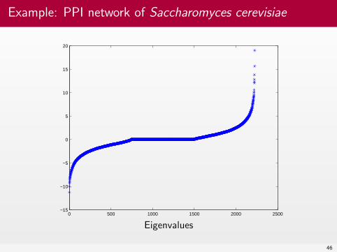
Example: PPI network of Saccharomyces cerevisiae
0 500 1000 1500 2000 2500−15
−10
−5
0
5
10
15
20
Eigenvalues
46

Example: Intravenous drug users network
0 100 200 300 400 500 600
0
100
200
300
400
500
600
nz = 4024
Adjacency matrix, |V | = 616, |E| = 2012.
47

Example: Intravenous drug users network
0 100 200 300 400 500 600
0
100
200
300
400
500
600
nz = 4024
Same, reordered with Reverse Cuthill–McKee
48

Example: Intravenous drug users network
0 10 20 30 40 50 600
50
100
150
200
250
Degree distribution (dmin = 1, dmax = 58)
49

Example: Intravenous drug users network
0 100 200 300 400 500 600 700−10
−5
0
5
10
15
20
Eigenvalues
50

Graph Laplacian spectra
For an undirected network, the spectrum of the graph LaplacianL = D −A also plays an important role. For instance, the connectivityproperties of G can be characterized in terms of spectral properties of L;moreover, L plays an important role in the study of diffusion processes onG.
The eigenvalues of L are all real and nonnegative, and since L1 = 0,where 1 denotes the vector of all ones, L is singular. Hence, 0 ∈ σ(L).The graph Laplacian L is a singular M -matrix.
Theorem. The multiplicity of 0 as an eigenvalue of L coincides with thenumber of connected components of the network.
Corollary. For a connected network, the null space of the graph Laplacianis 1-dimensional and is spanned by 1. Thus, rank(L) = N − 1.
51

Graph Laplacian spectra (cont.)
Let G be a simple, connected graph.
The eigenvector of L associated with the smallest nonzero eigenvalue iscalled the Fiedler vector of the network. Since this eigenvector must beorthogonal to the vector of all ones, it must contain both positive andnegative entries.
There exist elegant graph partitioning algorithms that assign nodes todifferent subgraphs based on the sign of the entries of the Fiedler vector.
These methods, however, tend to work well only in the case of fairly regulargraphs, such as those arising from the discretization of PDEs. In general,partitioning complex graphs (scale-free graphs in particular) is very hard!
52

Graph Laplacian spectra (cont.)
If the graph G is regular, then D = dIN −A, therefore the eigenvalues ofthe Laplacian are just
λi(L) = d− λi(A), 1 ≤ i ≤ N .
If G is not a regular graph, there is no simple relationship between theeigenvalues of L and those of A.
Also useful is the notion of normalized Laplacian:
L̂ := IN −D−1/2AD−1/2 .
In the case of directed graphs, there are several distinct notions of graphLaplacian in the literature.
53

Example: PPI network of Saccharomyces cerevisiae
Laplacian eigenvalues (λ2(L) = 0.0600, λN (L) = 65.6077)54

Example: Intravenous drug users network
Laplacian eigenvalues (λ2(L) = 0.0111, λN (L) = 59.1729)55

Outline
1 Complex networks: motivation and background
2 Network structure: centrality and communicability measures
3 Bibliography
56

Centrality measures
There are dozens of different definitions of centrality for nodes in a graph.The simplest is degree centrality, which is just the degree di of node i.This does not take into account the “importance” of the nodes a givennodes is connected to—only their number.
A popular notion of centrality is betweenness centrality (Freeman, 1977),defined for any node i ∈ V as
CB(i) :=∑j 6=i
∑k 6=i
δjk(i) ,
where δjk(i) is the fraction of all shortest paths in the graph betweennodes j and k which contain node i:
δjk(i) :=# of shortest paths between j, k containing i
# of shortest paths between j, k.
57

Centrality measures (cont.)
The degree is very cheap to compute but is unable to recognize thecentrality of certain nodes: it’s a purely local notion.
58

Centrality measures (cont.)
Another centrality measure popular in social network analysis is closenesscentrality (Freeman, 1979), defined as
CC(i) =1∑
j∈V d(i, j).
Betweenness and closeness centrality assume that all communication inthe network takes place via shortest paths, but this is often not the case.
This observation has motivated a number of alternative definitions ofcentrality, which aim at taking into account the global structure of thenetwork and the fact that all walks between pairs of nodes should beconsidered, not just shortest paths.
59
Centrality measures (cont.)
We mention here that for directed graphs it is often necessary todistinguish between hubs and authorities. Indeed, in a directed graph anode plays two roles: broadcaster and receiver of information.
Crude broadcast and receive centrality measures are provided by theout-degree dout
i and by the in-degree dini of the node, respectively.
Other, more refined receive and broadcast centrality measures will beintroduced later.
60

Spectral centrality measures
Bonacich’s eigenvector centrality (1987) uses the entries of the dominanteigenvector x to rank the nodes in the network in order of importance: thelarger xi is, the more important node i is considered to be. By thePerron–Frobenius Theorem, the vector x is positive and unique providedthe network is connected.
The underlying idea is that “a node is important if it is linked to many importantnodes.” This circular definition corresponds to the fixed-point iteration
x(k+1) = Ax(k), k = 0, 1, . . .
which converges, upon normalization, to the dominant eigenvector of A ask →∞. The rate of convergence depends on the spectral gap γ = λ1 − λ2. Thelarger γ, the faster the convergence.
In the case of directed networks, the dominant left and right eigenvectors of Aprovide authority and hub scores, respectively.
61

Spectral centrality measures (cont.)
Google’s PageRank algorithm (Brin & Page, 1998) is a variant ofeigenvector centrality, applied to the (directed) graph representing webpages (documents), with hyperlinks between pages playing the role ofdirected edges. Since the WWW graph is not connected, some tweaks (inthe form of a rank-one modification to the hyperlink matrix) are needed tohave a unique PageRank eigenvector.
PageRank has a probabilistic interpretation in terms of random walks onthe web graph, a special type of Markov chain. The PageRank eigenvectoris the stationary probability distribution of this Markov chain.
An alternative approach (HITS), proposed by J. Kleinberg in 1998, uses thedominant left and right singular vectors of the (nonsymmetric) adjacency matrixof the graph in order to obtain both hub and authority scores. We will return tothis topic in Lecture III.
62

Subgraph centrality
We now turn to centrality measures that are based on matrix functions.
Subgraph centrality (Estrada & Rodríguez-Velásquez, Phys. Rev. E, 2005)measures the centrality of a node by taking into account the number ofsubgraphs the node “participates” in.
This is done by counting, for all k = 1, 2, . . . the number of closed walks inG starting and ending at node i, with longer walks being penalized (givena smaller weight).
It is sometimes useful to introduce a tuning parameter β > 0 (“inversetemperature") to simulate external influences on the network, for example,increased tension in a social network, financial distress in the bankingsystem, etc.
63

Subgraph centrality (cont.)
Recall that
(Ak)ii = # of closed walks of length k based at node i,(Ak)ij = # of walks of length k that connect nodes i and j.
Using βk/k! as weights leads to the notion of subgraph centrality:
SC(i) =
[I + βA +
β2
2!A2 +
β3
3!A3 + · · ·
]ii
= [eβA]ii .
Note that SC(i) ≥ 1. Subgraph centrality has been used successfully invarious settings, including proteomics and neuroscience.
Note: the weights are needed to “penalize" longer walks, and to make the powerseries converge.
64

Subgraph centrality (cont.)
It is sometimes desirable to normalize the subgraph centrality of a node bythe sum
EE(G, β) =N∑
i=1
SC(i) =N∑
i=1
[eβA]ii = Tr(eβA) =N∑
i=1
eβλi
of all the subgraph centralities. The quantity EE(G, β) is known as theEstrada index of the graph G.
It is analogous to the partition function Z in statistical physics, and itplays an important role in the statistical mechanics of complex networks.
65

Subgraph centrality (cont.)
Note that the normalized subgraph centralities define a probabilitydistribution p(i) := SC(i)/EE(G) on the set V of nodes.
Analogous to the Gibbs–Shannon entropy, one can then define the walkentropy of a graph G by
S(G, β) := −N∑
i=1
p(i) log2 p(i) .
The walk entropy provides a useful measure of the complexity of a graph(Estrada, de la Peña, & Hatano, Lin. Algebra Appl., 2014.)
66

Subgraph centrality (cont.)
Other matrix functions of interest in network analysis are cosh(A) andsinh(A), which correspond to considering only walks of even and oddlength, respectively.
In a bipartite graph there cannot be any closed walks of odd length; hence,all the diagonal entries of A2k+1 must be zero, for all k ≥ 0. ThereforeTr (sinh(A)) = 0. Hence, the quantity
B(G) :=Tr (cosh(A))
Tr (eA)
provides a measure of how “close” a given graph is to being bipartite: ifB(G) is close to 1, then G is “nearly bipartite".
Hyperbolic matrix functions are also used to define the notion of returnability indigraphs (E. Estrada & N. Hatano, Lin. Algebra Appl., 2009).
67

Katz centrality
Of course different weights can be used, leading to different matrix functions,such as the resolvent (Katz, 1953):
(I − αA)−1 = I + αA + α2A2 + · · · =∞∑
k=0
αkAk, 0 < α < 1/λ1.
Note that I − αA is a nonsingular M -matrix, in particular (I − αA)−1 ≥ 0.
Originally, Katz proposed to use the row sums of (I − αA)−1 as a centralitymeasure:
CK(i) = eTi (I − αA)−11 .
Resolvent-based subgraph centrality uses instead the diagonal entries of(I − αA)−1 (E. Estrada & D. Higham, SIAM Rev., 2010).
In the case of a directed network one can use the solution vectors of the linearsystems
(I − αA)x = 1 and (I − αAT )y = 1
to rank hubs and authorities. These are the row and column sums of the matrixresolvent (I − αA)−1, respectively.
68

Comparing centrality measures
Different centrality measures correspond to different notions of what itmeans for a node to be “influential"; some (like degree) only look at localinfluence, others (like eigenvector centrality and PageRank) emphasizelong distance influences, and others (like subgraph and Katz centrality) tryto take into account short, medium and long range influences.
Others yet, like closeness and betweenness centrality, emphasize nodesthat are a short distance away from most other nodes, or that are centralto the flow of information along shortest paths in G.
And these are just a few of the many centrality measures proposed in theliterature!
69

Comparing centrality measures (cont.)
A natural question at this point is: which centrality measure is better?Which measure should be used?
Unfortunately, it is not possible to give a general, satisfactory answer tothis question. Some centrality measures may work very well on a networkand not so well on others.
Competing methods can be tested on networks for which some kind ofground truth is known, for example, from experiments (e.g., PPI networkof yeast), and the “best one" can then be used on similar networks, butwith few guarantees of success.
Often, however, multiple centrality measures are used and one looks at theoverlap between lists of top-ranked nodes (a form of consensus).
70

Comparing centrality measures (cont.)
Some centrality measures have been shown to have greater discriminatingpower than others.
For example, if a graph G is regular (di = d for all i = 1 : N), degreecentrality, eigenvector centrality and Katz centrality (as well as all othercentrality measures of the form c = f(A)1) are unable to distinguishbetween the nodes in G: all nodes are given equal status.
In contrast, there are regular graphs for which subgraph centrality is ableto identify nodes than are more “central" than others.
Hence, subgraph centrality has a higher discriminating power than othercentrality measures.
A recent result of Estrada and de la Peña (LAA, 2014) states that in a graph G
all nodes have the same subgraph centrality ([eA]ii = const.) if and only if G iswalk regular, i.e., [Ak]ii = c(k) = const. (independent of i) for all k = 0, 1, . . ..
71

Comparing centrality measures (cont.)
4
2
3
1
6
7
5
8
Figure: A 3-regular graph on 8 nodes which is not walk-regular.
Example of a 3-regular graph on 8 nodes for which subgraph centrality candiscriminate among nodes. Node 4 has the highest subgraph centrality, node 5the lowest.
72

Comparing centrality measures (cont.)
In the case of very large-scale networks (with millions or even billions ofnodes/edges), computational cost becomes a limiting factor.
Of course, degree centrality is very cheap, but as we know it is not verysatisfactory.
At the other end of the spectrum, subgraph centrality (which scalesroughly like O(N2)) is very satisfactory but is too expensive for verylarge networks.
For large networks, methods like eigenvector and Katz centrality, whilestill potentially expensive, are often used, together with closeness andbetweenness centrality.
73

Comparing centrality measures (cont.)
In practice, one often finds a good degree of correlation between therankings provided by (apparently very different) centrality measures.How can we explain this?
Suppose A is the adjacency matrix of an undirected, connected network.Let λ1 > λ2 ≥ λ3 ≥ . . . ≥ λN be the eigenvalues of A, and let xk be anormalized eigenvector corresponding to λk. Then
eβA =N∑
k=1
eβλkxkxTk
and therefore
SC(i) =N∑
k=1
eβλkx2k,i ,
where xk,i denotes the ith entry of xk.
Similar spectral formulas exist for other centrality measures based on matrixfunctions (e.g., the resolvent).
74

Comparing centrality measures (cont.)
Dividing all the subgraph centralities by eβλ1 has no effect on the centralityrankings:
e−βλ1 [eβA]ii = x21,i +
N∑k=2
eβ(λk−λ1)x2k,i .
It is clear that when the spectral gap is sufficiently large (λ1 � λ2), the centralityranking is essentially determined by the dominant eigenvector x1, since thecontributions to the centrality scores from the remaining eigenvalues/vectorsbecomes negligible, in relative terms.
The same is true if β is chosen “large".
Hence, in this case subgraph centrality can be expected to give similar results toeigenvector centrality. The same applies to Katz centrality.
In contrast, the various measures can give significantly different results when thespectral gap is small. In this case, going beyond the dominant eigenvector canresult in significant differences in the corresponding rankings.
75

Comparing centrality measures (cont.)
Theorem: Let A be the adjacency matrix for a simple, connected,undirected graph G. Then
For α → 0+, Katz centrality reduces to degree centrality;For α → 1
λ1−, Katz centrality reduces to eigenvector centrality;
For β → 0+, subgraph centrality reduces to degree centrality;For β →∞, subgraph centrality reduces to eigenvector centrality.
Note: A similar result holds for directed networks, in which case we needto distinguish between in-degree, out-degree, left/right dominanteigenvectors, and row/column sums of (I − αA)−1 and eβA.
M. Benzi & C. Klymko, A matrix analysis of different centrality measures,submitted (2014).
76

Comparing centrality measures (cont.)
The previous result helps explain why Katz and subgraph centrality aremost informative and useful when the parameters α, β are chosen to beneither too small, nor too large.
In practice, we found that a good choice for Katz’s parameter is α = δ/λ1,with 0.5 ≤ δ ≤ 0.9; for subgraph centrality it is best to use 0.5 ≤ β ≤ 2.
As default parameters we recommend α = 0.85/λ1 and β = 1, althoughsmaller values should be used for networks with large spectral gapγ = λ1 − λ2.
77

Communicability
Communicability measures how “easy” it is to send a message from node ito node j in a graph. It is defined as (Estrada & Hatano, 2008):
C(i, j) = [eβA]ij
=
[I + βA +
β2
2!A2 +
β3
3!A3 + · · ·
]ij
≈ weighted sum of walks joining nodes i and j.
Note that as the temperature increases (β → 0) the communicabilitybetween nodes decreases (eβA → I).
Communicability has been successfully used to identify bottlenecks in networks(e.g., regions of low communicability in brain networks) and for communitydetection.
E. Estrada & N. Hatano, Phys. Rev. E, 77 (2008), 036111;E. Estrada, N. Hatano, & M. Benzi, Phys. Rep., 514 (2012), 89–119.
78

Communicability (cont.)
The total communicability of a node is defined as
TC(i) :=N∑
j=1
C(i, j) =N∑
j=1
[eβA]ij .
This is another node centrality measure that can be computed veryefficiently, even for large graphs, since it involves computing eβA 1 andKrylov methods are very good at this!
79

Communicability (cont.)
The normalized total communicability of G:
TC(G) :=1
N
N∑i=1
N∑j=1
C(i, j) =1
N1T eβA 1
provides a global measure of how “well-connected" a network is, and canbe used to compare different network designs.
Thus, highly connected networks, such as small-world networks withoutbottlenecks, can be expected to have a high total communicability.
Conversely, large-diameter networks with a high degree of locality (such asregular grids, road networks, etc.) or networks containing bottlenecks arelikely to display a low value of TC(G).
80

Global communicability measures (cont.)
Note that TC(G) can be easily bounded from below and from above:
1
NEE(G) ≤ TC(G) ≤ eβλ1
where EE(G) = Tr(eβA) is the Estrada index of the graph. These boundsare sharp, as can be seen from trivial examples.
In the next Table we present the results of some calculations (for β = 1) ofthe normalized Estrada index, global communicability and eλ1 for variousreal-world networks.
M. Benzi & C. F. Klymko, J. Complex Networks, 1 (2013), 124–149.
81

Communicability (cont.)
Table: Comparison of the normalized Estrada index E(G) = Tr(eA)/N , thenormalized total network communicability TC(G), and eλ1 for various real-worldnetworks.
Network E(G) TC(G) eλ1
Zachary Karate Club 30.62 608.79 833.81Drug User 1.12e05 1.15e07 6.63e07Yeast PPI 1.37e05 3.97e07 2.90e08
Pajek/Erdos971 3.84e04 4.20e06 1.81e07Pajek/Erdos972 408.23 1.53e05 1.88e06Pajek/Erdos982 538.58 2.07e05 2.73e06Pajek/Erdos992 678.87 2.50e05 3.73e06SNAP/ca-GrQc 1.24e16 8.80e17 6.47e19
SNAP/ca-HepTh 3.05e09 1.06e11 3.01e13SNAP/as-735 3.00e16 3.64e19 2.32e20
Gleich/Minnesota 2.86 14.13 35.34
82

Communicability (cont.)
Communicability and centrality measures can also be defined using thenegative graph Laplacian −L = −D + A instead of the adjacency matrixA.
When the graph is regular (the nodes have all the same degree d, henceD = dI) nothing is gained by using −L instead of A, owing to the obviousidentity
e−L = e−dI+A = e−deA.
Most real networks, however, have highly skewed degree distributions, andusing e−L instead of eA can lead to substantial differences. Note that theinterpretation in terms of weighted walks is no longer valid in this case.
Laplacian-based centrality and communicability measures are especiallyuseful in the study of dynamic processes on graphs.
83

Outline
1 Complex networks: motivation and background
2 Network structure: centrality and communicability measures
3 Bibliography
84

Monographs
U. Brandes and T. Erlebach (Eds.), Network Analysis.Methodological Foundations, Springer, LNCS 3418, 2005.F. Chung and L. Lu, Complex Graphs and Networks, AmericanMathematical Society, 2006.A. Barrat, M. Barthelemy, and A. Vespignani, Dynamical Processeson Complex Networks, Cambridge University Press, 2008.M. E. J. Newman, Networks. An Introduction, Oxford UniversityPress, 2010.P. Van Mieghem, Graph Spectra for Complex Networks, CambridgeUniversity Press, 2011.E. Estrada, The Structure of Complex Networks, Oxford UniversityPress, 2011.Excellent accounts by Barabási (2002) e Watts (2003) for a generalreadership.
85

Specialized journals
Two new journals launched in 2013:
Journal of Complex Networks (Oxford University Press)
Network Science (Cambridge University Press)
http://comnet.oxfordjournals.org/
http://journals.cambridge.org/action/displayjournal?jid=NWS
86