Lecture 9: Theories of the Yield Curve. Lecture 9: …pages.stern.nyu.edu/~alynch/courses/B01.231160/ff06S09.pdfLecture 9 Foundations of Finance 5 D. Examples: 1. U.S. 04/2004: slope

Lecture 9 Foundations of Finance

0

Lecture 9: Theories of the Yield Curve.

I. Reading.II. Expectations HypothesisIII. Liquidity Preference Theory.IV. Preferred Habitat Theory.

Lecture 9: Bond Portfolio Management.

V. Reading.VI. Risks associated with Fixed Income Investments.VII. Duration.VIII. Immunization.

Lecture 9-10: Derivatives: Definitions and Payoffs.

IX. Readings.X. Preliminaries.XI. Options.XII. Forward and Futures Contracts.XIII. Features of Derivatives.XIV. Motives for Holding Derivatives.


1

Lecture 9: Theories of the Yield Curve.

I. Reading.A. BKM, Chapter 15.3-15.4.


2

II. Expectations HypothesisA. Setting:

1. Individuals do not care about interest rate risk.2. So expected return over any future period is the same for all discount

bonds and forward contracts.

B. Statements of the expectations hypothesis: 3 approximately equivalent (if usingcontinuously compounded rates then the 3 are exactly equivalent)1. The yield on an n-year discount bond is equal to the geometric average of

the expected ½-year spot rates for the next n years:

(1 %yn(0)

2) ' (1 %

y½(0)2

) (1 %Eat time 0[y½(½)]

2)... (1 %

Eat time 0[y½(n&½)]2

)1

2n

2. Expected return over the next ½-year on a discount bond of any maturityis equal to the ½-year spot rate:

y½(0) = Eat time 0[hn(½)] for any n,

where hn(½) is the return on a discount bond with a maturity n years in thefuture for the ½-year ending at time ½..

3. Forward rate available today for any future ½-year period is equal to theexpected future spot rate for that period:

fn,n+½(0) = Eat time 0[y½(n)] for any n.

C. Implications:1. Yield curve slope and expectations about future spot rates:

a. Upward sloping yield curve implies an expectation of higher spotrates in the future.

b. Downward sloping yield curve implies an expectation of lowerspot rates in the future.

2. Yield curve slope and expectations about future economic activity:a. A very positive slope is expected to predicts strong future GDP

growth: Low short-term interest rates generate much investmenttoday which in turn creates an expectation of strong future GDPgrowth.

b. Empirically:(1) the slope of the yield curve is one of the best available

predictors for the growth rate of the economy.(2) a very positive slope predicts strong future GDP growth.


3


4


5

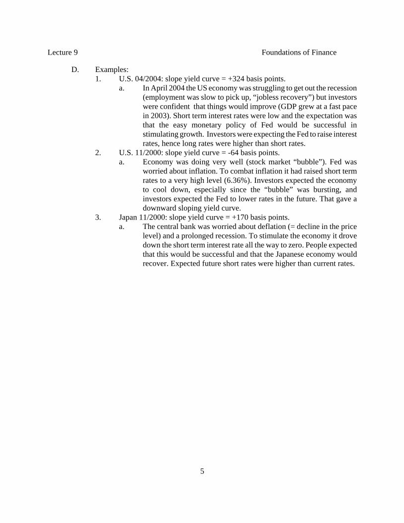
D. Examples:1. U.S. 04/2004: slope yield curve = +324 basis points.

a. In April 2004 the US economy was struggling to get out the recession(employment was slow to pick up, “jobless recovery”) but investorswere confident that things would improve (GDP grew at a fast pacein 2003). Short term interest rates were low and the expectation wasthat the easy monetary policy of Fed would be successful instimulating growth. Investors were expecting the Fed to raise interestrates, hence long rates were higher than short rates.

2. U.S. 11/2000: slope yield curve = -64 basis points.a. Economy was doing very well (stock market “bubble”). Fed was

worried about inflation. To combat inflation it had raised short termrates to a very high level (6.36%). Investors expected the economyto cool down, especially since the “bubble” was bursting, andinvestors expected the Fed to lower rates in the future. That gave adownward sloping yield curve.

3. Japan 11/2000: slope yield curve = +170 basis points.a. The central bank was worried about deflation (= decline in the price

level) and a prolonged recession. To stimulate the economy it drovedown the short term interest rate all the way to zero. People expectedthat this would be successful and that the Japanese economy wouldrecover. Expected future short rates were higher than current rates.


6

4. U.S. 06/2005: slope yield curve = +140 basis points.a. Market expected future spot rates to be higher: a year later, the yield

curve has shifted up, suggesting that the market’s expectation ofhigher future spot rates was realized.


7

b. Upward sloping yield curve suggests strong future GDP growth canbe expected: GDP growth in the first quarter of 2006 was strongestsince the third quarter of 2003.

5. U.S. 06/2006: yield curve flat at around 5%a. Suggests that market is expecting future spot rates to remain at 5%

into the future.b. Suggests that future GDP growth not expected to be high.


8

III. Liquidity Preference Theory.A. Setting:

1. Individuals require a liquidity premium to hold less liquid, longer maturitybonds: there is an associated price discount.

2. The percentage change in the associated price discount going to the nextlongest maturity is always positive.

B. Statement: 1. The yield on an n-year discount bond is always higher than the geometric

average of the expected ½-year spot rates for the next n years:

(1 %yn(0)

2) ' b½(0) b1(0)...bn(0)

12n

(1 %y½(0)

2) (1 %

Eat time 0[y½(½)]2

)... (1 %Eat time 0[y½(n&½)]

2)

12n

where b½ = 1 and the theory says bt>1 for all t>½.C. Implications:

1. More likely to see upward-sloping yield curves.2. Forward rates are upward biased predictors of future ½-year spot rates:

fn,n+½(0) > Eat time 0[y½(n)] for all n>½.

3. Yield curve slope and expectations about future spot rates:a. Upward sloping yield curve is consistent with the market expecting

higher or lower spot rates in the future. b. Downward sloping yield curve implies that the market is expecting

lower spot rates in the future.

IV. Preferred Habitat Theory.A. Setting:

1. Yields on different securities are determined by the supply and demand forthat security.

2. Securities with similar maturities may not be close substitutes.B. Statement:

1. The yield on an n-year discount bond can be higher or lower than thegeometric average of the expected ½-year spot rates for the next n years: bt>1or <1 for all t>½..

C. Implications: Slope of the yield curve tells you little about whether the market isexpecting higher or lower spot rates in the future.


9


9

Lecture 9: Bond Portfolio Management.

I. Reading.A. BKM, Chapter 16, Sections 16.1 and 16.3.

II. Risks associated with Fixed Income Investments.A. Reinvestment Risk.

1. If an individual has a particular time horizon T and holds an instrumentwith a fixed cash flow received prior to T, then the investor facesuncertainty about what yields will prevail at the time of the cash flow. This uncertainty is known as reinvestment risk.

2. Example: Suppose an investor has to meet a obligation of $5M in twoyears time. If she buys a two year coupon bond to meet this obligation,there is uncertainty about the rate at which the coupons on the bond can beinvested. This uncertainty is an example of reinvestment risk.

B. Liquidation Risk. 1. If an individual has a particular time horizon T and holds an instrument

which generates cash flows that are received after T, then the investorfaces uncertainty about the price of the instrument at time T. Thisuncertainty is known as liquidation risk.

2. Example: Suppose an investor has to meet a obligation of $5M in twoyears time. If she buys a five year discount bond to meet this obligation,there is uncertainty about the price at which this bond will sell in twoyears time. This uncertainty is an example of liquidation risk.


10

III. Duration.A. Definition.

1. Macaulay Duration.a. Let 1 period=1 year.b. Consider a fixed income instrument i which generates the

following stream of certain cash flows: 0 ½ 1 1½ 2 2½ N-½ N .)))))))))2)))))))))2)))))))))2)))))))))2)))))))))2)) ... ))2)))))))))-

Ci(½) Ci(1) Ci(1½) Ci(2) Ci(2½) Ci(N-½) Ci(N)

Let yi(0) be the YTM at time 0 on the instrument expressed as an APRwith semi-annual compounding.c. Macaulay duration is defined as

D i(0) ' ½ k i(½) % 1 k i(1) %1½ k i(1½) %... % N k i(N)

where .k i(t) '1

P i(0)C i(t)

[1%y i(0)/2]2t

d. Note that the ki(t)s sum to 1:

.1 ' k i(½) % k i(1) % k i(1½) %... % k i(N)

2. “Modified” Duration.a. “Modified” duration D*i(0) is defined to be Macaulay duration

divided by [1+yi(0)/2]:

D*i(0) = Di(0) /[1+yi(0)/2].

b. “Modified” duration is often used in the industry.


11

3. Example. 2/15/06. The 3 Feb 07 note has a price of 97.1298 and a YTMexpressed as an APR with semi-annual compounding of 6%. a. Its k’s can be calculated:

k3 Feb 07(½) = (1.5/1.03)/97.1298 = 1.4563/97.1298 = 0.0150.k3 Feb 07(1) = (101.5/1.032)/97.1298 = 95.6735/97.1298 = 0.9850.

b. Its duration can be calculated:

D3 Feb 07(0) = ½ x k3 Feb 07(½) + 1 x k3 Feb 07(1)= ½ x 0.0150 + 1 x 0.9850 = 0.9925 years.

c. Its modified duration can be calculated:

D* 3 Feb 07(0) = 0.9925 /(1+0.03) = 0.9636.


12

B. Duration can be interpreted as the effective maturity of the instrument.1. If the instrument is a zero coupon bond, then its duration is equal to the

time until maturity.2. For an instrument with cash flows prior to maturity, its duration is less

than the time until maturity.3. Holding maturity and YTM constant, the larger the earlier payments

relative to the later payments then the shorter the duration. 4. Example: 2/15/06. Suppose the 10 Feb 07 coupon bond has a price of

103.8270 and a YTM expressed as an APR with semi-annualcompounding of 6%. a. Its k’s can be calculated:

k10 Feb 07(½) = (5/1.03)/103.8270 = 4.8544/103.8270 = 0.0468.k10 Feb 07(1) = (105/1.032)/103.8270 = 98.9726/103.8270 = 0.9532.

b. Its duration can be calculated:D10 Feb 07(0) = ½ x k10 Feb 07(½) + 1 x k10 Feb 07(1) = ½ x 0.0468 + 1 x 0.9532 = 0.9766 years.

c. So the 10 Feb 07 bond with larger earlier cash flows relative tolater cash flows has a shorter duration than the 3 Feb 07 bond.

C. Duration of a Portfolio.1. If a portfolio C has ωA,C invested in asset A at time 0 and ωB,C invested in

asset B at time 0 and the YTMs of A and B are the same, the duration of Cis given by:

.D C(0) ' ωA,C D A(0) % ωB,C D B(0)

2. Example (cont): 2/15/06. Suppose Tom forms a portfolio on 2/15/06 with40% in 3 Feb 07 coupon bonds and the rest in 10 Feb 07 coupon bonds. a. The portfolio’s duration can be calculated:

DP(0) = ω3 Feb 07,P D 3 Feb 07(0) + ω10 Feb 07,P D 10 Feb 07(0)= 0.4 x 0.9925 + (1-0.4) x 0.9766 = 0.98296.

Instrument YTM(2/15/06) Duration(2/15/06)

Feb 07 Strip 6% 1.0000

3 Feb 07 Bond 6% 0.9925

10 Feb 07 Bond 6% 0.9766

40% of 3 Feb 07 and 60% of 10 Feb 07

6%6%

0.9925 x 0.4 +0.9766 x 0.6 = 0.98296


13

D. Duration as a measure of yield sensitivity.1. The price of bond i described above is given by:

.P i(0) 'C i(½)

[1%y i(0)/2]1%

C i(1)[1%y i(0)/2]2

%C i(1½)

[1%y i(0)/2]3%...% C i(N)

[1%y i(0)/2]2N

2. To assess the impact of the price of bond i to a shift in yi(0), differentiatethe above expression with respect to yi(0):d P i(0)

d y i(0)

' & ½ C i(½)[1%y i(0)/2]2

& 1 C i(1)[1%y i(0)/2]3

& 1½ C i(1½)[1%y i(0)/2]4

&...& N C i(N)[1%y i(0)/2]2N%1

3. Thus, bond i’s modified Macaulay duration is related to the sensitivity ofits price to shifts in yi(0) as follows:

.d P i(0)d y i(0)

' &P i(0) D (i(0)

4. Thus, bond i’s modified Macaulay duration measures its price sensitivityto a change in its yield (where price sensitivity is measured by thepercentage change in the price).

5. In particular, a small change in yi(0), ∆yi(0), causes a change in Pi(0),∆Pi(0), which satisfies:

.∆ P i(0) . &P i(0) D (i(0) ∆y i(0)

6. For coupon bonds and strips, price is a convex function of yield: so theduration-based price-change approximation overstates the price declinewhen the YTM increases and understates the price increase when theYTM decreases.


14

7. Example (cont): 2/15/06. The 3 Feb 07 note has a price of 97.1298 and aYTM expressed as an APR with semi-annual compounding of 6%. a. Using the formula for approximate price change involving

modified duration above:

YTM increase: ∆P3 Feb 07(0) = -97.1298 x 0.9636 x 0.01 = -0.9359.YTM decrease: ∆P3 Feb 07(0) = -97.1298 x 0.9636 x -0.01 = 0.9359.

b. Can compare the approximate price changes to the actual pricechanges:

3 Feb 07

YTM P(0) Actual ∆P(0) YTM = 6% ∆YTM Approx ∆P(0) = -P(0)D*(0)∆YTM

P(0) D*(0)

7% 96.2006 -0.929297.1298 0.9636

+0.01 -0.9359

6% 97.1298 0 0 0

5% 98.0725 +0.9427 -0.01 +0.9359


15


16

IV. Immunization.A. Dedication Strategies.

1. A dedication strategy ensures that a stream of liabilities can be met fromavailable assets by holding a portfolio of fixed income assets whose cashflows exactly match the stream of fixed outflows.

2. Note that both the asset portfolio and the liability stream have the samecurrent value and duration.

3. Example: It is 2/15/06 and QX must pay $5M on 8/15/06 and $10M on2/15/07. A dedication strategy would involve buying Aug 06 U.S. stripswith a face value of $5M and Feb 07 U.S. strips with a face value of$10M.

B. Target Date Immunization.1. Assumptions.

a. the yield curve is flat at y (APR with semiannual compounding).b. any shift in the curve keeps it flat.

2. Target date immunization ensures that a stream of fixed outflows can bemet from available assets by holding a portfolio of fixed income assets:a. with the same current value as the liability stream; and,b. with the same modified duration.

3. Note:a. given the flat yield curve, all bonds have the same YTM, y.b. for this reason, a small shift in the yield curve will have the same

effect on the value of the immunizing assets and on the value ofthe liabilities (using the definition of duration).

c. and so, the assets will still be sufficient to meet the stream of fixedoutflows.

d. further, it is easy to work out the current value of the liabilitystream using y.

e. equating the modified durations of the assets and the liabilities isthe same as equating the durations.


17

4. Example: Firm GF is required to make a $5M payment in 1 year and a$4M payment in 3 years. The yield curve is flat at 10% APR with semi-annual compounding. Firm GF wants to form a portfolio using 1-year and4-year U.S. strips to fund the payments. How much of each strip must theportfolio contain for it to still be able to fund the payments after a shift inthe yield curve?a. The value of the liabilities is given by:

L(0) = 5M/[1+0.1/2]2 + 4M/[1+0.1/2]6 = 4.5351M + 2.9849M = 7.5200M.

b. The duration of the liabilities is given by:

DL(0) = 1 x [4.5351/7.5200] + 3 x [2.9849/7.5200] = 1.7938 years.

c. Let A1(0) be the portfolio’s dollar investment in the 1-year stripsand A4(0) be the portfolio’s dollar investment in the 4-year strips.

d. The dollar value of the portfolio must equal the value of theliabilities. So A1(0) + A4(0) = 7.5200M.

e. The duration of the portfolio equals

DP(0) = ω1,P D1(0) +(1-ω1,P) D4(0)

where ω1,P = A1(0)/ 7.5200M. The duration of the 1-year strip is 1and the duration of the 4-year strip is 4.

f. Setting the duration of the portfolio equal to the duration of theliabilities gives:

1.7938 = ω1,P D1(0) +(1-ω1,P) D4(0) = ω1,P 1 +(1-ω1,P) 4 Y ω1,P = 0.7354.

g. Thus,

A1(0) = 0.7354 x 7.5200M = 5.5302M; and, A4(0) = 7.5200M - 5.5302M = 1.9898M.


18

5. Generalizations.a. The assumption of a flat yield curve has undesirable properties.b. When the yield curve is allowed to take more general shapes,

target-date immunization is still possible, but modified Macaulayduration is not appropriate for measuring the impact of a yieldcurve shift on price. Need to use a more general duration measure.

C. Comparison.1. Dedication strategies are a particular type of target date immunization.2. The one advantage of a dedication strategy is that there is no need to

rebalance through time. Almost all other immunization strategies involvereimmunizing over time.

Lecture 9-10 Foundations of Finance

19

Lecture 9-10: Derivatives: Definitions and Payoffs.

I. Readings.A. Options:

1. BKM, Chapter 20, Sections 20.1 - 20.4.B. Forward and Futures Contracts.

1. BKM, Chapter 22, Sections 22.1 - 22.3.

II. Preliminaries.A. Payoff Diagrams.

1. Let S(t) be the value of one unit of an asset at time t.2. Payoff diagram graphs the value of a portfolio at time T as a function of

S(T).3. Long 1 unit of the asset is represented by a 45E line through the origin.4. Short 1 unit of the asset is represented by a -45E line through the origin.5. Long a discount bond with a face value of $50 maturing at T is

represented by a horizontal line at $50: its value at T is $50 irrespective ofthe value of the asset.

6. Short a discount bond with a face value of $50 maturing at T isrepresented by a horizontal line at -$50.


20


21


22


23


24

III. Options.A. Call Option.

1. Definition.a. A call option gives its holder the right (but not the obligation) to

buy the option’s underlying asset at a specified price.b. The specified price is known as the exercise or strike price.c. A European option can only be exercised at the expiration date of

the option. An American option can be exercised any time prior tothe expiration of the option.

Position opened at time 0 Time 0 Time T

S(T)<50 S(T)$50

Long 1 European Call Option on the Stockexpiring at T with an exercise price of $50

-C50,T(0) 0 S(T)-50 max [S(T)-50,0]


25

2. Payoff at the Expiration Date to the Holder of a European Option.a. Let T be the expiration date, X=$50 be the strike price and S(t) be

the value of the option’s underlying asset at time t.b. Since the holder of the option is not obligated to buy the asset for

$50, she will only do so when the payoff from doing so is greaterthan zero.(1) The price paid by the holder prior to T for the option is

irrelevant to the decision to exercise since it is a sunk cost.(2) If [S(T)-50] > 0, the holder wants to exercise the option as

it allows her to buy for $50 an asset worth more than $50.(3) If [S(T)-50] < 0, the holder does not want to exercise the

option since she would be paying $50 for an asset she couldbuy in the market for less than $50. So her payoff is zero.

(4) Thus, the holder’s payoff from the call option is max{S(T)-50, 0}.

(5) Since the payoff from the option is non-negative, noarbitrage tells you that the call option has a non-negativevalue at any time t, C50(t), prior to T.

(6) At the expiration date, C50(T) = max {S(T)-50, 0}.


26

3. Writer of the Call Option.a. The payoff to the option writer is just the negative of the payoff to

the option holder.b. In return, the option writer receives the option’s value when she

first writes the call option and sells it.c. Suppose the call is written at time 0 and both the writer and the

option buyer keep their positions until expiration. Can see that thesum of the writer’s and the holder’s payoff is zero.


S(T)<50 S(T)$50

Long 1 European Call Option on the Stockexpiring at T with an exercise price of $50

-C50,T(0) 0 S(T)-50 max [S(T)-50,0]

Short 1 European Call Option on the Stockexpiring at T with an exercise price of $50

C50,T(0) 0 -[S(T)-50] -max [S(T)-50,0]

Sum 0 0 0 0


27


28

d. If the option holder exercises the option, the option writer must sellthe asset to the holder for $50. Her payoff is -[S(T)-50].

e. If the option holder does not exercise the option, the writer is notobliged to do anything. Her payoff is 0.


29

B. Put Option.1. Definition.

a. A put option gives its holder the right (but not the obligation) tosell the option’s underlying asset at a specified price (also calledthe exercise or strike price).

b. European and American have the same connotations for puts as forcalls.


S(T)<50 S(T)$50

Long 1 European Put Option on the Stockexpiring at T with an exercise price of $50

-P50,T(0) 50-S(T) 0 max [50-S(T),0]

2. Payoff at the Expiration Date to the Holder of the Option.


30

a. Again, let T be the expiration date, X=$50 be the strike price andS(t) be the value of the option’s underlying asset at time t.

b. Since the holder of the option is not obligated to sell the asset for$50, she will only do so when the payoff from doing so is greaterthan zero.(1) The price paid by the holder prior to T for the option is

irrelevant to the decision to exercise since it is a sunk cost.(2) If [50-S(T)] > 0, the holder wants to exercise the option

since it allows her to sell for $50 an asset worth less than$50.

(3) If [50-S(T)] < 0, the holder does not want to exercise theoption since she would be receiving $50 for an asset shecould sell in the market for more than $50. So her payoff iszero.

(4) Thus, the holder’s payoff from the put option is max {50-S(T), 0}.

(5) Since the payoff from the option is non-negative, noarbitrage tells you that the put option has a non-negativevalue at any time t, P50(t), prior to T.

(6) At the expiration date, P50(T) = max {50-S(T), 0}.(7) Note that holding a put is not the same as writing a call.


31

3. Writer of the Option.a. The payoff to the option writer is just the negative of the payoff to

the option holder.b. In return, the option writer receives the option’s value when she

first writes the put option and sells it.c. Suppose the call is written at time 0 and both the writer and the

option buyer keep their positions until expiration. Can see that thesum of the writer’s and the holder’s payoff is zero.


S(T)<50 S(T)$50

Long 1 European Put Option on the Stockexpiring at T with an exercise price of $50

-P50,T(0) 50-S(T) 0 max [50-S(T),0]

Short 1 European Put Option on the Stockexpiring at T with an exercise price of $50

P50,T(0) -[50-S(T)] 0 -max [50-S(T),0]

Sum 0 0 0 0


32

C. Markets for Options.1. Chicago Board Options Exchange (CBOE).

a. Most options on individual stocks are traded on the CBOE which was started in 1973.

b. TheCBOE is both a primary and secondary market for options. 2. Which options have volume?

a. Presently, there is very little trading or interest in options onindividual stocks.

b. Interest in options on indices, both exchange traded and over thecounter is booming. Part of the reason is the growth of indexfunds.

D. Standardization: Publically traded options are standardized in several respects.1. Size of Contract.

a. Traded options on stocks are usually for 100 shares of the stock,although prices are quoted on a per share basis.

2. Maturities.a. Options expire on a three month cycle.b. The convention is that the option expires on the Saturday

following the third Friday of the month.3. Exercise Prices.

a. These are in multiples of $2½, $5 or $10 depending on theprevailing stock price.

E. Examples. 1. European call and put options on the S&P 500 index from the Bloomberg

screen on 4/6/05.2. American call and put options on Dell stock from the Bloomberg screen

on 4/6/05.


33


34

Documents

Lecture 9: Theories of the Yield Curve. Lecture 9: …pages.stern.nyu.edu/~alynch/courses/B01.231160/ff06S09.pdfLecture 9 Foundations of Finance 5 D. Examples: 1. U.S. 04/2004: slope