Lecture 9 PHYS 416

Lecture 9 PHYS 416 Tuesday Sep 21 Fall 2021

1. Review Quiz 2 answers2. Review some HW problems3. Quick recap of section 3.2.1 configuration space4. More Sethna 3.2 The microcanonical ideal gas

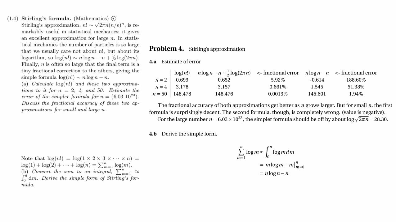
Problem 4. Stirling’s approximation

4.a Estimate of error

log(n!) n logn °n + 12 log(2ºn) <- fractional error n logn °n <- fractional error

n = 2 0.693 0.652 5.92% -0.614 188.60%n = 4 3.178 3.157 0.661% 1.545 51.38%

n = 50 148.478 148.476 0.0013% 145.601 1.94%

The fractional accuracy of both approximations get better as n grows larger. But for small n, the firstformula is surprisingly decent. The second formula, though, is completely wrong. (value is negative).

For the large number n = 6.03£1023, the simpler formula should be off by about logp

2ºn = 28.30.

4.b Derive the simple form.

nX

m=1logm º

Zn

0logmdm

= m logm °mØØnm=0

= n logn °n

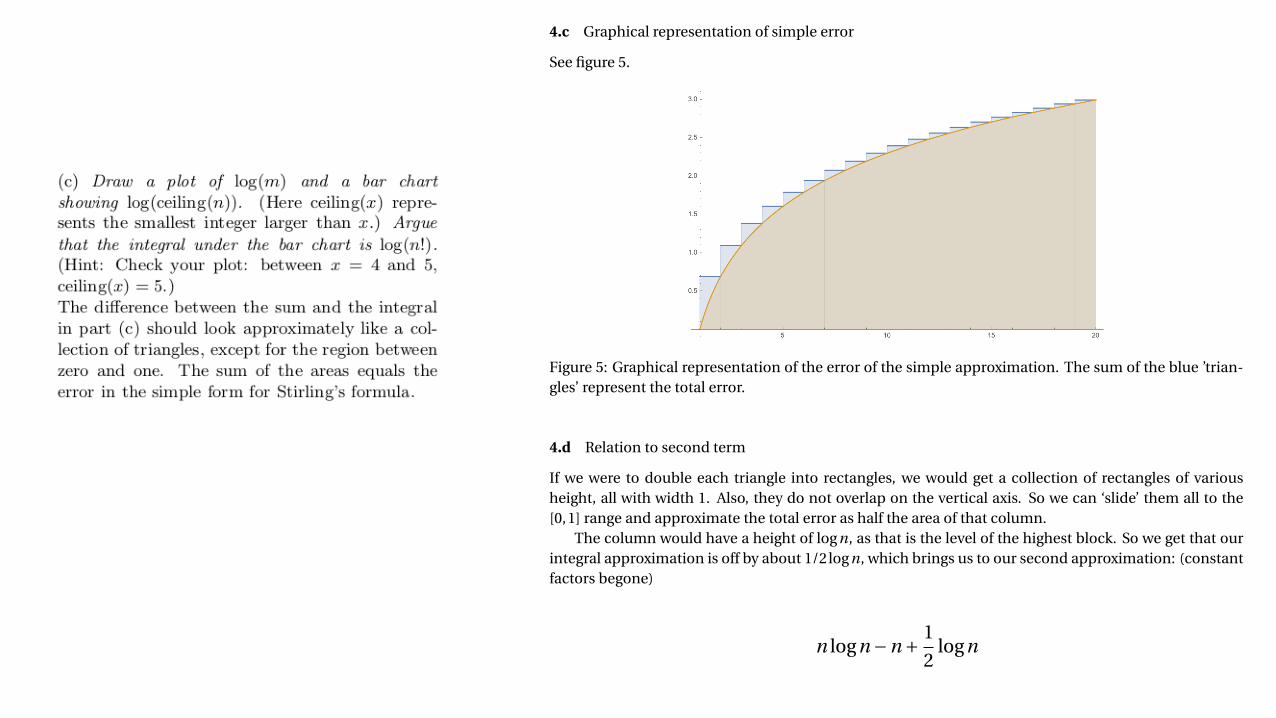
4.c Graphical representation of simple error

See figure 5.

Figure 5: Graphical representation of the error of the simple approximation. The sum of the blue ’trian-gles’ represent the total error.

4.d Relation to second term

If we were to double each triangle into rectangles, we would get a collection of rectangles of variousheight, all with width 1. Also, they do not overlap on the vertical axis. So we can ‘slide’ them all to the[0,1] range and approximate the total error as half the area of that column.

The column would have a height of logn, as that is the level of the highest block. So we get that ourintegral approximation is off by about 1/2logn, which brings us to our second approximation: (constantfactors begone)

8

Problem 4. Stirling’s approximation

4.a Estimate of error

log(n!) n logn °n + 12 log(2ºn) <- fractional error n logn °n <- fractional error

n = 2 0.693 0.652 5.92% -0.614 188.60%n = 4 3.178 3.157 0.661% 1.545 51.38%

n = 50 148.478 148.476 0.0013% 145.601 1.94%

The fractional accuracy of both approximations get better as n grows larger. But for small n, the firstformula is surprisingly decent. The second formula, though, is completely wrong. (value is negative).

For the large number n = 6.03£1023, the simpler formula should be off by about logp

2ºn = 28.30.

4.b Derive the simple form.

nX

m=1logm º

Zn

0logmdm

= m logm °mØØnm=0

= n logn °n

4.c Graphical representation of simple error

See figure 5.

Figure 5: Graphical representation of the error of the simple approximation. The sum of the blue ’trian-gles’ represent the total error.

4.d Relation to second term

If we were to double each triangle into rectangles, we would get a collection of rectangles of variousheight, all with width 1. Also, they do not overlap on the vertical axis. So we can ‘slide’ them all to the[0,1] range and approximate the total error as half the area of that column.

The column would have a height of logn, as that is the level of the highest block. So we get that ourintegral approximation is off by about 1/2logn, which brings us to our second approximation: (constantfactors begone)

8

n logn °n + 12

logn

9

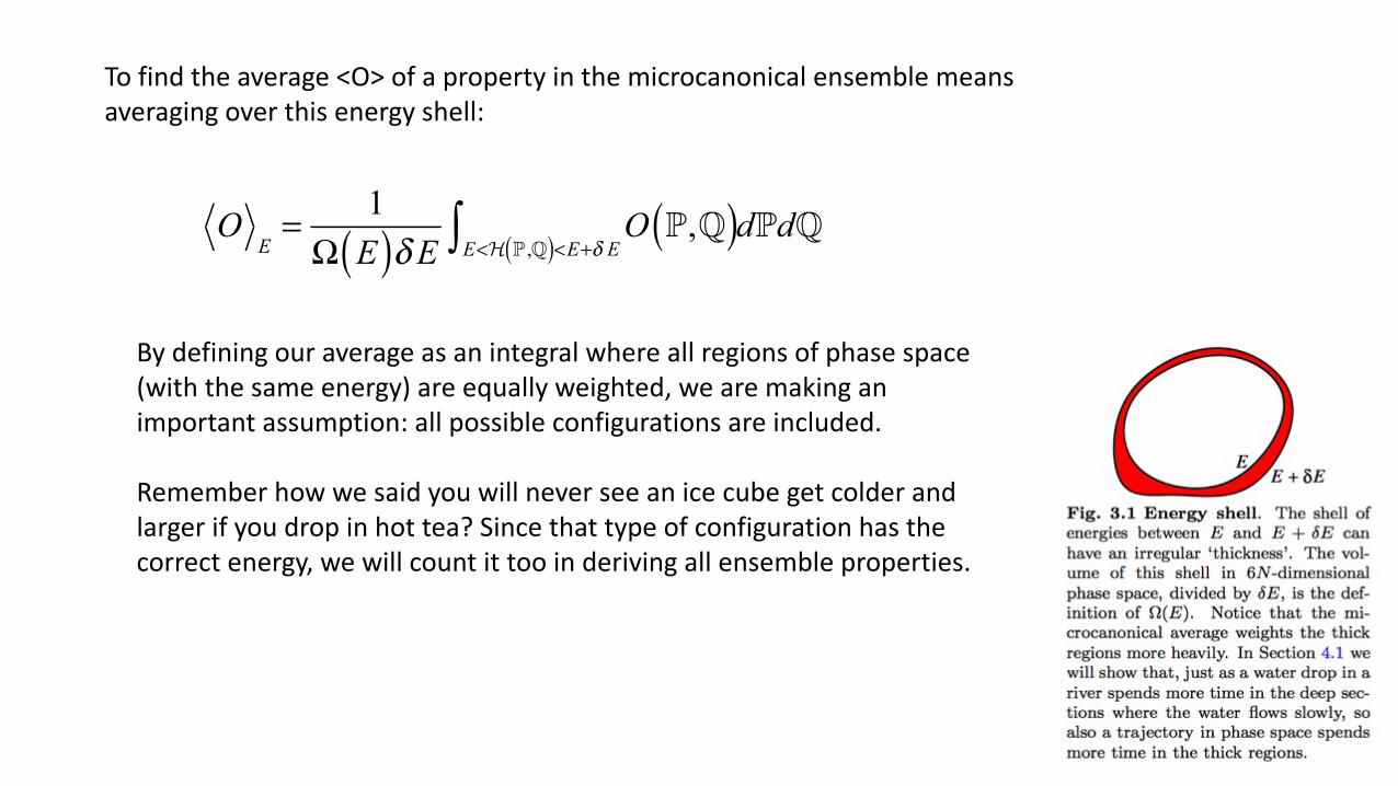
To find the average <O> of a property in the microcanonical ensemble means averaging over this energy shell:

OE= 1Ω E( )δ E O P,!( )

E<H P ,!( )<E+δ E∫ dPd!

By defining our average as an integral where all regions of phase space (with the same energy) are equally weighted, we are making an important assumption: all possible configurations are included.

Remember how we said you will never see an ice cube get colder and larger if you drop in hot tea? Since that type of configuration has the correct energy, we will count it too in deriving all ensemble properties.

( )( ) ( )

2 22 2 !2

! !2 NN

mPN N

N m N m N m-- æ ö

=ç ÷ +=

+ -è ø

n!∼ ne( )n 2πn ∼ n

e( )n

Configuration Space

We consider a monatomic ideal gas. The total energy is fixed = microcanonical ensemble. Consider only the set of positions; ignore the momenta.

There are 2N atoms. In a box of volume V= L3, what is the probability that the right half has N+m of the atoms, with N-m in the left half?

How many ways can 2N particles be distributed between the two halves? 22N. Then how many ways can N+m be on the right side? Use our standard combinatoric function:

We will use Stirling’s formula to evaluate these factorials:

Pm ≈= 2−2N

2Ne

⎛⎝⎜

⎞⎠⎟

2N

N +me

⎛⎝⎜

⎞⎠⎟

N+mN −me

⎛⎝⎜

⎞⎠⎟

N−m

=N2N N +m( )− N+m( ) N −m( )− N−m( )

= 1+mN( )− N+m( ) 1−mN( )− N−m( )

= 1+mN( ) 1−mN( )( )−N 1+mN( )−m 1−mN( )m

= 1−m2

N 2( )−N 1+mN( )−m 1−mN( )m

Ignore the normalizing prefactor for now, and expand:

At the last line, the next step is our frequent approximation:

1+ ε ≈ exp(ε )

(We assume m<<N.)

Pm ≈ e−m2

N 2⎛⎝⎜

⎞⎠⎟

−N

emN⎛

⎝⎞⎠

−m

e−m

N⎛⎝

⎞⎠

m

≈ P0 exp −m2N( )

21 expmmP

N Npæ ö

» -ç ÷è ø

Voila!

Now recognize that this is a Gaussian function. We set its integral equal to unity, since it is a probability, which allows us to fix the prefactor. The sets the standard deviation to:

σ = N2

QUESTION: Is it possible for this standard deviation to depend on the speed of the particles, that is, the temperature?

We will see that the properties of configuration space can be separated from the momentum space properties IF the energy does not depend on position, i.e., there is no potential energy for the Hamiltonian.

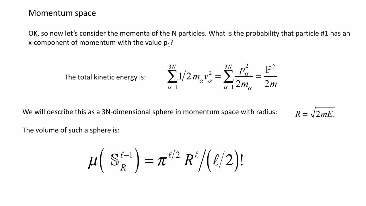
Momentum space

1 2mαα=1

3N

∑ vα2 =

pα2

2mαα=1

3N

∑ = P2

2m

µ SRℓ−1( ) = π ℓ 2 Rℓ ℓ 2( )!

OK, so now let’s consider the momenta of the N particles. What is the probability that particle #1 has an x-component of momentum with the value p1?

The total kinetic energy is:

We will describe this as a 3N-dimensional sphere in momentum space with radius:

The volume of such a sphere is:

R = 2mE.

Copyright Oxford University Press 2006 v2.0 --

56 Temperature and equilibrium

Fig. 3.2 The energy surface in mo-mentum space is the 3N−1 sphere ofradius R =

√2mE. The conditions

that the x-component of the momen-tum of atom #1 is p1 restricts us toa circle (or rather a 3N−2 sphere) ofradius R′ =

√2mE − p12. The con-

dition that the energy is in the shell(E,E + δE) leaves us with the annu-lar region shown in the inset.

The volume of the thin shell23 between E and E + δE is given by23Why is this not the surface area? Be-cause its width is an infinitesimal en-ergy δE, and not an infinitesimal thick-ness δR ≈ δE(∂R/∂E) = δE(R/2E).The distinction does not matter forthe ideal gas (both would give uniformprobability densities over all directionsof P) but it is important for interact-ing systems (where the thickness of theenergy shell varies, see Fig. 3.1).

shell volume

δE=

µ

(S3N−1√

2m(E+δE)

)− µ

(S3N−1√

2mE

)

δE

= dµ(S3N−1√

2mE

)/dE

=d

dE

(π3N/2(2mE)3N/2

/(3N/2)!

)

= π3N/2(3Nm)(2mE)3N/2−1/(3N/2)!

= (3Nm)π3N/2R3N−2/(3N/2)!. (3.14)

Given our microcanonical ensemble that equally weights all states withenergy E, the probability density for having any particular set of particlemomenta P is the inverse of this shell volume.Let us do a tangible calculation with this microcanonical ensemble.

Let us calculate the probability density ρ(p1) that the x-component ofthe momentum of the first atom is p1.24 The probability density that24It is a sloppy physics convention to

use ρ to denote probability densities ofall sorts. Earlier, we used it to denoteprobability density in 3N-dimensionalconfiguration space; here we use it todenote probability density in one vari-able. The argument of the function ρtells us which function we are consider-ing.

this momentum is p1 and the energy is in the range (E,E + δE) isproportional to the area of the annular region in Fig. 3.2. The spherehas radius R =

√2mE, so by the Pythagorean theorem, the circle has

radius R′ =√2mE − p12. The volume in momentum space of the

annulus is given by the difference in areas inside the two ‘circles’ (3N−2spheres) with momentum p1 and energies E and E + δE. We can useeqn 3.13 with $ = 3N − 1:

annular area

δE= dµ

(S3N−2√

2mE−p12

)/dE

=d

dE

(π(3N−1)/2(2mE − p1

2)(3N−1)/2/[(3N − 1)/2]!

)

= π(3N−1)/2(3N−1)m(2mE−p21)(3N−3)/2

/[(3N − 1)/2]!.

= (3N − 1)mπ(3N−1)/2R′3N−3/[(3N − 1)/2]! (3.15)

shell volumeδ E

=µ S

2m(E+δ E3N−1( )− µ S

2m(E )3N−1( )

δ E

=dµ S2m(E )

3N−1( ) dE

=ddE

π 3N 2 2mE( )3N 23N 2( )!( )

=π 3N 2 3Nm( ) 2mE( )3N 2−13N 2( )!

= 3Nm( )π 3N /2 R3N−2 3N 2( )!

We can evaluate the volume of the thin shell that contains all configurations with energy between E and E+DE:

annular areaδ E

= dµ S2mE− p1

2

3N−2⎛⎝⎜

⎞⎠⎟ dE

= ddE

π 3N−1( ) 2 2mE − p12( ) 3N−1( ) 2

3N −1( ) 2⎡⎣ ⎤⎦!⎛⎝

⎞⎠

=π 3N−1( ) 2 3N −1( )m 2mE − p12( ) 3N−3 2( )

3N −1( ) 2⎡⎣ ⎤⎦!

= 3N −1( )mπ 3N−1( ) 2 ′R 3N−3 3N −1( ) 2⎡⎣ ⎤⎦!









shell volume

δE=

µ

(S3N−1√

2m(E+δE)

)− µ

(S3N−1√

2mE

)

δE

= dµ(S3N−1√

2mE

)/dE

=d

dE

(π3N/2(2mE)3N/2

/(3N/2)!

)

= π3N/2(3Nm)(2mE)3N/2−1/(3N/2)!

= (3Nm)π3N/2R3N−2/(3N/2)!. (3.14)








annular area

δE= dµ

(S3N−2√

2mE−p12

)/dE

=d

dE

(π(3N−1)/2(2mE − p1

2)(3N−1)/2/[(3N − 1)/2]!

)

= π(3N−1)/2(3N−1)m(2mE−p21)(3N−3)/2

/[(3N − 1)/2]!.

= (3N − 1)mπ(3N−1)/2R′3N−3/[(3N − 1)/2]! (3.15)

But now we want to know how many of these configurations have a momentum p1 first particle. Look at the figure. Selecting out one component in the momentum-space sphere looks like a plane at a fixed height above the central plane, which intersects the shell with an annular region between two “circles.” We calculate this area:

( )( ) ( ) ( )

( )( )( )

( )( )

1

3 1 2 3 3

3 2 3 2

32 3

3 22 3 21

area volume

3 1 3 1 2 ! =

3 3 2 !

= 1 2

N N

N N

N

N

p annular shell

N m R NNm R N

R R R R

R R p mE

r

pp

- -

-

=

¢- -é ùë û

¢ ¢µ

¢ -

Now, take the ratio of this annular area to the volume of the shell, to get the probability of having the value p1:









shell volume

δE=

µ

(S3N−1√

2m(E+δE)

)− µ

(S3N−1√

2mE

)

δE

= dµ(S3N−1√

2mE

)/dE

=d

dE

(π3N/2(2mE)3N/2

/(3N/2)!

)

= π3N/2(3Nm)(2mE)3N/2−1/(3N/2)!

= (3Nm)π3N/2R3N−2/(3N/2)!. (3.14)








annular area

δE= dµ

(S3N−2√

2mE−p12

)/dE

=d

dE

(π(3N−1)/2(2mE − p1

2)(3N−1)/2/[(3N − 1)/2]!

)

= π(3N−1)/2(3N−1)m(2mE−p21)(3N−3)/2

/[(3N − 1)/2]!.

= (3N − 1)mπ(3N−1)/2R′3N−3/[(3N − 1)/2]! (3.15)

NOTE: That last term is less than or equal to unity, AND it is raised to a very high power. How does that not become zero?

REMINDER: E is the total energy of the N particles, and p1 is a momentum component of a single particle.

Let’s stare at this result a little while:









shell volume

δE=

µ

(S3N−1√

2m(E+δE)

)− µ

(S3N−1√

2mE

)

δE

= dµ(S3N−1√

2mE

)/dE

=d

dE

(π3N/2(2mE)3N/2

/(3N/2)!

)

= π3N/2(3Nm)(2mE)3N/2−1/(3N/2)!

= (3Nm)π3N/2R3N−2/(3N/2)!. (3.14)








annular area

δE= dµ

(S3N−2√

2mE−p12

)/dE

=d

dE

(π(3N−1)/2(2mE − p1

2)(3N−1)/2/[(3N − 1)/2]!

)

= π(3N−1)/2(3N−1)m(2mE−p21)(3N−3)/2

/[(3N − 1)/2]!.

= (3N − 1)mπ(3N−1)/2R′3N−3/[(3N − 1)/2]! (3.15)

How can the last term NOT be zero, since it is something less than 1 raised to a power of roughly Avogadro’s number?

The only way is if the argument is extremely close to unity.

This would then force R’ to be basically equal to R, so all of the useful ”surface area” must be right at the equator (for large N).

( )21

11 3exp

2 22p Npm EmE

ræ ö-

µ ç ÷è ø

( )( )

21

11 3exp

2 22 2 3p Npm Em E N

rp

æ ö-= ç ÷

è ø









shell volume

δE=

µ

(S3N−1√

2m(E+δE)

)− µ

(S3N−1√

2mE

)

δE

= dµ(S3N−1√

2mE

)/dE

=d

dE

(π3N/2(2mE)3N/2

/(3N/2)!

)

= π3N/2(3Nm)(2mE)3N/2−1/(3N/2)!

= (3Nm)π3N/2R3N−2/(3N/2)!. (3.14)








annular area

δE= dµ

(S3N−2√

2mE−p12

)/dE

=d

dE

(π(3N−1)/2(2mE − p1

2)(3N−1)/2/[(3N − 1)/2]!

)

= π(3N−1)/2(3N−1)m(2mE−p21)(3N−3)/2

/[(3N − 1)/2]!.

= (3N − 1)mπ(3N−1)/2R′3N−3/[(3N − 1)/2]! (3.15)

Hence, we can write....

1− p12

2mE = 1− ε ≈ exp(−ε ) = exp(− p12

2mE)

Again, since this is a Gaussian:

This is a very powerful result!

QUESTION: Is this an example of the Central Limit Theorem?

QUESTION: What does this say about an ice cube getting colder in hot tea? (Compare 𝛿𝑝 ≈2𝑚𝐸/3𝑁 to maximum latitude 2𝑚𝐸.)

QUESTION: Where is this function a maximum?

( )21

11 exp

22 BB

ppmk Tmk T

rp

æ ö= -ç ÷

è ø

( )( )

21

11 3exp

2 22 2 3p Npm Em E N

rp

æ ö-= ç ÷

è ø

Shortly we will have a good definition of temperature for the ideal gas, which will then give us the Boltzmann distribution:

A powerful derivation of the momentum probability distribution function for the ideal gas (microcanonical ensemble).

Here we take advantage of the relation kT=2E/3N, to be derived soon for the ideal gas.

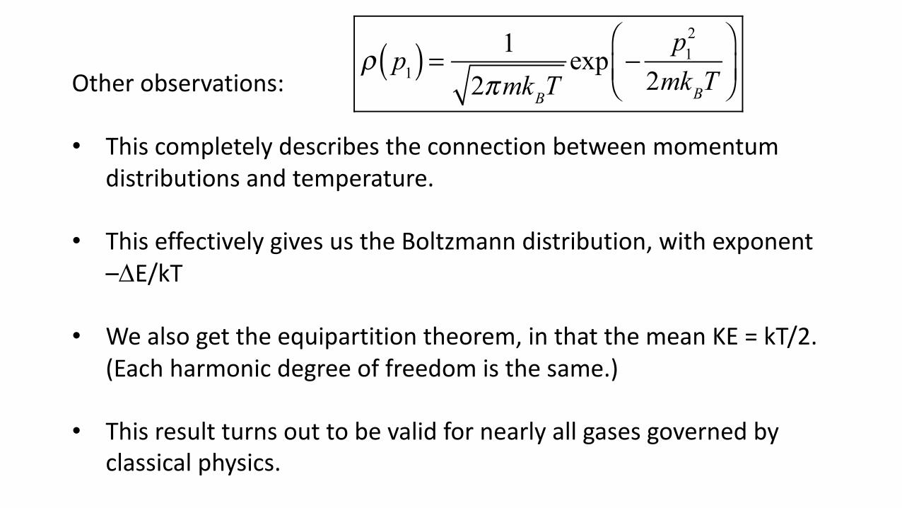
Other observations:

• This completely describes the connection between momentum distributions and temperature.

• This effectively gives us the Boltzmann distribution, with exponent –DE/kT

• We also get the equipartition theorem, in that the mean KE = kT/2. (Each harmonic degree of freedom is the same.)

• This result turns out to be valid for nearly all gases governed by classical physics.

ρ p1( ) = 1

2πmkBTexp −

p12

2mkBT⎛

⎝⎜⎞

⎠⎟

Documents

Lecture 9 PHYS 416