Lecture 9Chapter 22. Tests for two-way tables

Objectives

The chi-square test for two-way tables

(Award: NHST Test for Independence)

Two-way tables

Hypotheses for the chi-square test for two-way tables

Expected counts in a two-way table

Conditions for the chi-square test

Chi-square test for two-way tables of fit

Simpson’s paradox

400 1380416 1823188 1168

An experiment has a two-way factorial design if two categorical

factors are studied with several levels of each factor.

Two-way tables organize data about two categorical variables with any

number of levels/treatments obtained from a factorial design design or

two-way observational study.

Two-way tables

First factor: Parent smoking status

Second factor: Student smoking status

High school students were asked whether they smoke, and whether their

parents smoke:

Marginal distribution

The marginal distributions (in the “margins” of the table) summarize

each factor independently.

400 1380416 1823188 1168

Marginal distribution for parental smoking:

P(both parent)

= 1780/5375 = 33.1%

P(one parent) = 41.7%

P(neither parent) = 25.2%

The cells of the two-way table represent the intersection of a given level

of one factor with a given level of the other factor. They represent the

conditional distributions.

Conditional distribution of student smoking for different parental smoking statuses:

P(student smokes | both parent) = 400/1780 = 22.5%

P(student smokes | one parent) = 416/2239 =18.6%

P(student smokes | neither parent) = 188/1356 = 13.9%

400 1380416 1823188 1168

Conditional distribution

Hypotheses

A two-way table has r rows and c columns. H0 states that there is no

association between the row and column variables in the table.

Statistical Hypotheses

H0 : There is no association between the row and column variables

Ha : There is an association/relationship between the 2 variables

We will compare actual counts from the sample data with the counts

we would expect if the null hypothesis of no relationship were true.

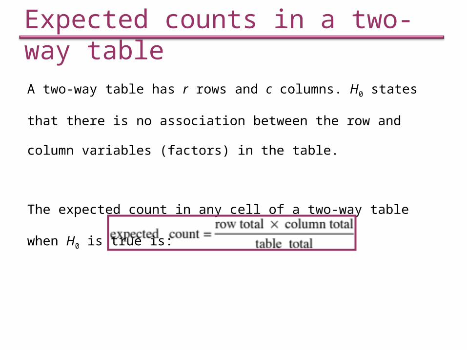
Expected counts in a two-way tableA two-way table has r rows and c columns. H0 states that there is no

association between the row and column variables (factors) in the

table.

The expected count in any cell of a two-way table when H0 is true is:

The expected count is the average count you would get for that cell if

the null hypotheses was true.

Cocaine addiction

Cocaine produces short-term feelings of physical and

mental well being. To maintain the effect, the drug

may have to be taken more frequently and at higher

doses. After stopping use, users will feel tired, sleepy

and depressed. 

A study compares the rates of successful rehabilitation for cocaine addicts

following 1 of 3 treatment options:

1: antidepressant treatment (desipramine)

2: standard treatment (lithium)

3: placebo (“sugar pill”)

Cocaine addiction

Calculate the expected cell counts if relapse is independent of the treatment.

25*26/74 ≈ 8.7825*0.35

16.2225*0.65

9.1426*0.35

16.8625*0.65

8.0823*0.35

14.9225*0.65

Desipramine

Lithium

Placebo

35% 35%35%

Expected %

Observed %

Expected relapse counts

No Yes

Situations appropriate for the chi-square test

The chi-square test for two-way tables looks for evidence of association

between multiple categorical variables (factors) in sample data. The

samples can be drawn either:

By randomly selecting SRSs from different populations (or from a

population subjected to different treatments)

girls vaccinated for HPV or not, among 8th graders and 12th graders

remission or no remission for different treatments

Or by taking 1 SRS and classifying the individuals according to 2

categorical variables (factors)

11th graders’ smoking status and parents’ status

When looking for associations between two categorical/nominal variables.

We can safely use the chi-square test when:

no more than 20% of expected counts are less than 5 (< 5)

all individual expected counts are 1 or more (≥1)

What goes wrong? With small expected cell counts the sampling

distribution will not be chi-square distributed.

Statistician’s note: If one factor has many levels and too many expected counts

are too low, you might be able to “collapse” some of the levels (regroup them)

and thus have large-enough expected counts.

P-value: P(2 variable ≥ calculated 2 | H0 is true)

The 2 statistic sums over all r x c cells in the table

When H0 is true, the 2 statistic

follows ~ 2 distribution with

(r-1)(c-1) degrees of freedom.

count expected

count expected -count observed

22

The chi-square test for two-way tablesH0 : there is no association between the row and column variables

Ha : H0 is not true

pdf 0.25 0.2 0.15 0.1 0.05 0.025 0.02 0.01 0.005 0.0025 0.001 0.00051 1.32 1.64 2.07 2.71 3.84 5.02 5.41 6.63 7.88 9.14 10.83 12.12 2 2.77 3.22 3.79 4.61 5.99 7.38 7.82 9.21 10.60 11.98 13.82 15.20 3 4.11 4.64 5.32 6.25 7.81 9.35 9.84 11.34 12.84 14.32 16.27 17.73 4 5.39 5.99 6.74 7.78 9.49 11.14 11.67 13.28 14.86 16.42 18.47 20.00 5 6.63 7.29 8.12 9.24 11.07 12.83 13.39 15.09 16.75 18.39 20.51 22.11 6 7.84 8.56 9.45 10.64 12.59 14.45 15.03 16.81 18.55 20.25 22.46 24.10 7 9.04 9.80 10.75 12.02 14.07 16.01 16.62 18.48 20.28 22.04 24.32 26.02 8 10.22 11.03 12.03 13.36 15.51 17.53 18.17 20.09 21.95 23.77 26.12 27.87 9 11.39 12.24 13.29 14.68 16.92 19.02 19.68 21.67 23.59 25.46 27.88 29.67 10 12.55 13.44 14.53 15.99 18.31 20.48 21.16 23.21 25.19 27.11 29.59 31.42 11 13.70 14.63 15.77 17.28 19.68 21.92 22.62 24.72 26.76 28.73 31.26 33.14 12 14.85 15.81 16.99 18.55 21.03 23.34 24.05 26.22 28.30 30.32 32.91 34.82 13 15.98 16.98 18.20 19.81 22.36 24.74 25.47 27.69 29.82 31.88 34.53 36.48 14 17.12 18.15 19.41 21.06 23.68 26.12 26.87 29.14 31.32 33.43 36.12 38.11 15 18.25 19.31 20.60 22.31 25.00 27.49 28.26 30.58 32.80 34.95 37.70 39.72 16 19.37 20.47 21.79 23.54 26.30 28.85 29.63 32.00 34.27 36.46 39.25 41.31 17 20.49 21.61 22.98 24.77 27.59 30.19 31.00 33.41 35.72 37.95 40.79 42.88 18 21.60 22.76 24.16 25.99 28.87 31.53 32.35 34.81 37.16 39.42 42.31 44.43 19 22.72 23.90 25.33 27.20 30.14 32.85 33.69 36.19 38.58 40.88 43.82 45.97 20 23.83 25.04 26.50 28.41 31.41 34.17 35.02 37.57 40.00 42.34 45.31 47.50 21 24.93 26.17 27.66 29.62 32.67 35.48 36.34 38.93 41.40 43.78 46.80 49.01 22 26.04 27.30 28.82 30.81 33.92 36.78 37.66 40.29 42.80 45.20 48.27 50.51 23 27.14 28.43 29.98 32.01 35.17 38.08 38.97 41.64 44.18 46.62 49.73 52.00 24 28.24 29.55 31.13 33.20 36.42 39.36 40.27 42.98 45.56 48.03 51.18 53.48 25 29.34 30.68 32.28 34.38 37.65 40.65 41.57 44.31 46.93 49.44 52.62 54.95 26 30.43 31.79 33.43 35.56 38.89 41.92 42.86 45.64 48.29 50.83 54.05 56.41 27 31.53 32.91 34.57 36.74 40.11 43.19 44.14 46.96 49.64 52.22 55.48 57.86 28 32.62 34.03 35.71 37.92 41.34 44.46 45.42 48.28 50.99 53.59 56.89 59.30 29 33.71 35.14 36.85 39.09 42.56 45.72 46.69 49.59 52.34 54.97 58.30 60.73 30 34.80 36.25 37.99 40.26 43.77 46.98 47.96 50.89 53.67 56.33 59.70 62.16 40 45.62 47.27 49.24 51.81 55.76 59.34 60.44 63.69 66.77 69.70 73.40 76.09 50 56.33 58.16 60.35 63.17 67.50 71.42 72.61 76.15 79.49 82.66 86.66 89.56 60 66.98 68.97 71.34 74.40 79.08 83.30 84.58 88.38 91.95 95.34 99.61 102.70 80 88.13 90.41 93.11 96.58 101.90 106.60 108.10 112.30 116.30 120.10 124.80 128.30 100 109.10 111.70 114.70 118.50 124.30 129.60 131.10 135.80 140.20 144.30 149.40 153.20

Table A

Ex: df = 6

If 2 = 15.9

the P-value

is between

0.01 −0.02.

74.1092.14

92.1419

08.8

08.84

86.16

86.1619

14.9

14.97

22.16

22.1610

78.8

78.815

22

22

222

158.78

1016.22

79.14

1916.86

48.08

1914.92

Desipramine

Lithium

Placebo

No relapse RelapseTable of counts:

“actual/expected,” with

three rows and two

columns:

df = (3 − 1)(2 − 1) = 2

We compute the X2 statistic:

Using Table D: 10.60 < X2 < 11.98 0.005 > P > 0.0025

The P-value is very small (JMP gives P = 0.0047) and we reject H0.

There is a significant relationship between treatment type (desipramine, lithium,

placebo) and outcome (relapse or not).

Interpreting the 2 output

When the 2 test is statistically significant:

The largest components indicate which condition(s) are most different

from H0. You can also compare the observed and expected counts, or

compare the computed proportions in a graph.

The largest X2 component, 4.41, is for

desipramine/norelapse. Desipramine has

the highest success rate (see graph).

4.41 2.39 0.50 0.27 2.06 1.12

2 components

DesipramineLithiumPlacebo

No relapse Relapse

Influence of parental smoking

Here is a computer output for a chi-square test performed on the data from

a random sample of high school students (rows are parental smoking

habits, columns are the students’ smoking habits). What does it tell you?

Is the sample size sufficient?

What are the hypotheses?

Are the data ok for a 2 test?

What else should you ask?

What is your interpretation?

Caution with categorical data

An association that holds for all of several groups can reverse direction

when the data are combined to form a single group. This reversal is

called Simpson's paradox.

Kidney stones

It turns out that for any given patient that PCNL is more likely to result in failure. Can you think of a reason why?

A study compared the success rates of

two different procedures for removing

kidney stones: open surgery and

percutaneous nephrolithotomy (PCNL),

a minimally invasive technique.

Open surgery PCNL Open surgery PCNLSuccess 81 234 Success 192 55Failure 6 36 Failure 71 25% failure 7% 13% % failure 27% 31%

Small stones

273 289 77 61

22% 17%

Open surgery PCNL Open surgery PCNLSuccess 81 234 Success 192 55Failure 6 36 Failure 71 25% failure 7% 13% % failure 27% 31%

Small stones Large stones

The procedures are not chosen randomly by surgeons! In fact, the minimally

invasive procedure is most likely used for smaller stones (with a good chance of

success) whereas open surgery is likely used for more problematic conditions.

Open surgery PCNL Open surgery PCNLSuccess 81 234 Success 192 55Failure 6 36 Failure 71 25% failure 7% 13% % failure 27% 31%

Small stones

273 289 77 61

22% 17%

For both small stones and large stones, open surgery has a lower failure rate.

This is Simpson’s paradox. The more challenging cases with large stones tend

to be treated more often with open surgery, making it appear as if

the procedure were less reliable overall.

Beware of lurking variables!