Massachusetts Institute of Technology 6.763 2003 Lecture 8

Lecture 8: Perfect DiamagnetismOutline

1. Description of a Perfect Diamagnet• Method I and Method II• Examples

2. Energy and Coenergy in Methods I and II

3. Levitating magnets and Maglev trains

September 30, 2003

Massachusetts Institute of Technology 6.763 2003 Lecture 8

Description of Perfect Diamagetism

Surface currents or internal induced magnetization?

Massachusetts Institute of Technology 6.763 2003 Lecture 8

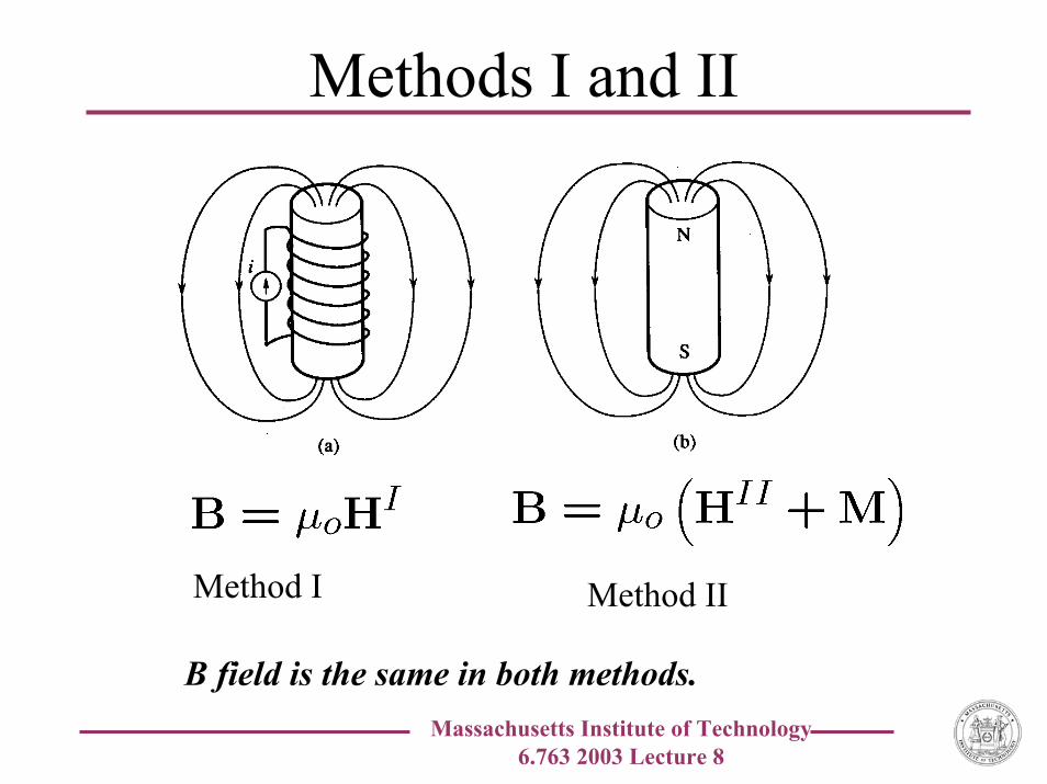
Methods I and II

Method I Method II

B field is the same in both methods.

Massachusetts Institute of Technology 6.763 2003 Lecture 8

Example: Magnetized Sphere

For this example: Laplace’s equation

Massachusetts Institute of Technology 6.763 2003 Lecture 8

Boundary ConditionsInside the sphere:

Outside the sphere:

Boundary Conditions:

Therefore,

Massachusetts Institute of Technology 6.763 2003 Lecture 8

Magnetized Sphere

Massachusetts Institute of Technology 6.763 2003 Lecture 8

Magnetized Sphere in field

For this to describe a superconductor (bulk limit), then B=0 inside.

Therefore,

So that

Massachusetts Institute of Technology 6.763 2003 Lecture 8

Comparison of MethodsMethod I Method II

Inside a bulk superconducting sphere:

B field is the same, but not H.

Massachusetts Institute of Technology 6.763 2003 Lecture 8

Methods I and II: SummaryMethod I Method II

Maxwell’s Equations

London Equations

Massachusetts Institute of Technology 6.763 2003 Lecture 8

Why Method IIQuestion: The constitutive relations and London’s Equations have gotten much more difficult. So why do Method II?

Answer: The Energy and Thermodynamics are easier, especially when there is no applied current.

So we will find the energy stored in both methods.

Poynting’s theorem is a result of Maxwell’s equation, so both methods give

Massachusetts Institute of Technology 6.763 2003 Lecture 8

Method I: The EnergyCombining the constitutive relations with Poynting’s theorem,

Power dW/dt in the E&M field

The energy stored in the electromagnetic field is

So that the energy W is a function of D, B, and ΛJsI= vs .

However, one rarely has control over these variables, but rather over their conjugates E, HI, and Js

I.

Massachusetts Institute of Technology 6.763 2003 Lecture 8

Method I: The CoenergyThe coenergy is a function of E, HI, and Js

I is defined by

and with

givesMQSEQS

(The coenergy is the Free Energy at zero temperature.)

Massachusetts Institute of Technology 6.763 2003 Lecture 8

Interpretation of the CoenergyConsider the case where there are only magnetic fields:

The energy and coenergy contain the same information.

Massachusetts Institute of Technology 6.763 2003 Lecture 8

Method II

In the important case when of the MQS limit and

Note that these two relations apply also in free space.

Massachusetts Institute of Technology 6.763 2003 Lecture 8

Example: Energy of a Superconducting Sphere

Massachusetts Institute of Technology 6.763 2003 Lecture 8

Magnetic Levitation

Massachusetts Institute of Technology 6.763 2003 Lecture 8

Magnetic vs. Gravitational Forces

η

Massachusetts Institute of Technology 6.763 2003 Lecture 8

Magnetic Levitation Equilibrium Point

Force mainly due to bending of flux lines here.

Force is upwards

Equilibrium point

Massachusetts Institute of Technology 6.763 2003 Lecture 8

Levitating magnets and trains

B = 1 TeslaArea = 0.5 cm2

η0 = 1 cmForce = 1 Newton

Enough to lift magnet, but not a train

B = 2 TeslaArea = 100 cm2

η0 = 10 cmForce = 1,200 Newtons

Enough to lift a train

Massachusetts Institute of Technology 6.763 2003 Lecture 8

Maglev Train

Magnets on the train are superconducting magnets; the rails are ohmic!

Massachusetts Institute of Technology 6.763 2003 Lecture 8

Principle of MaglevThe train travels at a velocity U, and the moving flux lines and the rails “see” a moving magnetic field at a frequency of

ω ~ U/R. If this frequency is much larger than the inverse of the magnetic diffusion time,

then the flux lines are “repelled” from the ohmic rails.

From the previous numbers, U > 40 km/hr for levitation.

Massachusetts Institute of Technology 6.763 2003 Lecture 8

Real trains have wheels and high-voltage rails

Synchronous motor action down the rails provides thrust to accelerate train to the needed velocity to levitate, and provides a source of energy to further accelerate the train and to overcome the losses due to drag from the wind.

Massachusetts Institute of Technology 6.763 2003 Lecture 8

Our Approach to SuperconductivitySuperconductor as a perfect conductor & perfect diamagnet

Macroscopic Quantum Model Ψ(r)

Supercurrent Equation Js(r)

Ginzburg-Landau

Ψ(r) = | Ψ(r)|2 e iθ(r,t)

BCS

Type II SuperconductivityLarge-Scale Applications

Josephson EquationsSmall-Scale Applications

Classica

l

Mac

rosc

opic Q

uant

um M

odel

Microscopic Quantum