Lecture 8 - Gauss’s LawA Puzzle...

Example

Calculate the potential energy, per ion, for an infinite 1D ionic crystal with separation a; that is, a row of equally

spaced charges of magnitude e and alternating sign.

Hint: The power-series expansion of Log[1 + x] may be of use.

Solution

Suppose the array is built inwards from the left (that is, from negative infinity) as far as a particular ion. To add

the next positive ion on the right, the amount of external work required equals

- k e2

a+ k e2

2 a- k e2

3 a+ · · · = - k e2

a1- 1

2 + 13 + · · · (1)

The terms in parenthesis look remarkably similar to the Taylor series of Log[1 + x] when x = 1. (What is the

Taylor series of Log[1 + x]? ⅆⅆx

Log[1 + x] = 11+x

= 1 - x + x2 - · · ·, and integrating both sides yields

Log[1 + x] = x - x2

2+ x3

3- · · ·, since the right hand side is a polynomial expansion, it is also the Taylor series of

Log[1 + x]. This Taylor series is converging for -1 < x ≤ 1 (with convergence on -1 < x < 1 assured by the

alternating series test)). Therefore the work required to bring this charge in equals - k e2

aLog[2], which equals the

energy of the infinite chain per ion.

The addition of further particles on the right doesn’t affect the energy involved in assembling the previous ones, so

this result is indeed the energy per ion in the entire infinite (in both directions) chain. The result is negative, which

means that it requires energy to move the ions away from each other. This makes sense, because the two nearest

neighbors are of opposite sign.

Note that this is an exact result! It does not assume that a is small. Getting such a nice closed form is much more

difficult in 2 and 3 dimensions. □

Theory

Visualizing the Electric Field (Extended)

Electric Field Lines

Advanced Section: Escaping Field Lines

Math Background: What is a Surface Integral?

We are already familiar with surface integrals of scalar functions. For example, the surface area of a sphere with

radius R centered at the origin is given by

∫surfaceⅆa = ∫0

2 π∫0πR2 Sin[θ] ⅆθ ⅆϕ = 4 π R2 (4)

Although we use spherical coordinates in this particular problem, we could also have used Cartesian coordinates

Printed by Wolfram Mathematica Student Edition

Although spherical particular problem,

(with ⅆa = ⅆx ⅆy) or any other coordinate system.

More generally, suppose we are given a function f [θ, ϕ] defined everywhere on the surface of the spherical shell

of radius R. What is the integral of f [θ, ϕ] across the entire spherical shell? This requires a very minor modifica-

tion to the formula above, namely,

∫surfacef [θ, ϕ] ⅆa = ∫0

2 π∫0πf [θ, ϕ] R2 Sin[θ] ⅆθ ⅆϕ (5)

We would need to know the specific function f [θ, ϕ] to explicitly evaluate this integral, but we observe that the

surface area is merely a specific case of Equation (5) with f [θ, ϕ] = 1 everywhere on the sphere.

Lastly, rather than being given a scalar function f [θ, ϕ], we could be given a vector function F[θ, ϕ] defined

everywhere on the sphere. In such a case, we define the surface integral to be

∫surfaceF[θ, ϕ] · ⅆa = ∫surface

F[θ, ϕ] · ⅆa ⅆa (6)

No need to panic! The right hand side is simply the same surface integral from Equation (5), except that now the

scalar function is the dot product of two vectors. The first vector F[θ, ϕ] is the function that you are integrating

over the sphere. The second vector ⅆa is a unit vector of an infinitesimal patch in the direction normal to the

surface. On the sphere, the unit normal vector at any point is given by ⅆa= r, so that we can write the surface

integral as

∫surfaceF[θ, ϕ] · ⅆa

ⅆa = ∫0

2 π∫0πF[θ, ϕ] · r R2 Sin[θ] ⅆθ ⅆϕ (7)

For closed surfaces, we take the unit normal to be pointing outwards by convention. For open surfaces, you can

arbitrarily choose between the two possible directions that the unit vector can point (if you switch, it will flip the

sign of the surface integral).

Usually, we will be working in setups where the unit normal vector is obvious. For example, if we have a sheet in

the x-y plane, then the unit normal vector will be z (or -z, you can choose either as long as you are consistent

throughout your surface integral) at all points. Similarly, if we have a cylinder whose axis lies on the z-axis, then

the unit normal vector at its top cap will be z (remembering that unit normal vectors point outwards for closed

surfaces) and -z at its bottom cap. Finally, in cylindrical coordinates (ρ, θ, z), the unit vector will be ρ for all

points along the curved surface of the cylinder.

Guass’s Law

An incredibly useful and beautiful result, Gauss’s Law is definitely worth memorizing! Here we write it for a

discrete and continuous charge distribution.

The integral ∫ E ·ⅆa over the surface, equals 1ϵ0

times the total charge enclosed by the surface,

∫ E · ⅆa = 1ϵ0∑j q j =

1ϵ0 ∫

ρ ⅆv (8)

For a combination of both (for example, a point charge near an infinite sheet), the Principle of Superposition tells

us that we sum over the discrete charges and integrate over the charge distributions within our surface.

Example

Find the electric field due to an infinite line of charge with uniform charge density λ.

2 Lecture 8 - 02-02-2017.nb

Printed by Wolfram Mathematica Student Edition

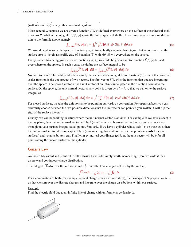
Solution

By symmetry, the electric field must point radially outwards from the line of charge.

Out[21]=

Cylinder

Show E

Show a

We can use a cylinder whose axis lies on the line of charge and calculate ∫ E ·ⅆa along this cylinder. Since E

points radially, E ·ⅆa = 0 along the (flat) top and bottom of the cylinder, and by radial symmetry, E ·ⅆa = E[r] ⅆa

will be a constant value everywhere along the cone (where E[r] is the magnitude of the electric field at a distance r

from the wire). Therefore, Gauss's Law yields

∫ E · ⅆa = E[r] ∫ ⅆa = E[r] (2 π r L) = λ L

ϵ0(9)

which yields

E[r] = λ

2 π r ϵ0(10)

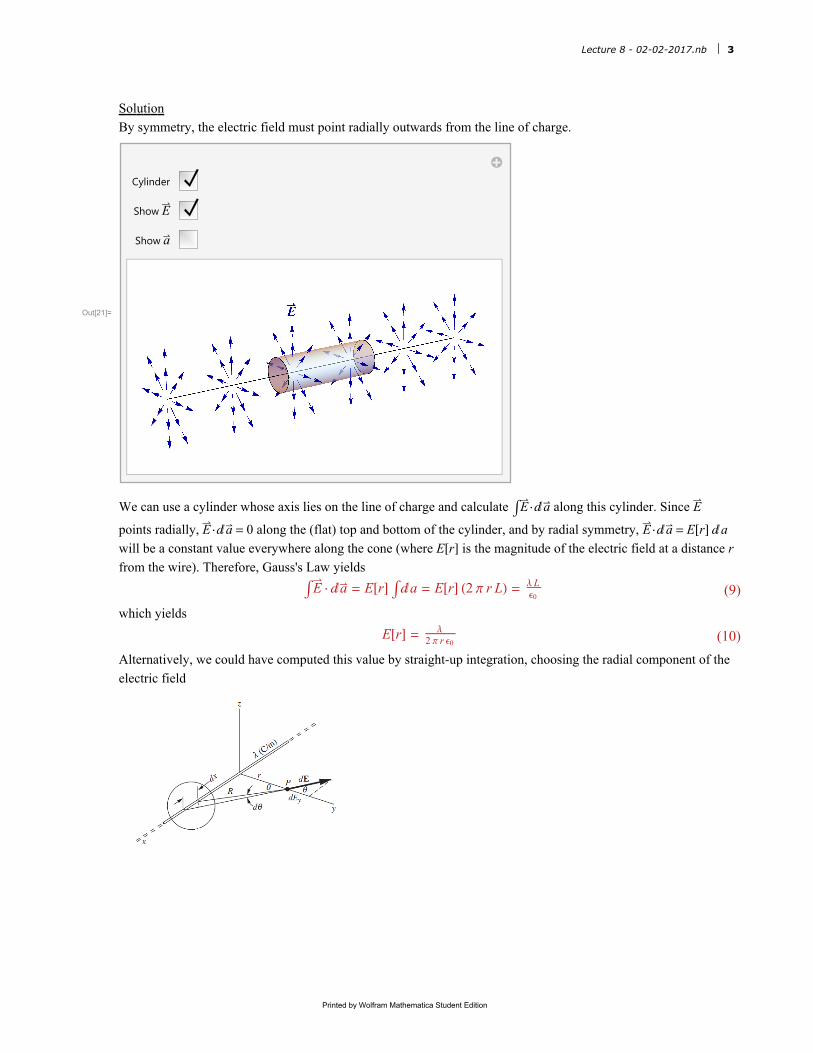
Alternatively, we could have computed this value by straight-up integration, choosing the radial component of the

electric field

Lecture 8 - 02-02-2017.nb 3

Printed by Wolfram Mathematica Student Edition

E[r] = ∫-∞∞ k λ ⅆx

x2+r2r

x2+r21/2

= k λ x

r x2+r21/2

x=-∞

x=∞

= 2 k λ

r

= λ

2 π r ϵ0

This yields the same result as above, but after significantly more work. □

A Note about Symmetry

The key to the last problem was proving that for a line of charge lying on the x-axis, the electric field E = E[r] r

points radially away from the wire. Let’s prove this explicitly.

If the infinitely long wire lies along the x-axis, then the points on the wire are given by (x, 0, 0) where

x ∈ (-∞, ∞). Let us consider the electric field at a point (0, 0, z), and let us call the electric field E = ⟨Ex, Ey, Ez⟩.

First, let us flip the setup along the x = 0 as shown below, which means that every point (and every vector) goes

from (x, y, z)→ (-x, y, z). Therefore the electric field will go from ⟨Ex, Ey, Ez⟩ → ⟨-Ex, Ey, Ez⟩, shown by the solid

arrow → dashed arrow. However, since every point (x, 0, 0) on the line of charge goes to another point (-x, 0, 0)

on the line of charge, and the point of interest (0, 0, z)→ (0, 0, z) does not change, the physical setup of the

problem remains exactly the same. Therefore, the electric field before and after the reflection must be the same,

and this is only possible if Ex = 0.

Similarly, consider a reflection about the y = 0 plane, so that every point goes from (x, y, z)→ (x, -y, z). Therefore

the electric field will go from ⟨0, Ey, Ez⟩ → ⟨0, -Ey, Ez⟩. Each point on the line of charge will not be changed

4 Lecture 8 - 02-02-2017.nb

Printed by Wolfram Mathematica Student Edition

(x, 0, 0)→ (x, 0, 0), and similarly the point of interest will not change (0, 0, z)→ (0, 0, z), so that once again the

physical setup is the same and hence the electric field must be the same. This can only happen in Ey = 0.

We conclude that at the point (0, 0, z), the electric field point straight up (i.e. radially away) from the line of

charge. We can generalize this result to find the direction of the electric field at an arbitrary point (x, y, z) using

symmetry. First, we note that because the wire is infinitely long, translating along the x-direction cannot change

the electric field, since we could equally well have defined our origin at some other point (X , 0, 0) and the physi-

cal setup would be identical to that found above, so that the electric field at (X , 0, z) must point in the z direction.

Finally, we use the rotational symmetry of the setup (i.e. rotating our coordinate system about the x-axis) to find

that the electric field at any point (x, y, z) points radially outward from the wire in the direction ⟨0, y, z⟩.

Problems

Field from a Cylindrical Shell

Example

Consider a charge distribution in the form of an infinitely long hollow circular cylinder (like a long charged pipe)

of radius R. If the cylinder has uniform charge per unit area σ, what is the electric field inside and outside the

cylinder?

Solution

The electric field inside the cylinder must be pointing radially about the axis of symmetry. Therefore, using a

Gaussian surface of a small cylinder with radius r < R and length l placed along the axis of the large cylinder, we

find that

E (2 π r l) = qin

ϵ0= 0 (12)

because there is no charge inside the cylindrical shell. Thus, E = 0 for all r < R.

The electric field outside the cylinder is found using a the same Gaussian surface but with r > R so that

E (2 π r l) = qin

ϵ0= 2 π R l σ

ϵ0(13)

or equivalently E = Rr

σϵ0

. Since the charge per unit length on the cylindrical shell equals 2 π R σ, E = (2 π R σ)2 π r ϵ0

so

that the electric field outside the cylinder is the same as if all of the charge was concentrated at on the axis of the

cylinder.

These results are very interesting, but let me point out one subtlety in this result. If you ask for the electric field

Lecture 8 - 02-02-2017.nb 5

Printed by Wolfram Mathematica Student Edition

very interesting, point subtlety you

E[r] as a function of the radial distance r from the cylindrical shell, then starting at ∞ and coming towards the axis

the answer will be

E[r] =R

r

σ

ϵ0r > R

0 r < R(14)

This implies that at r = R, there is a discontinuity; the value of E[r]→ σϵ0

from the outside of the cylindrical shell

and E[r]→ 0 from the inside of the shell. This begs the question, what exactly is the electric field at r = R? As we

will see from the electric field of an infinite plane, the answer will be E[R] = σ2 ϵ0

, and you are encouraged to do the

explicit calculation yourself! For now, we note that E[R] is the average of the values two limits of E[r] from inside

and outside the cylindrical shell. □

Extra Problem: Field from a Cylindrical Shell, Right and Wrong

Example

Find the electric field outside a uniformly charged hollow cylindrical shell with radius R and charge density σ, an

infinitesimal distance away from it. Do this in the following two ways:

1. Slice the shell into parallel infinite rods, and integrate the field contributions from all the rods. You should

obtain the incorrect result of σ2 ϵ0

.

2. Why isn't the result correct? Explain how to modify it to obtain the correct result of σϵ0

. Hint: You could very

well have performed the above integral in an effort to obtain the electric field an infinitesimal distance inside the

cylinder, where we know the field is zero. Does the above integration provide a good description of what's going

on for points on the shell that are very close to the point in question?

3. Confirm that the result equals σϵ0

by straight up integration assuming that the point is a finite distance z away

from the center of the cylinder. What happens when z < R, z = R, and z > R?

Solution

1. Let the rods be parameterized by the angle θ as shown in the diagram below.

The width of a rod is R ⅆθ, so its effective charge per unit length is λ =σ (R ⅆθ). The rod is a distance 2 R Sin θ2

from the point P in question, which is infinitesimally close to the top of the cylinder. Only the vertical component

of the field from the rod survives, and this brings in a factor of Sin θ2. Using the fact that the field from a rod is

λ2 π ϵ0 r

, we find that the field at the top of the cylinder is (incorrectly)

2 ∫0π σ R ⅆθ

2 π ϵ02 R Sin θ2 Sin θ2 =

σ

2 π ϵ0 ∫0πⅆθ = σ

2 ϵ0 (15)

Interestingly, we see that for a given angular width of a rod, all rods yield the same contribution to the vertical

electric field at P (since the ones further away from it contribute at a better angle).

6 Lecture 8 - 02-02-2017.nb

Printed by Wolfram Mathematica Student Edition

2. As stated in the problem, it is no surprise that this answer is incorrect, since the same calculation would suppos-

edly yield the field just inside the cylinder too, where it is zero instead of σϵ0

. However, this calculation does yield

the average of these two values.

The reason why the calculation is invalid is that it doesn’t correctly describe the field due to rods very close to the

given point, that is, for rods with θ ≈ 0. It is incorrect for two reasons. First, the distance from a rod to the given

point is not equal to 2 R Sin θ2. Additionally, the field does not point along the line from the rod to the top of the

cylinder. It points more vertically, so the extra factor of Sin θ2 which we used to pick out the vertical component

isn’t valid.

What is true is that if we remove a thin strip from θ = - ϕ2

to θ = ϕ2

(for very small ϕ≪ 1) at the top of the cylinder,

then the above integral is valid for the remaining part of the cylinder. In other words, the electric field due to the

remaining cylinder will be 2 π-ϕ2 π

σ2 ϵ0

≈ σ2 ϵ0

since we can make 2 π-ϕ2 π

arbitrarily close to 1. By superposition, the

total field of the entire cylinder in this field of σ2 ϵ0

plus the field due to the thin strip at the top. But if the point in

question is infinitesimally close to the cylinder, then the thin strip will look like an infinite plane, the field of

which we know is σ2 ϵ0

. The desired total field is then

Eoutside = Ecylinder minus strip + Estrip =σ

2 ϵ0+ σ

2 ϵ0= σ

ϵ0(16)

Einside = Ecylinder minus strip - Estrip =σ

2 ϵ0- σ

2 ϵ0= 0 (17)

where the minus sign in Einside comes from the fact that Estrip (like an infinite sheet) points in different directions

inside and outside the cylinder.

Technical note: We have two infinitesimally small quantities in this problem: the width ϕ of the strip that we are

removing from the cylinder and the infinitesimal distance of the point P from the cylinder. You may (or at least

should) be wondering which of these two infinitesimally small quantities is smaller. This is an important point to

keep track of - if you are blasé about the matter and simply send both quantities to 0 without regard, you could end

up with wrong results! In this problem, we want for the distance from P to the cylinder to be smaller, and indeed

that is the case. For we first picked a small ϕ (which we can make as small as we like) and then we considered a

point P which was essentially touching the cylinder but on the outside; you can think of this as once you fix ϕ, you

bring P in extremely close to the cylinder (and therefore extremely close to the thin strip).

3. Orient the cylinder’s axis to lie on the y-axis and consider the electric field at the point (0, 0, z).

Lecture 8 - 02-02-2017.nb 7

Printed by Wolfram Mathematica Student Edition

Define the distance from the wire at angle θ to the point (0, 0, z) to be r, which by the Law of Cosines equals

r2 = R2 + z2 - 2 R z Cos[θ]. Using the charge density λ =σ (R ⅆθ), the electric field λ2 π ϵ0 r

from an infinite wire,

and the z-component z-R Cos[θ]r

of the electric field,

E = ∫02 π R σ ⅆθ

2 π ϵ0 r

z-R Cos[θ]r

= R σ

2 π ϵ0 ∫02 π z-R Cos[θ]

R2+z2-2 R z Cos[θ] ⅆθ (18)

This integral is not super-difficult to evaluate, but care must be taken as to whether z < R, z = R, or z > R. The full

result is given by

E = R

z

σ (1-Sign[R-z])

2 ϵ0(19)

IntegrateR σ

2 π ϵ0

z-R Cos[θ]

R2 +z2 -2 R z Cos[θ], {θ, 0, 2 π}, Assumptions → 0 < ϵ0&&0 < σ &&0 < R&&0 < z

-R σ (-1+Sign[R-z])

2 z ϵ0

In other words,

E =

0 z < Rσ

2 ϵ0z = R

R

z

σ

ϵ0z > R

(20)

We see that when we approach the surface of the cylinder from the inside E = 0, whereas when we approach it

from the outside, E = Rz

σϵ0→ σ

ϵ0. The electric field on the actual surface equals the average of these two values,

E = σ2 ϵ0

. □

Mathematica Initialization

8 Lecture 8 - 02-02-2017.nb

Printed by Wolfram Mathematica Student Edition