1

Lecture-7: MLR-Dummy Variable,

Interaction and Linear Probability

Model

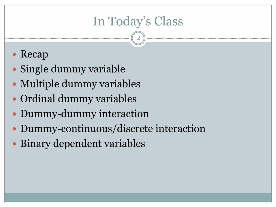
In Today’s Class2

Recap

Single dummy variable

Multiple dummy variables

Ordinal dummy variables

Dummy-dummy interaction

Dummy-continuous/discrete interaction

Binary dependent variables

Qualitative Information

Examples: gender, race, industry, region, rating grade, …

A way to incorporate qualitative information is to use dummy variables

They may appear as the dependent or as independent variables

A single dummy independent variable

Dummy variable:=1 if the person is a woman=0 if the person is man

= the wage gain/loss if the personis a woman rather than a man (holding other things fixed)

Introducing Dummy Independent Variable

Graphical Illustration

Alternative interpretation of coefficient:

i.e. the difference in mean wage betweenmen and women with the same level ofeducation.

Intercept shift

Illustrative Example

Dummy variable trapThis model cannot be estimated (perfect collinearity)

When using dummy variables, one category always has to be omitted:

Alternatively, one could omit the intercept:

The base category are men

The base category are women

Disadvantages:1) More difficult to test for diffe-rences between the parameters2) R-squared formula only validif regression contains intercept

Specification of Dummy Variables

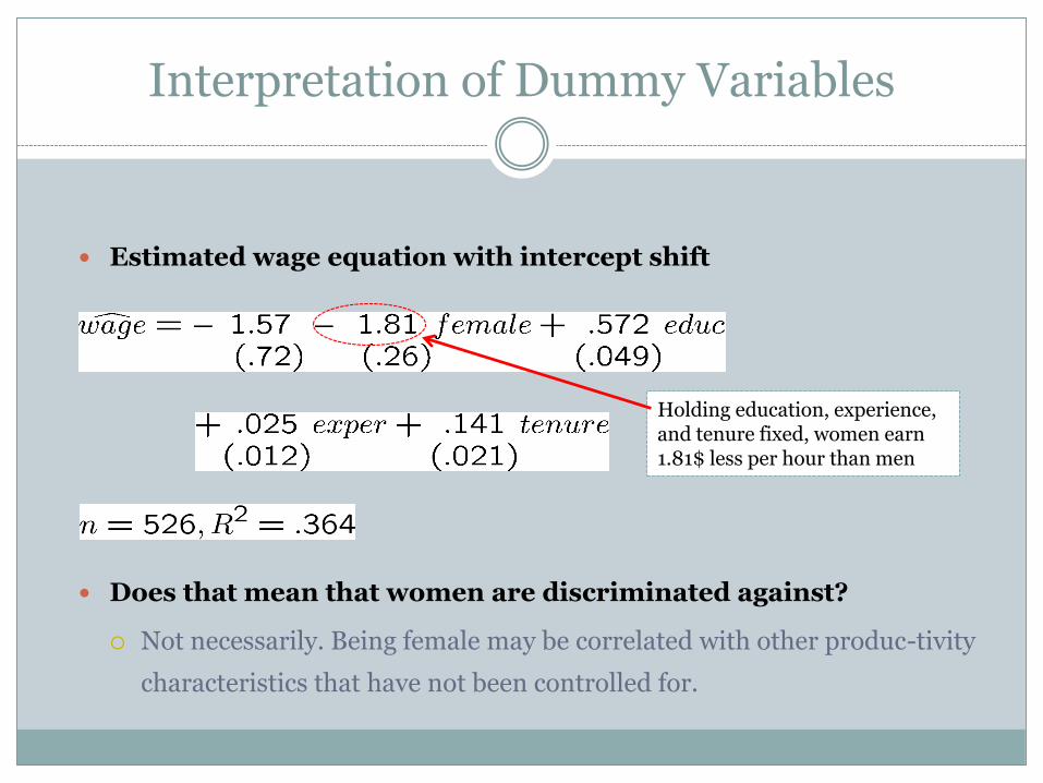
Estimated wage equation with intercept shift

Does that mean that women are discriminated against?

Not necessarily. Being female may be correlated with other produc-tivity

characteristics that have not been controlled for.

Holding education, experience, and tenure fixed, women earn1.81$ less per hour than men

Interpretation of Dummy Variables

Comparing means of subpopulations described by dummies

Discussion

It can easily be tested whether difference in means is significant

The wage difference between men and women is larger if no other things

are controlled for; i.e. part of the difference is due to differ-ences in

education, experience and tenure between men and women

Not holding other factors constant, womenearn 2.51$ per hour less than men, i.e. thedifference between the mean wage of menand that of women is 2.51$.

Model with only dummy variables-(Example-1)

Further example: Effects of training grants on hours of training

This is an example of program evaluation

Treatment group (= grant receivers) vs. control group (= no grant)

Is the effect of treatment on the outcome of interest causal?

Hours training per employee Dummy indicating whether firm received training grant

Model with only dummy variables-(Example-2)

Using dummy explanatory variables in equations for log(y)

Dummy indicatingwhether house is ofcolonial style

As the dummy for colonialstyle changes from 0 to 1, the house price increasesby 5.4 percentage points

Dependent log(y) and Dummy Independent

Holding other things fixed, marriedwomen earn 19.8% less than singlemen (= the base category)

Using dummy variables for multiple categories

1) Define membership in each category by a dummy variable

2) Leave out one category (which becomes the base category)

Dummy variables for multiple categories

Incorporating ordinal information using dummy variables

Example: City credit ratings and municipal bond interest rates

Municipal bond rate Credit rating from 0-4 (0=worst, 4=best)

This specification would probably not be appropriate as the credit rating only containsordinal information. A better way to incorporate this information is to define dummies:

Dummies indicating whether the particular rating applies, e.g. CR1=1 if CR=1 and CR1=0 otherwise. All effects are measured in comparison to the worst rating (= base category).

Ordinal Dummy Variables

Interactions involving dummy variables

Allowing for different slopes

Interesting hypotheses

= intercept men

= intercept women

= slope men

= slope women

Interaction term

The return to education is thesame for men and women

The whole wage equation isthe same for men and women

Interactions among dummy variables

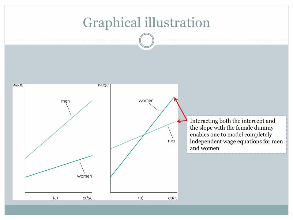
Interacting both the intercept andthe slope with the female dummyenables one to model completelyindependent wage equations for menand women

Graphical illustration

Estimated wage equation with interaction term

No evidence against hypothesis thatthe return to education is the same for men and women

Does this mean that there is no significant evidence oflower pay for women at the same levels of educ, exper, and tenure? No: this is only the effect for educ = 0. Toanswer the question one has to recenter the interactionterm, e.g. around educ = 12.5 (= average education).

Dummy-Continuous /Discrete Interaction (1)

Testing for differences in regression functions across groups

Unrestricted model (contains full set of interactions)

Restricted model (same regression for both groups)

College grade point average Standardized aptitude test score High school rank percentile

Total hours spentin college courses

Dummy-Continuous /Discrete Interaction (2)

Null hypothesis

Estimation of the unrestricted model

All interaction effects are zero, i.e. thesame regression coefficients apply tomen and women

Tested individually, the hypothesis thatthe interaction effectsare zero cannot berejected

Dummy-Continuous /Discrete Interaction (3)

Joint test with F-statistic

Alternative way to compute F-statistic in the given case

Run separate regressions for men and for women; the unrestricted SSR is

given by the sum of the SSR of these two regressions

Run regression for the restricted model and store SSR

If the test is computed in this way it is called the Chow-Test

Important: Test assumes a constant error variance accross groups

Null hypothesis is rejected

Restricted and Unrestricted Models (with Dummy Variables)

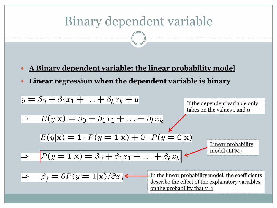
A Binary dependent variable: the linear probability model

Linear regression when the dependent variable is binary

Linear probabilitymodel (LPM)

If the dependent variable onlytakes on the values 1 and 0

In the linear probability model, the coefficientsdescribe the effect of the explanatory variables on the probability that y=1

Binary dependent variable

Does not look significant (but see below)

Example: Labor force participation of married women

=1 if in labor force, =0 otherwise Non-wife income (in thousand dollars per year)

If the number of kids under sixyears increases by one, the pro-probability that the womanworks falls by 26.2%

Binary dependent variable:Example-1

Example: Female labor participation of married women (cont.)

Graph for nwifeinc=50, exper=5, age=30, kindslt6=1, kidsge6=0

Negative predicted probability but no problem because no woman in the sample has educ < 5.

The maximum level of education in the sample is educ=17. For the gi-ven case, this leads to a predictedprobability to be in the labor forceof about 50%.

Binary dependent variable:Example-2

Disadvantages of the linear probability model

Predicted probabilities may be larger than one or smaller than zero

Marginal probability effects sometimes logically impossible

The linear probability model is necessarily heteroskedastic

Heterosceasticity consistent standard errors need to be computed

Advantanges of the linear probability model

Easy estimation and interpretation

Estimated effects and predictions often reasonably good in practice

Variance of Ber-noulli variable

Disadvantages: Linear probability model

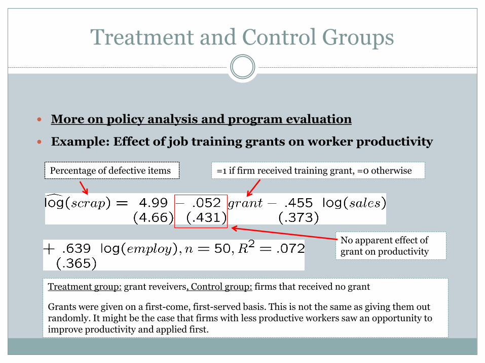
More on policy analysis and program evaluation

Example: Effect of job training grants on worker productivity

Percentage of defective items =1 if firm received training grant, =0 otherwise

No apparent effect ofgrant on productivity

Treatment group: grant reveivers, Control group: firms that received no grant

Grants were given on a first-come, first-served basis. This is not the same as giving them out randomly. It might be the case that firms with less productive workers saw an opportunity toimprove productivity and applied first.

Treatment and Control Groups

Self-selection into treatment as a source for endogeneity

In the given and in related examples, the treatment status is probably

related to other characteristics that also influence the outcome

The reason is that subjects self-select themselves into treatment

depending on their individual characteristics and prospects

Experimental evaluation

In experiments, assignment to treatment is random

In this case, causal effects can be inferred using a simple regression

The dummy indicating whether or not there was treatment is unrelated to other factors affectingthe outcome.

Self Selection and Endogeneity

Further example of an endogenuous dummy regressor

Are nonwhite customers discriminated against?

It is important to control for other characteristics that may be important

for loan approval (e.g. profession, unemployment)

Omitting important characteristics that are correlated with the non-

white dummy will produce spurious evidence for discriminiation

Dummy indicating whetherloan was approved

Racedummy

Credit rating

Endogenuous dummy regressor