Lecture 7

Genetic DriftBruce Walsh. jbwalsh@u.arizona.edu. University of Arizona.Notes from a short course taught June 2006 at University of Aarhus

The notes for this lecture were last corrected on 23 June 2006. Please email me any errors.

Finite population size results in random changes in allele frequencies. Lecture 3 briefly introducedgenetic drift on a single locus. Here we greatly expand upon these results, building up a neutraltheory for both single loci and also for neutral drift in phenotypes. These will serve as null modelsfor tests of selection. Lecture 8 considers using molecular data to look for signatures of selection atindividual loci, while Lecture 15 looks at tests of selection versus drift in accounting for a patternof long-term phenotypic evolution.

SINGLE LOCUS THEORY OF RANDOM GENETIC DRIFT

When the population is finite and stable, N individuals produce N offspring. This requires the Nparents to produce the 2N gametes that form this next generation. This produces random changesin allele frequencies (Figure 7.1), with this random drift being more dramatic in smaller populationsizes. The classic model for this is the Wright-Fisher model of genetic drift.

Figure 7.1. Random genetic drift. Starting with an allele A at frequency 0.5, eventually half of the lines willlose A, while the other half with fix A.

The Wright-Fisher Model of Genetic Drift

Suppose there are i copies of allele A in generation t. Thus the allele frequency is

p(t) =i

2N(7.1)

The Wright-Fisher model assumes that all parents produce a very large number of gametes, andoffspring are produced by random draws from this gamete pool. Hence, p(t) is the probability thatany single draw is anA allele, so that the total number ofA alleles drawn for the offspring follows a

Lecture 7, pg. 1

binomial distribution. Hence, the probability that the new frequency is p′j = j/(2N) given that thecurrent frequency is pi = i/(2N) is just

Pr(i copies→ j copies) =2N !

(2N − j)!j!

(i

2N

)j (2N − i2N

)2N−j(7.2)

For example, the probabilty that allele A is fixed in the next generation is just

Pr(j = 2N) = p2N =(

i

2N

)2N

(7.3a)

while the probabilty that A is lost in a single generation is

Pr(j = 0) = (1− p)2N =(

1− i

2N

)2N

(7.3a)

The net result of this binomial sampling is that the mean change in allele frequency is zero (ifthe current frequency is p, the expected frequency in the next generation is also p). However, thevariance in the change in allele frequency is p(1− p)/2N . Summarizing,

E(∆p|p) = 0, σ2(∆p) =p(1− p)

2N(7.4)

This sampling generates a random walk, a walk that stops when the allele being followed reachesfrequency zero (allele is lost) or one (allele is fixed). Two quantities of interest are the probability offixation and the expected time to fixation. Diffusion theory (discussed below) allows us to obtainboth of these quantities, not only for pure drift but also with drift and selection.

For a neutral allele, the probability of fixation U(p) only depends on the initial allele frequencyp, as

U(p) = p under pure drift (7.5)

Likewise, starting with a single copy, the expected time to fixation (for those alleles that are destinedto become fixed) is 4N . Similarly, the expected time for an allele introduced as a single copy to belost is ln(N).

Example 7.1. Suppose population is size 1000, and a single mutation a arises. If this is selectivelyneutral, its probability of fixation is

U

(1

2000

)=

12000

= 0.0005

In such cases, the expected time to fixation is 4N = 4,000 generations. In most cases, this mutationis lost, which occurs with probability 0.9995. In such cases, the mean time that the allele presists isln(N) = ln(1000) = 6.9 generations. If the population size was instead 107, then this allele is almostalways lost, but its persistance time increases to ln(107) = 16 generations.

Thus, the effect of drift is to remove variation by choosing a random allele and fixing it at theexpense of all other alleles. We can also view this in another, very powerful, way. As drift occurs,we lose lineages, so that eventually all of the copies on the population trace back to a single ancestralcopy. Thus, drift generates inbreeding. We also can speak of the lineages coalescing to a singlelineage (line of descent), and the result pattern of how the lineages coverge back in time is calledthe coalescent process. We will dealing with inbreeding first before examining the coalescent.

Lecture 7, pg. 2

Inbreeding and Drift

Under the Wright-Fisher model of drift, each individual produces the same (very large) number ofgametes, and we randomly sample from this pool to form the next generation. Thus, the chance ofdrawing 2 copies of the exact same allele from a particular parent (i.e., the copies are IBD) is just1/(2N), as once we draw the first copy, there is a 1/(2N) chance that we redraw the same allele.Otherwise (Probability 1− 1/[2N ]) we draw another random allele. If the population is not inbred,this random allele is not IBD, while if the population is inbred, then the chance that it is also IBD isf(t). Hence, with finite population size, inbreeding accumulates according to the recursion equation

f(t) =1

2N+(

1− 12N

)f(t− 1) (7.6)

Subtracting both sides from 1, this simplifies to the recursion formula

1− f(t) =(

1− 12N

)[1− f(t− 1)] (7.7a)

which generalizes to

1− f(t) =(

1− 12N

)t[1− f(0)] (7.7b)

Note that as t → ∞, [1 − f(t)] → 0 at a rate that is inversely proportional to population size.Individuals are expected to become completely inbred at loci that are unmodified by selection,mutation, and migration.

Recall that [1− f(t)] is the expected heterozygosity (Ht) relative to that in the base population(H0). From Equation (7.7b) we see that after t generations at a constant population size N,

Ht =(

1− 12N

)tH0 (7.8)

whereH0 is the initial heterozygosity. This rate of decay of heterozygosity of 1/2N was first obtainedby Wright (1931) using a rather different approach. It may be of interest to the non-mathematicallyinclined that Fisher, an excellent mathematician, obtained the wrong answer in 1922.

This loss of heterozygosity can be quantified using an exponential approximation to Equation7.8. Since (1− x)t ' exp(−xt) for |x| << 1,

Ht ' H0 exp(−t/2N) (7.9)

This can be solved to show that the heterozygosity is reduced to half ofH0 in about 1.4N generationsand to 5% of H0 in about 6N generations. If the population size is variable, Equation 7.8 becomes

Ht = H0

t∏i=1

(1− 1

2Ni

)(7.10)

where the∏

sign denotes a product of terms. This expression illustrates an important point. Eachof the terms, [1 − (1/2Ni)], is necessarily less than one. Thus, an expansion of population size canonly reduce the rate of erosion of heterozygosity; it cannot eliminate it.

The Coalescent Process for Drift

As mentioned, one powerful way to think about genetic drift is to consider the ancestral origins ofalleles in a population. Under drift, one can eventually trace all existing alleles in a population back

Lecture 7, pg. 3

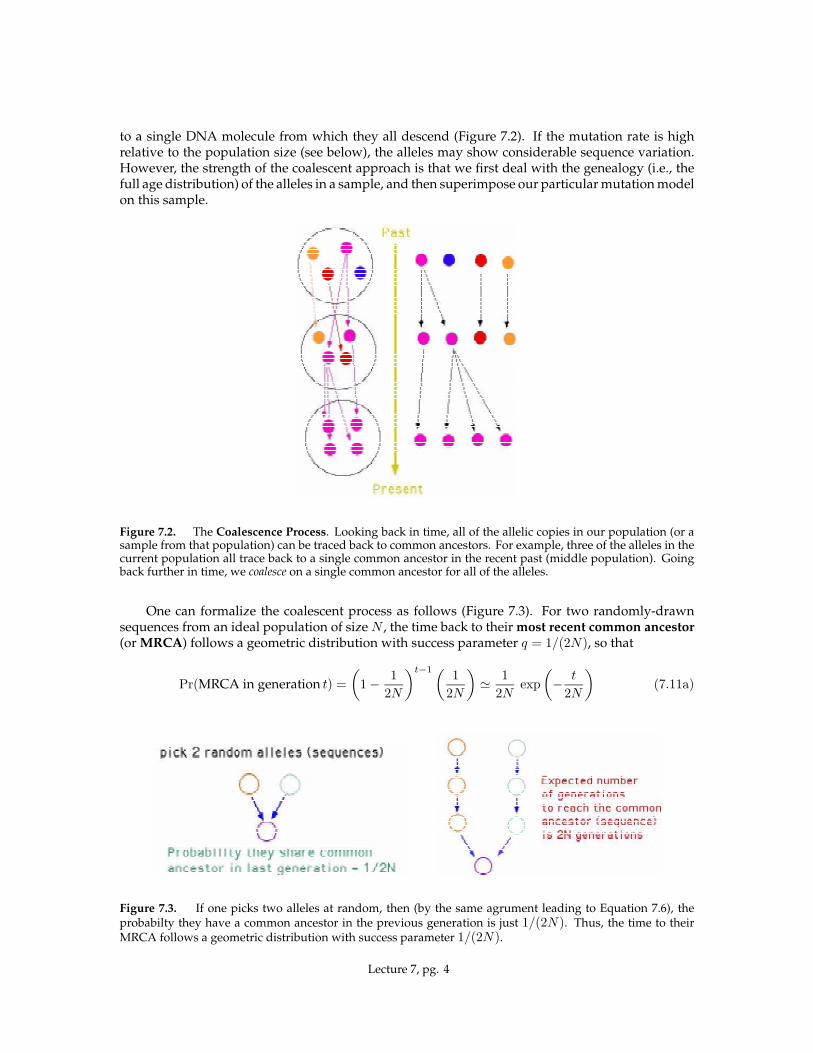
to a single DNA molecule from which they all descend (Figure 7.2). If the mutation rate is highrelative to the population size (see below), the alleles may show considerable sequence variation.However, the strength of the coalescent approach is that we first deal with the genealogy (i.e., thefull age distribution) of the alleles in a sample, and then superimpose our particular mutation modelon this sample.

Figure 7.2. The Coalescence Process. Looking back in time, all of the allelic copies in our population (or asample from that population) can be traced back to common ancestors. For example, three of the alleles in thecurrent population all trace back to a single common ancestor in the recent past (middle population). Goingback further in time, we coalesce on a single common ancestor for all of the alleles.

One can formalize the coalescent process as follows (Figure 7.3). For two randomly-drawnsequences from an ideal population of size N , the time back to their most recent common ancestor(or MRCA) follows a geometric distribution with success parameter q = 1/(2N), so that

Pr(MRCA in generation t) =(

1− 12N

)t−1( 12N

)' 1

2Nexp

(− t

2N

)(7.11a)

Figure 7.3. If one picks two alleles at random, then (by the same agrument leading to Equation 7.6), theprobabilty they have a common ancestor in the previous generation is just 1/(2N). Thus, the time to theirMRCA follows a geometric distribution with success parameter 1/(2N).

Lecture 7, pg. 4

The mean coalescence time is E[t] = 2N generations with variance σ2(T ) = 4N2. Hence, theprobability that two randomly-chosen alleles have a common ancestor within the last τ generationsis

1− Pr(no common ancestor in last τ generations) = 1− (1− q)τ (7.11b)

The Coalescent for a Sample

One very powerful feature of the coalescent process is that it is easy to apply to samples from aWright Fisher process. This in turn allows us to compute expected values and sampling variances(used in Lecture 8) under various mutation models. We have already seen that the coalescent time(the time to the MRCA) for a pair of random alleles follows a geometric distribution with successparameter q = 1/(2N). Suppose instead that we have a sample of size n and wish to know thefirst coalescent time, namely the time back to the closest common ancestor for the two most closelyrelated alleles in the sample. There are n choose 2, or n(n−1)/2 combinations, each with probability1/(2N), giving this time as being geometrically distributed with success parameter

qn =n(n− 1)

4N(7.12a)

Hence, the probability that the sampled alleles have at least one coalescent in the last τ generationsis just

1− (1− qn)τ (7.12b)

and likewisePr(first coalescent in generation t) = (1− qn)tqn ' qne−tqn (7.12c)

Similarly, once we have the time to the first coalescent, the time until the second for our sample isjust given by

qn−1 =(n− 1)(n− 2)

4N

In general, the time from the j − 1 to the jth coalescence has success parameter

qj =j(j − 1)

4N(7.12d)

Since the mean time for a geometric is 1/q, the mean time until k coalescences have occurred is just

4N(

1n(n− 1)

+1

(n− 1)(n− 2)+ · · ·+ 1

(n− k + 1)(n− k)

)(7.12e)

Likewise, the mean time until all of the alleles in the sample coalesce is just

4Nn∑i=2

1i(i− 1)

(7.12e)

The sum approaches 1 for large n, giving the MRCA for the entire sample as roughly 4N. Forexample, for n = 2, 5, 10, 25, 50, the sum has value 0.5, 0.8, 0.9, 0.96, and 0.98. As well will see inLecture 8, various mutational models under the Wright-Fisher process involves terms of 1/i and1/i2. Equations 7.12d-e motivates the general form of these expressions.

Lecture 7, pg. 5

t5

t4

t3

t2

Figure 7.4. The coalescence for a sample of 5 alleles from a population of size N . Time runs from the present(bottom) to the past (top). Here t5 is the time back until the first coalescence, which follows a geometricdistribution with success parameter 5(5− 1)/(4N) = 5/N , for a mean time ofN/5. Likewise, t4 has a meanof N/3, giving a mean time for the first two coalescences to occur as (1/5 + 1/3)N = (6/15)N . Similarly, themean for t3 and t2 are (2/3)N and 2N , respectively, giving the total mean time for these five alleles to coalesceas 3.2N .

Drift Generates Between-Population Variance in Replicate Lines

While drift removes variation within a line, it increases the variance between replicate lines. Supposewe have a large number of replicate lines all initially with frequency p0 for allele a. Eventually p0

of the lines are fixed for allele a, while 1 − p0 lose this allele. Setting X as the random variable forallele frequency, we then have

X ={

1 with probability p0

0 with probability 1− p0

Taking the appropriate expectations of X gives the between-line variance as

σ2(X) = E(X2)− [E(X)]2 = 12 · p0 − (1 · p0)2 = p0(1− p0) (7.13)

More generally, the variance in gene frequency in generation t is

σ2p(t) = E(p2

t )− E2(pt)

Adding and subtracting E(pt),

σ2p(t) = [E(pt)− E2(pt)] + [E(p2

t )− E(pt)]= E(pt)[1− E(pt)]− E[pt(1− pt)]

Because there are no systematic forces causing the gene frequency to increase or decrease,E(pt) = p0,and the first quantity on the right is p0(1 − p0). The quantity E[pt(1 − pt)] is half the expectedheterozygosity in a population in generation t. Recalling Equation (7.8),

σ2p(t) = p0(1− p0)

[1−

(1− 1

2N

)t](7.14a)

which is well approximated by

σ2p(t) ' p0(1− p0)[1− exp(−t/2N)] (7.14b)

Lecture 7, pg. 6

EFFECTIVE POPULATION SIZE, Ne

Up to now, we have assumed a randomly mating population, constant in size, with equal sex ratiosand roughly equal offspring contribution from each parent. Such ideal populations are unlikely innature, but fortunately we can construct a surrogate index that takes into account the deviationsfrom the ideal model. Such an index has become widely known as Ne, the effective population size,following the early and influential work of Wright (1931, 1938, 1939).

It is important to note that N enters into drift in two ways. The first (Equation 7.4) is that thesampling variance under the Wright-Fisher model is p(−1p)/(2N). Adjustments for depatures froman ideal population here generates the variance effective population size. The second (Equation7.6) is that inbreeding accumulates at a rate of 1/(2N), and adjustments here generate the inbreedingeffective population size. These are often very similar, and our results below refer to inbreedingeffective population size.

Ne With Variable Population Size

From Equations 7.8 and 7.10, the effective population size with variable population size satisfies

(1− 1

2Ne

)t=

t∏i=1

(1− 1

2Ni

)

An excellent approximation can be obtained by once again (1− x)t ' exp(−tx) and likewise

(1− x1)(1− x2) · · · (1− xt) ' exp

(−

t∑i=1

xi

)

Thus we havet

2Ne=

t−1∑i=0

12Ni

which has solution

Ne =t

t∑i=1

1Ni

=t

1N1

+1N2

+ · · ·+ 1Nt

(7.15)

The long-term effective sizeNe is thus approximately equal to the harmonic mean of the populationsizes.

Example 7.2. Population bottlenecks have especially pronounced effects on Ne. Suppose the popu-lation cycles between values of 10000,10000,10000, and 10. The average population size in this case isslightly over 7,500. However, the harmonic mean

Ne =4

110000

+1

10000+

110000

+1

100

= 399

Lecture 7, pg. 7

Ne With Unequal Sex Ratios

Unequal sex ratios can also have a dramatic effect on the effective population size. In particular, ifthere are Nm males and Nf females, then

Ne =4NmNfNm +Nf

(7.16)

Example 7.3. Suppose we have 1000 female salmon, and use 2 males to fertilize all of their eggs.The resulting effective population size becomes

Ne =4 · 1000 · 2

1002= 8

Ne With Unequal Offspring Contribution

Individuals, on average, contribute different number of offspring to the next generation. For exam-ple, the 2 male salmon above might have left 50 and 1500 offspring, respectively. One might expectthat this gives a smaller Ne than if they contributed essentially the same number of offspring. Thisthought is indeed correct, and we formalize it here. Let µo be the mean number of gametes that aparent contributes to the next generation (µo = 2 for a population in steady-state, as each parentalpair replaces itself, which requires two gametes from each) and let σ2

o be the variance in gameticcontribution. Then

Ne '2N

σ2o/µo + 1

(7.17)

One common model is for parents to contribute, on average, two offspring (for a replacement ofthe male and female parent), with offspring number given by a Poisson distribution with mean 2(this means each parent has the same chance as any other parent of leaving offspring). In this case,µo = σ2

o = 2 and Ne ' N . However, suppose we force the population so that each parent leavesexactly one male and one female. In this case, σ2

o = 0 and Ne = 2N . This is a rare case where theeffective population size is larger than the actual population size.

In a summary of data on lifetime reproductive success in birds, Grant (1990) found that σ2o/µo

ranged from 1.2 to 4.2, which is much greater than the ratio of 1 expected under the Poisson offspringmodel. Substituting into Equation 7.17, the effective female population size for these species is 40-90% of the actual number of females. We expect the variance in male reproductive success to beeven larger, as it is typically the case that a few males get a disproportionate number of females,and a significant number of males have no mates.

MUTATION-DRIFT EQUILIBRIUM: SINGLE LOCI

As mentioned, drift removes variation, while mutation introduces it. Since any finite populationwill experience both forces (and perhaps others, such as selection and migration), the joint effectsof these two opposing forces is of much interest.

Within-Population Equilibrium Variance

A classic result from theoretical population genetics is Kimura and Crow’s (1964) infinite allelesmodel. This paper started the field of molecular population genetics, as the assumed mutationalmodel for this model was motivated by DNA structure. When considering the DNA sequence of agene, it is not unreasonable to assume that each new mutation gives rise to an allele never beforepresent in the population, as each new mutation likely occurs in a different base pair. Thus, there

Lecture 7, pg. 8

are an infinite number of possible alleles. In this case, the measure of standing variation is simplypopulation heterozygosity. In a very small population, almost everyone should be a homozygote.However, if the population and (and/or mutation rate) is sufficiently large, then there will be lotsof alleles and hence a high frequency of heterozygous.

This was indeed shown, as Kimura and Crow found that the equilibrium heterozygosity wasgiven by

H =4Neµ

4Neµ+ 1(7.18)

whereNe is the effective population size and µ the mutation rate to new alleles. As shown in Figure7.5, when 4Neµ is large, there is lots of variation, withH close to one when 4Neµ >> 1. Conversely,when 4Neµ is small, the population shows little genetic variation, with H = 4Neµ << 1.

Figure 7.5. Equilibrium level of heterozygosity under Crow and Kimura’s infinite alleles model.

Coalescent theory provides an easy way see that 4Neµdetermines the amount of heterozygosity.Suppose we draw two sequences at random. On average, how many mutations should they differby? As shown in Figure 7.6, if the two sequences have a common ancestor t generations ago, theexpected number of mutational difference between then (under the infinite alleles model) is 2tµ.

Figure 7.6. If the time back to a common ancestor to two sequences being compared is t generations, thena total divergence of 2t separates the pair. If µ is the per-generation mutation rate, the expected number ofmutations is 2tµ.

The actual number of mutations follows a Poisson distribution with mean 2tµ, so that the probabilitythe sequences differ by k mutations is

Pr(k) =(2tµ)ke−2tµ

k!(7.19)

Lecture 7, pg. 9

Coalescent theory tells us that the average time back to a common ancestor for two alleles is t = 2Ne,giving the expected number of mutations between two random sequences as 2tµ = 4Neµ. If4Neµ > 1, we expect, on average, at least one mutational difference between two random alleles,and we would score this individual as a heterozygote. If 4Neµ << 1, we except most pairs ofsequences to show no mutational differences, and hence be scored as a homozygote.

Divergence Between Populations

One consequence of drift fixing segregating alleles and mutation introducing new alleles is thatthe DNA sequences of two isolated populations drift apart by substituting different mutations. Wehave already see (Equation 7.13) that random fixation of the initial common variation generatesan eventual between-replicate-line variance of p0(1 − p0), where p0 is the initial allele frequency.This variance generated by the distribution of the initial heterozygosity is usually ignored whenconsidering long periods of divergence, as the variance generated by mutation dominates.

While the standing heterozygosity under drift and mutation is a function of the product ofmutation rate and population size (Equation 7.18), the rate at which populations divergence underdrift is just a function of the mutation rate µ. To see this, note that the expected substitution rate pergeneration is given by

( Number of new mutations per generation ) * ( Prob of fixation of a single new mutation)

2Nµ ·(

12N

)= µ (7.20)

The role of the actual population size N exactly cancels. Larger populations give rise to moremutations (2Nµ), but each new mutation has a smaller chance of fixation (1/[2N ]). Thus, the rate ofdivergence under drift is independent of the population size. For population that have been separated fort generations, the expected divergence (number of mutations) d is just

d = 2tµ (7.21)

Note that the per generation substitution rate refers to the rate at which new alleles (destined tobecome fixed) arise. Once such a destined allele arises by mutation, it still must become fixed (Figure7.7). Hence, we need to distinguish between the time to fixation and the time between appearanceof new mutants destined to become fixed. From our previous results, the time to fixation given westart with a single copy is 4N generations, while the expected waiting time for a new successful(destined to be fixed) mutation to appear is a geometric with success parameter µ. Hence, the meantime for their apperance is 1/µ.

Figure 7.7. The waiting time between successful new mutations vs. the actual time to fix such a mutation.

Lecture 7, pg. 10

The key biological point from Equations 7.18 and 7.21 is that the interaction of drift and mutationgenerates both polymorphism and substitution of alleles.

Kimura’s Neutral Theory of Molecular Evolution

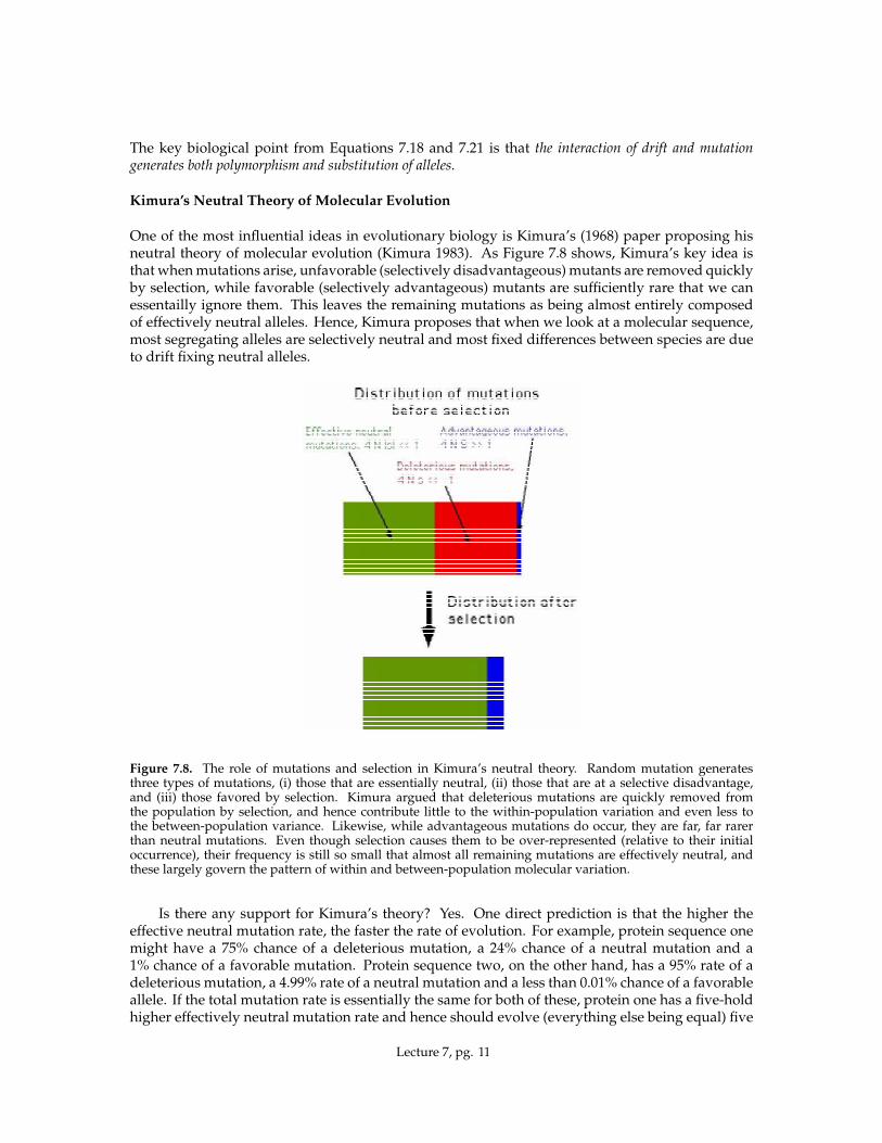
One of the most influential ideas in evolutionary biology is Kimura’s (1968) paper proposing hisneutral theory of molecular evolution (Kimura 1983). As Figure 7.8 shows, Kimura’s key idea isthat when mutations arise, unfavorable (selectively disadvantageous) mutants are removed quicklyby selection, while favorable (selectively advantageous) mutants are sufficiently rare that we canessentailly ignore them. This leaves the remaining mutations as being almost entirely composedof effectively neutral alleles. Hence, Kimura proposes that when we look at a molecular sequence,most segregating alleles are selectively neutral and most fixed differences between species are dueto drift fixing neutral alleles.

Figure 7.8. The role of mutations and selection in Kimura’s neutral theory. Random mutation generatesthree types of mutations, (i) those that are essentially neutral, (ii) those that are at a selective disadvantage,and (iii) those favored by selection. Kimura argued that deleterious mutations are quickly removed fromthe population by selection, and hence contribute little to the within-population variation and even less tothe between-population variance. Likewise, while advantageous mutations do occur, they are far, far rarerthan neutral mutations. Even though selection causes them to be over-represented (relative to their initialoccurrence), their frequency is still so small that almost all remaining mutations are effectively neutral, andthese largely govern the pattern of within and between-population molecular variation.

Is there any support for Kimura’s theory? Yes. One direct prediction is that the higher theeffective neutral mutation rate, the faster the rate of evolution. For example, protein sequence onemight have a 75% chance of a deleterious mutation, a 24% chance of a neutral mutation and a1% chance of a favorable mutation. Protein sequence two, on the other hand, has a 95% rate of adeleterious mutation, a 4.99% rate of a neutral mutation and a less than 0.01% chance of a favorableallele. If the total mutation rate is essentially the same for both of these, protein one has a five-holdhigher effectively neutral mutation rate and hence should evolve (everything else being equal) five

Lecture 7, pg. 11

times as fast. The message from this example is that sequences under the least selective constraint shouldbe evolving the fastest. This is indeed seen. Noncoding sequences and pseudogenes (nonfunctionalgenes) evolve at the fastest rate, while synonymous third-base positions (those that do not resultin a chance in the protein sequence) have the next highest rate, while non-synonymous changes(those that change the protein sequence) evolve at the slowest rates.

Additional support for the neutral theory comes form its ability to explain molecular clocks(Figure 7.9). If one takes a protein and plots the divergence between species pairs as a function of thedivergence time for those pairs, the data are very well fitted by a straight line, i.e., d = αt, divergenceis proportion to time. While proteins generally show this feature, different proteins differ in theirslopes (the rate α for the divergence per unit time). How can we jointly explain both the clock-likebehavior of a given protein as well as the difference in rate between different proteins?

The answer is that the neutral theory gives us Equation 7.21, d = 2tµ. Here, µ is really theneutral mutation rate. Hence we have clock-like divergence, with the rate given by the effectiveneutral mutation rate. From our discussion above, we expect less-constrained proteins to evolvethe fastest. This is indeed what is generally seen.

Figure 7.9. Protein clocks. Proteins tend to show linear divergence over time, but the rate differs over proteins.Here divergence is plotted versus time in such a way that the smaller (flatter) slopes evolve at higher rates.

A final deep implication of the neutral theory is that the rates of molecular and morphologicalevolution can become decoupled. An excellent example of this can be seen by comparing molecularand morphological features of frogs versus mammals. As a group, frogs are twice as old, and henceshow twice as much molecular variation. However, as a group, mammals show huge differencesin morphology, while frogs show rather little.

Property Frogs sNumber of Species 2050 4600Number of Orders 1 16-20Age of Group 150 MYr 77 MYrRate of Morphological slow fast

evolutionRate of Molecular standard standard

evolution

Lecture 7, pg. 12

MUTATION-DRIFT EQUILIBRIUM: ADDITIVE VARIANCE

We now consider the effects of drift on complex traits, which shifts our focus from heterozygosity ata single locus to the additive genetic variance. Recall from Equation 3.33a that the additive varianceis given by

σ2A = 2p (1− p)a2[ 1 + k ( 2p− 1 ) ]2

Our focus will be on the case with no dominance (d = 0). Here, σ2A = 2p (1 − p)a2, so that the

additive variance is a simple function of the heterozygosity, 2p(1 − p). Recalling Equation 7.9,Ht ' H0 exp(−t/2N), it immediately follows that

σ2A(t) = σ2

A(0) exp(−t/2N) (7.22)

Hence, with no dominance, the effect of drift is a monotonic reduction in the additive variance overtime, until all of the initial variation is lost. When dominance is present (d 6= 0), the behavior of σ2

A

under inbreeding (drift) can be much more complex. While the additive variance will eventuallydecline to zero, it may actually increase for a time. This can occur when rare recessives contributingto the trait increase in frequency under drift, increasing the additive variance for a time.

Likewise, the between-population variance (the variance in the means of replicate lines) followsby noting that the value when a contributing locus is fixed is

X ={

2a with probability p0

0 with probability 1− p0

giving the ultimate between-line variance as

σ2(X) = E(X2)− [E(X)]2 = 4a2 · p0 − (2a · p0)2 = 4a2p0(1− p0) = 2σ2A(0) (7.23a)

Hence, the between-line variance from drift partitioning the initial variance eventually approachestwice the initial additive variance. More generally (following Equation 7.14b), the between-linevariance at generation t is given by

σ2B(t) = 2σ2

A(0)[1− exp(−t/2N)] (7.23b)

Thus, in the absence of mutation, drift removes all of the additive variation within a population.The lost of this variation due to fixation within a line translates into a between-line variance thatapproaches twice the initial additive variation as all initial alleles become fixed.

Equilibrium Additive Variance Within a Population

Equations 7.22 and 7.23 describe the effects of drift alone. What happens when mutations occur?With quantitative traits, the mutation rate alone is not a sufficient descriptor, as we care about effectsize in addition to rate of occurrence. The result is that the mutational variance σ2

m describes themutation contribution to a complex trait. The variance can be estimated by looking at divergenceamong inbred lines or the response to selection in such lines. Empirically, a typical value (Lynchand Walsh 1998) for this variance is

σ2m ∼ 10−3σ2

E (7.24)

The dynamics of the within-population variance under drift and mutation is given by

σ2A(t+ 1) = σ2

m +(

1− 12Ne

)σ2A(t) (7.25)

Lecture 7, pg. 13

The first term is the contribution from new mutation, the second the fraction of the current additivevariation that is not removed by drift. At the mutation-drift equilibrium, σ2

A(t + 1) = σ2A(t) and

Equation 7.25 givesσ2A = 2Neσ2

m (7.26)

Starting with initial variation σ2A(0), the solution to Equation 7.25 in any particular generation is

σ2A(t) ' 2Neσ2

m +[σ2A(0)− 2Neσ2

m

]exp(−t/2Ne) (7.27)

The fraction of additive variation due to new mutation at time t is just

σ2A,m(t) ' 2Neσ2

m [ 1− exp(−t/2Ne) ] (7.28)

From Equation 7.26, the expected heritability at the mutation-drift equilibrium becomes

h2 =σ2A

σ2A + σ2

E

=2Neσ2

m

2Neσ2m + σ2

E

(7.29a)

which we can express as

h2 =2Neσ2

m∗2Neσ2

m∗ + 1, where σ2

m∗ =σ2m

σ2e

(7.29b)

Notice the similarity to the Kimura and Crow expression (Equation 7.18) for equilibrium heterozy-gosity.

Example 7.4. With σ2m = 10−3σ2

E and Ne = 2 for full sib inbreeding, σ2A at mutation-drift equilib-

rium is 4× 10−3σ2E , and the heritability is

h2 =σ2A

σ2A + σ2

E

=4× 10−3σ2

E

4× 10−3σ2E + σ2

E

= 0.004

which is trivial. For much larger population sizes, say Ne = 500,

σ2A = 1000× 10−3σ2

E and h2 =1000× 10−3σ2

E

1000× 10−3σ2E + σ2

E

= 0.5

The careful reader might note a problem with both Equations 7.18 (heterozygosity) and Equation7.29 (heritability). From Equation 7.24, a typical value assumed for σ2

m∗ is 10−3, and Equation 7.29bbecomes

h2 =2Ne

2Ne + 1000(7.30)

Thus, even for not terribly large Ne (say a couple of thousand), the expected heritability is close toone. The same in seen for expected heterozygosity in Equation 7.18, in that for very large populationswe also expect H to be close to one. Neither of these expectations are seen in large populations.Why is this the case?

One answer follows from the neutral theory and from the result (Equation 3.20) that an alleleunder selection (s) behaves as neutral allele when 4Ne| s | << 1 and as an allele under selectionwhen this product is >> 1. The mutation rate (and mutational variance) in Equations 7.18 and 7.29is the neutral variance. If some mutations have deleterious effects on fitness, these are not included.Note that as population size increases, so does 4Ne| s |, so that a higher fraction of new mutationsmay now be no longer effectively neutral, but rather under selection. Most of these are deleteriousand hence to not make any substantial contribution to the either the standing heterozygosity (H)or heritability (h2). Values of σ2

m are typically estimated from populations with very smallNe, suchas brother-sister mated lines. In such cases, alleles must have large effects on fitness in order for4Ne| s | >> 1 to be satisfied. However, if mutations affecting our trait of interest also have effectson fitness, then in larger populations these may be quickly removed by selection. Thus estimates ofσ2m should be viewed as overestimates of the value that contributes to Equations 7.26 - 7.29.

Lecture 7, pg. 14

Divergence Between Populations

Recall that random fixation of the initial alleles generates (Equation 7.23b) a variance between lines(i.e., the variance of the line means), ultimately reaching a final value of 2σ2

A. By contrast, mutationalinput continually generates an increasing variance between lines. The between-line variance (dueto mutation) in generation t is

σ2B,m(t) = 2σ2

m[ t− 2Ne(1− e−t/2Ne)] (7.31)

At equilibrium, the rate of divergence is 2σ2m per generation and the between-line variance ap-

proachesσ2B,m(t) ' 2tσ2

m (7.32a)

to which we can also add the contribution from the initial variance,

σ2B(t) ' 2tσ2

m + 2σ2A(0) (7.32b)

For sufficiently large t the mutation contribution dominates and so we typically use Equation 7.32a.Again note the parallels with our single-locus results. The amount of standing variation de-

pends on the product of mutation rate and population size (Equations 7.18 and 7.29), while thedivergence between populations simply depends on the product of mutation rate and divergencetime (Equation 7.21 and 7.32a), with population size not entering. Thus, the rate of divergence in traitmeans from drift is independent of the population size.

DIFFUSION THEORY

Diffusion theory refers to a set of mathematical machinery for dealing with fairly general classesof stochastic processes (such as those that occur in genetics). We review some of the key resultshere, which have applications to the dynamics of alleles under drift and other forces, and also toquantitative traits under drift (and possibly selection).

Consider a continuous random variable xt indexed by continuous time t. If δx = xt+δt − xt(the change in xt over a very small time interval δt) satisfies

E (δx |xt = x) = m(x)δt + o(δt)

σ2(δx |xt = x) = v(x)δt + o(δt)

E(|δx|k

)= o(δt) for k ≥ 3

then xt is said to be a diffusion process (provided the additional technical restriction that xt isa Markov process is satisfied). o(δt) means that the error term is small relative to δt (formally,limδt→0 o(δt)/δt = 0), whilem(x) and v(x) correspond to the mean and variance of the process overa very small time interval. The entire structure of a diffusion is thus described by m(x) and v(x),allowing analytic expressions for quantities of interest to be obtained, as we develop below.

Diffusion processes are of special importance in that a discrete space, discrete time, randomvariable can often be closely approximated by a diffusion. This is done by appropriately scalingof space and time to construct a new random variable. For example, consider Xt, the numberof copies of allele A in a discrete-generation population of N diploids at generation t. Xt takeson values 0, 1, . . . , 2N and time t is in discrete units of generations. Constructing a new randomvariable x(N)

τN = X(τN )/(2N), where τN = t/N — a single generation increments the new time scaleby 1/N . Taking the limit as N approaches infinity, the limiting process xτ is a continuous space,continuous time process that represents the allele frequency at time τ (e.g., limN→∞ xτN = pτ , the

Lecture 7, pg. 15

frequency at time τ ). If scaling is correctly done, xτ is now a diffusion process and provides a goodapproximation to the behavior of Xt. One immediate consequence of this scaling argument is thatthe process proceeds at a rate proportional to N . Hence, the larger N , the slower the rate.

Infinitesimal Means and Variances, m(x) and v(x)

The infinitesimal mean, m(x), and the infinitesimal variance, v(x), are formally defined by

m(x) = limδ→0

E (xt+δ − xt |xt = x)δ

(7.33a)

v(x) = limδ→0

E[ (xt+δ − xt)2 |xt = x ]δ

(7.33b)

Example 7.5. A diffusion process examining changes in allele frequencies in a diploid is typicallyobtained by setting v(x) = x(1 − x)/(2Ne) (the per generation variance in the change of allelefrequencies due to drift, Equation 7.4) and using the deterministic change in allele frequency form(x).A diffusion process approximating pure drift can be constructed by use of a suitable time scale (seeKarlin and Taylor 1981 for details) to give

m(x) = 0, v(x) =x(1− x)

2Ne(7.34)

wherex = freq(A). Similarly, consider additive selection when |s| is small, so thatW ' 1. In this caseEquation 3.19a reduces to ∆p ' sp(1− p), suggesting as an approximating diffusion over 0 < x < 1

m(x) = sx(1− x), v(x) =x(1− x)

2Ne(7.35)

Finally, consider arbitrary selection with constant fitnesses (with selection sufficiently weak such thatW ' 1) and forward and back mutation. Let ν be mutation rate from A to a, µ the mutation ratefrom a to A, and p = freq(A). A trick that will prove useful is Wright’s Formula, which allows thechange in allele frequency under selection (Equation 3.19a) to be written as

∆p =x(1− x)

2d ln(W )dx

Applying Wright’s formula (modified to include mutation) gives

m(x) =x(1− x)

2d ln(W )dx

+ (1− x)µ− xν

and again

v(x) =x(1− x)

2Ne(7.36)

Stationary Distributions

At equilibrium, the probability density function (which describes the frequency x of an allele at timet given it starts at frequency p0) does not change over time, e.g.,

∂ ϕ(x, t, p0)∂ t

= 0 (7.37)

Lecture 7, pg. 16

Such a distribution (if it exists) is called the stationary distribution and is denoted byϕ(x), showingno dependence on either time t or initial frequency p0. The stationary distribution is independentof the starting conditions: regardless of where the process starts in the interior of the diffusion, itconverges to the same distribution. ϕ(x, t, p0) can thus be decomposed into a transient and a station-ary part, ϕ(x, t, p0) = ϕ∗(x, t, p0) + ϕ(x), where the transient part satisfies limt→∞ ϕ∗(x, t, p0) = 0.Hence, that part of the distribution depending on the initial starting conditions decays away overtime leaving only the stationary distribution.

The stationary distribution satisfies

ϕ(x) =C

v(x)G(x)(7.38)

where G is defined by the indefinite integral

G(x) = exp[−2

∫ x m(y)v(y)

dy

](7.39)

C is a constant such that ϕ(x) integrates to one, so Equation 7.38 is a proper probability densityfunction. Note that

∫[v(x)G(x)]−1 dx may be infinite, in which case no stationary distribution

exists. This happens, for example, in the absence of mutation and migration where both boundariesare absorbing. Pure drift is one such case as when the allele frequency reaches either zero or one, itcannot change further (it is either fixed or lost), and hence these boundaries are absorbing.

Example 7.6. Consider pure drift. From Equation 7.34, m(x) = 0 and v(x) = x(1 − x)/(2Ne),giving

G(x) = exp[−4Ne

∫ x 0y(1− y)

dy

]= e0 = 1 (7.40)

and

ϕ(x) =2NeCx(1− x)

(7.41)

The only valid equilibrium distribution is ϕ(x) = 0 (e.g., C = 0), as∫ 0

1x−1(1− x)−1dx =∞. This

makes sense, as after sufficient time all populations are either at x = 1 or x = 0, with no populationsshowing 0 < x < 1. The resulting equilibrium distribution on this interval is zero.

Example 7.7. Compute the stationary distribution for the frequency of an allele at a diallelic locusexperiencing selection, mutation and drift. From Equation 7.36,∫ x m(y)

v(y)dy = 2Ne

∫ x y(1− y)(1/2)d ln(W )/dy + (1− y)µ − yν

y(1− y)dy

= Ne

∫ x d ln(W )dy

dy + 2Neµ∫ x 1

ydy − 2Neν

∫ x 11− y dy

= Ne ln(W ) + 2Neµ ln(x) + 2Neν ln(1− x)

Hence,

G(x) = exp[− 2

∫ x m(y)v(y)

dy

]= W

−2Nex−4Neµ (1− x)−4Neν

Applying Equation 7.38 gives

ϕ(x) = CW2Ne

x4Neµ−1 (1− x)4Neν−1 for 0 < x < 1 (7.42)

Lecture 7, pg. 17

a result first due to Wright (1931). Using interactive mathematical graphics packages (such as Math-ematica) is a very fruitful way to explore the behavior of Equation 7.42, as well as other stationarydistributions.

Probability of Fixation

When at least one boundary is absorbing, no stationary distribution exists. In such cases, oneimportant descriptor of the process is the probability of reaching one boundary before the other.The solution for u(p0), the probability of fixation of an allele, given initial frequency p0, is

u(p0) =

∫ p0

0G(x) dx∫ 1

0G(x) dx

(7.43a)

More generally, for any diffusion (regardless of the nature of the boundaries) the probability thatthe process reaches b before a, given it starts at p0 (where A ≤ a ≤ p0 ≤ b ≤ B with the diffusiondefined over A < x < B), is

ub,a(p0) =

∫ p0

aG(x) dx∫ b

aG(x) dx

(7.43b)

Example 7.8. Compute the probability of fixation of an allele at a diallelic locus experiencing additiveselection and drift. From Equation 7.34,

m(x) = sx(1− x), v(x) =x(1− x)

2Ne

implying

G(x) = exp[−4Nes

∫ x y(1− y)y(1− y)

dy

]= e−4Nesx

Thus, we recover Kimura’s equation (3.20)

u(p0) =1− e−4Nesp0

1− e−4Nes

Likewise, for pure drift, G(x) = 1 (Equation 7.40), giving

u(p0) =

∫ p0

01 dx∫ 1

01 dx

= p0

Finally, allowing for dominance, from Equation 3.19a (assuming W ' 1),

m(x) = sx(1− x)(1 + h(1− 2x) )

giving

G(x) = exp[−4Nes

∫ x y(1− y)(1 + h(1− 2y) )y(1− y)

dy

]= exp

[− 4Nesx(1 + h(1− x) )

]and hence

u(p0) =

∫ p0

0exp [−4Nesx(1 + h(1− x) ] dx∫ 1

0exp [−4Nesx(1 + h(1− x) ] dx

Lecture 7, pg. 18

DIFFUSION APPLICATIONS TO QUANTITATIVE CHARACTERS

When we shift our attention from individual alleles to the phenotype of a quantitative characterunder drift, diffusions now follow the mean phenotype instead of the frequency of an allele. Twowell studied diffusions, Brownian motion and the Ornstein-Uhlenbeck process, are especiallyuseful in this case.

Brownian Motion Model of Evolution

For Brownian motion, the diffusion over −∞ < x <∞ is given by

m(x) = a v(x) = b (7.44)

where b > 0. The general solution under Brownian motion starting at x0 is that xt is normallydistributed, with mean x0 + at and variance σ2

t = bt. There is no equilibrium solution, as theprocess converges to a normal with infinite variance (and infinite mean if a 6= 0).

Example 7.9. Lande (1976) used Brownian motion to approximate the change in the phenotypic meanfor a neutral character with constant additive genetic variance. There is no directional force to changethe mean, so a = 0. Assuming the character is strictly additive, the per generation sampling variancein the mean is σ2

A/Ne, which is used for b. Hence, at generation t, the distribution of phenotypicmeans is approximately normal with expected mean µ0 (the initial mean) and variance σ2

t = tσ2A/Ne.

One measure of how quickly phenotypic means drift is given by the minimum number of generationsrequired such that a random population has at least a 50% probability of being more that K standarddeviations from its initial mean. This is expressed as Pr(|xt − µ0| ≥ Kσz) = 0.5, where xt is themean of a randomly drawn population and σ2

z the phenotypic variance. Assuming Brownian motion,(xt − µ0)/σt is a unit normal random variable, hence

Pr(|xt − µ0| ≥ Kσz) = Pr[|xt − µ0|

σt≥ Kσz

σt

]= Pr

[|U | ≥ Kσz

σt

]= 0.5

For a unit normal U , Pr(|U | ≥ 0.675) = 0.5, giving Kσz/σt = Kσz/(σA√t/Ne) = 0.675. Upon

rearranging and substituting h2 = σ2A/σ

2z ,

t =K2Neh2 0.6752

' 2NeK2

h2(7.45)

For example, forNe = 10, a neutral character with heritabilityh2 = 0.5 requires 2×10×9/0.5 = 360generations until half the populations have phenotypic means more than three standard deviationsfrom their initial value.

Recall that drift also changes σ2A, with the assumption of a constant σ2

A being reasonable only fort < N (unless the initial variance is close to its mutation-drift equilibrium value). Alternatively, wecould assume that the population has been at its current size sufficiently long enough so that additivevariance is at its mutation-drift equilibrium value (Equation 7.26), σ2

A = 2Neσ2m. The distribution

of means now has expected variance

σ2t = 2tNeσ2

m/Ne = 2tσ2m (7.46)

Here, the expected time until 50% of the means exceed K standard deviations is obtained fromKσz/

√t 2σ2

m = 0.675. Since√

2 · 0.675 = 0.95, we round this up to one to simplify things. Theusing σ2

z = σ2A + σ2

E ,

t = K2 σ2z

σ2m

' K2(2Ne + 1/h2m) (7.47)

Lecture 7, pg. 19

where h2m = σ2

m/σ2E , the mutational heritability. From Table 1 in Chapter 9 of Lynch and Walsh

(1997), h2m has an approximate average value of 0.006. Taking this value, and repeating the calcula-

tion above (e.g., Ne = 10 and K = 3) gives t = 9 × (20 + 1/0.006) = 1680 generations. The reasonfor the huge increase in time relative to the fixed variance example above is that additive varianceis much smaller due to the small population size. Contrast this when Ne = 100, where t = 3300,while (assuming h2 = 0.5) the constant variance assumption yields t = 3600.

Drift and Divergence in the Fossil Record

Lande (1976), in a classic paper, developed tests for whether a pattern of change in the fossil recordcould be accounted for by drift alone (as opposed to selection). We will return to the selection part ofLande’s paper in Lecture 15. The key idea here is that the smaller the population size, the greater theeffects of drift, and in particular the greater the divergence in means. Lande’s test takes an observedlevel of divergence and then asks for the largest population size that could account for this patternunder drift alone. If that size is too small relative to the biology of the species, divergence via puredrift is rejected.

Lande assumed a Brownian motion model for the change in mean under pure drift. He furtherassumed that the additive variation remains roughly constant. In this case, the distribution for themean at time t is given by

µ(t) ∼ Normal(µ(0),

tσ2A

Ne

)(7.48)

Suppose an absolute divergence ofd = |µ(t)− µ(0) |

is observed. Lande noted that the probability of

Pr ( |µ(t)− µ(0) | ≤ d) = Pr

(|µ(t)− µ(0) |√

tσ2A/Ne

≤ d√tσ2A/Ne

)= Pr

(|U | ≤ d√

tσ2A/Ne

)(7.49)

whereU denotes a unit normal. Recalling that Pr(|U | ≤ 1.96) = 0.95, Lande solved for the smallestpopulation size that was consistent with drift generating the observed divergence,

1.96 =d√

tσ2A/Ne

Using σ2A = h2σ2

z , squaring both sides and solving for Ne gives

Ne =t · h2 · 1.962

d2∗

= 3.84 · t h2

d2∗

(7.50)

where d∗ = d/σz , the divergence scaled in phenotypic standard deviations.

Example 7.10. Reyment (1982) observed a change of 1.49σz over roughly 5 x 105 generations inthe size of a Cretaceous foraminifer. Taking a typical heritability value of 0.3, Equation 7.50 gives thelargest population size consistent with this amount of divergence as

Ne = 3.84 · t h2

d2∗

= 3.84 · 5× 105 · 0.31.492

' 260, 000

However, paleontological data suggests that the effective population size was greater than 106. Hence,Lande’s test suggests that drift could not account for such a rapid divergence.

Lecture 7, pg. 20

Turelli et al. (1988) offered two very important modifications of Lande’s test. First, they notedthat the population size test is really a two-sided test. As Lande’s original test examines, Ne maybe too large to account for the observed divergence (as might occur if directional selection waschanging the mean). However, stabilizing selection will cause the population to diverge less thanexpected given its effective population size. Hence, we need to test for both too much divergenceand too little divergence.

Recalling that Pr( |U | > 2.24) = 0.025, we can modify Equation 7.50 to give the critical maxi-mum population size in a test that evolution has been too fast for drift as

Ne(fast) =t · h2 · 2.242

d2∗

= 5.02 · t h2

d2∗

(7.51a)

If our assumed Ne exceeds Ne(fast), we reject the hypothesis that drift can account for this fast adivergence.

Likewise, since Pr( |U | < 0.031) = 0.025, the critical minimal population size in a test thatevolution has been too slow is

Ne(slow) =t · h2 · 0.0312

d2∗

= 0.00096 · t h2

d2∗

(7.51b)

Here, if our assumedNe is less than Ne(slow), we reject the hypothesis that drift can account for thisslow a divergence.

The second important modification offered by Turelli et al. (1988) was that, as we have see(Equation 7.26), the additive variation is a function of population size, with σ2

A = 2Neσ2m under

mutation-drift equilibrium. In this case, we now have

µ(t) ∼ Normal(µ(0), tσ2

m

)(7.52)

Here the critical parameter for determining if the pattern is too slow or fast to be accounted for bydrift is no longer the population size, but rather the (scaled) mutational variance,

σ2m∗∗ =

σ2m

σ2z

=σ2m

(1− h2)σ2e

=σ2m/σ

2e

1− h2

Taking a generous range of hertiability values (0.25 - 0.75) and recalling Equation 7.24, we typicallyexpect σ2

m∗∗ to fall within the range of 10−2 to 10−4. However, as discussed above, if any of the newmutations have effect on fitness, these σ2

m values could easily be overestimates.Using the logic leading to Equation 7.51, the observed divergence is too fast to be accounted

for by drift if the assumed variance is less than the critical value

σ2m∗∗(fast) <

d2∗

2t · 2.242=

d2∗

t · 10.04= 0.10 · d

2∗t

(7.53a)

Conversely, the divergence is too slow to be accounted for by drift if the assumed variance is greaterthan the critical value

σ2m∗∗(slow) >

d2∗

2t · 0.0312=

d2∗

t · 0.002= 520.29 · d

2∗t

(7.53b)

Example 7.11. Let’s return to Reyment’s foraminifer data. Using the original Lande model, werejected the hypothesis that drift could have accounted for the divergence. Applying Equation 7.53a,

σ2m∗∗ < 0.10 · 1.492

5× 105= 4.4× 10−7

Lecture 7, pg. 21

Turelli et al. note that this is several orders of magnitude lower than typical values of the scaledmutation variance, and thus drift can certainly account for this pattern of divergence.

Bookstein (1989), using results from the theory of random walks, notes that instead of consid-ering the starting and ending points, if one instead considers the largest (absolute) scaled deviationD∗ anywhere in the time series, one can obtain tighter confidence intervals, with

σ2m∗∗ <

D2∗

2t · 2.502=

D2∗

t · 12.50= 0.08 · D

2∗t

(7.54a)

σ2m∗∗ >

D2∗

2t · 0.562=

D2∗

t · 0.6272= 1.59 · D

2∗t

(7.54b)

One potential pitfall this with approach is that if one has a rather sparse time series to consider,then the critical values suggested by Bookstein should instead be replaced by the order statistics forthese values. For example, with a time series of 5 points, the largest deviation are expected to beless than a time series (over the same period) that has (say) 500 sampled time points.

Ornstein-Uhlenbeck Model of Evolution

The Ornstein-Uhlenbeck process is essentially Brownian motion with a linear restoring force thattends to bring the mean back to 0. The resulting diffusion for −∞ < x <∞ is

m(x) = −ax v(x) = b (7.55a)

with a, b > 0. Like Brownian motion, the distribution of xt given the starting condition x0 is alsonormal, with mean and variance

µt = x0e−at σ2

t =b

2a(1− e−2at) (7.55b)

Thus the stationary distribution (t→∞) is normal with mean zero and variance b/(2a).

Example 7.12. Lande (1976) examined the distribution of phenotypic means under drift and stabi-lizing selection. Consider the Gaussian fitness function (nor-optimal selection) as a model of stabilizingselection (examined in detail in Lecture 15),

W (z) = C e−z2/(2ω)

where the optimal phenotype is z = 0 and the strength of selection is given by ω. Under nor-optimal selection, if phenotypes before selection are normally distributed with meanµt and phenotypicvariance σ2, they remain normal after selection, with new mean µt + S and variance σ2

z (assumingweak selection, ω >> σ2

z ), where

S = −µtσ2z

σ2z + ω

Let xt be the mean in generation t of a randomly drawn replicate population. Assuming R = h2S,the distribution of means can be approximated by an Ornstein-Uhlenbeck process, with

a = h2 σ2z

σ2z + ω

=σ2A

σ2z + ω

, b =σ2A

Ne

Lecture 7, pg. 22

where a follows from the change in mean ∆µ = h2s upon substituting for s. Hence, the distributionof phenotypic means in generation t is normal, with mean

µt = µ0 exp[− t σ2

A

σ2z + ω

](7.56a)

and variance

σ2t =

σ2z + ω

2Ne

(1− exp

[− 2t

σ2A

σ2z + ω

])(7.56b)

Note that we can further refine the equilibrium variance by noting that σ2z = σ2

A + σ2E , giving the

equilibrium variance as

σ2 =σ2z + ω

2Ne=

2Neσ2m + σ2

E + ω

2Ne= σ2

m∗ +1 + ω/σ2

E

2Ne(7.56c)

Lecture 7, pg. 23

Lecture 7 Problems1. Suppose we are looking at a gene that is 10 kb (10,000 base pairs) long, with a mutation rateper base pair of 10−9. Suppose the effective population size is 105.

a: What is the expected number of mutations between two randomly-chosen sequencesat this gene?

b: What is the expected heterozygosity?

c: What is the probability the two sequences differ by no mutations?

d: By more than two mutations?

e: For this population, what is the probability that two random-chosen alleles have amost recent common ancestor (MRCA) within the last 8,000 generations?

2 Suppose you are looking in the fossil record, following a species over 80,000 generations.You observe that the starting and ending means only differ by 0.25 phenotypic standarddeviations. Assume Ne = 800 and h2 = 0.5, and use the constant variance assumption(σ2A.σ

2z remain unchanged).

a: Under a pure drift (Brownian motion) model, what is the probability of seeing anamount of divergence this small (or smaller)?

b: Assume the dynamics of the mean divergence are given by an Ornstein-Uhlenbeckmodel at equilibrium (take t→∞) . Compute how strong stabilizing selection (ω/σ2

z )must be so that the probability of this amount of divergence (or less) is 0.025 and 0.9725.Based on these results, what is the 95% confidence interval for the strength of stabilizingselection?

Lecture 7, pg. 24

Solutions to Lecture 7 Problems

1a: Total mutation rate over this sequence is µ = 10, 000 · 10−9 = 0.00001. Expectednumber of mutations is

4Neµ = 4 · 105 · 10−5 = 4

b:

H =4Neµ

4Neµ+ 1=

4 · 105 · 10−5

4 · 105 · 10−5 + 1= 0.8

c:exp(−4) = 0.018

d: Prob(more than two) = 1 - Prob(0) + Prob(1) + Prob (2). Applying the Poisson(Equation 7.19),

1− exp(−4) ·(

40

0!+

41

1!+

42

2!

)= 0.762

e: From Equation 7.11b, 1- Pr(no common ancestor in last 8,000 generations) =

1−(

1− 12 · 105

)8000

= 0.039

2a. Here σ2A = 0.5σ2

z ,

µ(80, 000) ∼ Normal(µ(0),

80, 000 · σ2A

800

)= Normal

(µ(0), 50σ2

z

)Thus,

Pr ( |µ | ≤ 0.25σz) = Pr(|µ |√50 · σz

≤ 0.25σz√50 · σz

)= Pr( |U | ≤ 0.035)

Pr( |U | ≤ 0.035) = Pr(U ≤ 0.035)− Pr(U ≤ −0.035) = 0.028

b: From Equation 7.56b, the equilibrium variance is given by

σ2z + ω

2Ne= σ2

z ·1 + ω/σ2

z

1600

Under the (equilibrium) Ornstein-Uhlenbeck model,

µ(80, 000) ∼ Normal(µ(0), σ2

z ·1 + ω/σ2

z

1600

)Let

x = σ2z ·

1 + ω/σ2z

1600

Pr ( |µ | ≤ 0.25σz) = Pr

|µ |√x≤ 0.25σz√

σ2z ·

1+ω/σ2z

1600

= Pr

(|U | ≤ 0.25

√1600

1 + ω/σ2z

)

Lecture 7, pg. 25

= Pr

(|U | ≤ 10

√1

1 + ω/σ2z

)If C is our normal critical value, then the value of ω/σ2

z that give this value is given by

ω/σ2z =

100C2− 1

A little trail and error shows that

Pr( |U | ≤ 0.031) = 0.025, and Pr( |U | ≤ 2.24) = 0.975

Hence,

ω/σ2z =

1000.0312

− 1 = 104057.3

andω/σ2

z =100

2.242− 1 = 18.93

Lecture 7, pg. 26