Embed Size (px)
Citation preview

Lecture 6: Multi-view Stereo & Structure from Motion
Prof. Rob Fergus
Many slides adapted from Lana Lazebnik and Noah Snavelly, who in turn adapted slides from Steve Seitz, Rick Szeliski, Martial Hebert, Mark Pollefeys, and others….

Overview
• Multi-view stereo
• Structure from Motion (SfM)
• Large scale Structure from Motion

Multi-view stereo
Slides from S. Lazebnik who adapted many from S. Seitz

What is stereo vision?
• Generic problem formulation: given several images of
the same object or scene, compute a representation of
its 3D shape

What is stereo vision?
• Generic problem formulation: given several images of
the same object or scene, compute a representation of
its 3D shape
• “Images of the same object or scene”
• Arbitrary number of images (from two to thousands)
• Arbitrary camera positions (isolated cameras or video sequence)
• Cameras can be calibrated or uncalibrated
• “Representation of 3D shape”
• Depth maps
• Meshes
• Point clouds
• Patch clouds
• Volumetric models
• Layered models

The third view can be used for verification
Beyond two-view stereo

• Pick a reference image, and slide the corresponding
window along the corresponding epipolar lines of all
other images, using inverse depth relative to the first
image as the search parameter
M. Okutomi and T. Kanade, “A Multiple-Baseline Stereo System,” IEEE Trans. on
Pattern Analysis and Machine Intelligence, 15(4):353-363 (1993).
Multiple-baseline stereo
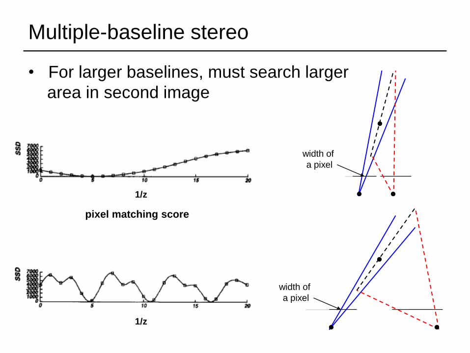
Multiple-baseline stereo
• For larger baselines, must search larger
area in second image
1/z
width of
a pixel
width of
a pixel
1/z
pixel matching score

Multiple-baseline stereo
Use the sum of
SSD scores to rank
matches
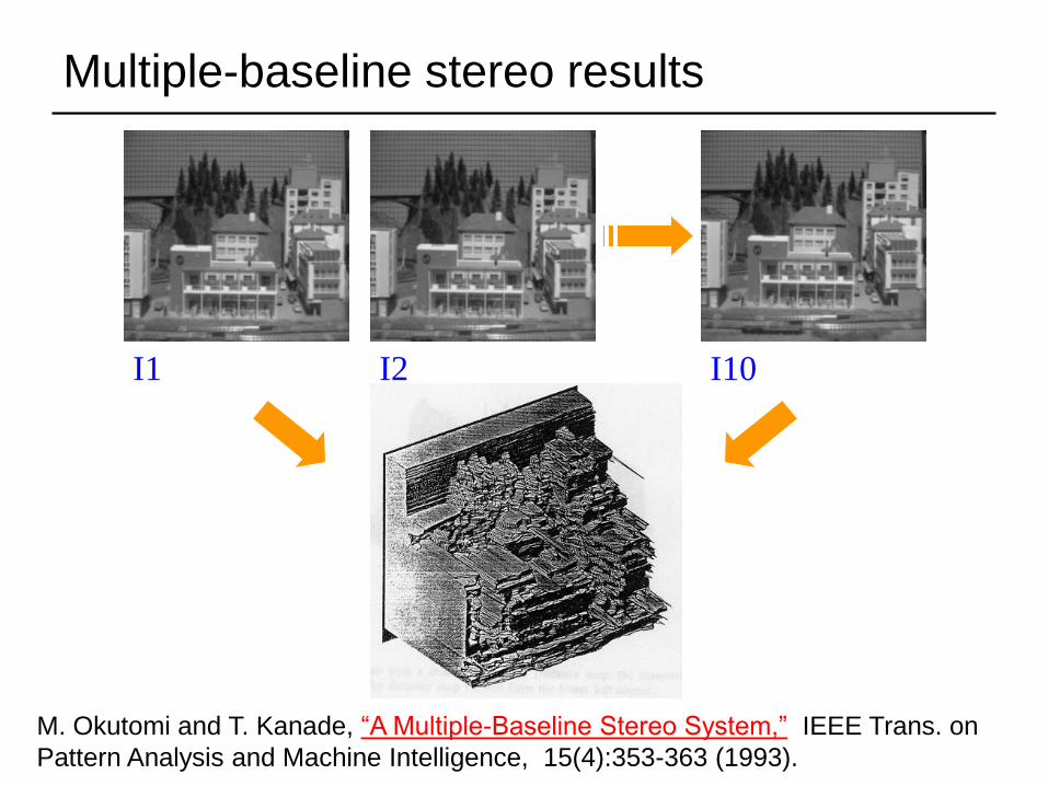
I1 I2 I10
Multiple-baseline stereo results
M. Okutomi and T. Kanade, “A Multiple-Baseline Stereo System,” IEEE Trans. on
Pattern Analysis and Machine Intelligence, 15(4):353-363 (1993).

Summary: Multiple-baseline stereo
• Pros
• Using multiple images reduces the ambiguity of matching
• Cons
• Must choose a reference view
• Occlusions become an issue for large baseline
• Possible solution: use a virtual view
Volumetric stereo
• In plane sweep stereo, the sampling of the scene
still depends on the reference view
• We can use a voxel volume to get a view-
independent representation

Volumetric Stereo / Voxel Coloring
Discretized
Scene Volume
Input Images
(Calibrated)
Goal: Assign RGB values to voxels in Vphoto-consistent with images
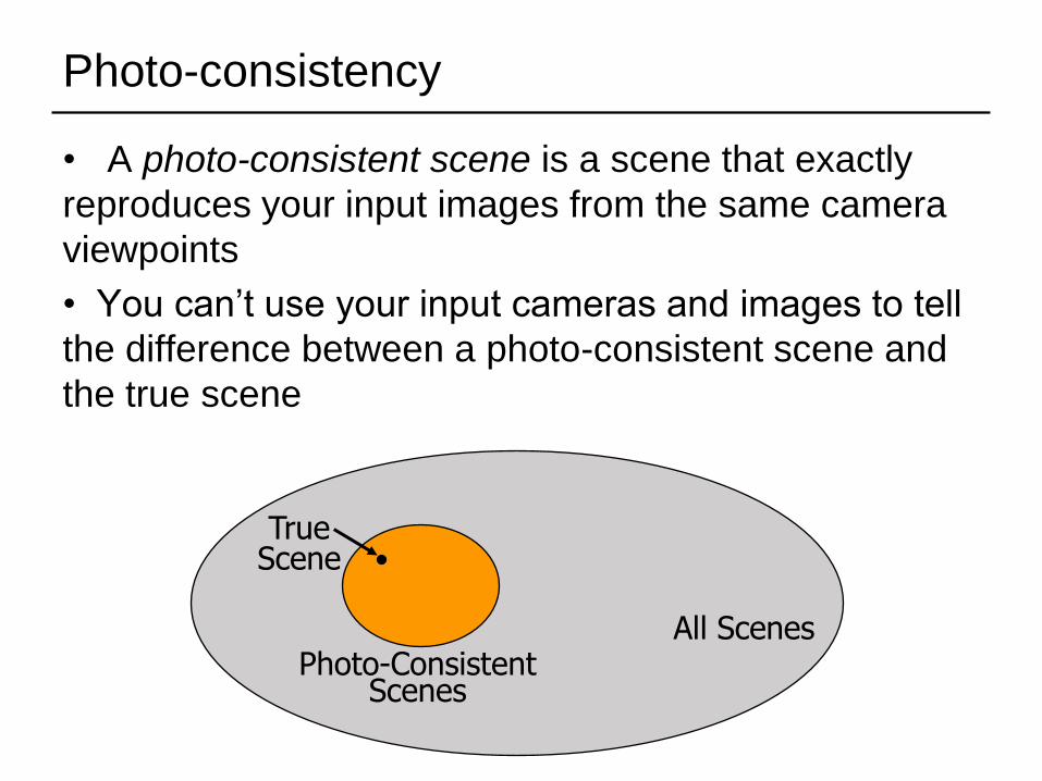
Photo-consistency
All ScenesPhoto-Consistent
Scenes
TrueScene
• A photo-consistent scene is a scene that exactly
reproduces your input images from the same camera
viewpoints
• You can’t use your input cameras and images to tell
the difference between a photo-consistent scene and
the true scene
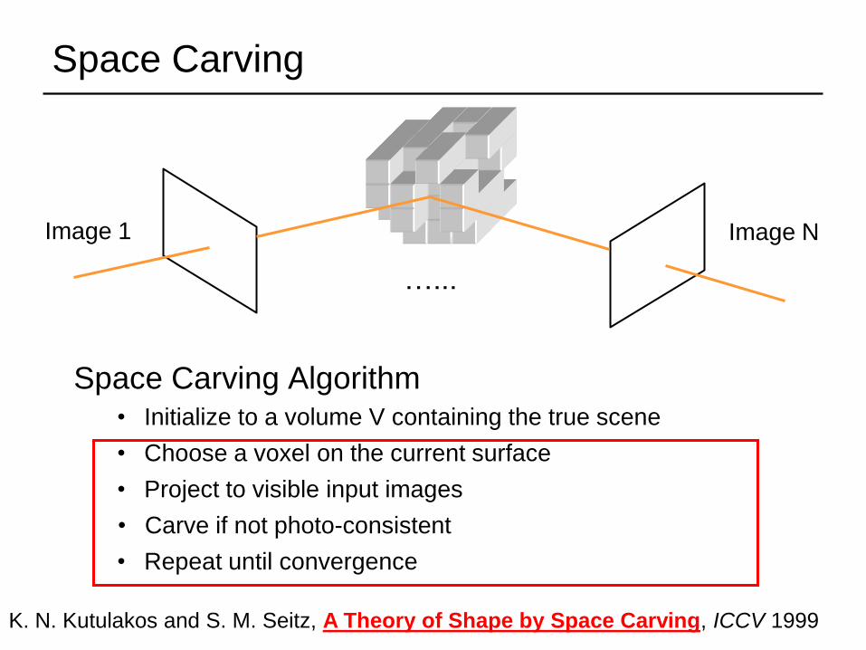
Space Carving
Space Carving Algorithm
Image 1 Image N
…...
• Initialize to a volume V containing the true scene
• Repeat until convergence
• Choose a voxel on the current surface
• Carve if not photo-consistent
• Project to visible input images
K. N. Kutulakos and S. M. Seitz, A Theory of Shape by Space Carving, ICCV 1999

Which shape do you get?
The Photo Hull is the UNION of all photo-consistent scenes in V
• It is a photo-consistent scene reconstruction
• Tightest possible bound on the true scene
True Scene
V
Photo Hull
V
Source: S. Seitz

Space Carving Results: African Violet
Input Image (1 of 45) Reconstruction
ReconstructionReconstruction Source: S. Seitz

Space Carving Results: Hand
Input Image(1 of 100)
Views of Reconstruction

Reconstruction from Silhouettes
Binary Images
• The case of binary images: a voxel is photo-
consistent if it lies inside the object’s silhouette in all
views

Reconstruction from Silhouettes
Binary Images
Finding the silhouette-consistent shape (visual hull):
• Backproject each silhouette
• Intersect backprojected volumes
• The case of binary images: a voxel is photo-
consistent if it lies inside the object’s silhouette in all
views

Volume intersection
Reconstruction Contains the True Scene
• But is generally not the same

Voxel algorithm for volume intersection
Color voxel black if on silhouette in every image

Photo-consistency vs. silhouette-consistency
True Scene Photo Hull Visual Hull

Carved visual hulls
• The visual hull is a good starting point for optimizing
photo-consistency
• Easy to compute
• Tight outer boundary of the object
• Parts of the visual hull (rims) already lie on the surface and are
already photo-consistent
Yasutaka Furukawa and Jean Ponce, Carved Visual Hulls for Image-Based
Modeling, ECCV 2006.

Carved visual hulls
1. Compute visual hull
2. Use dynamic programming to find rims and
constrain them to be fixed
3. Carve the visual hull to optimize photo-consistency
Yasutaka Furukawa and Jean Ponce, Carved Visual Hulls for Image-Based
Modeling, ECCV 2006.
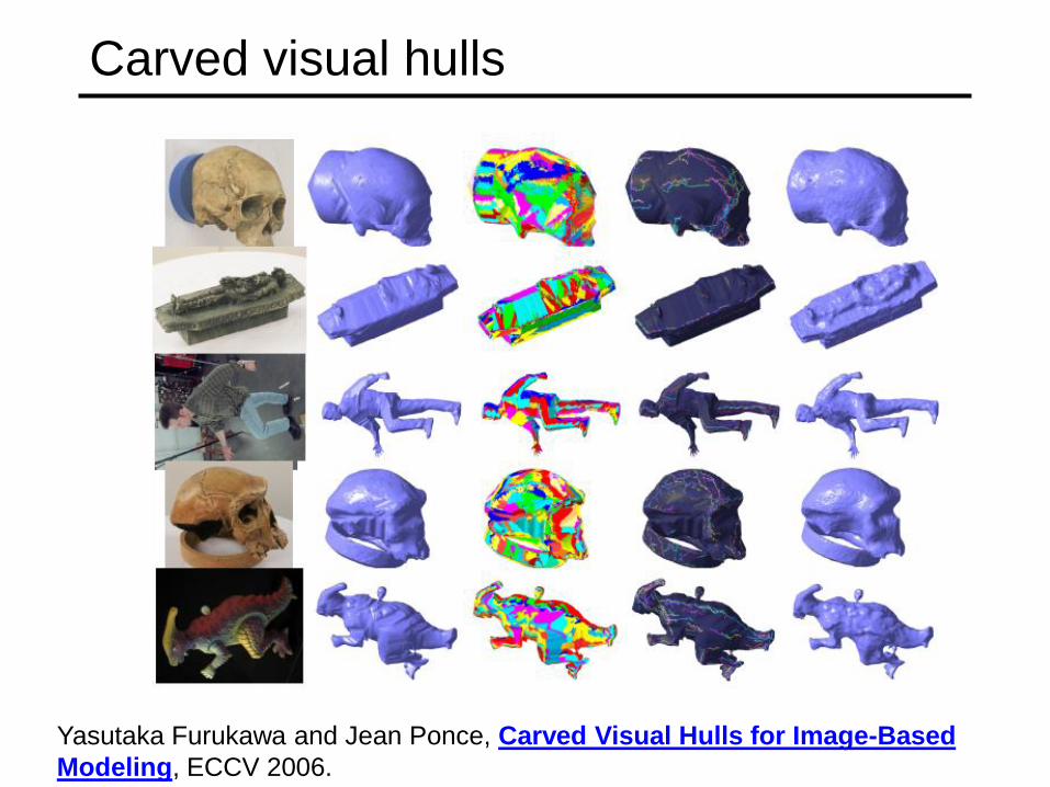
Carved visual hulls
Yasutaka Furukawa and Jean Ponce, Carved Visual Hulls for Image-Based
Modeling, ECCV 2006.

Carved visual hulls: Pros and cons
• Pros
• Visual hull gives a reasonable initial mesh that can be
iteratively deformed
• Cons
• Need silhouette extraction
• Have to compute a lot of points that don’t lie on the object
• Finding rims is difficult
• The carving step can get caught in local minima
• Possible solution: use sparse feature
correspondences as initialization

From feature matching to dense stereo
1. Extract features
2. Get a sparse set of initial matches
3. Iteratively expand matches to nearby locations
4. Use visibility constraints to filter out false matches
5. Perform surface reconstruction
Yasutaka Furukawa and Jean Ponce, Accurate, Dense, and Robust Multi-View
Stereopsis, CVPR 2007.

From feature matching to dense stereo
Yasutaka Furukawa and Jean Ponce, Accurate, Dense, and Robust Multi-View
Stereopsis, CVPR 2007.
http://www.cs.washington.edu/homes/furukawa/gallery/

Stereo from community photo collections
M. Goesele, N. Snavely, B. Curless, H. Hoppe, S. Seitz, Multi-View Stereo for
Community Photo Collections, ICCV 2007
http://grail.cs.washington.edu/projects/mvscpc/

Stereo from community photo collections
M. Goesele, N. Snavely, B. Curless, H. Hoppe, S. Seitz, Multi-View Stereo for
Community Photo Collections, ICCV 2007
stereo laser scan
Comparison: 90% of points
within 0.128 m of laser scan
(building height 51m)

Stereo from community photo collections
• Up to now, we’ve always assumed that camera
calibration is known
• For photos taken from the Internet, we need structure
from motion techniques to reconstruct both camera
positions and 3D points

Multi-view stereo: Summary
• Multiple-baseline stereo
• Pick one input view as reference
• Inverse depth instead of disparity
• Volumetric stereo
• Photo-consistency
• Space carving
• Shape from silhouettes
• Visual hull: intersection of visual cones
• Carved visual hulls
• Feature-based stereo
• From sparse to dense correspondences

Overview
Multi-view stereo
Structure from Motion (SfM)
Large scale Structure from Motion

Structure from motion

Multiple-view geometry questions
• Scene geometry (structure): Given 2D point matches in two or more images, where are the corresponding points in 3D?
• Correspondence (stereo matching): Given a point in just one image, how does it constrain the position of the corresponding point in another image?
• Camera geometry (motion): Given a set of corresponding points in two or more images, what are the camera matrices for these views?
Slide: S. Lazebnik

Structure from motion
• Given: m images of n fixed 3D points
xij = Pi Xj , i = 1, … , m, j = 1, … , n
• Problem: estimate m projection matrices Pi and
n 3D points Xj from the mn correspondences xij
x1j
x2j
x3j
Xj
P1
P2
P3
Slide: S. Lazebnik

Structure from motion ambiguity
• If we scale the entire scene by some factor k and, at
the same time, scale the camera matrices by the
factor of 1/k, the projections of the scene points in the
image remain exactly the same:
It is impossible to recover the absolute scale of the scene!
)(1
XPPXx kk
Slide: S. Lazebnik

Structure from motion ambiguity
• If we scale the entire scene by some factor k and, at
the same time, scale the camera matrices by the
factor of 1/k, the projections of the scene points in the
image remain exactly the same
• More generally: if we transform the scene using a
transformation Q and apply the inverse
transformation to the camera matrices, then the
images do not change
QXPQPXx-1
Slide: S. Lazebnik

Types of ambiguity
vTv
tAProjective
15dof
Affine
12dof
Similarity
7dof
Euclidean
6dof
Preserves intersection and
tangency
Preserves parallellism,
volume ratios
Preserves angles, ratios of
length
10
tAT
10
tRT
s
10
tRT
Preserves angles, lengths
• With no constraints on the camera calibration matrix or on the scene, we get a projective reconstruction
• Need additional information to upgrade the reconstruction to affine, similarity, or Euclidean
Slide: S. Lazebnik

Projective ambiguity
XQPQPXx P
-1
P

Projective ambiguity

Affine ambiguity
XQPQPXx A
-1
A
Affine

Affine ambiguity

Similarity ambiguity
XQPQPXx S
-1
S

Similarity ambiguity

Structure from motion
• Let’s start with affine cameras (the math is easier)
center at
infinity

Recall: Orthographic Projection
Special case of perspective projection
• Distance from center of projection to image plane is infinite
• Projection matrix:
Image World
Slide by Steve Seitz

Orthographic Projection
Parallel Projection
Affine cameras

Affine cameras
• A general affine camera combines the effects of an
affine transformation of the 3D space, orthographic
projection, and an affine transformation of the image:
• Affine projection is a linear mapping + translation in
inhomogeneous coordinates
10
bAP
1000
]affine44[
1000
0010
0001
]affine33[ 2232221
1131211
baaa
baaa
x
Xa1
a2
bAXx
2
1
232221
131211
b
b
Z
Y
X
aaa
aaa
y
x
Projection of
world origin

Affine structure from motion
• Given: m images of n fixed 3D points:
xij = Ai Xj + bi , i = 1,… , m, j = 1, … , n
• Problem: use the mn correspondences xij to estimate m projection matrices Ai and translation vectors bi, and n points Xj
• The reconstruction is defined up to an arbitrary affine transformation Q (12 degrees of freedom):
• We have 2mn knowns and 8m + 3n unknowns (minus 12 dof for affine ambiguity)
• Thus, we must have 2mn >= 8m + 3n – 12
• For two views, we need four point correspondences
1
XQ
1
X,Q
10
bA
10
bA1

Affine structure from motion
• Centering: subtract the centroid of the image points
• For simplicity, assume that the origin of the world
coordinate system is at the centroid of the 3D points
• After centering, each normalized point xij is related to
the 3D point Xi by
ji
n
k
kji
n
k
ikiiji
n
k
ikijij
n
nn
XAXXA
bXAbXAxxx
ˆ1
11ˆ
1
11
jiij XAx ˆ

Affine structure from motion
• Let’s create a 2m × n data (measurement) matrix:
mnmm
n
n
xxx
xxx
xxx
D
ˆˆˆ
ˆˆˆ
ˆˆˆ
21
22221
11211
cameras
(2m)
points (n)
C. Tomasi and T. Kanade. Shape and motion from image streams under orthography:
A factorization method. IJCV, 9(2):137-154, November 1992.

Affine structure from motion
• Let’s create a 2m × n data (measurement) matrix:
n
mmnmm
n
n
XXX
A
A
A
xxx
xxx
xxx
D
21
2
1
21
22221
11211
ˆˆˆ
ˆˆˆ
ˆˆˆ
cameras
(2m × 3)
points (3 × n)
The measurement matrix D = MS must have rank 3!
C. Tomasi and T. Kanade. Shape and motion from image streams under orthography:
A factorization method. IJCV, 9(2):137-154, November 1992.

Factorizing the measurement matrix
Source: M. Hebert

Factorizing the measurement matrix
• Singular value decomposition of D:
Source: M. Hebert

Factorizing the measurement matrix
• Singular value decomposition of D:
Source: M. Hebert

Factorizing the measurement matrix
• Obtaining a factorization from SVD:
Source: M. Hebert

Factorizing the measurement matrix
• Obtaining a factorization from SVD:
Source: M. Hebert
This decomposition minimizes
|D-MS|2

Affine ambiguity
• The decomposition is not unique. We get the same D
by using any 3×3 matrix C and applying the
transformations M → MC, S →C-1S
• That is because we have only an affine transformation
and we have not enforced any Euclidean constraints
(like forcing the image axes to be perpendicular, for
example)
Source: M. Hebert
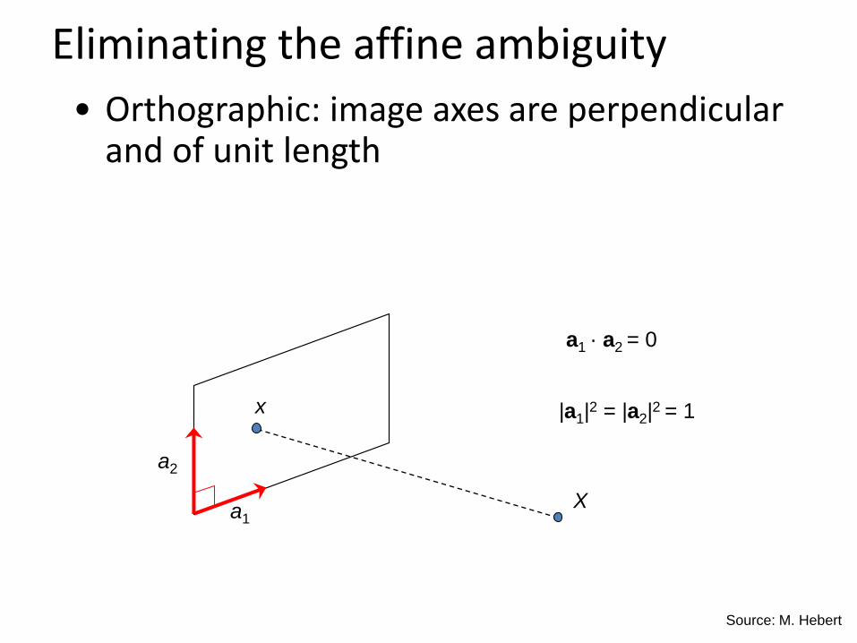
• Orthographic: image axes are perpendicular and of unit length
Eliminating the affine ambiguity
x
Xa1
a2
a1 · a2 = 0
|a1|2 = |a2|
2 = 1
Source: M. Hebert

Solve for orthographic constraints
• Solve for L = CCT
• Recover C from L by Cholesky decomposition: L = CCT
• Update A and X: A = AC, X = C-1X
T
i
T
i
i
2
1
~
~~
a
aAwhere
1~~11 T
i
TT
i aCCa
1~~22 T
i
TT
i aCCa
0~~21 T
i
TT
i aCCa
~ ~
Three equations for each image i
Slide: D. Hoiem

Algorithm summary
• Given: m images and n features xij
• For each image i, center the feature coordinates
• Construct a 2m × n measurement matrix D:
• Column j contains the projection of point j in all views
• Row i contains one coordinate of the projections of all the n
points in image i
• Factorize D:
• Compute SVD: D = U W VT
• Create U3 by taking the first 3 columns of U
• Create V3 by taking the first 3 columns of V
• Create W3 by taking the upper left 3 × 3 block of W
• Create the motion and shape matrices:
• M = U3W3½ and S = W3
½ V3T (or M = U3 and S = W3V3
T)
• Eliminate affine ambiguitySource: M. Hebert

Reconstruction results
C. Tomasi and T. Kanade. Shape and motion from image streams under orthography:
A factorization method. IJCV, 9(2):137-154, November 1992.

Dealing with missing data
• So far, we have assumed that all points are visible in
all views
• In reality, the measurement matrix typically looks
something like this:
cameras
points

Dealing with missing data
• Possible solution: decompose matrix into dense sub-
blocks, factorize each sub-block, and fuse the results
• Finding dense maximal sub-blocks of the matrix is NP-
complete (equivalent to finding maximal cliques in a graph)
• Incremental bilinear refinement
(1) Perform
factorization on a
dense sub-block
(2) Solve for a new
3D point visible by
at least two known
cameras (linear
least squares)
(3) Solve for a new
camera that sees at
least three known
3D points (linear
least squares)
F. Rothganger, S. Lazebnik, C. Schmid, and J. Ponce. Segmenting, Modeling, and
Matching Video Clips Containing Multiple Moving Objects. PAMI 2007.

Projective structure from motion
• Given: m images of n fixed 3D points
zij xij = Pi Xj , i = 1,… , m, j = 1, … , n
• Problem: estimate m projection matrices Pi and n 3D
points Xj from the mn correspondences xij
x1j
x2j
x3j
Xj
P1
P2
P3

Projective structure from motion
• Given: m images of n fixed 3D points
zij xij = Pi Xj , i = 1,… , m, j = 1, … , n
• Problem: estimate m projection matrices Pi and n 3D
points Xj from the mn correspondences xij
• With no calibration info, cameras and points can only
be recovered up to a 4x4 projective transformation Q:
X → QX, P → PQ-1
• We can solve for structure and motion when
2mn >= 11m +3n – 15
• For two cameras, at least 7 points are needed

Projective SFM: Two-camera case
• Compute fundamental matrix F between the two views
• First camera matrix: [I|0]
• Second camera matrix: [A|b]
• Then b is the epipole (FTb = 0), A = –[b×]F
F&P sec. 13.3.1
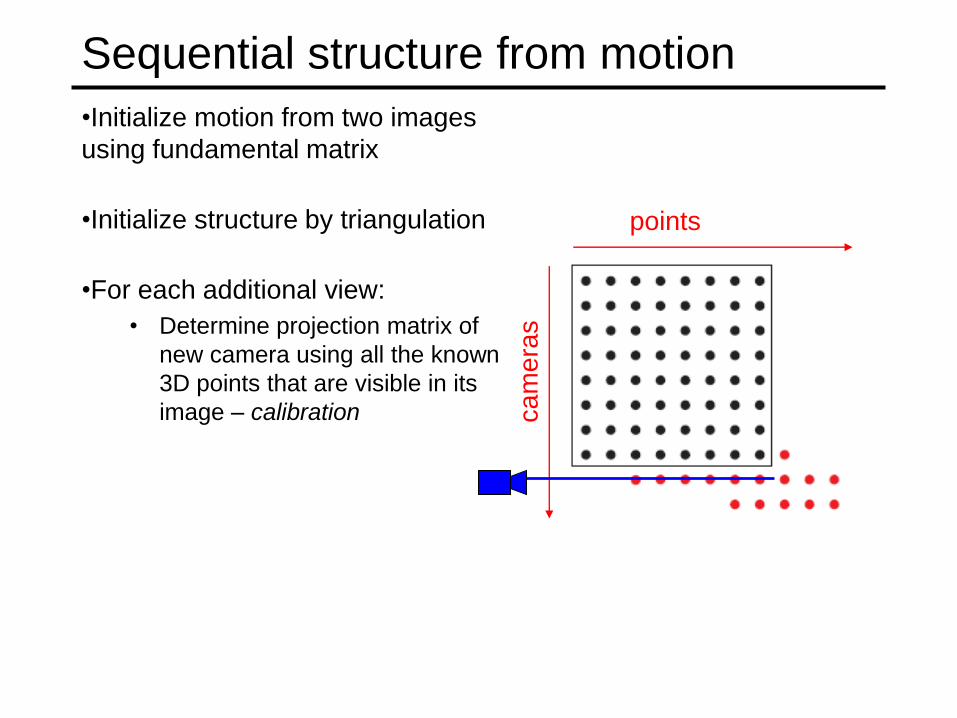
Sequential structure from motion
•Initialize motion from two images
using fundamental matrix
•Initialize structure by triangulation
•For each additional view:
• Determine projection matrix of
new camera using all the known
3D points that are visible in its
image – calibration ca
me
ras
points

Sequential structure from motion
•Initialize motion from two images
using fundamental matrix
•Initialize structure by triangulation
•For each additional view:
• Determine projection matrix of
new camera using all the known
3D points that are visible in its
image – calibration
• Refine and extend structure:
compute new 3D points,
re-optimize existing points that
are also seen by this camera –
triangulation
ca
me
ras
points

Sequential structure from motion
•Initialize motion from two images
using fundamental matrix
•Initialize structure by triangulation
•For each additional view:
• Determine projection matrix of
new camera using all the known
3D points that are visible in its
image – calibration
• Refine and extend structure:
compute new 3D points,
re-optimize existing points that
are also seen by this camera –
triangulation
•Refine structure and motion:
bundle adjustment
ca
me
ras
points

Bundle adjustment
• Non-linear method for refining structure and motion
• Minimizing reprojection error
2
1 1
,),(
m
i
n
j
jiijDE XPxXP
x1j
x2j
x3j
Xj
P1
P2
P3
P1Xj
P2Xj
P3Xj

Self-calibration
• Self-calibration (auto-calibration) is the process of
determining intrinsic camera parameters directly from
uncalibrated images
• For example, when the images are acquired by a
single moving camera, we can use the constraint that
the intrinsic parameter matrix remains fixed for all the
images
• Compute initial projective reconstruction and find 3D
projective transformation matrix Q such that all camera
matrices are in the form Pi = K [Ri | ti]
• Can use constraints on the form of the calibration
matrix: zero skew

Review: Structure from motion
• Ambiguity
• Affine structure from motion
• Factorization
• Dealing with missing data
• Incremental structure from motion
• Projective structure from motion
• Bundle adjustment
• Self-calibration
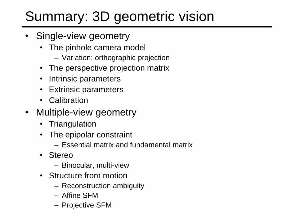
Summary: 3D geometric vision
• Single-view geometry• The pinhole camera model
– Variation: orthographic projection
• The perspective projection matrix
• Intrinsic parameters
• Extrinsic parameters
• Calibration
• Multiple-view geometry• Triangulation
• The epipolar constraint
– Essential matrix and fundamental matrix
• Stereo
– Binocular, multi-view
• Structure from motion
– Reconstruction ambiguity
– Affine SFM
– Projective SFM

Overview
Multi-view stereo
Structure from Motion (SfM)
Large scale Structure from Motion

Large-scale Structure from motion
Given many images from photo collections how can we
a) figure out where they were all taken from?
b) build a 3D model of the scene?
This is (roughly) the structure from motion problem
Slides from N. Snavely

Large-scale structure from motion
Dubrovnik, Croatia. 4,619 images (out of an initial 57,845).Total reconstruction time: 23 hoursNumber of cores: 352
Slide: N. Snavely

Structure from motion
• Input: images with points in correspondence pi,j = (ui,j,vi,j)
• Output• structure: 3D location xi for each point pi• motion: camera parameters Rj , tj possibly Kj
• Objective function: minimize reprojection error
Reconstruction (side)(top)

Photo Tourism
Slide: N. Snavely

First step: how to get correspondence?
Feature detection and matching

Feature detection
Detect features using SIFT [Lowe, IJCV 2004]

Feature detection
Detect features using SIFT [Lowe, IJCV 2004]

Feature matching
Match features between each pair of images

Feature matching
Refine matching using RANSAC to estimate fundamental
matrix between each pair

p1,1
p1,2p1,3
Image 1
Image 2
Image 3
x1
x4
x3
x2
x5
x6
x7
R1,t1
R2,t2
R3,t3
Slide: N. Snavely

Structure from motion
Camera 1
Camera 2
Camera 3
R1,t1
R2,t2
R3,t3
p1
p4
p3
p2
p5
p6
p7
minimize
f (R,T,P)
Slide: N. Snavely

Problem size
Trevi Fountain collection
466 input photos
+ > 100,000 3D points
= very large optimization problem

Incremental structure from motion

Incremental structure from motion
Slide: N. Snavely

Incremental structure from motion
Slide: N. Snavely
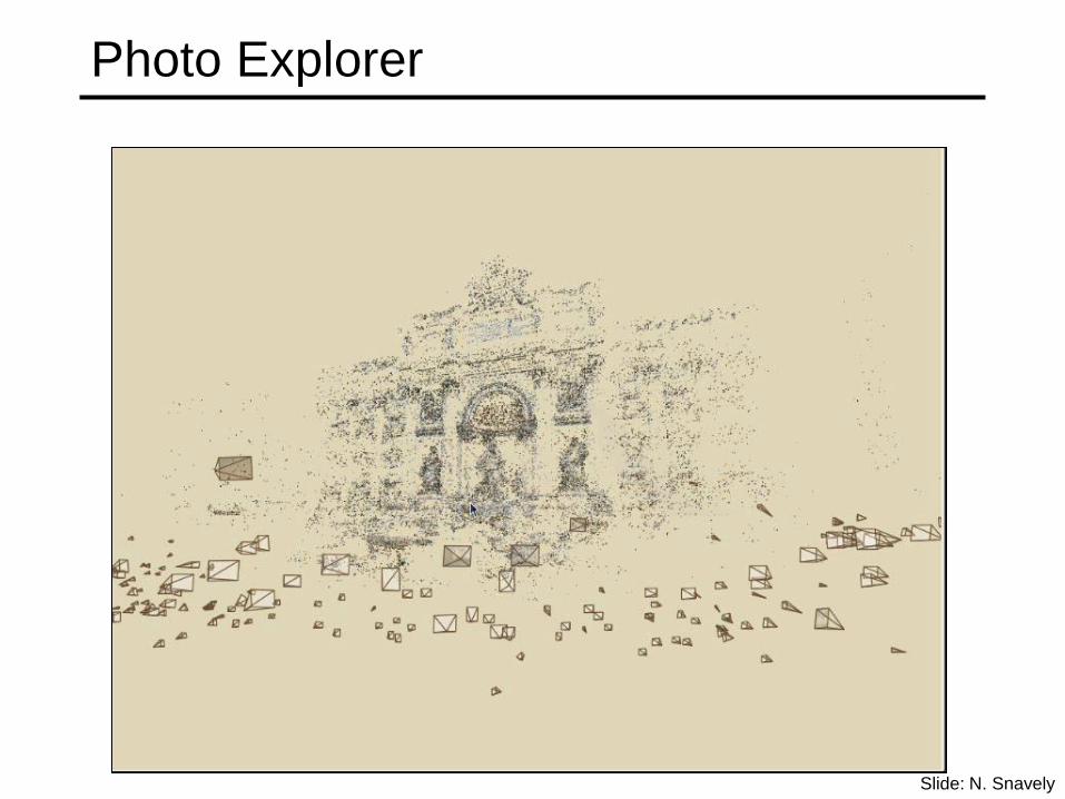
Photo Explorer
Slide: N. Snavely

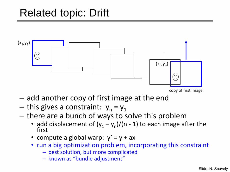
Related topic: Drift
copy of first image
(xn,yn)
(x1,y1)
– add another copy of first image at the end– this gives a constraint: yn = y1
– there are a bunch of ways to solve this problem• add displacement of (y1 – yn)/(n - 1) to each image after the
first• compute a global warp: y’ = y + ax• run a big optimization problem, incorporating this constraint
– best solution, but more complicated– known as “bundle adjustment”
Slide: N. Snavely
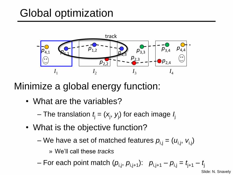
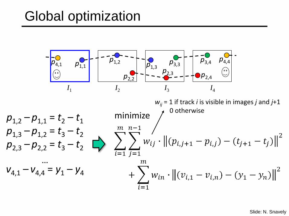
Global optimization
Minimize a global energy function:
• What are the variables?
– The translation tj = (xj, yj) for each image Ij
• What is the objective function?
– We have a set of matched features pi,j = (ui,j, vi,j)
» We’ll call these tracks
– For each point match (pi,j, pi,j+1): pi,j+1 – pi,j = tj+1 – tj
I1 I2 I3 I4
p1,1p1,2 p1,3
p2,2
p2,3 p2,4
p3,3p3,4 p4,4p4,1
track
Slide: N. Snavely
Global optimization
I1 I2 I3 I4
p1,1p1,2 p1,3
p2,2
p2,3 p2,4
p3,3p3,4 p4,4p4,1
p1,2 – p1,1 = t2 – t1
p1,3 – p1,2 = t3 – t2
p2,3 – p2,2 = t3 – t2
…v4,1 – v4,4 = y1 – y4
minimize
wij = 1 if track i is visible in images j and j+10 otherwise
Slide: N. Snavely

Global optimization
I1 I2 I3 I4
p1,1p1,2 p1,3
p2,2
p2,3 p2,4
p3,3p3,4 p4,4p4,1
A2m x 2n 2n x 1
x2m x 1
bSlide: N. Snavely

Global optimization
Defines a least squares problem: minimize
• Solution:
• Problem: there is no unique solution for ! (det = 0)
• We can add a global offset to a solution and get the same error
A2m x 2n 2n x 1
x2m x 1
b
Slide: N. Snavely

Ambiguity in global location
Each of these solutions has the same error
Called the gauge ambiguity
Solution: fix the position of one image (e.g., make the origin of the 1st image (0,0))
(0,0)
(-100,-100)
(200,-200)

Solving for camera rotation
Instead of spherically warping the images and solving
for translation, we can directly solve for the rotation Rj
of each camera
Can handle tilt / twist

Solving for rotations
R1
R2
f
I1
I2
p12 = (u12, v12)
p11 = (u11, v11)
(u11, v11, f) = p11
R1p11
R2p22

Solving for rotations
minimize

3D rotations
How many degrees of freedom are there?
How do we represent a rotation?
• Rotation matrix (too many degrees of freedom)
• Euler angles (e.g. yaw, pitch, and roll) – bad idea
• Quaternions (4-vector on unit sphere)
Usually involves non-linear optimization

p1,1
p1,2p1,3
Image 1
Image 2
Image 3
x1
x4
x3
x2
x5
x6
x7
R1,t1
R2,t2
R3,t3

SfM objective function
Given point x and rotation and translation R, t
Minimize sum of squared reprojection errors:
predictedimage location
observedimage location

Solving structure from motion
Minimizing g is difficult• g is non-linear due to rotations, perspective division• lots of parameters: 3 for each 3D point, 6 for each
camera• difficult to initialize• gauge ambiguity: error is invariant to a similarity
transform (translation, rotation, uniform scale)
Many techniques use non-linear least-squares (NLLS) optimization (bundle adjustment)• Levenberg-Marquardt is one common algorithm for
NLLS• Lourakis, The Design and Implementation of a
Generic Sparse Bundle Adjustment Software Package Based on the Levenberg-Marquardt Algorithm, http://www.ics.forth.gr/~lourakis/sba/
• http://en.wikipedia.org/wiki/Levenberg-Marquardt_algorithm

Extensions to SfM
Can also solve for intrinsic parameters (focal length, radial distortion, etc.)
Can use a more robust function than squared error, to avoid fitting to outliers
For more information, see: Triggs, et al, “Bundle Adjustment – A Modern Synthesis”, Vision Algorithms 2000.


![LAMP: 3D layered, adaptive-resolution, and multi ...zhu/CVIU_LAMP/article.pdf · 40 vision algorithms, such as in multi-view stereo [17,18] or general motion analysis 41 [10,11,22,23]](https://img.dokumen.tips/doc/110x75/5fae6aa90a16b63ad6022bad/lamp-3d-layered-adaptive-resolution-and-multi-zhucviulamp-40-vision.jpg)