Lecture 6:molecular geometry optimization

energy minima, transition states, simplex, steepest descent, conjugate gradients, Newton, quasi-Newton, BFGS, TRM, RFO

“My dear fellow, who will let you?”“That's not the point. The point is, who will stop me?”

Ayn Rand

Dr Ilya Kuprov, University of Southampton, 2012

(for all lecture notes and video records see http://spindynamics.org)

Molecular geometry optimizationWithin the Born-Oppenheimer approximation, the geometry of a molecule at zeroabsolute temperature corresponds to the minimum of the total energy:

0, ,

ˆ, , arg mini i i

i i i Tx y z

x y z H

The process of finding the coordinates that minimize the energy is known in thetrade as geometry optimization. It is usually the first step in the calculation.

If the gradient is zero and

All H eigenvalues positive => MinimumAll H eigenvalues negative => MaximumH eigenvalues of both signs => Saddle (transition state)

2

; ijii i j

E EE Hx x x

We usually look for zero gradient (a gradient is the steepestascent direction), but not all such points are minima:

J.B. Foresman, A. Frisch, Exploring Chemistry with Electronic Structure Methods, Gaussian, 1996.

Minimization methods: simplexNelder-Mead simplex method performs minimization by polygon node reflection,accompanied by expansion, contraction and line search where necessary.

Pro Contra

Does not require gradient information

Very slow – thousands of iterations even with simple

problems.

Works for discontinuous, noisy and irreproducible functions.

Often gets stuck on ridgesand in troughs.

Can jump out of a local minimum. No guarantee of convergence.

Simplex and other non-gradient methods are onlyused in desperate caseswhen gradient informationis not available and whenthe function is very noisyor discontinuous.

J.A. Nelder and R. Mead, Computer Journal, 1965 (7) 308-313.

Minimization methods: gradient descent

Characteristic zig-zagging pattern producedby the basic gradient descent method.

The basic gradient descent method repeatedly takes afixed step in the direction opposite to the direction ofthe local gradient of the objective function:

Pro Contra

Convergence is guaranteed. Becomes slow close to the minimum.

Easy to implement and understand. Not applicable to noisy functions

Relatively inexpensive. Always converges to the nearest local minimum.

1n n n nx x k f x

Rastrigin’sfunction

The step size may be adjusted at each iteration usingthe line search procedure:

arg minn n nk

k f x k f x

J.A. Snyman, Practical Mathematical Optimization, Springer, 2005.

Minimization methods: conjugate gradients

Fletcher-Reeves method:

Conjugate gradients method makes use of the gradienthistory to decide a better direction for the next step:

1 1 n n n n n n n nx x k h h f x h

2

21

nn

n

f x

f x

T1

21

n n nn

n

f x f x f x

f x

Polak-Ribiere method:

Gradient descent: 63 evaluations.

Conjugate gradients: 22 evaluations.

CG method does not exhibit the zig-zagging behaviour during conver-gence, but still tends to be quiteslow in very non-linear cases.CG is very useful for solving linearsystems of equations, but has beensuperseded by more sophisticatedquadratic step control methods fornon-linear optimization.

J.A. Snyman, Practical Mathematical Optimization, Springer, 2005.

Minimization methods: Newton-Raphson methodNewton-Raphson method approximates the objectivefunction by a quadratic surface at each step and movesto the minimum of that surface:

Pro Contra

Very fast convergence. Very expensive.

Well adapted for molecular geometry optimization. Not applicable to noisy functions.

Useful if Hessians are cheap(e.g. in molecular dynamics).

Always converges to the nearest local stationary point.

T T

1

1( ) ( )2

( )

( )

f x x f x f x x x x

f x x f x x

x f x

H

H

H

Newton-Raphson: 6 evaluations.

Gradient descent: 63 evaluations.

Variations of Newton-Raphson method are currentlythe primary geometry optimization algorithms in QCsoftware packages.

J. Nocedal, S.J. Wright, Numerical Optimization, Springer, 2006.

Minimization methods: quasi-Newton methodsThe most expensive part of Newton-Raphson method isthe Hessian. It turns out that a good approximateHessian may be extracted from the gradient history:

Newton-Raphson: 6 evaluations.

BFGS quasi-Newton: 13 evaluations.

1

1

1 1

( )

,

T T Tk k k k k k

k kT T Tk k k k k k

T Tk k k k k k

k k T Tk k k k k

k k k k k k

g s s g g gE Eg s g s g s

g g s sg s s s

g f x f x s x x

H

H HHH

H

H

DFP update(Davidon-Fletcher-Powell)

BFGS update(Broyden-Fletcher-Goldfarb-Shanno)

The BFGS method is particularly good. Quasi-Newtonmethods provide super-linear convergence at effectivelythe cost of the gradient descent method.

Initial estimates for the Hessian are often computedusing inexpensive methods, such as molecular mecha-nics or semi-empirics (this is what the connectivitydata is for in Gaussian).

J. Nocedal, S.J. Wright, Numerical Optimization, Springer, 2006.

Minimization methods: TRM and RFOThe basic Newton-Raphson method requires the Hessian to be non-singular andtends to develop problems if any of its eigenvalues become negative. A simple fixfor this is to add a regularization matrix (often a unit matrix):

1 ( )x f x H S

The two ways of doing this are known as trust region method and rational functionoptimization method. Both are implemented in Gaussian09. For TRM we have:

max 0, min eig H

and the step is scaled to stay within the trust radius. Rational functionoptimization introduces a step size dependent denominator, which prevents thealgorithm from taking large steps:

T T

T

1( )2( )

1

f x x x xf x x f x

x x

H

S

RFO behaves better than Newton-Raphson in the vicinity of inflection points.

R.H. Byrd, J.C. Gilbert, J. Nocedal, http://dx.doi.org/10.1007/PL00011391

Update the geometry

Update the Hessian(BFGS, DFP, etc.)

Geometry optimization flowchart

Initial guess for geometry and Hessian

Calculate energy and gradient

Minimize along the gradient direction line

Take a quadratic step(Newton, BFGS, TRM, RFO, etc.)

Check for convergence on the gradient and displacement

“yes” DONE

Take the step alongthe gradient.

“no”“no”

J.B. Foresman, A. Frisch, Exploring Chemistry with Electronic Structure Methods, Gaussian, 1996.

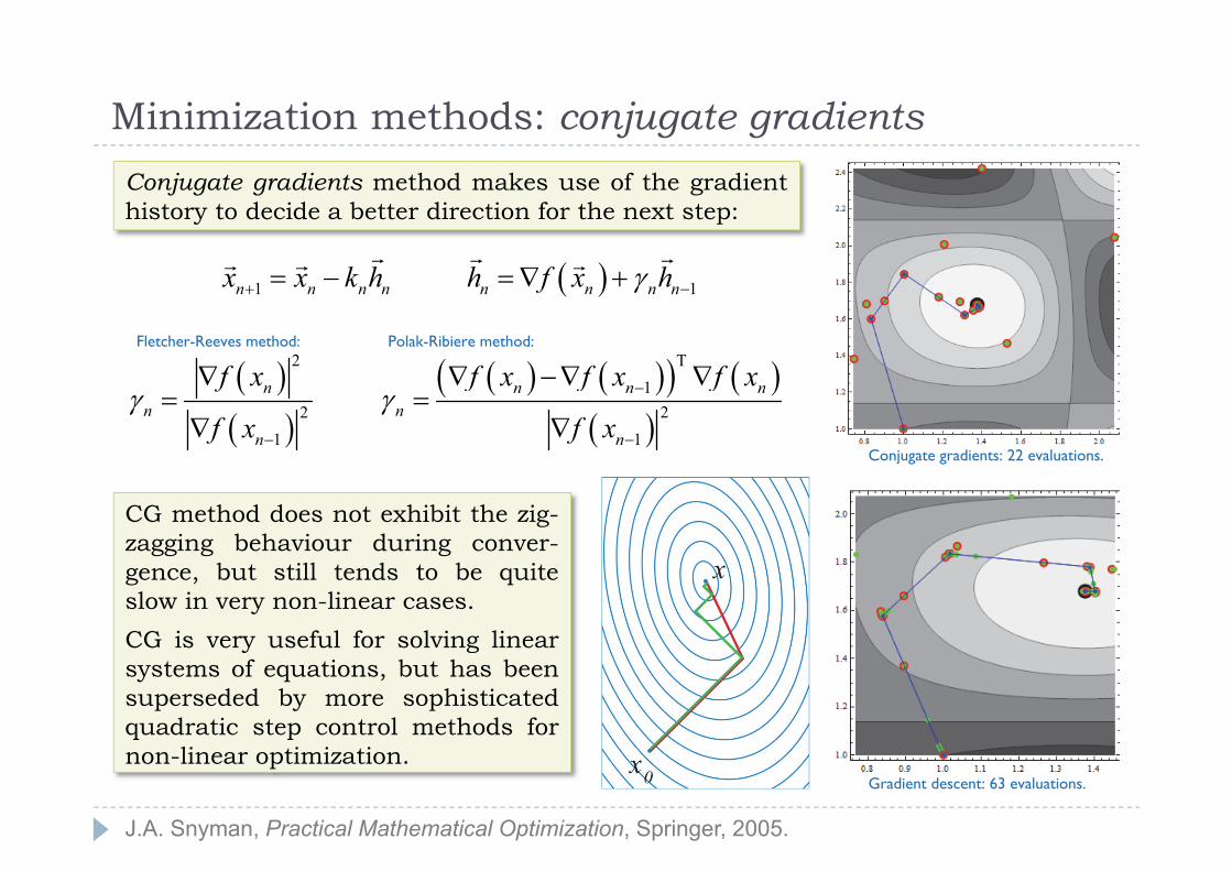
Intrinsic reaction coordinateIRC is defined as the minimum-energy reaction path on a potential energy surface inmass-weighted coordinates, connecting reactants to products.

1

0

IRC 0s

s

x s E x s dsx s

Because the reactants and the products are energy minima, the IRC path necessarilypasses through a saddle point, known as the transition state. Finding the transitionstate without system-specific knowledge is quite difficult (minima are usually easy).

An example of a complicated branching reactionpath (lanthanide complex isomerization).

F. Jensen, Introduction to Computational Chemistry, Wiley, 2007.

Coordinate driving and hypersphere searchCoordinate driving is also known as relaxed potential ener-gy scan. A particular internal coordinate (or a linear combi-nation thereof) is systematically scanned and the structureis optimized to a minimum with respect to other coordina-tes at each step.

Hypersphere search proceeds by locating all ener-gy minima on a hypersphere of a given radius inthe coordinate space and tracing these minima asa function of the sphere radius.Very expensive, but has the advantage of mappingall reaction paths from the given structure.

C. Peng, P.Y. Ayala, H.B. Schlegel, M.J. Frisch, J. Comp. Chem. 17 (1996) 49-56.

Newton and quasi-Newton methodsThe type of stationary point reached by quadratic algo-rithms depends on the definiteness of the Hessian. Inthe Hessian eigenframe we have:

If any eigenvalue is negative, the step would be performed not down, but up the gradientand the corresponding coordinate would be optimized into a maximum. Importantly, forindefinite Hessians the BFGS quasi-Newton update scheme becomes ill-conditioned. Itis commonly replaced by Bofill update scheme, which avoids that problem:

1 11 1

2 22 2

0 00 0

0 0N NN N

x H fx H f

x H f

TBOF SR1 PSB SR1

T

2T TT T TPSB

2 2 2T T

1 ,

,

g x g xg x x

x g xg x x x g x x g x x xx x x g xx x

H HH H H H

H

HH H HH

H

K.P. Lawley, H.B. Schlegel, http://dx.doi.org/10.1002/9780470142936.ch4

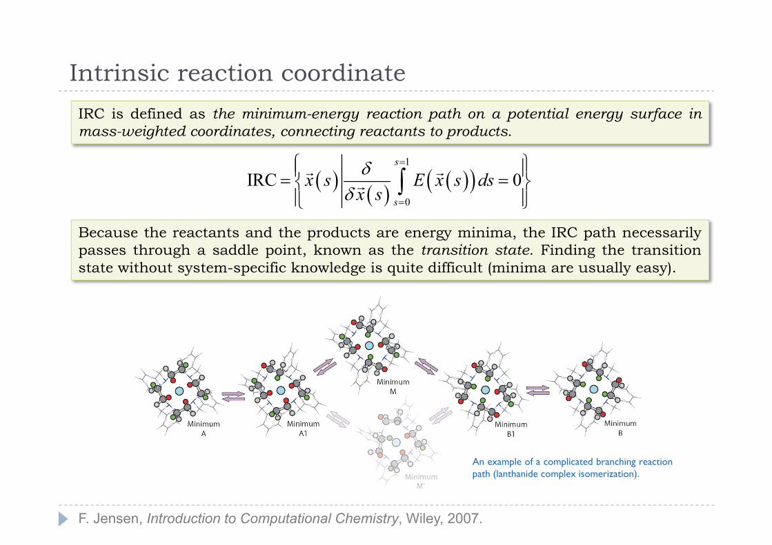
Eigenvector following methodIn principle, one could follow a particular normal modeout of the minimum and into a maximum by delibe-rately stepping uphill on that mode:1. Start at the minimum, compute and diagonalize the

Hessian matrix.2. Move in the direction of eigenvector of interest by a

user-specified initial step.3. Compute the gradient and the Hessian at the new

point. Diagonalize the Hessian.4. Take Newton steps in all directions except the

direction of the smallest eigenvalue. Take an uphillstep in that direction.

5. Repeat 2-4 until converged.

Advantages: very robust. Guarantees convergence intosome saddle point. Good choice for small systems.Downside: very expensive (a Hessian is computed ateach step). No guarantee that the saddle point is theone wanted. Rarely a good choice for systems with 50+coordinates.

A. Banerjee, N. Adams, J. Simons, R. Shepard, J. Phys. Chem. 89 (1985) 52-57.

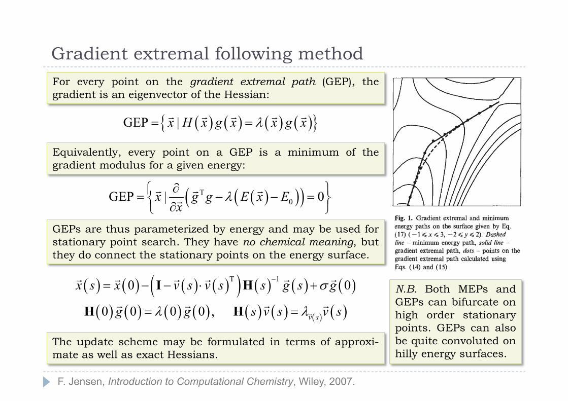
Gradient extremal following methodFor every point on the gradient extremal path (GEP), thegradient is an eigenvector of the Hessian:

Equivalently, every point on a GEP is a minimum of thegradient modulus for a given energy:

GEP |x H x g x x g x

GEPs are thus parameterized by energy and may be used forstationary point search. They have no chemical meaning, butthey do connect the stationary points on the energy surface.

T0GEP | 0x g g E x E

x

T 10 0

0 0 0 0 , v s

x s x v s v s s g s g

g g s v s v s

I H

H H

The update scheme may be formulated in terms of approxi-mate as well as exact Hessians.

N.B. Both MEPs andGEPs can bifurcate onhigh order stationarypoints. GEPs can alsobe quite convoluted onhilly energy surfaces.

F. Jensen, Introduction to Computational Chemistry, Wiley, 2007.

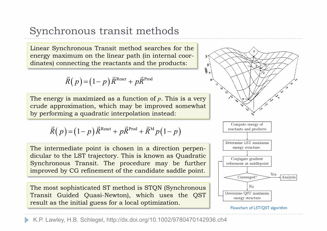
Synchronous transit methods

Flowchart of LST/QST algorithm

Linear Synchronous Transit method searches for theenergy maximum on the linear path (in internal coor-dinates) connecting the reactants and the products:

React Prod1R p p R pR

The energy is maximized as a function of p. This is a verycrude approximation, which may be improved somewhatby performing a quadratic interpolation instead:

React Prod M1 1R p p R pR R p p

The intermediate point is chosen in a direction perpen-dicular to the LST trajectory. This is known as QuadraticSynchronous Transit. The procedure may be furtherimproved by CG refinement of the candidate saddle point.

The most sophisticated ST method is STQN (SynchronousTransit Guided Quasi-Newton), which uses the QSTresult as the initial guess for a local optimization.

K.P. Lawley, H.B. Schlegel, http://dx.doi.org/10.1002/9780470142936.ch4

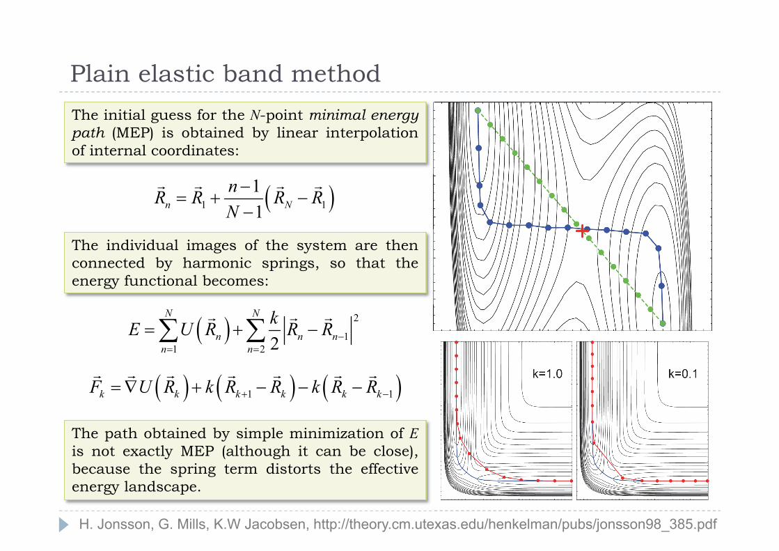
Plain elastic band methodThe initial guess for the N-point minimal energypath (MEP) is obtained by linear interpolationof internal coordinates:

1 111n N

nR R R RN

The individual images of the system are thenconnected by harmonic springs, so that theenergy functional becomes:

2

11 2 2

N N

n n nn n

kE U R R R

The path obtained by simple minimization of Eis not exactly MEP (although it can be close),because the spring term distorts the effectiveenergy landscape.

1 1k k k k k kF U R k R R k R R

H. Jonsson, G. Mills, K.W Jacobsen, http://theory.cm.utexas.edu/henkelman/pubs/jonsson98_385.pdf

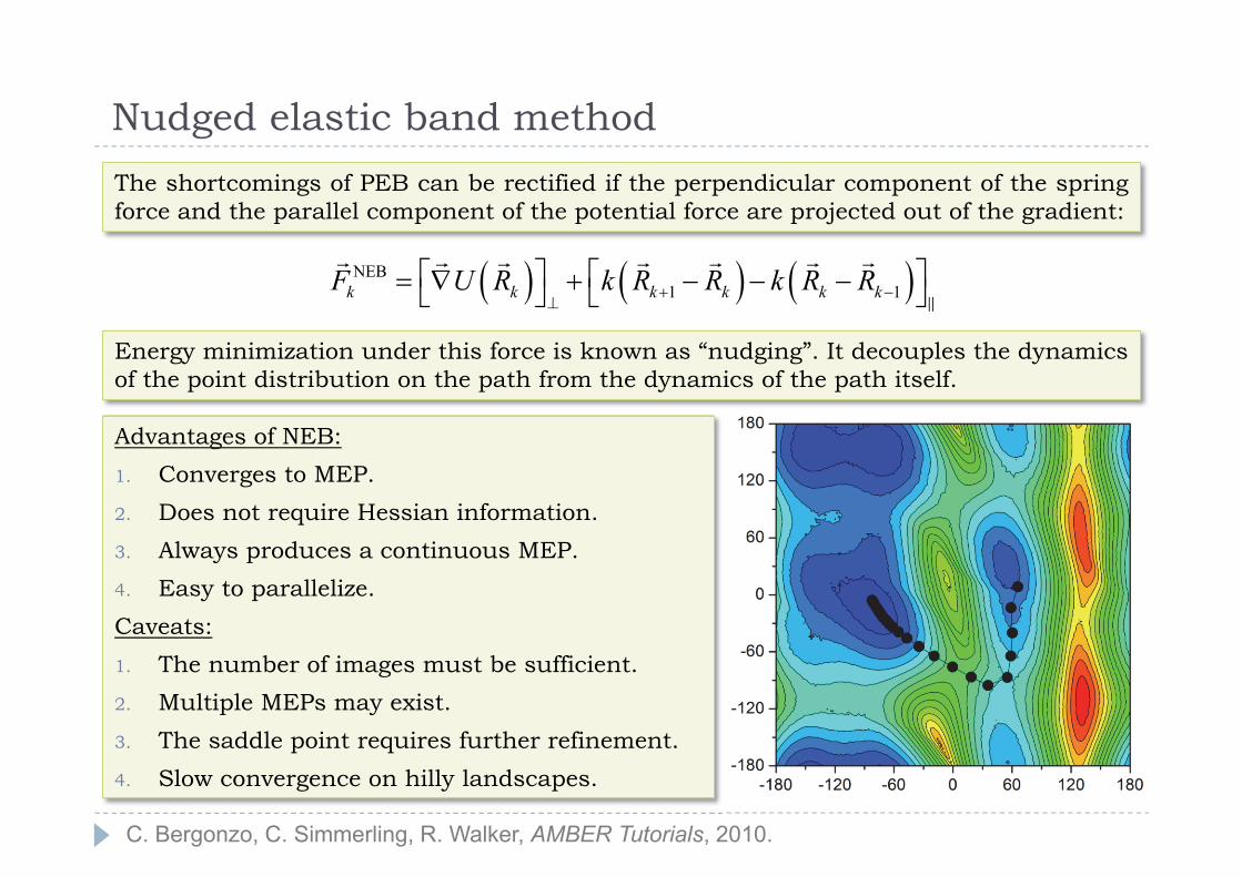
Nudged elastic band methodThe shortcomings of PEB can be rectified if the perpendicular component of the springforce and the parallel component of the potential force are projected out of the gradient:

Energy minimization under this force is known as “nudging”. It decouples the dynamicsof the point distribution on the path from the dynamics of the path itself.

NEB1 1k k k k k kF U R k R R k R R

Advantages of NEB:1. Converges to MEP.2. Does not require Hessian information.3. Always produces a continuous MEP.4. Easy to parallelize.Caveats:1. The number of images must be sufficient.2. Multiple MEPs may exist.3. The saddle point requires further refinement.4. Slow convergence on hilly landscapes.

C. Bergonzo, C. Simmerling, R. Walker, AMBER Tutorials, 2010.

Practical considerationsTransition states often have highly correlatedmulti-reference wavefunctions. Even CCSD(T)results would in many cases be an estimate.DFT calculations are often wrong by 20-50%.

R.J. Meier, E. Koglin, http://dx.doi.org/10.1016/S0009-2614(02)00032-5

Practical considerations

1. Gradient extremal following gets the stationary points, but not the reaction paths.2. Electrostatic environment can significantly alter the intermediate energy

(intermediates are often charged or have a large dipole moment).3. Convergence of saddle optimization is often slow – stock up on patience and tighten

up all tolerances.

H.B. Schlegel, J. Comp. Chem. 24 (2003) 1514-1527.

Practical considerations

If the Hessian has more than one negative eigenvalue, that is most probably not thestationary point you are looking for.

J.B. Foresman, A. Frisch, Exploring Chemistry with Electronic Structure Methods, Gaussian, 1996.

Practical considerations1. All gradient methods preserve molecular symmetry. It is your responsibility to

check for non-symmetric (e.g. due to Jahn-Teller effect) minima.2. Correctly chosen internal coordinates will significantly accelerate convergence.

Cartesian coordinates are almost always a bad choice.3. In multi-level optimizations, it is reasonable to retain the approximate Hessian

and use it as a guess for the higher level method.

H.B. Schlegel, Intl. J. Quant. Chem. 26 (1992) 243-252.

Miscellaneous notes1. Geometry optimization jobs should use tight convergence cut-offs at the SCF

stage to avoid numerical noise in the gradients.2. Invalid dihedrals (they appear in flat rings and linear systems) should be

avoided – any optimization in such systems is best performed in Cartesians.3. In very extended systems (e.g. carotene chains) small displacements of internal

coordinates can translate to large displacements in Cartesians. Convergencecriteria must be set appropriately.

4. The initial optimization of van der Waals complexes is best performed inCartesian coordinates.

5. If a very good approximation to a minimum is known, it is best to start awayfrom it – many numerical optimization algorithms crash if they cannot makethe initial step.

6. Positive definiteness must be strictly enforced in the Hessian when looking forenergy minima. Quasi-Newton optimizations with indefinite Hessians convergeinto saddle points.

7. Optimizations involving implicit solvent would not usually converge to thesame accuracy as vacuum calculations due to the numerical noise arising fromthe discretization of the solvent cavity.

J.B. Foresman, A. Frisch, Exploring Chemistry with Electronic Structure Methods, Gaussian, 1996.