Embed Size (px)
Citation preview

2/15/2016 1 1Lecture #6 – Fall 2015 1D. Mohr
151-0735: Dynamic behavior of materials and structures
by Borja Erice and Dirk Mohr
ETH Zurich, Department of Mechanical and Process Engineering,
Chair of Computational Modeling of Materials in Manufacturing
Lecture #6: • 3D Rate-independent Plasticity (cont.)
• Pressure-dependent plasticity
© 2015

2/15/2016 2 2Lecture #6 – Fall 2015 2D. Mohr
151-0735: Dynamic behavior of materials and structures
Three-dimensional Rate-independent Plasticity

2/15/2016 3 3Lecture #6 – Fall 2015 3D. Mohr
151-0735: Dynamic behavior of materials and structures
Additive strain rate decomposition
The strain rate is decomposed into an elastic and a plastic part,
pe εεε
The corresponding algorithmic decomposition of the strain increment associated wit finite time increments Dt reads
pe εεΔVε DDD )ln(
The above decomposition is an approximation of the well-established multiplicative decomposition of the total deformation gradient,
peFFF
The approximation (*) of (**) yields reasonable results in finite strain problems when the elastic strains are small compared to unity.
(*)
(**)

2/15/2016 4 4Lecture #6 – Fall 2015 4D. Mohr
151-0735: Dynamic behavior of materials and structures
Elastic constitutive equation
The linear elastic isotropic constitutive equation reads
eεCσ :
with C denoting the fourth-order elastic stiffness tensor. For notational convenience, the above stress-strain relationship is rewritten in vector notation
e
e
e
e
e
e
E
23
13
12
33
22
11
23
13
12
33
22
11
21
021
0021
0001
0001
0001
)21)(1(
with the Young’s modulus E and the Poisson’s ratio n.
Sym.
2/15/2016 5 5Lecture #6 – Fall 2015 5D. Mohr
151-0735: Dynamic behavior of materials and structures
Equivalent stress definition
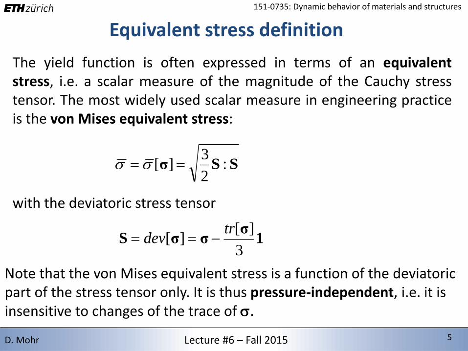
The yield function is often expressed in terms of an equivalentstress, i.e. a scalar measure of the magnitude of the Cauchy stresstensor. The most widely used scalar measure in engineering practiceis the von Mises equivalent stress:
SSσ :2
3][
with the deviatoric stress tensor
1σ
σσS3
][][
trdev
Note that the von Mises equivalent stress is a function of the deviatoricpart of the stress tensor only. It is thus pressure-independent, i.e. it is insensitive to changes of the trace of .

2/15/2016 6 6Lecture #6 – Fall 2015 6D. Mohr
151-0735: Dynamic behavior of materials and structures
Equivalent stress definition
The von Mises equivalent stress is an isotropic function, i.e. it isinvariant to rotations of the Cauchy stress tensor:
] [][ TRσRσ for any rotation
})()(){( 222
21
IIIIIIIIIIII
R
As an alternative it may also be expressed as a function of the stresstensor invariants or the principal stresses, e.g.
23J SS :21
2 Jwith
Von Mises plasticity models are therefore also often called J2-plasticity models.

2/15/2016 7 7Lecture #6 – Fall 2015 7D. Mohr
151-0735: Dynamic behavior of materials and structures
Yield function and surface
With the von Mises equivalent stress definition at hand, the yieldfunction is written as:
][][],[ pp kf σσ
I
II
III
The yield surface is
0],[ pf σ
2/15/2016 8 8Lecture #6 – Fall 2015 8D. Mohr
151-0735: Dynamic behavior of materials and structures
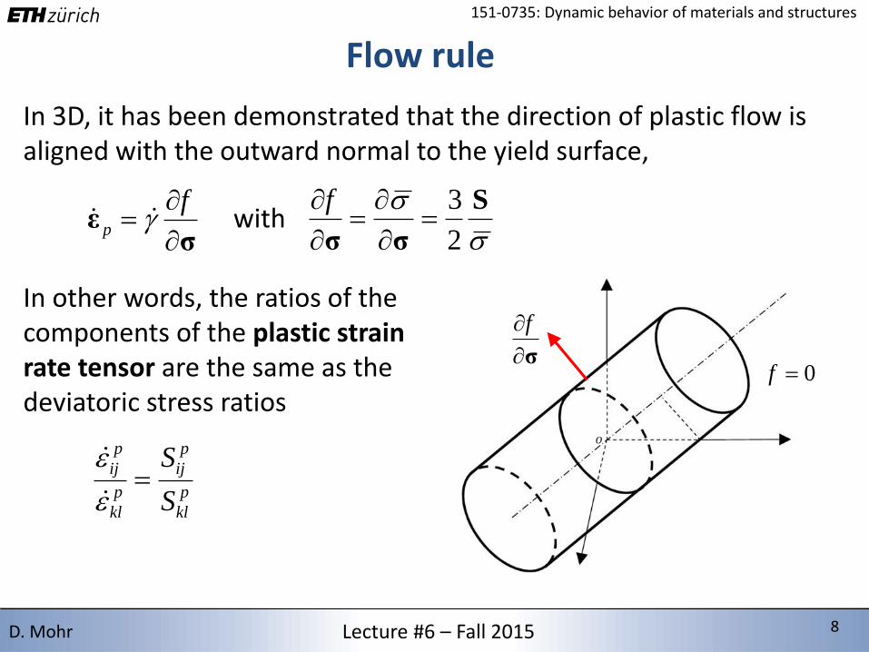
Flow rule
In 3D, it has been demonstrated that the direction of plastic flow is aligned with the outward normal to the yield surface,
σε
fp with
S
σσ 2
3
f
σ
f
0f
In other words, the ratios of the components of the plastic strain rate tensor are the same as the deviatoric stress ratios
p
kl
p
ij
p
kl
p
ij
S
S

2/15/2016 9 9Lecture #6 – Fall 2015 9D. Mohr
151-0735: Dynamic behavior of materials and structures
Flow rule
The proposed associated flow rule also implies that the plastic flow is incompressible (no volume change),
0][
2
3][
Sε
trtr p
σ
f
0f
The magnitude of the plastic strain rate tensor is controlled by the non-negative plastic multiplier . It is also called equivalent plastic strain rate.
0

2/15/2016 10 10Lecture #6 – Fall 2015 10D. Mohr
151-0735: Dynamic behavior of materials and structures
Isotropic strain hardening
The flow stress is expressed as a function of the equivalent plastic strain,
][ pkk ][
32
pk with
dttp ][
It controls the size of the elastic domain (diameter of the von Mises cylinder in stress space).

2/15/2016 11 11Lecture #6 – Fall 2015 11D. Mohr
151-0735: Dynamic behavior of materials and structures
Isotropic hardening
The same parametric forms for are used in 3D as in 1D.
n
pS Ak )( 0
][ pkk
]exp[10 pV Qkk
0.00E+00
5.00E+01
1.00E+02
1.50E+02
2.00E+02
2.50E+02
3.00E+02
3.50E+02
4.00E+02
0.00E+00
5.00E+01
1.00E+02
1.50E+02
2.00E+02
2.50E+02
3.00E+02
3.50E+02
4.00E+02
0.00E+00
5.00E+01
1.00E+02
1.50E+02
2.00E+02
2.50E+02
3.00E+02
3.50E+02
4.00E+02
SV kkk )1(
Swift Voce
Qkkd
dk
p
0 ,0
Hardening saturation
p p p
k k k

2/15/2016 12 12Lecture #6 – Fall 2015 12D. Mohr
151-0735: Dynamic behavior of materials and structures
Loading/unloading conditions
0f0 if
0f0 if
0f0 if
0fand
0fand
The same loading and unloading conditions are used in 3D as in 1D:

2/15/2016 13 13Lecture #6 – Fall 2015 13D. Mohr
151-0735: Dynamic behavior of materials and structures
Isotropic hardening plasticity (3D) - Summary
i. Constitutive equation for stress
)(: pεεCσ
ii. Yield function][][],[ pp kf σσ
iii. Flow rule
iv. Loading/unloading conditions
0f0 if
0f0 if
0f0 if
0fand
0fand
v. Isotropic hardening law
][ pkk with dtp
σε
fp

2/15/2016 14 14Lecture #6 – Fall 2015 14D. Mohr
151-0735: Dynamic behavior of materials and structures
Abaqus/explicit user material (VUMAT) interface
nV
1nF
nR
nF
1nR
1nV
FD
RDINITIAL
DEFORMED @ tn
DEFORMED @ tn+1
STRETCHED @ tn STRETCHED @ tn+1
(stretched & rotated)
(stretched & rotated)

2/15/2016 15 15Lecture #6 – Fall 2015 15D. Mohr
151-0735: Dynamic behavior of materials and structures
Kinematics: application
][cos][sin
][sin][cos][
tt
ttt
R
Rotation
][5.010
0][1][
tu
tutU
RUF
Stretching
1
1
1.2
0.9
1.4
0.8
1
1
20⁰ 40⁰
u[t] increases linearly from 0 to 0.4 [t] increases linearly from 0 to 40°

2/15/2016 16 16Lecture #6 – Fall 2015 16D. Mohr
151-0735: Dynamic behavior of materials and structures
Kinematics: application (cont.)
2211 8.04.18.00
04.1eeeeU
223.00
0336.0]8.0ln[]4.1ln[ln 2211 eeeeU
766.0643.0
643.0766.0
40cos40sin
40sin40cosR
Spectral decomposition:

2/15/2016 17 17Lecture #6 – Fall 2015 17D. Mohr
151-0735: Dynamic behavior of materials and structures
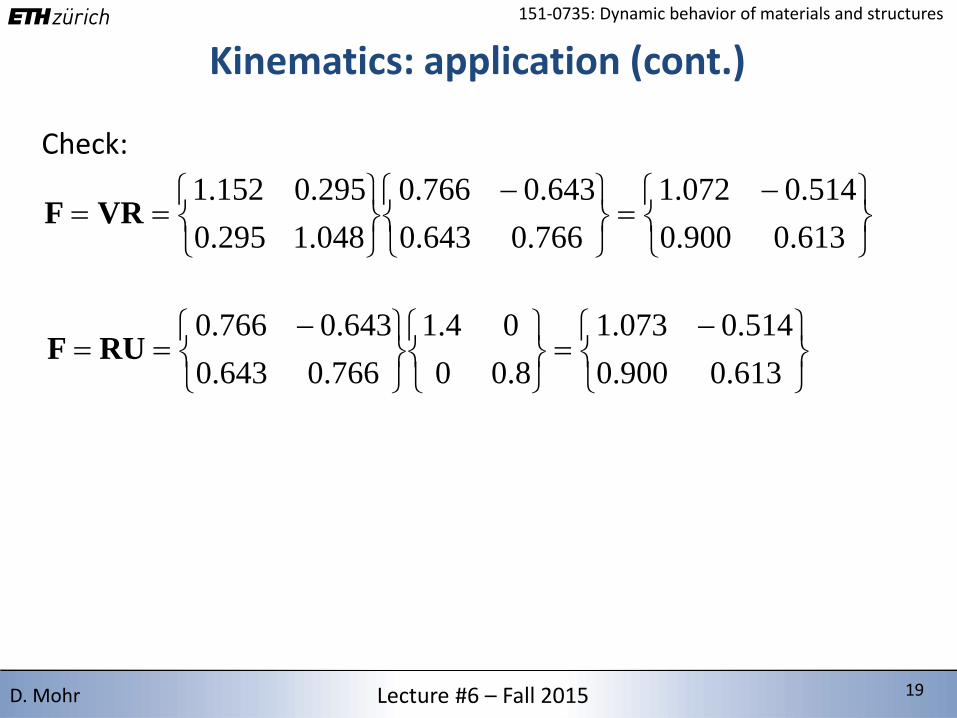
Kinematics: application (cont.)
VRRUF TRURRURV 1
766.0643.0
643.0766.0
8.00
04.1
766.0643.0
643.0766.0V
048.1295.0
295.015.1
766.0643.0
643.0766.0
613.0900.0
512.0073.1
2211
2211
1
8.04.1
8.04.1
ReReReRe
ReeeeRRURRURV
TT
Spectral decomposition:
413.0492.0
492.0587.011 ReRe
587.0492.0
492.0412.022 ReRe

2/15/2016 18 18Lecture #6 – Fall 2015 18D. Mohr
151-0735: Dynamic behavior of materials and structures
Kinematics: application (cont.)
048.1295.0
295.0152.1
587.0492.0
492.0412.08.0
413.0492.0
492.0587.04.1
8.04.1 2211 ReReReReV
Spectral decomposition (cont.):
413.0492.0
492.0587.011 ReRe
587.0492.0
492.0412.022 ReRe
008.0276.0
276.0105.0
587.0492.0
492.0412.0]8.0ln[
413.0492.0
492.0587.0]4.1ln[
8.04.1ln 2211 ReReReReV
2/15/2016 19 19Lecture #6 – Fall 2015 19D. Mohr
151-0735: Dynamic behavior of materials and structures
Kinematics: application (cont.)
613.0900.0
514.0072.1
766.0643.0
643.0766.0
048.1295.0
295.0152.1VRF
Check:
613.0900.0
514.0073.1
8.00
04.1
766.0643.0
643.0766.0RUF

2/15/2016 20 20Lecture #6 – Fall 2015 20D. Mohr
151-0735: Dynamic behavior of materials and structures
][cos][sin
][sin][cos][
tt
ttt
R
Rotation
][5.010
0][1][
tu
tutU
RUF
Stretching
1
1
1.2
0.9
1.4
0.8
1
1
20⁰ 40⁰
u[t] increases linearly from 0 to 0.4 [t] increases linearly from 0 to 40°
Kinematics in Abaqus/explicit
2/15/2016 21 21Lecture #6 – Fall 2015 21D. Mohr
151-0735: Dynamic behavior of materials and structures
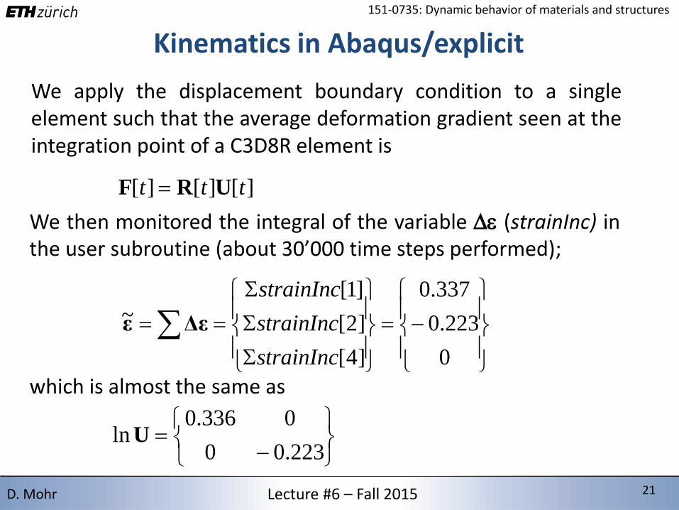
Kinematics in Abaqus/explicit
We apply the displacement boundary condition to a singleelement such that the average deformation gradient seen at theintegration point of a C3D8R element is
][][][ ttt URF
We then monitored the integral of the variable D (strainInc) inthe user subroutine (about 30’000 time steps performed);
0
223.0
337.0
]4[
]2[
]1[~
strainInc
strainInc
strainInc
Δεε
223.00
0336.0ln U
which is almost the same as

2/15/2016 22 22Lecture #6 – Fall 2015 22D. Mohr
151-0735: Dynamic behavior of materials and structures
Abaqus/explicit user material (VUMAT) interface
However, the Abaqus CAE output variable LE is different. For thesame simulation, we find
551.0
008.0
105.0
12
22
11
LE
LE
LE
which is almost the same as
008.0276.0
276.0105.0ln V
Note that the shear component of LE is twice that of lnV whichis due to the difference between the mathematical andengineering definition of shear strains.

2/15/2016 23 23Lecture #6 – Fall 2015 23D. Mohr
151-0735: Dynamic behavior of materials and structures
Abaqus/explicit user material (VUMAT) interface
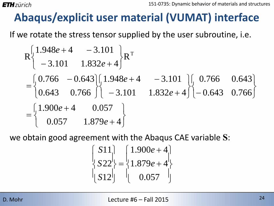
For the same simulation, the Abaqus CAE output variable Sreads
2684.5
4879.1
4900.1
12
22
11
e
e
e
S
S
S
While the stress variable supplied by the subroutine is
101.3
4832.1
4948.1
]4[
]2[
]1[
e
e
stressNew
stressNew
stressNew
2/15/2016 24 24Lecture #6 – Fall 2015 24D. Mohr
151-0735: Dynamic behavior of materials and structures
Abaqus/explicit user material (VUMAT) interface
If we rotate the stress tensor supplied by the user subroutine, i.e.
4879.1057.0
057.04900.1
766.0643.0
643.0766.0
4832.1101.3
101.34948.1
766.0643.0
643.0766.0
R4832.1101.3
101.34948.1R T
e
e
e
e
e
e
057.0
4879.1
4900.1
12
22
11
e
e
S
S
S
we obtain good agreement with the Abaqus CAE variable S:

2/15/2016 25 25Lecture #6 – Fall 2015 25D. Mohr
151-0735: Dynamic behavior of materials and structures
Abaqus/explicit user material (VUMAT) interface
1nF
1nU
1nR
INITIAL
DEFORMED @ tn+1
STRETCHED @ tn+1
(stretched & rotated)
Stress tensor to be provided by VUMAT subroutine
1~
nσ
n~
nσt ~~~1 n
nRn ~1 n
nσt 1 n
Cauchy stress tensor (variable S in CAE)
t
nnnn 1111~
RσRσ
Strain tensor in user subroutine
D1
1
1 ]ln[~n
i
in Uε
Strain tensor (Variable LE in CAE)T
nnnn 1111~
RεRε
*The above relationships are still schematic approximations of the “real” kinematics computations performed by Abaqus/explicit

2/15/2016 26 26Lecture #6 – Fall 2015 26D. Mohr
151-0735: Dynamic behavior of materials and structures
Exercise: total strain integration
The total strain obtained after summing the strain increments,
D1
1
1 ]ln[~n
i
in Uε
may be different from that obtained from the total strain definition
]ln[~11 in Uε
If the principal axes of the stretch tensor remain unchanged duringthe entire loading path, both definitions are identical, i.e.
]ln[]ln[ 1
1
1
D i
n
i
i UU

2/15/2016 27 27Lecture #6 – Fall 2015 27D. Mohr
151-0735: Dynamic behavior of materials and structures
Now, consider for example a rotation-free two-step loadingcomprised of
D8.00
011U
D12.0
2.012Ufollowed by
The total stretch applied is
DD8.02.0
16.0112 UUUtot
1
1
1
0.8
1UD 2UD
Exercise: total strain integration

2/15/2016 28 28Lecture #6 – Fall 2015 28D. Mohr
151-0735: Dynamic behavior of materials and structures
The spectral decompositions of the stretch tensors are
D1
0
1
08.0
0
1
0
10.1
8.00
011U
D707.0
707.0
707.0
707.08.0
707.0
707.0
707.0
707.02.1
12.0
2.012U
886.0
465.0
886.0
465.0695.0
548.0
836.0
548.0
836.0105.1
8.02.0
16.01totU
Exercise: total strain integration

2/15/2016 29 29Lecture #6 – Fall 2015 29D. Mohr
151-0735: Dynamic behavior of materials and structures
and the corresponding logarithmic strain tensors are
D
223.00
00]ln[ 1U
D
020.0203.0
203.0020.0]ln[ 2U
]ln[]ln[255.0195.0
195.0009.0]ln[ 21 UUU DD
tot
DD
243.0203.0
203.0020.0]ln[]ln[ 21 UU
which provides an illustration of the small error associated with theincremental strain definition .
Exercise: total strain integration
2/15/2016 30 30Lecture #6 – Fall 2015 30D. Mohr
151-0735: Dynamic behavior of materials and structures
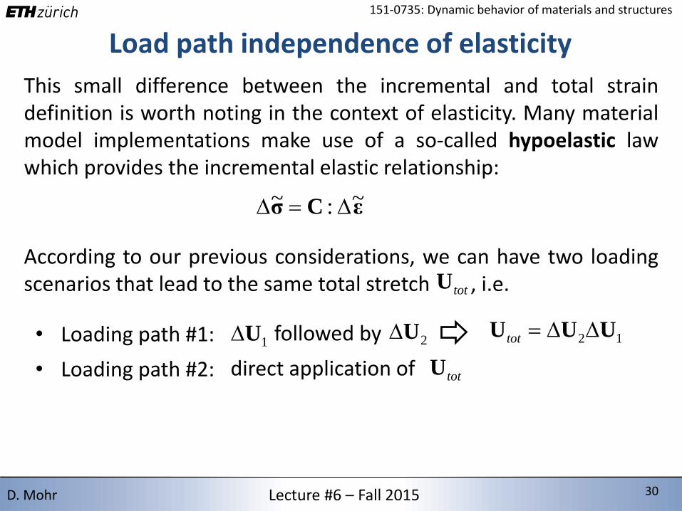
This small difference between the incremental and total straindefinition is worth noting in the context of elasticity. Many materialmodel implementations make use of a so-called hypoelastic lawwhich provides the incremental elastic relationship:
εCσ ~:~ DD
According to our previous considerations, we can have two loadingscenarios that lead to the same total stretch , i.e.
• Loading path #1: 12 UUU DDtot1UD
totU
followed by 2UD
• Loading path #2: direct application of totU
Load path independence of elasticity

2/15/2016 31 31Lecture #6 – Fall 2015 31D. Mohr
151-0735: Dynamic behavior of materials and structures
Even though both loading scenarios lead to the same stretch, theapplication of the incremental hypoelastic law would result indifferent stresses:
]ln[]ln[:]ln[:]ln[:~21211 UUCUCUCσ DDDD
This inequality violates the basic principle of loading pathindependence of elasticity. Note that this error is associated withthe integration of the total strain. However, for the sake ofcomputational efficiency, this small error is widely accepted inindustrial practice (and even in academia).
• Loading path #1:
• Loading path #2:
12~]ln[:~ σUCσ tot
Load path independence of elasticity

2/15/2016 32 32Lecture #6 – Fall 2015 32D. Mohr
151-0735: Dynamic behavior of materials and structures
To avoid any artificial path dependency of the elastic response in FEcomputations, it is recommended to compute the total stretchtensor through polar decomposition of the current deformationgradient.
RUF
And then compute the associated stress tensor
Load path independence of elasticity
3
1
22 )()(i
iii
TuuUFF
3
1
)](ln[ln~
i
iii uuUε
)~~(:~2 pεεCσ
Note that the plastic strain is just included for completeness in the above elasticconstitutive equations. It has been zero in the examples considered above.

2/15/2016 33 33Lecture #6 – Fall 2015 33D. Mohr
151-0735: Dynamic behavior of materials and structures
Pressure-dependent plasticity

2/15/2016 34 34Lecture #6 – Fall 2015 34D. Mohr
151-0735: Dynamic behavior of materials and structures
In solid mechanics, the pressure is defined as
)(3
1
33
][ 1IIIIII
Itrp
σ
Stress tensor decomposition
It characterizes the hydrostaticpart of the Cauchy stress tensor:
= +
HYDROSTATIC PART(average stress)
DEVIATORIC PART(differences among stresses)
𝛔𝐈
𝛔𝐈𝐈
𝛔𝐈𝐈𝐈
−𝒑
(𝛔𝐈𝐈𝐈+𝒑)
(𝛔𝐈 + 𝐩)
(𝛔𝐈𝐈+𝒑)
−𝒑
−𝒑
1Sσ p

2/15/2016 35 35Lecture #6 – Fall 2015 35D. Mohr
151-0735: Dynamic behavior of materials and structures
Isotropic yield functions can be conveniently expressed in terms ofthe pressure (or first invariant of the stress tensor) and theinvariants J2 and J3. of the deviatoric stress tensor:
Von Mises yield function
],,[ 321 JJIff
Due to the proportionality of p and I1, the pressure dependence of ayield function is characterized through its dependence on the firstinvariant I1. The von Mises function is a typical example of apressure-independent yield function.
22 3][ JJff vMvM

2/15/2016 36 36Lecture #6 – Fall 2015 36D. Mohr
151-0735: Dynamic behavior of materials and structures
The Drucker-Prager yield function is a first extension of the vonMises yield function assuming a linear pressure dependence:
Drucker-Prager yield function
It is applicable to mildly porous metals (cast iron), concrete or steelat very high pressures.
1221 3],[ aIJJIff DPDP

2/15/2016 37 37Lecture #6 – Fall 2015 37D. Mohr
151-0735: Dynamic behavior of materials and structures
Illustration
Initial
ep
Hydrostatic pressure Hydrostatic pressure plus axial loading
ep
ep
ep
• Compression experiments under hydrostatic pressure

2/15/2016 38 38Lecture #6 – Fall 2015 38D. Mohr
151-0735: Dynamic behavior of materials and structures
Effect of hydrostatic pressure on the stress-strain response of 4330steel:
Illustration: Results from Richmond and Spitzig (1980)

2/15/2016 39 39Lecture #6 – Fall 2015 39D. Mohr
151-0735: Dynamic behavior of materials and structures
• Effect of hydrostatic pressure on the stress-strain response of4330 steel:
Illustration: Results from Richmond and Spitzig (1980)
kaIJJIfDP 1221 3],[
)( 1 MPaI
)(
2M
Pa
J

2/15/2016 40 40Lecture #6 – Fall 2015 40D. Mohr
151-0735: Dynamic behavior of materials and structures
Reading Materials for Lecture #6
• M.E. Gurtin, E. Fried, L. Anand, “The Mechanics and Thermodynamics of Continua”, Cambridge University Press, 2010.
• Abaqus Theory Manual abaqus.ethz.ch:2080/v6.11/pdf_books/THEORY.pdf
• O. Richmond and W.A. Spitzig,,“Pressure dependence and dilatancy of plastic flow”, IUTAM Conference, ASME, 1980, p. 377


![C5.2 Elasticity and Plasticity [1cm] Lecture 5 Plane strain](https://img.dokumen.tips/doc/110x75/625d199f7a3aa731631d9e64/c52-elasticity-and-plasticity-1cm-lecture-5-plane-strain.jpg)


![C5.2 Elasticity and Plasticity [1cm] Lecture 2 Equations](https://img.dokumen.tips/doc/110x75/622f8f3994946046a5727b7b/c52-elasticity-and-plasticity-1cm-lecture-2-equations-.jpg)


