97

Lecture 5: Random numbers and Monte Carlo

(Numerical Recipes, Chapter 7)

• Motivations for generating random numbers– To sample a function in a statistically

controlled manner (i.e. for Monte Carlo integration)

– The simulate truly random processes (noise, radioactive decay …)

98

Random number generators

• Obvious problem: computers are deterministic.– Computer generated random numbers aren’t

truly random: given a known starting point, any sequence can be predicted

– Best we can achieve is pseudo-randomsequences with certain statistical properties

99

Hardware devices can produce truly random numbers

Rely on thermal noise to produce several x 105 random numbers / second – cryptographic applications

100

Random number generators• Typical generator: creates a sequence of

numbers, rk, distributed uniformly over the interval [0,1]– Start with a seed value: each seed creates a different

sequence of integers, Ik, over the interval [0,M]– These integers are used to create floating-point

numbers, rk = float (Ik)/float(M) over the interval [0,1]– Typical generator is portable: yields same result on

any machine (important for error-checking)– The sequence will inevitably repeat with a period

P ≤ M

101

Random number generators

• We want to minimize correlation functions:

Define AL = < (rk – 0.5) (rk+L – 0.5) >where < > denotes an average over all k

Truly random numbers would have AL = 0 for all L

Clearly, real random number generators have AL > 0 whenever L is a multiple of P

… and many have some correlations even when L < P

102

Random number generators• Linear congruential generators:

Ij+1 = (a Ij + c) mod M with M, a and c (carefully chosen) fixed integers(“Minimal Standard” routine: M = 231 – 1, a = 75, c = 0)

Problems:Clearly, the period P is at best M (and – for poorly chosen a and c –

can be much less than M)Correlations for small l:

e.g. in above example, rk < 10–6 always followed by rk +1 < 0.0168

von Neumann: “Anyone who uses arithmetic methods to produce random numbers is in a state of sin."

103

Random number generators

• Problems fixed by the use of a “shuffle box”

From Numerical Recipes

104

Non-uniform probability distributions

• So far, we have consider the generation of random numbers with a “top-hat” probability distribution

p(x) = 1 (0 < x < 1)p(x) = 0 (otherwise)

x

p(x)

1

1

0

105

Non-uniform probability distributions

• Suppose we want a different distribution function, q(y)– solution: generate x as before and take y = f(x)

• What function f is required?We want the probability that y lies between y and y+dyto equal q(y) dy

This is the probability that x lies between f –1 (y) and f –1 (y+dy), which is simply | f –1(y+dy) – f –1(y) | = | df –1(y) /dy | dy

Hence the required function has inverse f –1 = ∫ -∞y

q(z) dz

106

Non-uniform probability distributions

• Example: suppose we want an exponentially distributed sequence of random numbers (to simulate the lifetimes of radioactive nuclei)

q(y) = (1/τ) e–y/τ (for τ ≥ 0, and = 0 otherwise)

f –1(y) = ∫0y

(1/τ) e–z/τ dz = (1 – e–y/τ )

for which the inverse is y = f(x) = – τ ln (1 – x)

107

The rejection method

• Another way of producing a desired distribution of random variables, q(y), is to choose 2 uniformly distributed random #s, a1 and a2, in the interval [0,1]

• Take y = ymin + a1 (ymax – ymin)z = a2 qmax

If z < q(y), keep yIf z > q(y), discard yThe remaining set of y-value has the desired probability

distribution

108

The rejection method• Picture:

q(y)

yymin ymax

keep

reject

109

Numerical root finding(Numerical Recipes, Chapter 7)

• A basic problem in mathematics: solve an equation g(x) = y

• Convenient convention: rewrite this is f(x) = 0• The solutions are called the roots of f

f(x)

x

110

Numerical root finding

• We can also have a multidimensional problem in which coupled sets of equations must be solvedf1(x1, x2, …) = 0

f2(x1, x2, …) = 0 f(x) = 0……

(Just spent two lectures doing this for the linear case A x – b = 0. MUCH harder for the general multi-D non-linear case; will discuss this more later, but first let’s look at the 1-D non-linear case, f(x) = 0)

111

Bracketing

• How do you know if a root exists?If there a no singularities, then if you can find an interval [a,b] such that f(a) and f(b) have opposite signs, there must be at least one root between a and b

Establishing such an interval is called “bracketing”Root finding without a bracket is tricky

112

Bracketing

• If there are no singularities, there must be a root between a and b

f(x)

x

f(a) < 0

f(b) > 0

113

Root finding algorithms

• All root finding algorithms are iterative need a good guess (or small bracket) as a

starting point

Like numerical integration, we need to know something about our problem to create an optimal solution: making a graph never hurts

114

Root finding algorithms

• In the 1-D case, there is a tradeoff between speed and robustness

• Slower methods maintain a bracket at all times (bisection, “false position”) – successive iterations simply contract the bracket

• Faster methods do not maintain a bracket and can shoot unstably away from the root (Newton-Raphson, “secant”)

• Hybrid methods seek to get the best of both worlds (Brent, Ridder, “safe Newton-Raphson”)

115

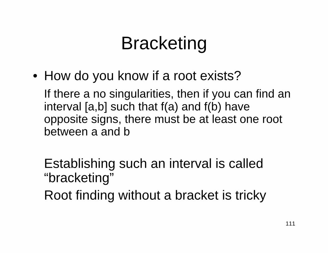
Bracketing

• A bracket is usually sufficient, although a singularity is still possible: e.g. f(x) = (x – c)–1

f(x)

xcf(a) < 0

f(b) > 0

Fortunately, no danger ofmistaking this for a root!

116

Bracketing

• The absence of a bracket can imply any number of roots

f(x)

x

f(a) > 0 f(b) > 0

117

Finding an initial bracket

• Recipes describes and provides two bracket-finding routines:

• ZBRAC: expands a seed interval looking for a bracket

• ZBRAK: subdivides a seed interval looking for brackets (good for multiple roots)

118

Pathologies• Some functions have roots, but it is impossible to find

bracketse.g. Recipes equation (3.0.1)

0 = f(x) ≡ 3x2 + (1/π4) ln [(x – π)2] + 1

Has a weak singularity at x = π, two roots very near x = π, but is negative only in the interval x = π ± 10–667

You will probably never find a bracket even in quad precision

119

Pathologies• Some functions have infinitely many roots over a finite

range, e.g. f(x) = sin(1/x)

• MORAL: understand your function before jumping into a numerical solution

From Recipes, Fig 9.1.1

120

Root finding algorithms: bisection

• Once you have found a bracket, it can always be narrowed using the bisection method:– Divide [a,b] into [a , ½(a+b)] and [½(a+b), b]– Keep the valid bracket and repeat until the

interval reaches a preset size – Totally foolproof – will also find singularities if

they exist

121

Performance of bisection

• In bisection, the size of the bracket after n iterations is εn = ½ εn–1

• This is called linear convergence, because εn ∝ (εn–1)m with m = 1

• Faster methods have m > 1 and have “supralinear” convergence

122

Performance of bisection

• Note that linear convergence isn’t at all bad: we still have εn = 2–n ε0

• Number of interations needed to achieve precision ε is log2 (ε0/ε)

• Need to quit anyway when ε approaches machine accuracy (for which n might typically be ~ 40 in double precision)

123

Secant and false position methods

• Bisection only makes use of information about the sign of the function. We can do better if we consider also the magnitude

• The secant and false position methods both use linear interpolation to decide how to narrow the bracket– False position always maintains a valid bracket– Secant doesn’t necessarily, and is therefore less

robust (but faster)

124

Geometric representation• Secant method:

picture from Recipes, showing how an initial interval [1,2] is narrowed to [1,3] and then to [4,3]

• Convergence is supralinear, with m = 1.618

Extrapolate or interpolate from two mostrecently evaluated points

125

Geometric representation• False position method:

picture from Recipes, showing how an initial bracket [1,2] is narrowed to [1,3] and then to [1,4] as necessary to maintain a valid bracket

• Convergence is somewhat supralinear, with 1< m < 1.618 depending upon the exact function

Interpolate between the two mostrecently evaluated points that bracket the root

126

Pathologies • Neither secant nor false

position works very well in all circumstances: example using false position from Recipes Fig 9.2.3[1,2] [3,2] [4,2] …..

• In this case, bisection would be much better

127

Brent’s method(Van Wijngaarden-Dekker-Brent method developed in 1960s)

• Hybrid method which is generally the method of choice for 1-D functions*

• Improvements over false secant method– Using quadratic interpolation using three

previously calculated points– Switches to bisection when that proves faster

• Faster convergence for well-behaved functions

• Always does at least as well as bisection*unless the derivative is known: see Newton-Raphson