Lecture 5: Guiding mechanisms - RWTH Aachen … machine tool ... Quasi-static study of a ... optimisation of the guide systems with regard to the stiffness, the static and dynamic

Lecture 5:

Guiding mechanisms

Person-in-charge: Dipl.-Ing. Florian Lindner

Steinbachstraße 54 A

Room 304

Tel.: 0241 / 80 - 26287

E-mail: [email protected]

Virtual machine tool – Modelling and Simulation Lecture: Guiding mechanisms V5-1

AACHEN

© WZL

F. P

aepe

nmül

ler

D

atei

: Virt

uelle

WZ

M F

olie

n en

gl 1

-5.d

sf

Bild

num

mer

: V6-

1eFunctions of Guideways and Bearings

functions

- connecting parts moving relatively to each other- exact, linear motion along one axis- carry mass forces- carry process forces

requirements

- low wear- low friction- high working precision- high stiffness- high damping- low costs

element with6 degrees of freedom

translational: x, y, zrotational: αx, αy, αz

milling machine slide lathe spindle

5 blocked degrees of freedomremaining: y

5 blocked degrees of freedomremaining: αx


Functions of guides and bearings

The guiding mechanisms of machine axes, workbenches and handling facilities as well as bearings of the main spindles are part of the most important components in the power flow of a machine tool. Thereby, bearings and guides have the task of reducing the degree of freedom of a technical system in motion. Basically, all movements in the space can be created through translation and rotation, i.e. the current six degrees of freedom are reduced on a displacement along an axis or on a rotation at an axis respectively. Thus, e.g. a straight slide has only one translatory degree of freedom, while the mandrel contains only one rotary degree of freedom, as shown in illustration 1.

For the following models, it is defined that the coupling positions of components that permit a rotation, are called ‘bearings’. Translatory relative motions are guaranteed by ‘guides’.

Essentially, guides must guarantee a high working precision at low production and operating costs. To fulfil these demands, guiding mechanisms and bearings have the following properties:

- low wear to guarantee the precision

- low friction and stick-slip freedom as prerequisite for exact positioning at low advance forces

- high stiffness and clearance to keep the position changes under load low

- good damping in carrying and motion direction to avoid overshooting of feed drives and chattering of the machine

Moreover, these components are in the direct flow of power of the machine tools and therefore must absorb any weight, acceleration and machining forces. Thus, e.g. machining powers initiated through

the tool are transferred to the coupling positions on the various structure components.


AACHEN

© WZL

F. P

aepe

nmül

ler

D

atei

: Virt

uelle

WZ

M F

olie

n 1-

5.ds

f

B

ildnu

mm

er: V

6-2

Use of Guideway Systems in Machine Tools

guideway X-axistool changer

guidewayY-axis

guideway X-axis

guidewayW-axis

guideway Z-axis

guideway Z-axistool changer

guidewayspindle changer


Use of guide systems in machine tools

Guides and guide systems are used in all areas of the machine tool construction and handling. Illustration 2 shows the areas of use for guide systems with the example of a portal machine for machining large parts.

The machine table guided in x-direction is frequently provided with sliding guides in a machine of this size, which is arranged below the guideway cover. Sliding guides and rolling guides are used for the w, y and z-axes. Guiding mechanisms are used for the actual guide of the machine tool axes, which satisfy the highest requirements with regard to stiffness and precision.

For accessory parts, such as the spindle control and the tool changer, the requirements with regard to the stiffness and precision are less important. In view of short tool changing times, high possible path feed rates and accurate positioning are at the foreground here.

Numerous variants of guide systems have come into the market due to the various requirements, which are tuned to the guiding task (precision, speed, stiffness, etc.).


AACHEN

© WZL

F. P

aepe

nmül

ler

D

atei

: Virt

uelle

WZ

M F

olie

n 1-

5.ds

f

B

ildnu

mm

er: V

6-33

Simulation and Dimensioning of Guideway Systems

calculation goal

- life span (in hours oder km)- load bearing capacity

- stiffness of the guideway system - stiffness of the machine

- damping and dynamic / vibration behaviour

effects

- component failure

- machine accuracy- imperfect shape of the workpiece

- machine accuracy - chatter marks on the work piece

restricted :

chatter marks on acrankshaft

carriage destroyed by dirt and overload

model of a statically deformed machine tool


Simulation and calculation of guideway systems

The calculation and simulation of machine tools and their components primarily have the task of determining the static and dynamic operating performance already in the design phase.

In view of accurate and reliable machines, the components must be dimensioned in such a way that the accepted properties in view of life and efficiency (e.g. carrying capacity of the guide system) are achieved. Under-dimensioning can cause early component malfunctions, which in case of guide systems also always leads to machine breakdown. The calculation facilitates information on the life of guide systems in path feed lengths (km) or operating hours in dependence of a specific load collective, which corresponds to the later machine load. In addition, extended calculation models acquire various lubrication states. It is not possible to consider the effects of dust (chips, wood dust, cooling lubricant, etc.).

In order to minimise faults in later operation during the machining of parts, one must strive for a rigid machine design. The selection and design of guide systems can have a larger influence on the static machine behaviour. The dimensioning of the guide systems, the selection of the guiding principle and the arrangement of guides on the machine are the main simulation tasks.

In addition to the static machine properties that evoke shape faults on the workpiece, even dynamic machine instabilities can cause workpiece faults (clattering) or even damages to the machine. In order to identify and minimise the instabilities already in the design process, dynamic simulations and calculations are used, e.g. the Multi-Body Simulation (MKS) or the determination of the natural oscillation shapes with dynamic Finite Element analysis. The mechanical vibration behaviour can be influenced positively by damping elements in the machine design. Damping can be realised

especially in the coupling positions (threaded joints and guide systems) by converting vibration and friction energy. By selecting the guide principle, principle-related damping properties can be used. The precise vibration ratios could not be satisfactorily simulated until now due to the complex boundary conditions (lubrication, damping constants of the coupling positions), so that here an adjustment with measurements on the real machine must be carried out.


yx

z

K1

K2

K3K4

K5

K6K7

K9K8

E5

E1

E2

E4

E6

E7

E8

AACHEN

© WZL

F. P

aepe

nmül

ler

D

atei

: Virt

uelle

WZ

M F

olie

n en

gl 1

-5.d

sf

Bild

num

mer

: V6-

3eQuasistatic Test of a Machining Center (z-Direction)

elementscouplingpoints

overallcomplianceratio (%)

bed

x guideway

y guideway

z guideway

compound slide

column

spindle box

spindle

E1

E3

E4

E6

E2

E5

E7

E8

100%=0,026 µm/N

K1, K2

K3, K4

K4, K5

K6, K7

K2, K3

K5, K6

K7, K8

K8, K9

0

0

54

15

11

0

17

6E3


Quasi-static study of a machining center (z-direction)

Illustration 3 shows the displacements of a machining center, which were determined with a quasi-static study through measurements. The quasi-static study helps to determine the ratio of components on the static total deformation. To do that, the machine with stochastic power signals is stimulated on the tool and the dislocations of the machine components are recorded. As long as the displacements are carried out in balance with the power initiation (phase angle ϕ=0°), one implies quasi-static behaviour.

The measurement clearly shows that the coupling positions of the guides cause the largest portion with distance on the total displacement. The y-axis guide has the largest portion with 54%. The low support length of the y-guide system and the big power initiation lever arm required by the position of the spindle box causes this result. Other clear portions on the displacement have the guides of the x and z axes. The frame components, except the spindle box are designed very rigid, so that no proportionate displacements occur at these positions. The coupling positions in the milling spindle (spindle bearing) have only one comparatively lesser portion on the total displacement.

The flexible design of the y-guide together with the large mass of the machine column can mean that the machine at this position can show dynamic instabilities already at low frequencies. In finished machines, improvements of properties cannot be converted or only limitedly and always involve high costs and much work.

During the design process, the weak points can be identified early. With an altered arrangement of the y-support length and an optimisation of the guide systems with regard to the stiffness, the static and dynamic properties of the complete machine and subsequently their precision behaviour can be improved.


AACHEN

© WZL

F. P

aepe

nmül

ler

D

atei

: Virt

uelle

WZ

M F

olie

n en

gl 1

-5.d

sf

Bild

num

mer

: V6-

4ePhysical Principles of the Guiding and Bearing Systems

oil storage tank

slide

hydrodynamicslideway and plain bearing

aerostaticslideway

and plain bearing

air pressuresystem

hydraulicsystem

hydrostaticslideway

and plain bearing linear ballguidance system

and ball bearing

electromagneticbearing

rotor with plates

iron ring

coil

position sensor


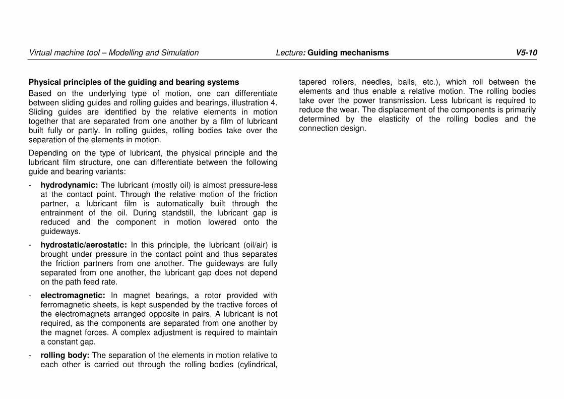
Physical principles of the guiding and bearing systems

Based on the underlying type of motion, one can differentiate between sliding guides and rolling guides and bearings, illustration 4. Sliding guides are identified by the relative elements in motion together that are separated from one another by a film of lubricant built fully or partly. In rolling guides, rolling bodies take over the separation of the elements in motion.

Depending on the type of lubricant, the physical principle and the lubricant film structure, one can differentiate between the following guide and bearing variants:

- hydrodynamic: The lubricant (mostly oil) is almost pressure-less at the contact point. Through the relative motion of the friction partner, a lubricant film is automatically built through the entrainment of the oil. During standstill, the lubricant gap is reduced and the component in motion lowered onto the guideways.

- hydrostatic/aerostatic: In this principle, the lubricant (oil/air) is brought under pressure in the contact point and thus separates the friction partners from one another. The guideways are fully separated from one another, the lubricant gap does not depend on the path feed rate.

- electromagnetic: In magnet bearings, a rotor provided with ferromagnetic sheets, is kept suspended by the tractive forces of the electromagnets arranged opposite in pairs. A lubricant is not required, as the components are separated from one another by the magnet forces. A complex adjustment is required to maintain a constant gap.

- rolling body: The separation of the elements in motion relative to each other is carried out through the rolling bodies (cylindrical,

tapered rollers, needles, balls, etc.), which roll between the elements and thus enable a relative motion. The rolling bodies take over the power transmission. Less lubricant is required to reduce the wear. The displacement of the components is primarily determined by the elasticity of the rolling bodies and the connection design.


AACHEN

© WZL

F. P

aepe

nmül

ler

D

atei

: Virt

uelle

WZ

M F

olie

n en

gl 6

-10.

dsf

Bild

num

mer

: V6-

6eApplication Examples - Hydrostatic Guides

hydrostatic slideway of agear shaping machine

hydrostatically supported machine slide

clamping bar

low-profileguideway

guide rail

wrap-around

raceway

seal

capillary

upper ram

guideway

lower ram guidewayram guideway for the

tilting movement


Application examples – Hydrostatic guides

The illustration shows the cross-section through a hydrostatic machine slide on bearings. To calculate the displacement, one uses suitable digital computing programs. By considering all the recesses, the equilibrium conditions are placed, which produce the local displacements and the inclination of the slide. Often, the elastic behaviour of the frame components and the modified parts must be taken into consideration in the calculation, as the effective gaps are acquired only in this manner and the total displacements can be determined exactly.

Another application example, the hydrostatic guide of the ram and the ram head of a gear-shaping machine for producing gears is illustrated. To prevent the static and motional friction from changing during the ram movement, the hydrostatic is especially advantageous here. The upper guide serves as longitudinal guide of the ram for the up and down movement. This guide also transfers the rotation initiated through helix and worm wheel. The lower guide comprises of a single circular guide of the ram and a single flat guide of the ram head. The flat guide is required for the tilting lifting motion of the tool during return stroke.


AACHEN

© WZL

F. P

aepe

nmül

ler

D

atei

: V

irtue

lle W

ZM

Fol

ien

engl

6-1

0.ds

f B

ildnu

mm

er V

6-7e

Application Examples - Roller Guides

source: WZL, Schneeberger

fitting strip

V-ledge linear roller bearing

columnguide rail

machine bed

ball bearingspindle

machinebed

linear ball guidance system with profiled rails

measuringsystem


Application examples – Roller guides

Illustration 7 shows two typical applications for rolling guide systems. A typical machine column guide is built from roller recirculation bushes, which run on hardened guide rails. In order to absorb traction and pressure forces, the roller recirculation bushes are arranged opposite in pairs (so-called system with wrap-around). The required clearance and initial stress is set through ground fitting strips. The lateral guide is likewise realised with roller recirculation bushes that are arranged on both sides of the guide rail. By twisting the adjusting screw on the V-ledge, two wedge surfaces are shifted against each other and the required initial stress is defined.

The illustration on the right shows the typical arrangement of linear guiding systems for the linear axes of a machine tool. The columns and slides move on a guiding system comprising of rails and guide carriages. The carriages are fixed with revolving ball and rolling elements. The advantage of this system is that the components can be referred as standardised catalogue-ware, are pre-stressed and ready for use and are lubricated. If damaged, they are easy to replace.


AACHEN

© WZL

F. P

aepe

nmül

ler

D

atei

: Virt

uelle

WZ

M F

olie

n en

gl 6

-10.

dsf

Bild

num

mer

: V6-

8eComponents of a Ball Monorail Guidance System

source: Bosch Rexroth AG

8

1 - screwing plate2 - sealing3 - cover4 - ball reversing unit5 - lubrication unit6 - ball chain (4-row)7 - carriage8 - rail


Components of a ball monorail guidance system

Circulating guides with ground rail profile are used very often in machine tool construction. With the example of a four-row system in illustration 8, the structure of a ball rail guide is explained.

A profile rail guidance system essentially comprises of the guide rail (8) and the carrier or guide carriages (7), in which the rolling bodies (6) are integrated. In illustration 8, the balls are embedded in a chain made of flexible plastic, which holds the balls at defined distance and comes with lubricating recesses. However, even systems without additional rolling body retainers are used. The balls enter the loading zone on one side between rails and carriages, run through them and are thereafter turned around in the carriage by means of a deflecting piece (4) and redirected to the loading zone. The deflecting pieces are held by the cover (3) and the joint sheet (1) on the carrier. To protect the system from chips and cooling lubricant, a plastic seal is provided in the cover that prevents dust particles from penetrating. Through a connection on the front side, the rolling bodies are equipped with lubricant (oil or grease). To increase the lubricating interval, some manufacturers provide the systems with lubricant tanks (5) that are supposed to deliver the lubricant slowly to the rolling body.

Dimensions and capacity calculations for profile rail rolling guides are standardized (DIN 636 and DIN 645). The guiding systems are delivered ready for installation. The machine manufacturer can generally choose from various precision classes (height, width tolerance), pre-stress classes (play encumbered, no-play, medium and high pre-stress), lubricant supply (grease, oil-impulse, oil-air lubrication), as well as sealing and stripping systems. From the single components, one can assemble such a system that is matched optimum to the load and ambient conditions.


AACHEN

© WZL

F. P

aepe

nmül

ler

D

atei

: Virt

uelle

WZ

M F

olie

n en

gl 6

-10.

dsf

Bild

num

mer

: V6-

9eKinematics of Rolling Guides

guid

eway

s

ball

roller / needle (l>>d)

point contact

line contact

two-point contact

four-point contact

l

d

flat surface

bearing surface with raceway

curvature

compound roller arrangement

row arrangement


Kinematics of rolling guides

Rolling guide systems are identified by the fact that the rolling bodies ensure the relative motion of the components moved together. Balls, rollers and pins are always used as rolling body geometries.

On the contact of a ball with a plane bearing surface, the contact forces are transmitted on a very small surface (point contact). The contact surfaces can be increased (bevelling) through the concave formation of the bearing surface and subsequently the local pressing.

Multi-row ball wraparound guides are designed with a 2 point contact. Like in deep groove ball bearings, the tracks show a narrow bevelling, which ensure the highest possible carrying capacity and stiffness per row of balls. Forces can only be transmitted in a limited pressure angle range. By using multiple rows of balls with various pressure angles, the guides can be matched with the application areas.

Ball wraparound guides with a 4 point contact have tracks with Gothic arcs. The bevelling is bigger than in 2 point contact. In compact size, high loads can be transmitted through a large pressure angle range.

Rollers and pins transmit the forces through line contact. Based on the larger bearing surface and the pressing reduced with that, the carrying capacity of these systems is clearly over those of balls. Pins are identified by the fact that the pin length is essentially bigger that the pin diameter (l/d>>2). To avoid tipping (crowning) of the pins on the bearing surface, the pins are normally directed to an additional cage. Cylindrical roller bodies can either be arranged in one level (row arrangement) or in two inclined levels to absorb forces from various directions (cross-roller arrangement or V-arrangement).

In addition, modifications of this basic rolling body shapes are also used, e.g. crowned rollers or barrels.


AACHEN

© WZL

Inner Force Ratios at Different Rolling Body Arrangement

C

symmetric asymmetric

offset

tension compression

C

C

C tension compressionCcompressionC C tension offsetCoffsetC

C tension compressionC

FV

FV FV FVα N WK

=

plane of symmetryin between theroller bodies

offsetC

2

1

FVN1

= = > >

FVN1

d

d+∆d

d

d+∆d

principle of preloading

F. P

aepe

nmül

ler

D

atei

: Virt

uelle

WZ

M F

olie

n en

gl 6

-10.

dsf

Bild

num

mer

: V6-

10e


Inner force ratios at different rolling body arrangement

Characteristic ranges for the design and calculation of profile rail rolling guides according to DIN 636 include

- the dynamic capacity C: defined according to DIN 636 as the [...] load that can incorporate a linear rolling guide theoretically with 90% empiric probability for a life of 100,000 m covered distance without damage.

- the static capacity C0: defined as the static load that causes a permanent total deformation at the highest loaded contact points, which corresponds to 0.0001-times of the rolling body diameter.

- the nominal lifespan L: defined as the distance that is achieved or exceeded by 90% of a quantity of same linear guides. The following is applied:

[ ]3

10k,3km10

P

CL rollerball

5

k

==⋅

=

P is the equivalent load that is ascertained from the sum of individual forces acting on the guiding system.

Another characteristic range is the pre-load of the guiding system. The stiffness of the guide is increased by the production of a pre-loaded state. Generally, this happens by the fact that oversized rolling bodies are used in the space between rails and carriages, illustration 10. For a symmetrical rolling guide, the same capacity is used as basis in all directions, and the prestressed force Fv is uniformly distributed in the rolling body rows. Therefore, the prestress level is normally specified as a portion of the dynamic capacity C (approx. 0.04*C-0.13*C). The resulting rolling body prestress FVwk that normally acts on the contact surfaces, is determined based on the pressure angle α. In unsymmetrical systems, the guide shows various

capacities in different directions. Accordingly, various pre-stresses act on the rolling body rows, the resulting force on the rolling body 2 in illustration 10 is greater than the force on rolling body 1.

The prestress must be captured as inner load and is considered while recording the dynamic equivalent load P. A prestress increase necessitates a reduction of the expected life to the k potency according to the life formula, so that prestress values of more than 0.1*C are not normal.


AACHEN

© WZL

F. P

aepe

nmül

ler

D

atei

: Virt

uelle

WZ

M F

olie

n en

gl 1

1-15

.dsf

B

ildnu

mm

er: V

6-11

eStiffness of Rolling Guide Systems

10000 20000 30000 40000 50000-50000 -40000 -20000 -10000-30000

20

40

60

80

100

120

140

160

180

200

-100

-80

-60

-40

-20

double row

4-row6-row

force [N]

disp

lace

men

t [µ

m]

roller

10 20 30 40 50-50 -40 -20 -10-30

20

40

60

80

100

-80

-60

-40

-20

size 35

size 45

size 55

force [kN]

disp

lace

men

t [µ

m]

as a function of the ball / roller body rows as a function of the size


Stiffness of rolling guide systems

The stiffness of rolling guide systems in addition to the style also depend on properties typical of assembly line production.

In illustration 11 (left), the stiffness behaviour is compared by two, four and six row ball guide as well as a roller guide each.

In relation to the concept, all guiding systems show an essentially better compression as tensile stiffness behaviour. In first approximation, the stiffness behaviour under compression is linear. The ‘bending’ of the carriage flanks under tensile load as well as the displacement of the contact point necessitates a non-linear tensile stiffness behaviour. In the six-row system, the upper and lower rows of balls have a contact angle of 45°, they absorb compression and lateral forces. The central rows of balls have a contact angle of 60°, they absorb tensile and lateral forces. In the four-row system, all rows of balls have a contact angle of 45°, whereby the upper rows absorb tensile and lateral forces and the lower rows compression and lateral forces. The two-row system absorbs tensile, compression and lateral forces in both rows through a four-point contact.

Roller guides show, especially through the line contact, the highest stiffnesses from all linear guide systems. The 6-row system is the most rigid ball system and in tensile tests is over the 4-row system up to 20%. From approx. 25 kN onwards, the contact angles approximate the supporting rolling body rows, so that the stiffness curves then run parallel. In the tensile load, even the stiffnesses of the connection design and the displacements at the joints have a significant influence on the stiffness behaviour. During compression tests, the stiffness advantage of the 4-row system is approx. 55% compared to the 2-row and that of the 6-row system approx. 70% vis-à-vis the 2-row system.

The diagram in illustration 11 (right) shows the stiffness of the rolling guides depending on the size. Profile rail rolling guide systems are available in the market in various sizes. In addition to the outer dimensions, they vary even in the quantity and diameter of the rolling bodies used. The stiffness for rolling guide systems of typical sizes are presented in illustration 11. The curves for the compression load run almost linear and vary only a little from one another. The curve course in tensile load is more pronounced, particularly through the elastic deformations of the carrier and the joints.

Based on the variety of sizes, the rolling body arrangement, the number of rolling bodies and the carrier design, the curve courses displayed do not apply for all systems of one type. Rather, the characteristic properties during the selection and modelling of the guide system later must be ascertained or requested type-dependent.


AACHEN

© WZL

F. P

aepe

nmül

ler

D

atei

: Virt

uelle

WZ

M F

olie

n en

gl 1

1-15

.dsf

B

ildnu

mm

er: V

6-12

eEffect of the Connection Design on the Stiffness of Monorail Systems

screw distance T

10 20 30 40 50

force [kN]0

T=105 mm

T=80mm

T=52,5mm5

10

15

20

disp

lace

men

t [µ

m]

10 20 30 40 50

25

50

75

100

125

150

force [kN]

disp

lace

men

t [µ

m]

-50 -40 -30 -20 -10

6 screws

4 screws

joint stiffnessof the carriagejoint stiffness of

the rail base


Effect of connection design on the stiffness of monorail systems

As described before, the design of the connection points to the guide carriage and the rails have a decisive influence on the stiffness of the entire system. Illustration 12 shows the effects of various joint states of rails and carriages.

On request, the guide rails are delivered with varying bore hole distances. For the size 45, illustration 12 shows that doubling the bore hole distance from 52.5 mm to 105 mm leads to a major reduction of the stiffness. Therefore, while designing the rail joint, one must ensure that the active contact zones are adequately covered.

Similarly, the type and number of guide carriage joints have a major effect on the total connection stiffness. While only a low stiffness increase (dimension 5%) can be achieved by using higher screw qualities (quality 12.9 instead of 8.8), the number of joints has a major effect on the stiffness, illustration 15, right. In ball guides, the loss of stiffness in tensile load is approx. 40%, with pressure load, the effect of the joint is less. In roller guides, the omission of the central screws leads to a higher percentage of stiffness losses than in ball guides. From approx. 25 kN onwards, one must reckon with 50% higher displacements. If the central screws are dropped and the guide carriages are tensile-loaded, the inner forces cause the carriage to bend. By omitting the screws, the compression prestress at the screw joint counteracting the inner forces is absent. The carriage surface arches concave and intensifies the stiffness loss.


AACHEN

© WZL

F. P

aepe

nmül

ler

D

atei

: Virt

uelle

WZ

M F

olie

n en

gl 1

1-15

.dsf

B

ildnu

mm

er: V

6-13

eDamping Properties of Various Guide Systems

dampingcarriage

linearslideway

roller monorailguidance system

roller monorail with damping carriage

staticcompliance

[µm/N]

resonancefrequency

[Hz]

dynamic coplianceat resonance

frequency[µm/N]

roller monorail

roller monorail + damping carriage

slideway

0,0021

0,0021

0,0030

216

236

191

0,360

0,022

0,022

0 100 200 300

com

plia

nce

Gxx

[µm

/N]

1

0,1

0,01

0,001

position sensorslidem=730kg shaker

test pieces

bedm=4800 kg

spring fixing element

x

z

y

frequency [Hz]


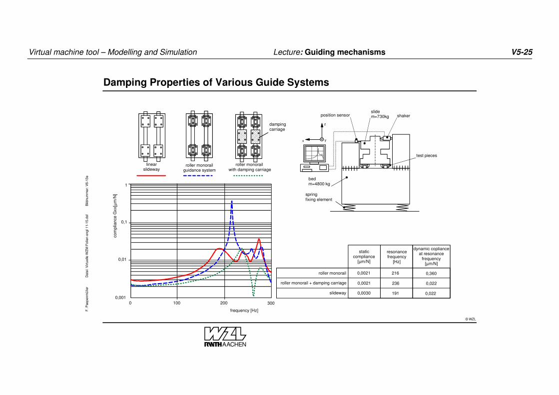
Damping properties of various guide systems

The static properties of a machine tool especially affect dimensional and form defects in the workpiece. On the other hand, dynamic problems lead to vibrations on machine, tool and workpiece, which in addition to poor surface qualities, can also cause damages to the machine and tool.

A typical bed-guide system-slide arrangement as in illustration 13 can be considered simplified as single degree of freedom system. The structure shows a massive machine bed that is supported on the foundation with metallic, soft springs in order to guarantee the neutralisation of the environment. The mounted slide corresponds to a medium size machine tool in dimensions and mass. The system is excited by an electrohydraulic relative exciter in x-direction. The acceptance of the slide displacement in x-direction is carried out by means of an inductive distance sensor.

The static and dynamic flexibility of different guide systems were determined to expose the principle-related damping properties. With comparable dimensions, the roller guide shows an approx. 30% better static stiffness than the linear sliding guide. However, the dynamic flexibility Gxx is greater by the factor 15. Generally it can be ascertained that rolling guide systems show very low damping values. Although this circumstance in multi-mass systems, e.g. machine tools, does not inevitably affect the working result negatively, in specific operating states, the low damping of the guide systems can contribute to undesirable vibrations on the workpiece. For this reason, so-called damping carriages have been developed, which run on the rails together with the rolling body carriages and which should increase the system damping through a thin oil film between damping carriages and rails (squeeze-film effect).

In illustration 13, the comparison for the roller system is shown with and without damping carriages. In the existing application, the compliance can be reduced to the level of the sliding guides. Normally, damping carriages are mounted between the rolling body carriages, so that the damping carriages likewise contribute to the stiffness in the present relaxed oscillation and shift the resonance point to higher frequencies.

However, one must remark that the use of damping carriages generally does not promise remedies for every oscillation problem. As the damping carriages are usually installed between the rolling body carriages, on corresponding excitation, their position can cover exactly with the position of an oscillation node. Then they contribute only a little or nothing at all to the reduction of the dynamic flexibility.


AACHEN

© WZL

F. P

aepe

nmül

ler

D

atei

: Virt

uelle

WZ

M F

olie

n en

gl 1

1-15

.dsf

B

ildnu

mm

er: V

6-14

ePrinciple of the Hydrodynamic Sliding Guides and Bearings

bear

ing

ga

p pr

ess

ure

p

gap length x

F

flow velocitycontour vs(y)

slide plain

slideway(slide, shaft)

movement flow

pressure flow

x

y

h(x)

dx

dyb

dimensions on aninfinitesimal

volume element

gap height

h*

pressure curve in thelubrication gap

p(x)

v

pmax

oill

oil

v

oil

v

oil

v

shaft-bearing shell

tilting blocksoil clusters in a roughened surface


Principle of the hydrodynamic sliding guides and bearings

Hydrodynamic sliding guides are particularly used in large machine tools. The components in relative motion together are separated from one another by a pressure-less supplied film of lubricant. Characteristic is that the required pressure in the lubricant gap and thus also the separation of surfaces is only generated by the relative motion. To convert the hydrodynamic principle, a wedge-shaped bearing surface is required. In sliding bearings, this arises automatically through the eccentric shaft displacement, as shown in illustration 19. If guidesways are built hydro-dynamic, surface recesses, flexible wedge elements or balance shoes must be created for the prerequisites for the hydrodynamic lubricant gap.

In illustration 19 on the right, the processes in the lubricant gap are shown. Through the motion of the track (slide, shaft, etc.), the lubricant is pushed into the lubricant gap and the liquid pressure p is developed. The speed fields vs are produced through the interference of the slip flow of the picked up liquid particles and the pressure flow, caused by the gap narrowing. To determine the characteristic size, the equilibrium of forces must be placed at a small volume element dx*dy*b (with infinite width b). Integration and consideration of the leakage losses at the sides finally deliver the carrying force F through the wedge surface:

Ψη

= pm2

0

2

Kh

bvl6F

Thereby, Kpm considers the bearing gap geometry and Ψ the leakage losses:

1h

h

0

1 − pmK

0.6 0..0235

0.7 0.0247

0.8 0.0255

0.9 0.0261

1 0.0265

1.2 0.0267

1.4 0.0265

1.5 0.0263

2.0 0.0246

b/l Ψ for 1h

h

0

1 − = 1 Ψ for 1h

h

0

1 − = 2

0.5 0.19 0.22

1.0 0.44 0.45

2.0 0.69 0.71

4.0 0.84 0.85

∞ 1.00 1.00

At a load with ∆F and differentiation, one receives the static stiffness kF:

Ψη

∆+=

pm

2

3

F

bKvl6

)FF(2k


AACHEN

© WZL

Stick-Slip Effect and Friction of Hydrodynamic Sliding GuidesF

. Pae

penm

ülle

r

Dat

ei: V

irtue

lle W

ZM

Fol

ien

engl

11-

15.d

sf

Bild

num

mer

: V6-

15e

xv

m

FZ

kF

FM

FNFR

FHaft

time t

spri

ng fo

rce

FZ

time t

slid

e p

ath

s

slidingadhesion

v*t

s

slide velocity v

fric

tion

forc

e F

R

∆v

∆FR

FR

FHaft

stick-slipregion

Stribeck curve

1 6

7

8

1

6

78

32

4

5

1

2

3

4

5

6

slideway

ball guidance system

hydrostaticguideway

GG25/ peripheral grinding

GG25/ face milling HM





GG25/ peripheral milling

GG25/ face miling HM

GG25/ face grinding

GG25/ face milling cutting ceramics

epoxy / moulding

PTFE with bronze / peripheral grinding

upper probe / machining lower probe / machining

1 2 5 10 20 50 200 500 1000 10000mm/min

fric

tion

coef

ficie

nt µ

0,15

0,1

0,05

0

A=50 * 250 mm²p=50 N/cm² upper probe

lower probe

slide oil η20=170 mPas, V=3mm³

lubrication interval ∆t=15 min

slide path s=60km

-


Stick-slip-effect and friction of hydrodynamic sliding guides

Hydrodynamic sliding guides on cutting machine tools are generally operated at medium to low speeds. In idle state, there is static friction between the sliding partners. With increasing speed, the hydrodynamic film of lubricant cannot completely separate the sliding surfaces, the guides work in the mixed friction area as shown in illustration 15. In this area, friction and wear are high, compared to higher speeds. From a specific transition speed onwards, the track floats fully and liquid friction is exclusively effective.

In the area of the mixed friction, it often gives rise to interrupted movements as a consequence of the stick-slip-effect (jerky sliding). Illustration 15 shows the causes. If an elastic force FZ with the stiffness kZ (e.g. mechanical drive components) is applied at a mass m, then firstly, the static friction must be overcome. The springs are expanded until the elastic force corresponds to the static friction to be surmounted. Thereupon, if the mass is in motion, then one must overcome only a lower mixed friction so that the slide accelerates (jerky sliding). Through that, the spring relaxes and the slide comes to a standstill. Then the static friction must be surmounted again and the cycle begins anew.

In the right illustration, the courses of the friction coefficients of various friction pairs depend on the path feed rate and surface structure. For comparison, also the friction courses of hydrostatic sliding guides and rolling guides are drawn in. It becomes clear that in hydrodynamic sliding guides and the material pairing as well as the surface structure of the sliding partners greatly affect the friction behaviour. Through peripheral grinding of both plates, a very high initial coefficient of friction and a greatly sloping curve is set, which promotes the inclination to the stick-slip effect (curve 1). Relatively uniform friction courses with increasing curve course are produced

through displaced processing structures (rails processed in guide direction, slide processed diagonal to the motion direction). For lower speeds up to 50-100 mm/min, favourable friction values and a suppression of the stick-slip-effect is defined (curves 2,3,4). Favourable friction courses show filled epoxy and PTFE (Teflon) with bronze (curve 5,6).


AACHEN

© WZL

F. P

aepe

nmül

ler

D

atei

: Virt

uelle

WZ

M F

olie

n en

gl 1

6-20

.dsf

B

ildnu

mm

er: V

6-16

eHydrostatic Sliding Guides - Fundamentals

1 pump per recess (Q=const.)

M

pT=pP

pT

F

M

pP

pT

pT

F

common pump and input restrictors(pp=konst.)

pT pT=

Q bh3

12 lη=Rt

with b refering to theunwinded land :

F

Q

h

Be Q

Q

BeLe Le Be

l

b

Le

b

l

Aeff

AR

b = Le + Be + Le + Be

= 2 ( Be + Le )

land

recess


Hydrostatic sliding guides – Fundamentals

The fundamental structure of a hydrostatic guide is shown in illustration 16, left. In one of the sliding surfaces, so-called recesses are incorporated. They are surrounded by webs of flow length l and flow width b and are provided with the oil quantity Q through supply pipes. The distance of sliding surfaces to one another is indicated as oil gap and has a height of 20 µm < h < 80 µm. The gap forms a hydraulic resistance that throttles the oil discharge from the recess and thus enables the pressure build-up, which counteracts on the outer load. The difference between the pressure in the recess and the atmospheric pressure is indicated as recess pressure pT. This pressure falls off approximately linear through the bearing web. Therefore, it can be assumed that the pressure pT is effective up to half the web width l. The effective pressure area is formed by the lengths Be and Le and is indicated as Aeff. The flow through the bearing recesses can be calculated with the help of the Hagen-Poiseuille law:

l12

bhpQ

3

Tη

= (η: dyn. viscosity)

In analogy to the Ohm’s law of electric engineering, the quotient can be defined from flow and recess pressure, and thus the hydraulic resistance RT:

3

TT

bh

l12

Q

pR

η==

Recesses with different flow lengths can be presented e.g. simply as a network of hydraulic individual resistances and calculated with the Kirchhoff’s laws for electric engineering.

The carrying capacity of a bearing recess is produced from the product of the recess pressure and the effective bearing area Aeff:

effT ApF =

To absorb eccentric loads, hydrostatic systems always require many bearing recesses. To built up different pressures in the recesses according to the equilibrium conditions, the oil supply to the recesses is independent of one another. Illustration 16 shows two possible oil supply systems.

Starting from equal supply pressure, the “1 pump per recess” system (Q=const.) has the biggest carrying capacity, as the recess pressure is only limited by the extent of the maximum pump pressure. In the “common pump and input reactors” (pP=const.), the carrying capacity is below the maximum pump pressure pP (usually 20-100 bar) depending on the design, as the total volume flow is divided and the recess pressures are uncoupled through input reactors. This system is marketed as it is economical. Different methods such as dissolving, capillary throttling, membrane throttling and current regulator can be used for uncoupling. The options vary according to costs, quality and throttle performance.

Different load-deformation relations are produced based on the arrangement, connection and throttling of bearing recesses, which are not preset at this point because of the numerous calculations.


AACHEN

© WZL

Stiffness and Damping of Hydrostatic PocketsF

. Pae

penm

ülle

r

Dat

ei: V

irtue

lle W

ZM

Fol

ien

engl

16-

20.d

sf

Bild

num

mer

: V6-

17e

0 100

25

500400300200

0

20

15

10

5

frequency [Hz]d

ampi

ng

c Öl [

Ns/

m]

h=20 µm

h=60 µmh=40 µm

0 100

60

500400300200

0

50

40

30

20

10

frequency [Hz]

stiff

ness

kÖ

l [N

/µm

]

h=20 µm

h=40 µm h=60 µm

b=45 mm

l=225 mmhQ2

Q1

h pt

y

Le

l1

l2

Be

dynamicmotion

damping coefficient

c = 2 .(Be . l2 + Le . l1 )1

h0

η

Le: effective recess legthBe: effective recess width

pt: recess pressureh0: gap heightQi: oil flow ratey: vibration directionli: land lengthη: viscosity

3 3

3

geometry of theoil gap


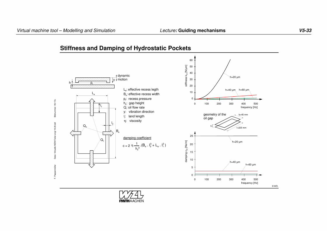
Stiffness and damping of hydrostatic recesses

Besides the stiffness, the damping based on the squeeze-film-effect is an important property of hydrostatic guides. Through the downward movement of the upper guideway surface, the oil penetrates between the web areas through the narrowing gap from outside and into the recess. Illustration 17 shows the effective width and length of the recess used for calculating the damping power. Thereby, it is assumed that a parallel flow of the length l1 and l2 is formed through the web areas. The resulting damping force is calculated by applying the Hagen Poiseuille equation and the Reynold’s differential equation. The damping coefficient c is specified as dimension for the damping of the gap. As seen from the equation for c, the initial gap must be small for high damping.

The influence of the initial gap on the important factors, dynamic stiffness and damping of an oil gap is presented in the right part of the illustration. As already mentioned in the previous observations, a lower oil gap has a positive influence on stiffness and damping through the entire excited oscillation range.


AACHEN

© WZL

F. P

aepe

nmül

ler

D

atei

: Virt

uelle

WZ

M F

olie

n en

gl 1

6-20

.dsf

B

ildnu

mm

er: V

6-18

eInfluencing variables on the guideway system

elastic deformationof the structure

size and directionof the load

preloading

roller body contact

variety and numberof the ball rows

variety of the joistconstruction (screwed)

machining andinertial forces

Fx

Fy

Fz

weight

feed forcesxy

z

F

γ

l

b

h


Influencing variables on the guideway system

While designing a rolling guided system, e.g. of a machine slide as in illustration 18, various influencing variables must be considered.

In addition to the static load through the weight of the machine table, workpiece and drive components, the feed, mass and machining forces particularly cause a dynamic load of the system. Depending on the size and orientation of the resulting forces, one or more maximum loaded guide elements are produced for a single type of burden. The design of the total system is oriented towards the dimensioning of the highest loaded guide element (carriage-rail-pair).

Rolling guide linear guides form a high-grade, overdetermined system in the mechanical sense, comprising of the non-linear stiffness performance of the rolling contacts, the flexibilities of carriers and rails as well as the connection to the ambient structure.

Only the consideration of all elasticities in a complete model enable the exact determination of the load distribution – from the complete guide through the individual guide carriages up to the rolling body itself.

The derived calculation problem can be resolved principally with the help of the Finite Element method or also analytically. The choice of the relevant method mainly depends on the problem, the required calculation and the precision.


AACHEN

© WZL

F. P

aepe

nmül

ler

D

atei

: Virt

uelle

WZ

M F

olie

n en

gl 1

6-20

.dsf

B

ildnu

mm

er: V

6-19

eNumerical Simulation of Guidance Systems

dimensioning categorylife span

staticdynamic

calculation time

level of detail

dimensioning accuracy

hardware

numerical methodFEM, BEM, MKS, analytics

guidance principleball guidance system

slideway

parameter determination for simulation and dimensioning


Numerical simulation of guidance systems

To plan and design guides and guided total systems, the most varying parameters must be considered, as shown in illustration 19. The required calculation time is the main count when simulating a system. In view of a minimum duration of the simulation, the estimation of the available calculation options is very important. Each method (analysis, finite element, boundary element, multibody simulation, etc.), the available software and the desired simulation results set certain minimum requirements on the calculation time and the modelling work. Thereby, the average calculation durations amount to a few seconds to several hours for determining simple guide system parameters, e.g. for determining the natural frequencies of entire machines or for optimisation calculations that are carried out iteratively.


AACHEN

© WZL

F. P

aepe

nmül

ler

D

atei

: Virt

uelle

WZ

M F

olie

n en

gl 1

6-20

.dsf

B

ildnu

mm

er: V

6-20

eDegree of Detailing in the Numerical Simulation

abstraction

computing time

precision

component whole model

Führungselemente


Degree of detailing in the numerical simulation

Depending on the objective of the simulation, different degrees of detailing are required for determining the targets. Therefore, before starting the modelling, it is vital to define the guide systems in order to avoid long calculation times. With increasing abstraction and simplification of the guide elements, generally, the calculating time and the calculation accuracy are reduced, illustration 20. The left illustration shows the FE model of a guide system consisting of carrier, rolling body and rails. To save calculating time, only one ‘disc’ of the system was modelled by using symmetry conditions (cutting planes x-z and y-z). Targets include the determination of stresses in the ball contact and the expansions of the guide carriages caused by the initial stress. Through accurate determination of the local pressing, the finite elements are modelled very fine in the rolling body contact.

With reduced detailing degree, firstly the rolling bodies are presented by non-linear springs and the carrier with simplified geometry. While the local deformations in the rolling contact can no longer be determined immediately, the entire deformation behaviour and the stiffness influence can be depicted through different prestresses with good accuracy.

In the last step of the abstraction, e.g. during the modelling of guide elements as part of a machine design, the total guide system is presented by a single 3-axis spring element. According to the screw joints, this is combined with the ambient design in the geometry model and provides sufficiently accurate results for the static deformation analysis as well as dynamic calculations.


AACHEN

© WZL

F. P

aepe

nmül

ler

D

atei

: Virt

uelle

WZ

M F

olie

n en

gl 2

1-25

.dsf

B

ildnu

mm

er: V

6-21

eModel Abstraction of a Rolling Guide System for FE Analysis

CAD model FE shell model with single spring elements

coordinate systemof the guidance unit

2-axes springelement

rigidelements

elementcoordinate system

1

1

2

2

3

3

4

4

5

5

6

6

7

7

8

8

coordinate systemof the guidance unit

2-axis springelements

FE shell model with one spring element and rigid elements


Model abstraction of a rolling guide system for the FE analysis

In illustration 21, the geometry model and the FE spring model of a profile rail guide system are compared. The connection designs of machine table and frame are approximated in the FE model through shell elements with a specific theoretical thickness.

In the upper FE model, the relevant node pairs with a spring element each are connected in the position of the guide carriage, shown in grey in the illustration. In this case, the total stiffness of a guide carriage must be distributed on the eight spring elements. Two stiffnesses (lateral and tension/compression) are assigned to each spring element for the rail direction. The disadvantage in this modelling is that the nodes of the spring elements are placed away from each other. When loading the guide carriages normal to the rail direction, the upper connecting nodes of the springs are displaced, so that the direction of the spring axes changes. Depending on the arrangement of springs and the extent of displacement, faults can arise here during the calculation.

In the lower FE model, the connections of the rails and the guide carriage are guided to a central node each. The connection is provided through ideal rigid rods. The two central nodes are combined with a single two-axis spring, which represent the stiffnesses of the guide system in tension/compressionand lateral direction. In the last step, the nodes are pushed together in one point. Displacements of the spring axes, like in the above design are thus avoided.

Possible stiffening in the design through the profile rails and the damping values are not considered in this modelling. In this modelling, one must note that the nodes of the individual springs run on one axis each and the axes run exactly parallel to one another.

Thus the initiation of effective forces with false stiffness ratios in the design and a falsified deformation of the total model are avoided.


AACHEN

© WZL

F. P

aepe

nmül

ler

D

atei

: Virt

uelle

WZ

M F

olie

n en

gl 2

1-25

.dsf

B

ildnu

mm

er: V

6-22

eFE Model of a Traverse Column with Linear Guide Systems

rigid connection of thecolumn to the environment

xz

y

3 axes spring elementrepresenting the drive(kx,kz << ky)

3 axes spring elementrepresenting the guidancesystem(kx,kz >> ky)


FE model of a traverse column with linear guide systems

Illustration 22 shows the FE model of a machine tool boring mill with simplified drive and guide elements. The sheet thickness is identified by the different coloured shell elements. Because in this case only the deformations of the column should be ascertained (and not those of the entire machine), ideally it is combined fixed with the environment in the floor area in the position of the x-axis guide elements.

The guide rails of the y-axis run vertical to the shell elements and are not shown. In position of the y-guide carriage, rigid rod elements (rigids) are star-shaped combined with the yellow connecting area. They have the task of copying the joint points of the guide carriage on the real column and to initiate the forces at these points. In the star point of the rigid elements, a three-axis spring element is connected, which preserves the stiffness values of a guide carriage. The stiffness in traverse direction (y) is set to zero. The required stiffness in y-direction is converted by the modelling of the mechanical drive (here ball roller spindle). While, with almost same modelling strategy, the stiffnesses are normally set against zero for the traverse direction, the drive stiffness is specified in y-direction.



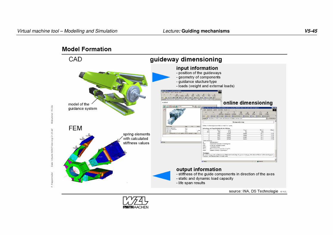
Model formation

Illustration 23 shows the method for model formation with the example of a milling head design. The movement in z-direction is realised through three slide units that are moved on 4 rolling guide carriages each.

After determining the geometric dimensions of components in the CAD system, suitable guide systems are selected with the help of analytical calculation tools, some of which are available on the Internet. The knowledge of the following input quantities is required:

- Geometry of components (bed, slide, column)

- Position of guide elements

- Selection of a suitable style of guide

- Load collective (masses, forces, moments, speeds)

With the calculation programs, one can determine the maximum loaded guide elements for the specified load cycle and the following output quantities:

- Dynamic carrying capacities of the guide elements

- Carrying safeties

- Life span

- Displacements of the axis (slides, columns)

- Displacements of the points of application of force (tool)

With the help of the calculation results, the ‘position of guide elements’ and ‘guide model’ input parameters can be easily modified and matched to an optimum result.

The displacements ascertained in dependence of the load collective can be converted to stiffness values for the axis directions and accepted as big value for the FE spring elements.

With the data acquired in such a way, the static and dynamic behaviour of the milling head design can be examined and optimised.


AACHEN

© WZL

F. P

aepe

nmül

ler

D

atei

: Virt

uelle

WZ

M F

olie

n en

gl 2

1-25

.dsf

B

ildnu

mm

er: V

6-24

eAnalytical Calculation Methods of Rolling Guide Systems 1

linear method according to DIN 636

basic load capacitymomentslife span

- for centric load direction- insufficient statements on spatial loads

non-linear method (elastic roller bodies)

basic load capacitymomentsdeformations of the roller bodieslife spanclearance/preloadingpath tiltpressure angle displacements of balls

- for eccentric load direction- inner load distribution on the roller bodies- roller body deflection- displacement of the point of application of load- no consideration of the elastic joint construction

enhanced non-linear method (fully elastic model)

- for eccentric load direction- inner load distribution on the roller bodies- roller body deflection- displacement of the point of application of load- consideration of the elastic joint construction (influence numbers determined by FEA)

basic load capacitymomentsdeformation of the whole system life spanclearance/preloadingpath tiltpressure angle displacements of balls

source: INA


Analytic calculation method of rolling guide systems 1

While calculating the properties of rolling guides, different calculation methods are used, which differ from each other considerably in the model acceptance and results, illustration 24.

a) The preset DIN capacity definitions for rolling guides apply for centric acting load directions. To consider the spatial load cases prevalent in practice, normally one refers to the details of the guide manufacturer. However, a statement on the inner load distribution in the rolling guides is not possible.

b) The non-linear method permits the consideration of eccentric acting load directions. The ambient design and the bearing parts must be rigid. In analogy to the classical calculation of rotating rolling bearings, which consider only the contact deformation rolling body-track, these methods can also be applied for linear bearing. Thereby, the state of equilibrium between the specified outer load and the inner load distribution is determined.

)n...1j,5...1i(qTbn

1j

jiji ===∑=

(1)

bi: Components of outer system load

Tij: Components of transformation matrix

qj: Rolling body forces

n: Number of rolling bodies

i: Number of variants

The spring deflections of the rolling bodies can be calculated from the displacements of the rigid components vis-à-vis the foundation

through simple geometric considerations. The rolling body load is produced from the non-linear spring equation

Q

Rj Cq/1δ= (2)

CR: Rolling body spring value dependent on material properties and the geometry

δi: Total elastic deformation at both contact points of the rolling body

Q: Exponent for point / linear contact

The subsequent geometric summation of the rolling body forces at the point of the load initiation produces the applied load. The non-linear equation system given through (1) and (2), is resolved iteratively. This method provides adequately accurate results for a number of guide systems.

Life reducing influences such as tolerance, prestress and track tipping and contact angle change are considered.

c) If the traditional non-linear method is not enough, i.e. the elasticities of the environment design have a decisive influence on the total behaviour, an extension of the calculation method is required. The influence of additional flexibilities on life and load distribution of specific rolling guide carriages can be decisive for the total behaviour. The extended method is based on calculation fundamentals for rotary bearing on the basis of the theory of the highly curved beam for the housing deformations.


AACHEN

© WZL

F. P

aepe

nmül

ler

D

atei

: Virt

uelle

WZ

M F

olie

n en

gl 2

1-25

.dsf

B

ildnu

mm

er: V

6-25

e

source: INA

Analytical Calculation Methods of Rolling Guide Systems 2

Fy

Mz

Mx

componentload

withoutpreloading

preloading10% of C

withoutpreloading

preloading10% of C

withoutpreloading

preloading10% of C

linear method (DIN) non-linear method enhanced non-linear method

loading of the maximum loaded components of the guidance system

FyE [N]

FzE [N]

MxE [Nm]

MzE [Nm]

MyE [Nm]

FyE [N]

FzE [N]

MxE [Nm]

MzE [Nm]

MyE [Nm]

FyE [N]

FzE [N]

MxE [Nm]

MzE [Nm]

MyE [Nm]

12500

-

-

-

-

12500

-

-

-

-

12500

-

-

-

-

12500

-

-

-

-

12500

-

-

-

-

12500

-

-

-

-

12500

-

-

-

-

12104

2357

37

-

-

11385

-

-

100

-

12500

-

-

-

-

12173

270

30

-

-

11560

-

-

85

-

12500

-

-

-

-

12214

315

31

-

-

10707

-

-

183

-

12500

-

-

-

-

12126

2133

35

-

-

10441

-

-

186

-


Analytic calculation method of rolling guide systems 2

By means of influencing values, the housing deformations are considered while determining the state of equilibrium of the bearing. With the equations (1) and (2), the non-linear equation system to be resolved is given. The flexibilities of the environment design reduce the rolling body elasticities by the factor of the influencing values:

jjj w−= 0δδ (3), with

∑=

=n

1k

kjkj qCw (4)

wj: Total deformation of carrier and rails at the point j as a result of n roller body forces

Cjk: Influencing value at the point j as a result of the load at the point k

The inner non-linear equation system with the unknown displacements δ1,δ2,...,δn is produced from (3).

∑=

δ+δ−δ=n

1j

Q/1

jRj10111 CCf

∑=

δ+δ−δ=n

1j

Q/1

jRj20222 CCf (5)

∑=

δ+δ−δ=n

1j

Q/1

jRnjn0nn CCf

The system is not resolvable completely, so that starting from the estimated solution δj

(0) and solution of the linear equation system

( )∑=

+ =δ−δδ∂

∂+

n

1j

)m(

j

)1m(

j

j

i

i 0f

f (i,j=1,2,...,n) (6)

one can determine solutions δj(m+1). The determinants result from:

jifürCCQ/1f 1Q/1

jRij

j

i ≠δ=δ∂

∂ − (7)

jifürCCQ/11f 1Q/1

jRij

j

i =δ+=δ∂

∂ − (8)

The corrections δj(m+1) ascertained with (6) are again the starting point

for the following approximation solution. The error correction is carried out until the central quadratic error fm is less than a selected limit ε.

The influencing values Cjk can be completely calculated due to the complex rail and carrier geometry and are therefore ascertained with the FE method.

Illustration 25 shows the comparison of the calculation method default here in the example of a profile rail rolling guide with rollers. Individual loads were selected as system loads: Fy=50kN, Mx=4625Nm and Mz=4500Nm. The results are presented for the maximum loaded guide element respectively. The calculation results vary by up to 15%. But more vital is that realistic states, such as the system prestress or the guide carriage tipping, cannot be acquired with the linear method. For example, with the prestress of 0.1C, rolling body load increases by up to 35 at a system load of 50 kN.


© WZL

F. P

aepe

nmül

ler

D

atei

: Virt

uelle

WZ

M F

olie

n en

gl 2

6-29

.dsf

B

ildnu

mm

er: V

6-26

eLife Span Comparison on the Basis of the Calculation Methods

source: INA

linear method non-linear method enhanced non-linear method

0% 5% 10%preloading of C

Fy


Mx


Mz

AACHEN


Life span comparison on the basis of the calculation methods

Besides the prestress, even the inner load distribution and subsequently even the rolling body maximum load is greatly influenced by the tipping of the elements. Moments Mx at the traverse axis, as seen in illustration 26, cause a high edge load of the rolling body. Together with a prestress of 0.1C, the loads increase by 50% as opposed to a untipped, non-prestressed roller, as they would have been calculated with the linear method.

Moments Mz at the lateral axis, as they occur during acceleration and braking, act on the static and dynamic carrying capacity. In turn, the rolling body loads increase by up to 180% as compared to the linear method, mainly caused by the elastic deformations of rail and carrier.

The results clarify that same results can be obtained with the different methods for pure tension/compressionloads (Fy) of non-prestressed guide systems. In initial state, prestressed elements are essentially loaded higher than can even be calculated with the linear method. If moments also affect the guides, it is not permitted to reduce the load absorption of the guide carriage to a point and to subsequently neglect the reaction moments. The effects of the moments considered in addition, on the life is shown in illustration 26. System prestress and load moments here cause a decrease of the life to 30% of the values determined with the linear method.


AACHEN

© WZL

F. P

aepe

nmül

ler

D

atei

: Virt

uelle

WZ

M F

olie

n en

gl 2

6-29

.dsf

B

ildnu

mm

er: V

6-27

eFE Model Formation to Calculate Sliding Guides

z

x

y

1' 2'

3' 4'

5' 6'

7'8'

1''

2''

3'' 4''

5''

6''

7''8''

1*

2*3*

4*

1°

2°

machine slide FE model using beam elements

l

joint i

Fzi

FyizMi

Fxi

xMi

yMi

Fz

Fx

xMzM

yM Fy

i+1

i+1

i+1

i+1

i+1i+1

joint i+1beam element for3-dimensional structures

guideway path

joint

beam element front table geometry

beam element rear table geometry

beam element connection

beam element guideway

beam element force application


FE model formation to calculate the sliding guides

Due to the guide flexibility, the calculation of the static displacement behaviour of slide designs with sliding guides leads to multiple static over-defined systems arranged in any way, which cannot be resolved with traditional calculation approaches. A possible solution is the application of the Finite Element Method (FEM). With it, the displacements of all geometry points existing in the system and the guide element and load contact points can be calculated. By using various finite elements, guide elements of any position, contact points and stiffness behaviour can be considered. Through iterative solution methods, it is possible to calculate non-linear stiffness courses of guide systems.

As seen in illustration 27, the calculation model required for the FEM is composed of beam elements, which lie between two nodes respectively. The nodes lie in the corner points of the geometry, and in the guide contact point and point of application of force.

For static analysis, the component to be examined with the help of easy to describe beam elements are discretised. During the formulation of the static behaviour (matrix stiffness method), a linear equation system is developed, whose independent variables correspond to the degrees of freedom of the structure to be considered.

[ K ] ⋅ { u } = { F }

[ K ]: Stiffness matrix,

{ u }: Displacement vector,

{ F }: Outer loads.

The displacement is obtained by solving the equation system according to the displacement vector.

To create the stiffness matrix, the structure to be calculated is divided into individual segments (finite elements), which are combined with one another through nodes. For these elements, an element stiffness matrix is placed by considering thrust, pressure, bend and torsion, wherein the stiffness properties of the element are reduced to both corner nodes.

While calculating the three-dimensional components, e.g. guide slides, beam elements with six degrees of freedom are required (illustration 27). According to the six degrees of freedom per node, a 12 x 12 matrix is produced for a beam element.


AACHEN

© WZL

F. P

aepe

nmül

ler

D

atei

: Virt

uelle

WZ

M F

olie

n en

gl 2

6-29

.dsf

B

ildnu

mm

er: V

6-28

eStiffness Matrix of a 3-dimensional Model Using Beam Elements

E11 2 3 4

5

E2 E3 E4 LO

E1E2

E3

E3E4

E4

E4LO

E1 E1

E1E2

E2E2

E2E3

E2E3

E3

E3E4

E4

E4LO

joint number

1

1

2

2

degree of freedom

5

3

4

5 symmetrical

zeroE1 E1

band widthband width

12 3456

123456

789101112

789

101112....


Stiffness matrix of a three-dimensional beam model

The stiffness matrix of a complete structure is gained through superposition of the element matrices. In illustration 28, this method is shown as example for the stiffness matrix of a five-node beam model, comprising of 4 elements with the markings E1 to E4.

The therms of the element stiffness matrices are entered in the total stiffness matrix according to their node numbering. In addition, at the node 5, the properties of the chucking (bearing 0) are superimposed. The total stiffness matrix is built symmetric to the main diagonals. Besides, it also shows a clear band structure, which means that the matrix is occupied only in one narrow band parallel to the main diagonals. The width of this band is indicated as bandwidth and is shown in example 12.

The guide elements lying one behind the other on a track in y-direction, are considered as spring elements, whereby the stiffness can be defined from the stiffness characteristic lines calculated or measured for each track. In case of guideways, which can be loaded in carrying and transverse direction, a carrying element is composed of two springs. Thereby, one spring is in the track direction and the other vertical to the track direction.

For the FE calculation, all values must be related to a common coordinate system. If a track is not parallel to the global coordinates, the scalar stiffness values are referred to the global coordinate system by means of the coordinate transformation.

The determination of the track displacement at outer load cannot be carried out completely, as almost all guide principles show a non-linear stiffness behaviour. Therefore, one starts from an initial stiffness of the loaded track. This is either produced from the entered initial load or from the initial gap. With the help of this initial stiffness,

a primary displacement can be ascertained by charging the outer load by means of the finite element calculation. The solution of the equation system is then carried out iteratively with a selectable number of iteration steps.


AACHEN

© WZL

F. P

aepe

nmül

ler

D

atei

: Virt

uelle

WZ

M F

olie

n en

gl 2

6-29

.dsf

B

ildnu

mm

er: V

6-29

eCalculation of Hydrodynamic and Hydrostatic Guides

input parameters

geometry

loads

- mass

- forces/moments

- drive

raceway position

mating of material

surface roughness

results

displacements

- guideways

- points of force

application

guideway stiffness

reaction forces

displacement animation


Calculation of hydrodynamic and hydrostatic guides

Illustration 29 shows a program interface for calculating hydrodynamic and hydrostatic guides on machine slides. The software works according to the Finite Element method described above.

In addition to defining the geometry data and the points of application of force, the user can select various slideway plates or oil supply systems. The generation of the beam model, the required transformations and the solution of the equation system is automatic.

After completing the calculations, the user receives information on the force ratios in the tracks, possible overstress, displacements of tracks and the point of application of force, as well as the reactive forces defined in the guides.

In addition, through animation of the slide displacement, the effects of the acting forces are displayed.

Documents

Lecture 5: Guiding mechanisms - RWTH Aachen … machine tool ... Quasi-static study of a ... optimisation of the guide systems with regard to the stiffness, the static and dynamic