Lecture 5:Basic Dynamical Systems

CS 344R: Robotics

Benjamin Kuipers

Dynamical Systems• A dynamical system changes continuously

(almost always) according to

• A controller is defined to change the coupled robot and environment into a desired dynamical system.

€

˙ x =F(x) where x∈ℜn

€

˙ x = F(x,u)

y = G(x)

u = H i(y)

€

˙ x = F(x,H i(G(x)))

In One Dimension

• Simple linear system

• Fixed point

• Solution

– Stable if k < 0

– Unstable if k > 0

€

˙ x =kx

€

x =0 ⇒ ˙ x =0

€

x

€

˙ x

€

x(t)=x0 ekt

In Two Dimensions

• Often, position and velocity:

• If actions are forces, causing acceleration:

€

x=(x,v)T where v=˙ x

€

˙ x =˙ x ˙ v

⎛

⎝ ⎜ ⎜

⎞

⎠ ⎟ ⎟ =

˙ x ˙ ̇ x

⎛

⎝ ⎜ ⎜

⎞

⎠ ⎟ ⎟ =

v

forces

⎛

⎝ ⎜ ⎜

⎞

⎠ ⎟ ⎟

€

The Damped Spring

• The spring is defined by Hooke’s Law:

• Include damping friction

• Rearrange and redefine constants

xkxmmaF 1−=== &&

xkxkxm &&& 21 −−=

0=++ cxxbx &&&

€

˙ x =˙ x ˙ v

⎛

⎝ ⎜ ⎜

⎞

⎠ ⎟ ⎟ =

˙ x ˙ ̇ x

⎛

⎝ ⎜ ⎜

⎞

⎠ ⎟ ⎟ =

v

−b˙ x −cx

⎛

⎝ ⎜ ⎜

⎞

⎠ ⎟ ⎟

The Linear Spring Model

• Solutions are:

• Where r1, r2 are roots of the characteristic equation

€

˙ ̇ x +b˙ x +cx=0

€

λ2 +bλ +c =0

€

r1,r2 =−b± b2 −4c

2

€

x(t)=Aer1t +Ber2t

€

c ≠ 0

Qualitative Behaviors

• Re(r1), Re(r2) < 0 means stable.

• Re(r1), Re(r2) > 0 means unstable.

• b2-4c < 0 means complex roots, means oscillations.

b

cunstable stable

spiral

nodalnodal

unstable

€

r1,r2 =−b± b2 −4c

2

Generalize to Higher Dimensions

• The characteristic equation for generalizes to – This means that there is a vector v such that

• The solutions are called eigenvalues.

• The related vectors v are eigenvectors.

€

˙ x =Ax

€

det(A−λI )=0

€

Av=λv

€

λ

Qualitative Behavior, Again

• For a dynamical system to be stable:– The real parts of all eigenvalues must be negative.– All eigenvalues lie in the left half complex plane.

• Terminology:– Underdamped = spiral (some complex eigenvalue)– Overdamped = nodal (all eigenvalues real)– Critically damped = the boundary between.

Node Behavior

Focus Behavior

Saddle Behavior

Spiral Behavior

(stable attractor)

Center Behavior

(undamped oscillator)

The Wall Follower

(x,y)

€

θ

The Wall Follower• Our robot model:

u = (v )T y=(y )T 0.

• We set the control law u = (v )T = Hi(y)

€

˙ x =

˙ x ˙ y ˙ θ

⎛

⎝

⎜ ⎜ ⎜

⎞

⎠

⎟ ⎟ ⎟ =F (x,u) =

vcosθ

vsinθ

ω

⎛

⎝

⎜ ⎜ ⎜

⎞

⎠

⎟ ⎟ ⎟

€

e=y−yset so ˙ e =˙ y and ˙ ̇ e =˙ ̇ y

The Wall Follower

• Assume constant forward velocity v = v0

– approximately parallel to the wall: 0.

• Desired distance from wall defines error:

• We set the control law u = (v )T = Hi(y)

– We want e to act like a “damped spring”

€

e=y−yset so ˙ e =˙ y and ˙ ̇ e =˙ ̇ y

€

˙ ̇ e +k1 ˙ e +k2 e=0

The Wall Follower

• We want

• For small values of

• Assume v=v0 is constant. Solve for

– This makes the wall-follower a PD controller.

€

˙ ̇ e +k1 ˙ e +k2 e=0

€

˙ e = ˙ y = vsinθ ≈ vθ˙ ̇ e = ˙ ̇ y = vcosθ ˙ θ ≈ vω

€

u =v

ω

⎛

⎝ ⎜

⎞

⎠ ⎟=

v0

−k1θ −k2

v0

e

⎛

⎝

⎜ ⎜

⎞

⎠

⎟ ⎟= H i(e,θ)

Tuning the Wall Follower

• The system is

• Critically damped is

• Slightly underdamped performs better.– Set k2 by experience.

– Set k1 a bit less than

€

˙ ̇ e +k1 ˙ e +k2 e=0

€

k12 −4k2 =0

€

k1 = 4k2

€

4k2

An Observer for Distance to Wall

• Short sonar returns are reliable.– They are likely to be perpendicular reflections.

Experiment with Alternatives

• The wall follower is a PD control law.

• A target seeker should probably be a PI control law, to adapt to motion.

• Try different tuning values for parameters.– This is a simple model.– Unmodeled effects might be significant.

Ziegler-Nichols Tuning

• Open-loop response to a step increase.

d T K

Ziegler-Nichols Parameters

• K is the process gain.

• T is the process time constant.

• d is the deadtime.

Tuning the PID Controller

• We have described it as:

• Another standard form is:

• Ziegler-Nichols says:

€

u(t) =−kP e(t)−kI edt0

t

∫ −kD ˙ e (t)

€

u(t) = −P e(t) + TI e dt0

t

∫ + TD ˙ e (t) ⎡

⎣ ⎢

⎤

⎦ ⎥

€

P =1.5 ⋅TK ⋅d

TI = 2.5 ⋅d TD = 0.4 ⋅d

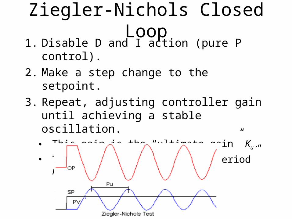
Ziegler-Nichols Closed Loop1. Disable D and I action (pure P control).

2. Make a step change to the setpoint.

3. Repeat, adjusting controller gain until achieving a stable oscillation.

• This gain is the “ultimate gain” Ku.

• The period is the “ultimate period” Pu.

Closed-Loop Z-N PID Tuning

• A standard form of PID is:

• For a PI controller:

• For a PID controller:

€

u(t) = −P e(t) + TI e dt0

t

∫ + TD ˙ e (t) ⎡

⎣ ⎢

⎤

⎦ ⎥

€

P = 0.45 ⋅Ku TI =Pu

1.2

€

P = 0.6 ⋅Ku TI =Pu

2TD =

Pu

8