Embed Size (px)
Citation preview
Lecture 4: Term Weighting and the Vector Space
ModelInformation Retrieval
Computer Science Tripos Part II
Simone Teufel
Natural Language and Information Processing (NLIP) Group
Lent 2014
147

IR System Components
IR SystemQuery
Document
Collection
Set of relevant
documents
Document Normalisation
Indexer
UI
Ranking/Matching ModuleQuery
Norm
.
Indexes
Today: The ranker/matcher
148

IR System Components
IR SystemQuery
Document
Collection
Set of relevant
documents
Document Normalisation
Indexer
UI
Ranking/Matching ModuleQuery
Norm
.
Indexes
Finished with indexing, query normalisation
149
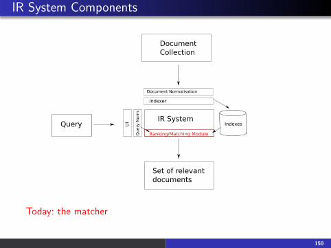
IR System Components
IR SystemQuery
Document
Collection
Set of relevant
documents
Document Normalisation
Indexer
UI
Ranking/Matching ModuleQuery
Norm
.
Indexes
Today: the matcher
150

Overview
1 Recap
2 Why ranked retrieval?
3 Term frequency
4 Zipf’s Law and tf-idf weighting
5 The vector space model
151
Overview
1 Recap
2 Why ranked retrieval?
3 Term frequency
4 Zipf’s Law and tf-idf weighting
5 The vector space model

Recap: Tolerant Retrieval
What to do when there is no exact match between query termand document term?
Dictionary as hash, B-trie, trie
Wildcards via permuterm
and k-gram index
k-gram index and edit-distance for spelling correction
152

Recap: Large-scale, distributed indexing
BSBI and SPIMI
MapReduce
Reuters RVC1 and Heap’s Law
153
Upcoming
Ranking search results: why it is important (as opposed tojust presenting a set of unordered Boolean results)
Term frequency: This is a key ingredient for ranking.
Tf-idf ranking: best known traditional ranking scheme
And one explanation for why it works: Zipf’s Law
Vector space model: One of the most important formalmodels for information retrieval (along with Boolean andprobabilistic models)
154

Overview
1 Recap
2 Why ranked retrieval?
3 Term frequency
4 Zipf’s Law and tf-idf weighting
5 The vector space model
Ranked retrieval
Thus far, our queries have been Boolean.
Documents either match or don’t.
Good for expert users with precise understanding of theirneeds and of the collection.
Also good for applications: Applications can easily consume1000s of results.
Not good for the majority of users
Don’t want to write Boolean queries or wade through 1000sof results.
This is particularly true of web search.
155
Problem with Boolean search: Feast or famine
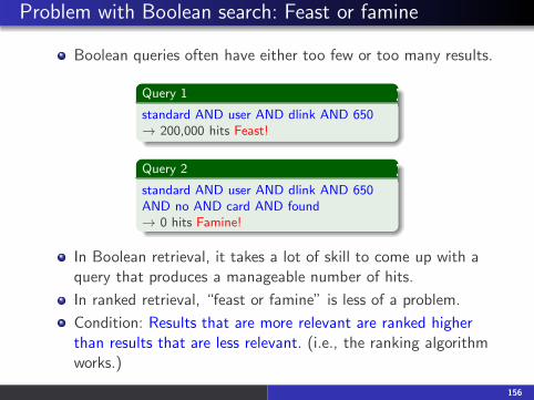
Boolean queries often have either too few or too many results.
Query 1
standard AND user AND dlink AND 650
→ 200,000 hits Feast!
Query 2
standard AND user AND dlink AND 650
AND no AND card AND found
→ 0 hits Famine!
In Boolean retrieval, it takes a lot of skill to come up with aquery that produces a manageable number of hits.
In ranked retrieval, “feast or famine” is less of a problem.
Condition: Results that are more relevant are ranked higherthan results that are less relevant. (i.e., the ranking algorithmworks.)
156
Scoring as the basis of ranked retrieval
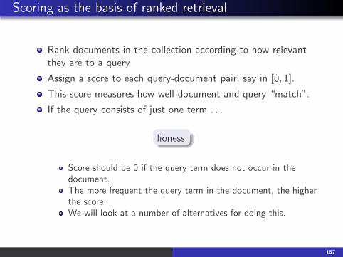
Rank documents in the collection according to how relevantthey are to a query
Assign a score to each query-document pair, say in [0, 1].
This score measures how well document and query “match”.
If the query consists of just one term . . .
lioness
Score should be 0 if the query term does not occur in thedocument.The more frequent the query term in the document, the higherthe scoreWe will look at a number of alternatives for doing this.
157

Take 1: Jaccard coefficient
A commonly used measure of overlap of two sets
Let A and B be two sets
Jaccard coefficient:
jaccard(A,B) =|A ∩ B ||A ∪ B |
(A 6= ∅ or B 6= ∅)jaccard(A,A) = 1
jaccard(A,B) = 0 if A ∩ B = 0
A and B don’t have to be the same size.
Always assigns a number between 0 and 1.
158

Jaccard coefficient: Example
What is the query-document match score that the Jaccardcoefficient computes for:
Query
“ides of March”
Document
“Caesar died in March”
jaccard(q, d) = 1/6
159

What’s wrong with Jaccard?
It doesn’t consider term frequency (how many occurrences aterm has).
Rare terms are more informative than frequent terms.Jaccard does not consider this information.
We need a more sophisticated way of normalizing for thelength of a document.
Later in this lecture, we’ll use |A ∩ B|/√
|A ∪ B| (cosine) . . .. . . instead of |A ∩ B|/|A ∪ B| (Jaccard) for lengthnormalization.
160

Overview
1 Recap
2 Why ranked retrieval?
3 Term frequency
4 Zipf’s Law and tf-idf weighting
5 The vector space model

Binary incidence matrix
Anthony Julius The Hamlet Othello Macbeth . . .and Caesar Tempest
CleopatraAnthony 1 1 0 0 0 1Brutus 1 1 0 1 0 0Caesar 1 1 0 1 1 1Calpurnia 0 1 0 0 0 0Cleopatra 1 0 0 0 0 0mercy 1 0 1 1 1 1worser 1 0 1 1 1 0. . .
Each document is represented as a binary vector ∈ {0, 1}|V |.
161
Count matrix
Anthony Julius The Hamlet Othello Macbeth . . .and Caesar Tempest
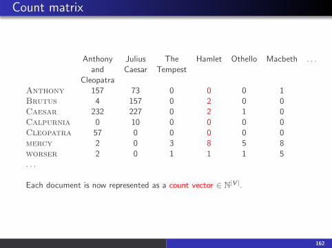
CleopatraAnthony 157 73 0 0 0 1Brutus 4 157 0 2 0 0Caesar 232 227 0 2 1 0Calpurnia 0 10 0 0 0 0Cleopatra 57 0 0 0 0 0mercy 2 0 3 8 5 8worser 2 0 1 1 1 5. . .
Each document is now represented as a count vector ∈ N|V |.
162

Bag of words model
We do not consider the order of words in a document.
Represented the same way:
John is quicker than MaryMary is quicker than John
This is called a bag of words model.
In a sense, this is a step back: The positional index was ableto distinguish these two documents.
We will look at “recovering” positional information later inthis course.
For now: bag of words model
163
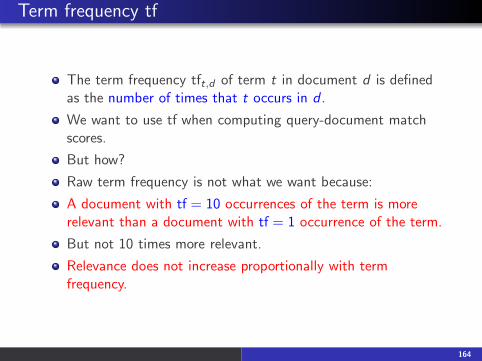
Term frequency tf
The term frequency tft,d of term t in document d is definedas the number of times that t occurs in d .
We want to use tf when computing query-document matchscores.
But how?
Raw term frequency is not what we want because:
A document with tf = 10 occurrences of the term is morerelevant than a document with tf = 1 occurrence of the term.
But not 10 times more relevant.
Relevance does not increase proportionally with termfrequency.
164
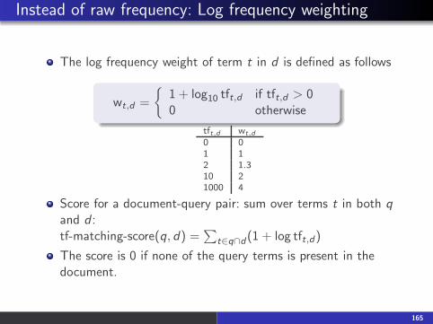
Instead of raw frequency: Log frequency weighting
The log frequency weight of term t in d is defined as follows
wt,d =
{
1 + log10 tft,d if tft,d > 00 otherwise
tft,d wt,d
0 01 12 1.310 21000 4
Score for a document-query pair: sum over terms t in both qand d :tf-matching-score(q, d) =
∑
t∈q∩d (1 + log tft,d)
The score is 0 if none of the query terms is present in thedocument.
165

Overview
1 Recap
2 Why ranked retrieval?
3 Term frequency
4 Zipf’s Law and tf-idf weighting
5 The vector space model

Frequency in document vs. frequency in collection
In addition, to term frequency (the frequency of the term inthe document) . . .
. . . we also want to use the frequency of the term in thecollection for weighting and ranking.
Now: excursion to an important statistical observation aboutlanguage.
166

Zipf’s law
How many frequent vs. infrequent terms should we expect ina collection?
In natural language, there are a few very frequent terms andvery many very rare terms.
Zipf’s law
The i th most frequent term hasfrequency cfi proportional to 1/i :
cfi ∝ 1i
cfi is collection frequency: the number of occurrences of theterm ti in the collection.
167
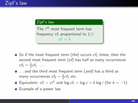
Zipf’s law
Zipf’s law
The i th most frequent term hasfrequency cfi proportional to 1/i :
cfi ∝ 1i
So if the most frequent term (the) occurs cf1 times, then thesecond most frequent term (of) has half as many occurrencescf2 =
12cf1 . . .
. . . and the third most frequent term (and) has a third asmany occurrences cf3 =
13cf1 etc.
Equivalent: cfi = cik and log cfi = log c + k log i (for k = −1)
Example of a power law
168

Zipf’s Law: Examples from 5 Languages
Top 10 most frequent words in a large language sample:
English German Spanish Italian Dutch
1 the 61,847 1 der 7,377,879 1 que 32,894 1 non 25,757 1 de 4,7702 of 29,391 2 die 7,036,092 2 de 32,116 2 di 22,868 2 en 2,7093 and 26,817 3 und 4,813,169 3 no 29,897 3 che 22,738 3 het/’t 2,4694 a 21,626 4 in 3,768,565 4 a 22,313 4 e 18,624 4 van 2,2595 in 18,214 5 den 2,717,150 5 la 21,127 5 e 17,600 5 ik 1,9996 to 16,284 6 von 2,250,642 6 el 18,112 6 la 16,404 6 te 1,9357 it 10,875 7 zu 1,992,268 7 es 16,620 7 il 14,765 7 dat 1,8758 is 9,982 8 das 1,983,589 8 y 15,743 8 un 14,460 8 die 1,8079 to 9,343 9 mit 1,878,243 9 en 15,303 9 a 13,915 9 in 1,63910 was 9,236 10 sich 1,680,106 10 lo 14,010 10 per 10,501 10 een 1,637
169

Zipf’s law: Rank × Frequency ∼ Constant
English: Rank R Word Frequency f R × f
10 he 877 8770
20 but 410 8200
30 be 294 8820
800 friends 10 8000
1000 family 8 8000
German: Rank R Word Frequency f R × f
10 sich 1,680,106 16,801,060
100 immer 197,502 19,750,200
500 Mio 36,116 18,059,500
1,000 Medien 19,041 19,041,000
5,000 Miete 3,755 19,041,000
10,000 vorlaufige 1.664 16,640,000
170
Other collections (allegedly) obeying power laws
Sizes of settlements
Frequency of access to web pages
Income distributions amongst top earning 3% individuals
Korean family names
Size of earth quakes
Word senses per word
Notes in musical performances
. . .
171

Zipf’s law for Reuters
0 1 2 3 4 5 6 7
01
23
45
67
log10 rank
log1
0 cf
Fit is not great. Whatis important is thekey insight: Few fre-quent terms, manyrare terms.
172
Desired weight for rare terms
Rare terms are more informative than frequent terms.
Consider a term in the query that is rare in the collection(e.g., arachnocentric).
A document containing this term is very likely to be relevant.
→ We want high weights for rare terms likearachnocentric.
173
Desired weight for frequent terms
Frequent terms are less informative than rare terms.
Consider a term in the query that is frequent in the collection(e.g., good, increase, line).
A document containing this term is more likely to be relevantthan a document that doesn’t . . .
. . . but words like good, increase and line are not sureindicators of relevance.
→ For frequent terms like good, increase, and line, wewant positive weights . . .
. . . but lower weights than for rare terms.
174
Document frequency
We want high weights for rare terms like arachnocentric.
We want low (positive) weights for frequent words like good,increase, and line.
We will use document frequency to factor this into computingthe matching score.
The document frequency is the number of documents in thecollection that the term occurs in.
175

idf weight
dft is the document frequency, the number of documents thatt occurs in.
dft is an inverse measure of the informativeness of term t.
We define the idf weight of term t as follows:
idf weight
idft = log10N
dft
(N is the number of documents in the collection.)
idft is a measure of the informativeness of the term.
log N
dftinstead of N
dftto “dampen” the effect of idf
Note that we use the log transformation for both termfrequency and document frequency.
176

Examples for idf
Compute idft using the formula: idft = log101,000,000
dft
term dft idftcalpurnia 1 6animal 100 4sunday 1000 3fly 10,000 2under 100,000 1the 1,000,000 0
177

Effect of idf on ranking
idf affects the ranking of documents for queries with at leasttwo terms.
For example, in the query “arachnocentric line”, idf weightingincreases the relative weight of arachnocentric anddecreases the relative weight of line.
idf has little effect on ranking for one-term queries.
178

Collection frequency vs. Document frequency
Collection DocumentTerm frequency frequencyinsurance 10440 3997try 10422 8760
Collection frequency of t: number of tokens of t in thecollection
Document frequency of t: number of documents t occurs in
Clearly, insurance is a more discriminating search term andshould get a higher weight.
This example suggests that df (and idf) is better for weightingthan cf (and “icf”).
179
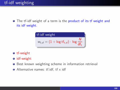
tf-idf weighting
The tf-idf weight of a term is the product of its tf weight andits idf weight.
tf-idf weight
wt,d = (1 + log tft,d ) · logN
dft
tf-weight
idf-weight
Best known weighting scheme in information retrieval
Alternative names: tf.idf, tf x idf
180
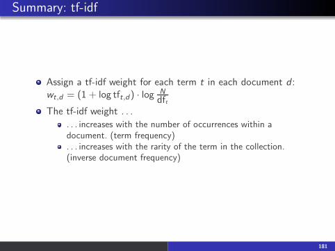
Summary: tf-idf
Assign a tf-idf weight for each term t in each document d :wt,d = (1 + log tft,d) · log N
dftThe tf-idf weight . . .
. . . increases with the number of occurrences within adocument. (term frequency). . . increases with the rarity of the term in the collection.(inverse document frequency)
181

Overview
1 Recap
2 Why ranked retrieval?
3 Term frequency
4 Zipf’s Law and tf-idf weighting
5 The vector space model

Binary incidence matrix
Anthony Julius The Hamlet Othello Macbeth . . .and Caesar Tempest
CleopatraAnthony 1 1 0 0 0 1Brutus 1 1 0 1 0 0Caesar 1 1 0 1 1 1Calpurnia 0 1 0 0 0 0Cleopatra 1 0 0 0 0 0mercy 1 0 1 1 1 1worser 1 0 1 1 1 0. . .
Each document is represented as a binary vector ∈ {0, 1}|V |.
182

Count matrix
Anthony Julius The Hamlet Othello Macbeth . . .and Caesar Tempest
CleopatraAnthony 157 73 0 0 0 1Brutus 4 157 0 2 0 0Caesar 232 227 0 2 1 0Calpurnia 0 10 0 0 0 0Cleopatra 57 0 0 0 0 0mercy 2 0 3 8 5 8worser 2 0 1 1 1 5. . .
Each document is now represented as a count vector ∈ N|V |.
183
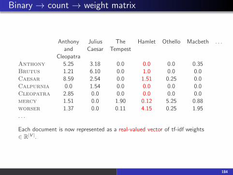
Binary → count → weight matrix
Anthony Julius The Hamlet Othello Macbeth . . .and Caesar Tempest
CleopatraAnthony 5.25 3.18 0.0 0.0 0.0 0.35Brutus 1.21 6.10 0.0 1.0 0.0 0.0Caesar 8.59 2.54 0.0 1.51 0.25 0.0Calpurnia 0.0 1.54 0.0 0.0 0.0 0.0Cleopatra 2.85 0.0 0.0 0.0 0.0 0.0mercy 1.51 0.0 1.90 0.12 5.25 0.88worser 1.37 0.0 0.11 4.15 0.25 1.95. . .
Each document is now represented as a real-valued vector of tf-idf weights∈ R
|V |.
184
Documents as vectors
Each document is now represented as a real-valued vector oftf-idf weights ∈ R
|V |.
So we have a |V |-dimensional real-valued vector space.
Terms are axes of the space.
Documents are points or vectors in this space.
Very high-dimensional: tens of millions of dimensions whenyou apply this to web search engines
Each vector is very sparse - most entries are zero.
185
Queries as vectors
Key idea 1: do the same for queries: represent them as vectorsin the high-dimensional space
Key idea 2: Rank documents according to their proximity tothe query
proximity ≈ negative distance
This allows us to rank relevant documents higher thannonrelevant documents
186

How do we formalize vector space similarity?
First cut: (negative) distance between two points
( = distance between the end points of the two vectors)
Euclidean distance?
Euclidean distance is a bad idea . . .
. . . because Euclidean distance is large for vectors of differentlengths.
187

Why distance is a bad idea
0 10
1
rich
poor
q: [rich poor]
d1:Ranks of starving poets swelld2:Rich poor gap grows
d3:Record baseball salaries in 2010
The Euclidean distance of ~q and ~d2 is large although thedistribution of terms in the query q and the distribution of terms inthe document d2 are very similar.
188
Use angle instead of distance
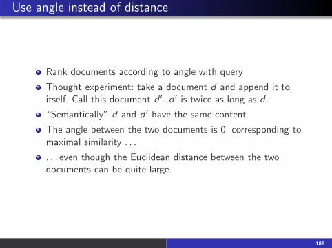
Rank documents according to angle with query
Thought experiment: take a document d and append it toitself. Call this document d ′. d ′ is twice as long as d .
“Semantically” d and d ′ have the same content.
The angle between the two documents is 0, corresponding tomaximal similarity . . .
. . . even though the Euclidean distance between the twodocuments can be quite large.
189

From angles to cosines
The following two notions are equivalent.
Rank documents according to the angle between query anddocument in decreasing orderRank documents according to cosine(query,document) inincreasing order
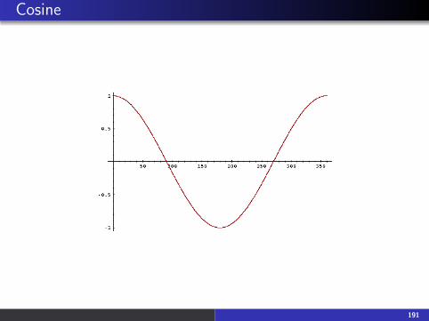
Cosine is a monotonically decreasing function of the angle forthe interval [0◦, 180◦]
190
Cosine
191

Length normalization
How do we compute the cosine?
A vector can be (length-) normalized by dividing each of itscomponents by its length – here we use the L2 norm:
||x ||2 =√
∑
i x2i
This maps vectors onto the unit sphere . . .
. . . since after normalization: ||x ||2 =√
∑
i x2i = 1.0
As a result, longer documents and shorter documents haveweights of the same order of magnitude.
Effect on the two documents d and d ′ (d appended to itself)from earlier slide: they have identical vectors afterlength-normalization.
192
Cosine similarity between query and document
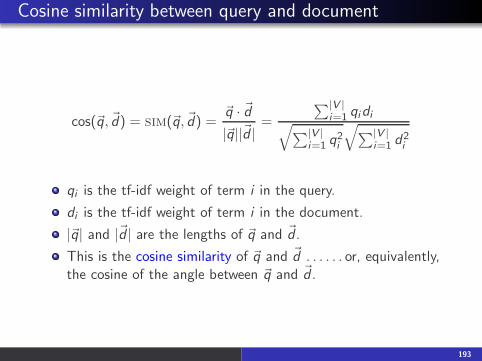
cos(~q, ~d) = sim(~q, ~d) =~q · ~d|~q||~d |
=
∑|V |i=1 qidi
√
∑|V |i=1 q
2i
√
∑|V |i=1 d
2i
qi is the tf-idf weight of term i in the query.
di is the tf-idf weight of term i in the document.
|~q| and |~d | are the lengths of ~q and ~d .
This is the cosine similarity of ~q and ~d . . . . . . or, equivalently,the cosine of the angle between ~q and ~d .
193

Cosine for normalized vectors
For normalized vectors, the cosine is equivalent to the dotproduct or scalar product.
cos(~q, ~d) = ~q · ~d =∑
i qi · di(if ~q and ~d are length-normalized).
194

Cosine similarity illustrated
0 10
1
rich
poor
~v(q)
~v(d1)
~v(d2)
~v(d3)
θ
195

Cosine: Example
How similar are thefollowing novels?
SaS: Sense andSensibility
PaP: Pride andPrejudice
WH: Wuthering Heights
Term frequencies (raw counts)
term SaS PaP WH
affection 115 58 20jealous 10 7 11gossip 2 0 6wuthering 0 0 38
196
Cosine: Example
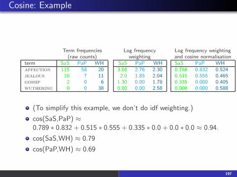
a Term frequenciesa (raw counts)
term SaS PaP WHaffection 115 58 20jealous 10 7 11gossip 2 0 6wuthering 0 0 38
Log frequencyweighting
SaS PaP WH3.06 2.76 2.302.0 1.85 2.04
1.30 0.00 1.780.00 0.00 2.58
Log frequency weightingand cosine normalisationSaS PaP WH0.789 0.832 0.5240.515 0.555 0.4650.335 0.000 0.4050.000 0.000 0.588
(To simplify this example, we don’t do idf weighting.)
cos(SaS,PaP) ≈0.789 ∗ 0.832 + 0.515 ∗ 0.555 + 0.335 ∗ 0.0 + 0.0 ∗ 0.0 ≈ 0.94.
cos(SaS,WH) ≈ 0.79
cos(PaP,WH) ≈ 0.69
197

Computing the cosine score
198

Components of tf-idf weighting
Term frequency Document frequency Normalization
n (natural) tft,d n (no) 1 n (none)1
l (logarithm) 1 + log(tft,d ) t (idf) log N
dftc (cosine)
1√w21+w2
2+...+w2M
a (augmented) 0.5 +0.5×tft,dmaxt(tft,d )
p (prob idf) max{0, log N−dftdft
} u (pivotedunique)
1/u
b (boolean)
{
1 if tft,d > 00 otherwise
b (byte size) 1/CharLengthα,α < 1
L (log ave)1+log(tft,d )
1+log(avet∈d(tft,d ))
Best known combination of weighting options
Default: no weighting
199

tf-idf example
We often use different weightings for queries and documents.
Notation: ddd.qqq
Example: lnc.ltn
Document:l ogarithmic tfn o df weightingc osine normalization
Query:l ogarithmic tft – means idfn o normalization
200

tf-idf example: lnc.ltn
Query: “best car insurance”. Document: “car insurance auto insurance”.
word query document producttf-raw tf-wght df idf weight tf-raw tf-wght weight n’lized
auto 0 0 5000 2.3 0 1 1 1 0.52 0best 1 1 50000 1.3 1.3 0 0 0 0 0car 1 1 10000 2.0 2.0 1 1 1 0.52 1.04insurance 1 1 1000 3.0 3.0 2 1.3 1.3 0.68 2.04
Key to columns: tf-raw: raw (unweighted) term frequency, tf-wght: logarithmically weightedterm frequency, df: document frequency, idf: inverse document frequency, weight: the finalweight of the term in the query or document, n’lized: document weights after cosinenormalization, product: the product of final query weight and final document weight√12 + 02 + 12 + 1.32 ≈ 1.92
1/1.92 ≈ 0.521.3/1.92 ≈ 0.68
Final similarity score between query and document:∑
i wqi · wdi = 0 + 0 + 1.04 + 2.04 = 3.08
201

Summary: Ranked retrieval in the vector space model
Represent the query as a weighted tf-idf vector
Represent each document as a weighted tf-idf vector
Compute the cosine similarity between the query vector andeach document vector
Rank documents with respect to the query
Return the top K (e.g., K = 10) to the user
202

Reading
MRS, chapter 5.1.2 (Zipf’s Law)
MRS, chapter 6 (Term Weighting)
203