MechanicsPhysics 151

Lecture 4Hamilton’s Principle

(Chapter 2)

Administravia

! Problem Set #1 due! Solutions will be posted on the web after this lecture

! Problem Set #2 is here! Due next Thursday

! Next lecture (Tuesday) will be given by Srinivas and Abdol-Reza! I will be attending a workshop at Stanford

What We Did Last Time

! Derived Lagrange’s Eqn from Newton’s Eqn! Using D’Alembert’s Principle = differential approach

! Lagrange’s Equations work if! Constraints are holonomic " Generalized coordinates! Forces of constraints do no work " No frictions! Other forces are monogenic " Generalized potential

jj j

U d UQq dt q

∂ ∂= − + ∂ ∂ !

Today’s Goals

! Discuss Hamilton’s Principle! Derive Lagrange’s Eqn from Hamilton’s Principle! Calculus of variation! Looks unfamiliar, but not so difficult

! Discuss conservation laws again! Using Lagrangian formalism! Linear, angular momenta! Connection between symmetry, invariance of the

Lagrangian, and conservation of generalized momentum

Configuration Space

! Generalized coordinates q1,...,qn fully describe the system’s configuration at any moment

! Imagine an n-dimensional space! Each point in this space (q1,...,qn)

corresponds to one configuration of the system! Time evolution of the system " A curve in the

configuration space

configurationspace

real space configuration space

Action Integral

! A system is moving as! Lagrangian is

! Action I depends on the entire path from t1 to t2! Choice of coordinates qj does not matter

! Action is invariant under coordinate transformation

( ) 1...j jq q t j n= =

( , , ) ( ( ), ( ), ) ( )L q q t L q t q t t L t= =! !

integrate2

1

t

tI Ldt= ∫ Action, or action integral

Hamilton’s Principle

! This is equivalent to Lagrange’s Equations! We will prove this

! Three equivalent formulations! Newton’s Eqn depends explicitly on x-y-z coordinates! Lagrange’s Eqn is same for any generalized coordinates! Hamilton’s Principle refers to no coordinates

! Everything is in the action integral

The action integral of a physical system is stationaryfor the actual path

We will also define “stationary”

Hamilton’s Principle is more fundamental probably...

Stationary

! Consider two paths that are close to each other! Difference is infinitesimal

! Stationary means that thedifference of the action integrals iszero to the 1st order of δq(t)! Similar to “first derivative = 0”

! Almost same as saying “minimum”! It could as well be maximum

configuration space

1t

2t

( )q t

( ) ( )q t q tδ+2 2

1 1

( , , ) ( , , ) 0t t

t tI L q q q q t dt L q q t dtδ δ δ= + + − =∫ ∫! ! !

1 2( ) ( ) 0q t q tδ δ= =

Infinitesimal Path Difference

! What’s δq(t)?! It’s arbitrary … sort of! It has to be zero at t1 and t2! It’s well-behaving

! Have to shrink it to zero! Trick: write it as

! α is a parameter, which we’ll make " 0! η(t) is an arbitrary well-behaving function

configuration space

1t

2t

( )q t

( ) ( )q t q tδ+Continuous, non-singular,continuous 1st and 2nd derivatives

( ) ( )q t tδ αη=

1 2( ) ( ) 0t tη η= =

Don’t worry too much

Hamilton " Lagrange

! Consider 1 generalized coordinate q! Add δq(t) to q(t), then make δq(t) " 0! Do this by

! α is a parameter " 0! η(t) is an arbitrary well-behaving

function

! Let’s define

( ) ( )q t tδ αη=

Continuous, non-singular,continuous η' and η''

2

1

( ) ( ( , ), ( , ), )t

tI L q t q t t dtα α α≡ ∫ !

( , ) ( ) ( )q t q t tα αη= +

1 2( ) ( ) 0t tη η= =

configuration space

1t

2t

( )q t

( ) ( )q t q tδ+

NB: this also depends on η(t)

Calculus of Variations! Let’s define

! If the action is stationary

2

1( ) ( ( , ), ( , ), )

t

tI L q t q t t dtα α α= ∫ !

0

( ) 0dId α

αα =

=

2

1

( ) t

t

dI L dq L dq dtd q d q d

αα α α

∂ ∂= + ∂ ∂ ∫

!!

Some work!

2

1

t

t

L d L dq dtq dt q dα

∂ ∂= − ∂ ∂ ∫ !

( )tη=

( , ) ( ) ( )q t q t tα αη= +

Arbitrary function

for any η(t)

NB: this also depends on η(t)

Lagrange’s Equation

! Fundamental lemma

! We got

2

1

( ) ( ) 0 for any ( )x

xM x x dx xη η=∫ 1 2( ) 0 for M x x x x= < <

2

1( ) 0

t

t

L d L t dtq dt q

η ∂ ∂− = ∂ ∂ ∫ !

0L d Lq dt q

∂ ∂− =∂ ∂ !

Done!

Notation of Variation

! For shorthand, we use δ for infinitesimal variation! I.e. α-derivative at α = 0

! Hamilton’s Principle can be written as2

10

t

t

L d LI qdtq dt q

δ δ ∂ ∂= − = ∂ ∂ ∫ !

0

( )dqq d t dd α

δ α η αα =

≡ =

( )2

10

( ( , ), ( , ), )t

t

dI dI d L q t q t t dt dd dα

δ α α α αα α=

≡ = ∫ !

Going Multi-Coordinates

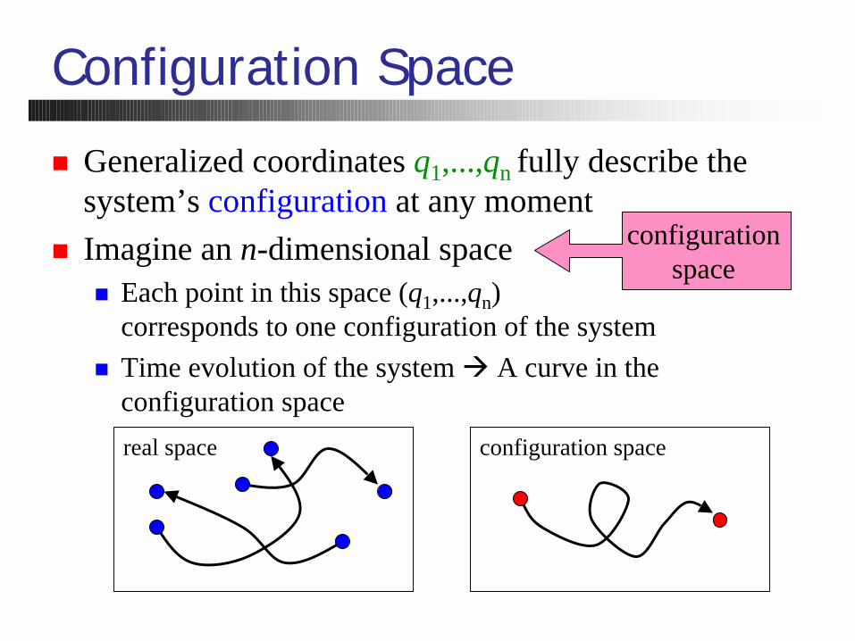
! Trivial to expand q " (q1, q2, …, qn)! See Goldstein Section 2.3

! Assumption: δq1, δq2, … are arbitrary and independent! Not true for x-y-z coordinates if there are constraints! True for generalized coordinates if the system is

holonomic

2

10

t

iti i i

L d LI q dtq dt q

δ δ ∂ ∂= − = ∂ ∂

∑∫ !

= 0 for each i

Hamilton’s Principle

! Action I describes the entire motion of the system! It is sufficient to derive the equations of motion

! Action I does not depend on the choice of the coordinates! Lagrange formalism is coordinate invariant

! Adding dF/dt to L would add F(t2) – F(t1) to I! It wouldn’t affect δI Variations are 0 at t1 and t2

! Arbitrarity of L is obvious

2

1

( , , ) 0t

tI L q q t dtδ δ= =∫ !

( , )dF q tL Ldt

′ = +

Calculus of Variation

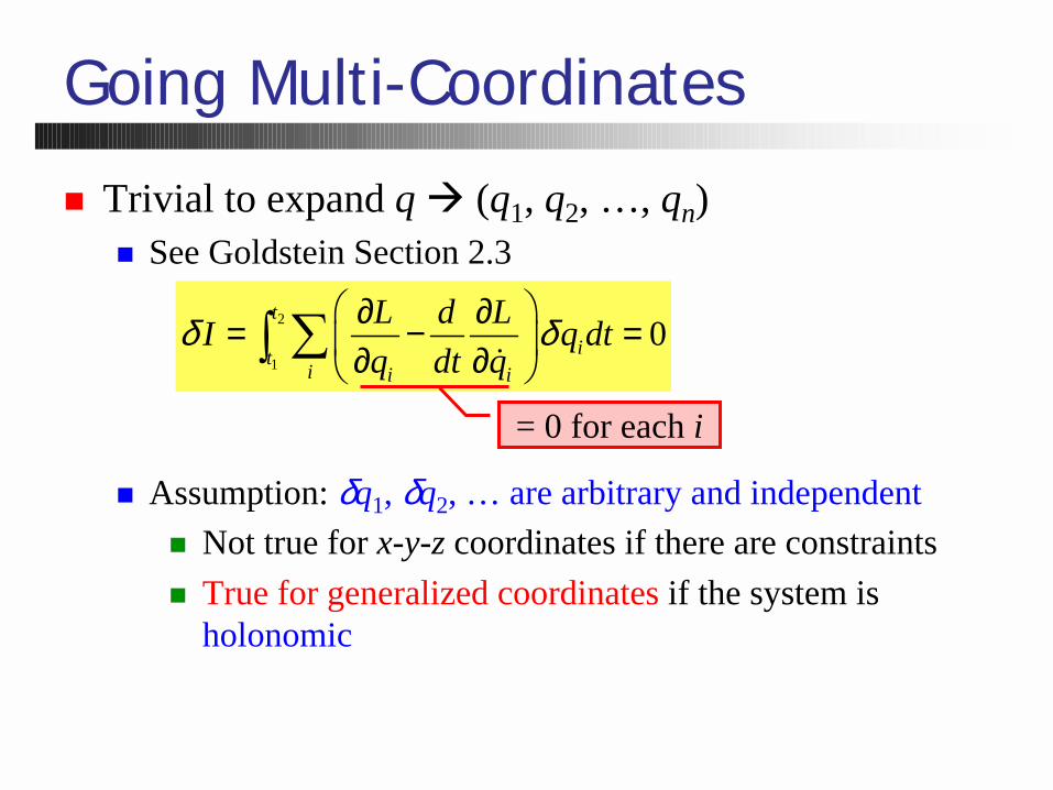
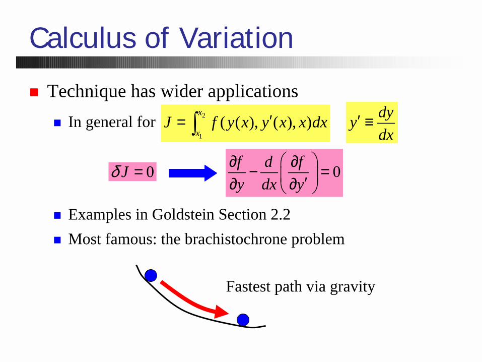
! Technique has wider applications! In general for

! Examples in Goldstein Section 2.2! Most famous: the brachistochrone problem

0Jδ =

dyydx

′ ≡2

1

( ( ), ( ), )x

xJ f y x y x x dx′= ∫

0f d fy dx y

∂ ∂− = ′∂ ∂

Fastest path via gravity

Conservation Laws

! We’ve seen (in Lectures 1&2) conservation of linear, angular momenta and energy in Newtonian mechanics! How do they work with Lagrange’s equations?! Should better be the same…

! We’ll find a few differences and assumptions! They are, in fact, limitations we ignored so far

Momentum Conservation

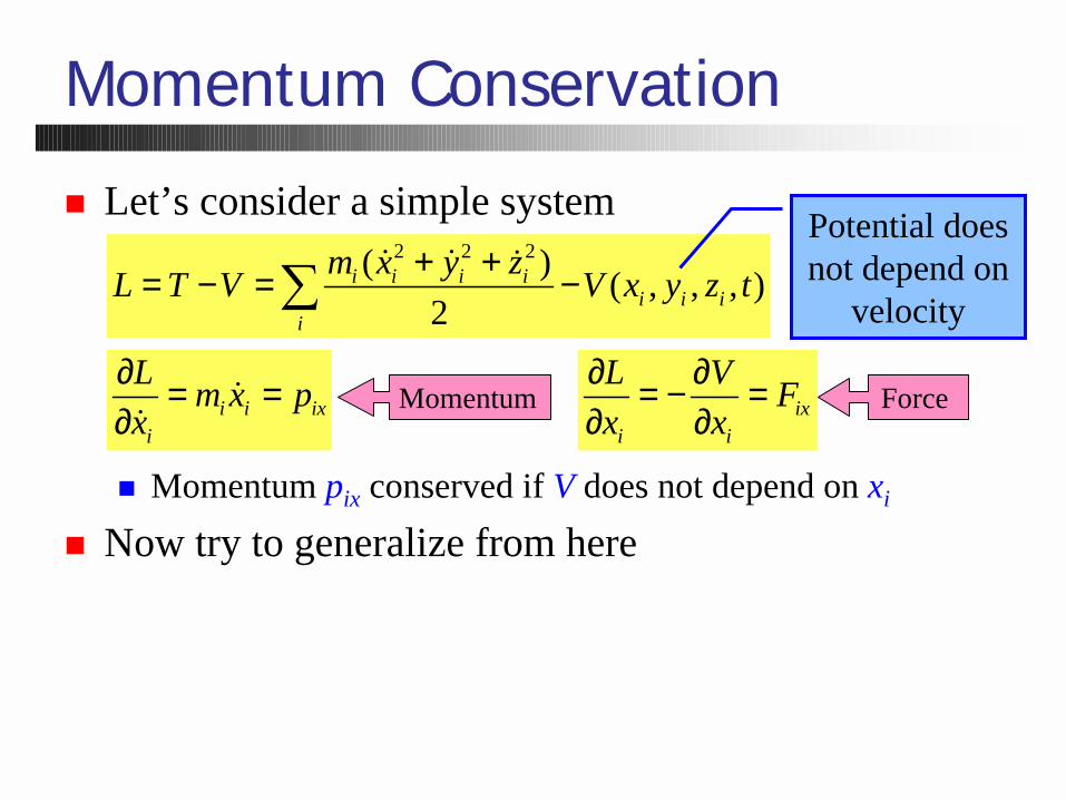
! Let’s consider a simple system

! Momentum pix conserved if V does not depend on xi

! Now try to generalize from here

2 2 2( ) ( , , , )2

i i i ii i i

i

m x y zL T V V x y z t+ += − = −∑ ! ! !Potential does not depend on

velocity

i i ixi

L m x px

∂ = =∂

!! ix

i i

L V Fx x

∂ ∂= − =∂ ∂

Momentum Force

Generalized Momentum

! Let’s call the generalized momentum

! Also known as canonical or conjugate momentum! Equals to usual momentum for simple x-y-z coordinates

! Lagrange’s equation becomes

! pj is conserved if L does not depend explicitly on qj

! Such qj is called cyclic (or ignorable)

jj

Lpq

∂≡∂ !

0j

j

dp Ldt q

∂− =∂

Generalized momentum associated with a cyclic coordinate is conserved

Linear momentumconservation is a

special case

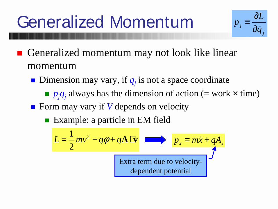
Generalized Momentum

! Generalized momentum may not look like linear momentum! Dimension may vary, if qj is not a space coordinate

! pjqj always has the dimension of action (= work × time)! Form may vary if V depends on velocity

! Example: a particle in EM field

jj

Lpq

∂≡∂ !

212

L mv q qφ= − + ⋅A v x xp mx qA= +!

Extra term due to velocity-dependent potential

Symmetry

! Linear momentum p = (px, py, pz) is conjugate of(x, y, z) coordinates! Conserved if Lagrangian does not depend explicitly on

position! I.e. if Lagrangian is invariant under space translation

! Such a system is called symmetric under space translation

! Symmetry of a system = Invariance of Lagrangian" Conservation of conjugate momentum! Let’s study an example of angular momentum

( , , ) ( , , )x y z x x y y z z→ + ∆ + ∆ + ∆

Angular Momentum

! Consider a multi-particle system! Suppose q1 turns the whole system around

! Example: φ in! Assume V does not depend on

! Conjugate momentum is

1( ,..., , )i i nq q t=r r

( , , ) ( cos , sin , )i i i i i i ix y z r r zφ φ= =r

iz

ir

dφ

( )i φr

( )i dφ φ+r

φ!

L Tpφ φ φ∂ ∂≡ =∂ ∂! !

ii

= ⋅ = ⋅∑n L n Lbit ofwork

Axis of rotation Total angular momentum

n

Bit of Work

! dri is perpendicular to both n and ri

! Size of dri is ri sinθ dφ

2i

i ii

mT = ⋅∑ r r! !

2

ni i i

i kk k

qq t

φφ =

∂ ∂ ∂= + +∂ ∂ ∂∑r r rr !! ! i i

φ φ∂ ∂=∂ ∂r r!!

2( , ,..., , )i i nq q tφ=r r

i ii i i i

i i

T m mφ φ φ

∂ ∂∂ = ⋅ = ⋅∂ ∂ ∂∑ ∑r rr r

!! !! !

n

dφ

iridr

θ

iiφ

∂ = ×∂r n r

( )

( )

i i ii

i i i ii i

m

m

= ⋅ ×

= ⋅ × = ⋅

∑

∑ ∑

r n r

n r r n L

!

!

Angular Momentum

! Angular momentum is conserved if the system is symmetric under rotation! How does this relate to the total torque N?

! T cannot depend on φ Rotating doesn’t change

LQφ φ∂≡∂

Generalizedforce

This must be zero if φ is cyclic

2iv

( )ii i i i i

i i i

L Vφ φ φ

∂∂ ∂= − = = ⋅ × = ⋅ ×∂ ∂ ∂∑ ∑ ∑rF F n r n r F

TorqueTotal torque is zero along the axis of symmetry

Conservation Laws

! Following statements are equivalent:! System is symmetric wrt a generalized coordinate! The coordinate is cyclic (does not appear in Lagrangian)! The conjugate generalized momentum is conserved! The associated generalized force is zero

TorqueForceForceAngularLinearMomentumAngle around an axisDistance along an axisCoordinateRotationSpatial translationSymmetry

Summary

! Derived Lagrange’s Eqn from Hamilton’s Principle! Calculus of variation

! Discussed conservation laws! Generalized (conjugate) momentum! Symmetry of the system" Invariance of the Lagrangian" Conservation of momentum

! We are almost done with the basic concepts! Finish up next Tuesday with energy conservation! Some applications are in order " Central force problem

jj

Lpq

∂≡∂ !