Lecture 33normal distribution statistics

8/13/2019 Lecture 33normal distribution statistics

http://slidepdf.com/reader/full/lecture-33normal-distribution-statistics 1/6

Numerical Integration of a Normal Distribution

A Normal Distribution:

∫=≤≤ b

a

dx).x(f ) bXa(P

⎥⎦⎤⎢

⎣⎡

σμ−−

σπ=σμ 2

2

.2)x(exp.

.21),:x(f

0

A Standard Normal Distribution:

∞∞− x

=≤≤ b

dz.zf bZaPa

⎥⎦

⎤⎢⎣

⎡−

π=

.2

zexp.

.2

1)1,0:z(f

2 = 0; σ = 1

+∞≤≤∞− z0

This function has been integrated numerically,and the results have been tabulated.



0.00 0.01 0.02 0.03 0.04 0.05 0.06 0.07 0.08 0.09

0.0 0.0000 0.0040 0.0080 0.0120 0.0160 0.0199 0.0239 0.0279 0.0319 0.0359

0.1 0.0398 0.0438 0.0478 0.0517 0.0557 0.0596 0.0636 0.0675 0.0714 0.0753

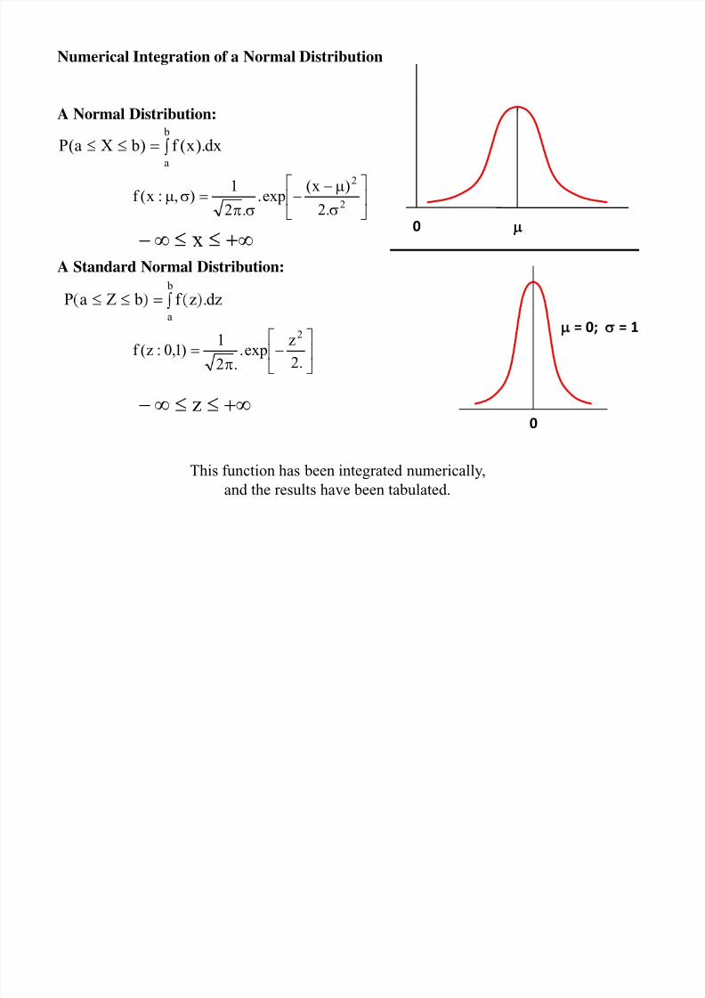
Standard Normal Table

. . . . . . . . . . .

0.3 0.1179 0.1217 0.1255 0.1293 0.1331 0.1368 0.1406 0.1443 0.1480 0.1517

0.4 0.1554 0.1591 0.1628 0.1664 0.1700 0.1736 0.1772 0.1808 0.1844 0.1879

0.5 0.1915 0.1950 0.1985 0.2019 0.2054 0.2088 0.2123 0.2157 0.2190 0.2224

0.6 0.2257 0.2291 0.2324 0.2357 0.2389 0.2422 0.2454 0.2486 0.2517 0.2549

0.7 0.2580 0.2611 0.2642 0.2673 0.2704 0.2734 0.2764 0.2794 0.2823 0.2852

0.8 0.2881 0.2910 0.2939 0.2967 0.2995 0.3023 0.3051 0.3078 0.3106 0.3133

0.9 0.3159 0.3186 0.3212 0.3238 0.3264 0.3289 0.3315 0.3340 0.3365 0.33891.0 0.3413 0.3438 0.3461 0.3485 0.3508 0.3531 0.3554 0.3577 0.3599 0.3621

1.1 0.3643 0.3665 0.3686 0.3708 0.3729 0.3749 0.3770 0.3790 0.3810 0.3830

1.2 0.3849 0.3869 0.3888 0.3907 0.3925 0.3944 0.3962 0.3980 0.3997 0.4015

1.3 0.4032 0.4049 0.4066 0.4082 0.4099 0.4115 0.4131 0.4147 0.4162 0.4177

1.4 0.4192 0.4207 0.4222 0.4236 0.4251 0.4265 0.4279 0.4292 0.4306 0.4319

1.5 0.4332 0.4345 0.4357 0.4370 0.4382 0.4394 0.4406 0.4418 0.4429 0.4441

1.6 0.4452 0.4463 0.4474 0.4484 0.4495 0.4505 0.4515 0.4525 0.4535 0.45451.7 0.4554 0.4564 0.4573 0.4582 0.4591 0.4599 0.4608 0.4616 0.4625 0.4633

X0

. . . . . . . . . . .

1.9 0.4713 0.4719 0.4726 0.4732 0.4738 0.4744 0.4750 0.4756 0.4761 0.4767

2.0 0.4772 0.4778 0.4783 0.4788 0.4793 0.4798 0.4803 0.4808 0.4812 0.4817

2.1 0.4821 0.4826 0.4830 0.4834 0.4838 0.4842 0.4846 0.4850 0.4854 0.4857

2.2 0.4861 0.4864 0.4868 0.4871 0.4875 0.4878 0.4881 0.4884 0.4887 0.4890

. . . . . . . . . . .

2.4 0.4918 0.4920 0.4922 0.4925 0.4927 0.4929 0.4931 0.4932 0.4934 0.4936

2.5 0.4938 0.4940 0.4941 0.4943 0.4945 0.4946 0.4948 0.4949 0.4951 0.4952

2.6 0.4953 0.4955 0.4956 0.4957 0.4959 0.4960 0.4961 0.4962 0.4963 0.4964

2.7 0.4965 0.4966 0.4967 0.4968 0.4969 0.4970 0.4971 0.4972 0.4973 0.4974

2.8 0.4974 0.4975 0.4976 0.4977 0.4977 0.4978 0.4979 0.4979 0.4980 0.4981

2.9 0.4981 0.4982 0.4982 0.4983 0.4984 0.4984 0.4985 0.4985 0.4986 0.4986

3.0 0.4987 0.4987 0.4987 0.4988 0.4988 0.4989 0.4989 0.4989 0.4990 0.4990

Because the curve is symmetrical, the same table can be used for values going

either direction, so a negative 0.45 also has an area of 0.1736



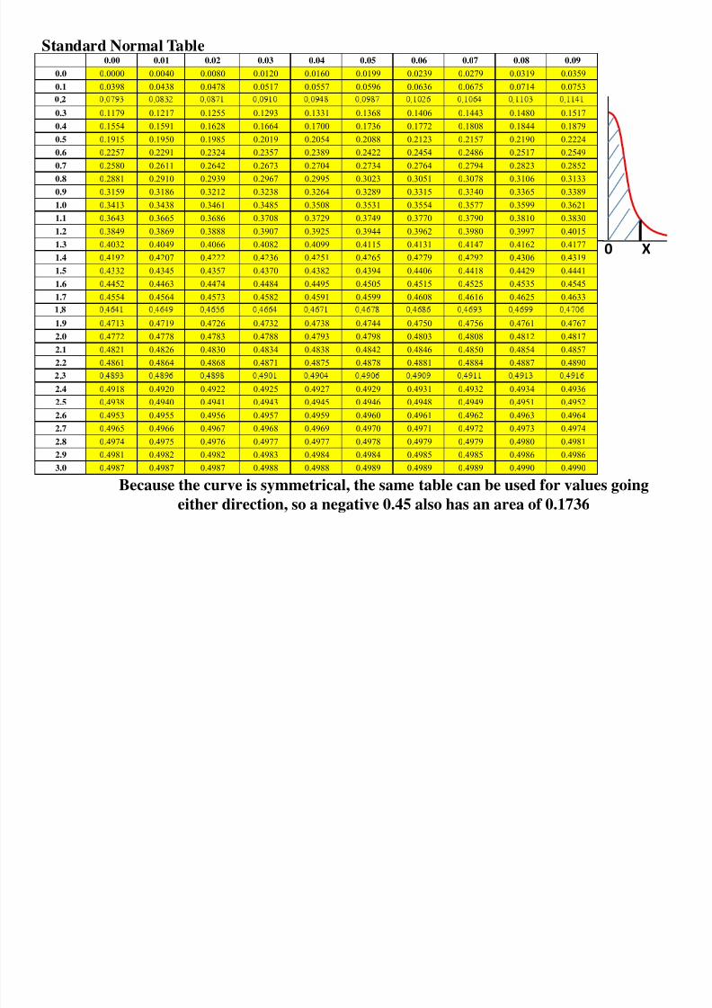
)25.1Z(P >Calculate:

P(Z 1.25)> Area of the standard normal curve to the right of Z = 1.25

1.000 - 0.500 - 0.3944 = 0.10561 P(Z 0.0) P(0.0 Z 1.25)− ≤ − ≤ ≤ =

= 0 σ = 1

Calculate: P( 0.38 Z 1.25)− ≤ ≤

= 0;

σ = 1

0 X = 1.25

0

X = 1.25X = ‐0.38

)25.1Z38.0(P ≤≤− = 0.3944 + 0.1480 = 0.5424



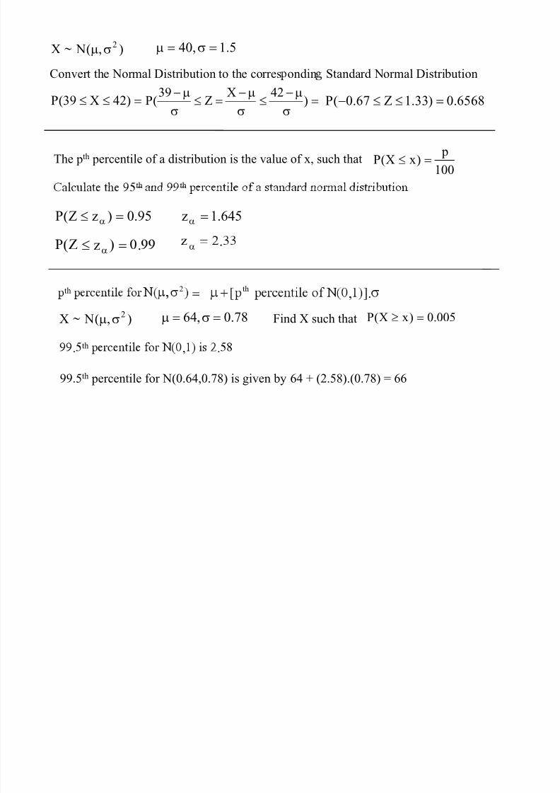
),( N~X 2σμ 5.1,40 =σ=μ

Convert the Normal Distribution to the corres ondin Standard Normal Distribution

P(39 X 42)≤ ≤ = 39 X 42P( Z )

− μ − μ − μ≤ = ≤ =

σ σ σ P( 0.67 Z 1.33) 0.6568− ≤ ≤ =

The pth percentile of a distribution is the value of x, such that100 p)xX(P =≤

th th

95.0)zZ(P =≤ α 645.1z =α

.z =≤ α .α

2 =th th , .

),( N~X 2σμ 64, 0.78μ = σ = Find X such that 005.0)xX(P =≥

th. , .

99.5th percentile for N(0.64,0.78) is given by 64 + (2.58).(0.78) = 66



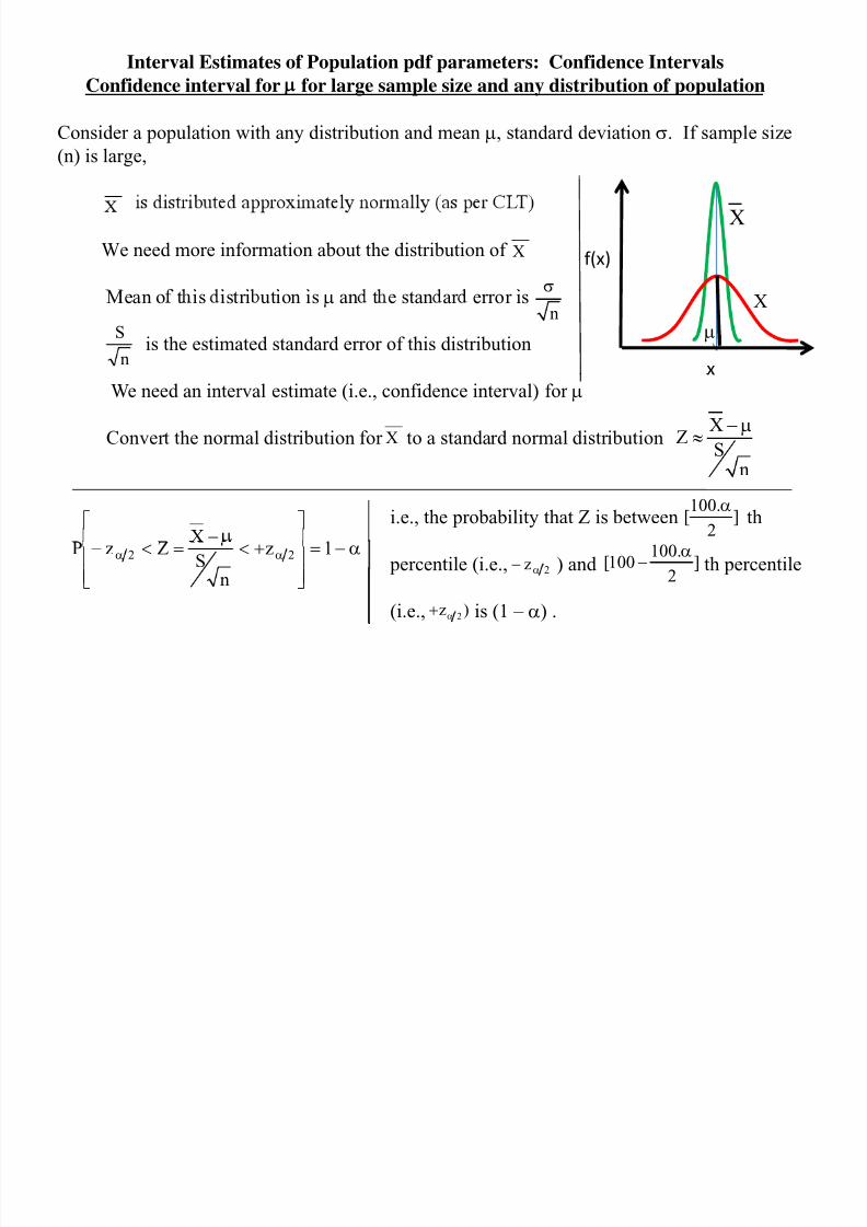
Interval Estimates of Population pdf parameters: Confidence Intervals

Confidence interval for for large sample size and any distribution of population

Consider a population with any distribution and mean μ, standard deviation σ. If sample size

(n) is large,

We need more information about the distribution of

X

f(x)X

Mean o t is istri ution is μ an t e stan ar error is

is the estimated standard error of this distributionn

S

x

μ

Xn

We need an interval estimate (i.e., confidence interval) for μ

Convert the normal distribution for to a standard normal distribution X

ZS

− μ≈X

n

⎤⎡−X

i.e., the probability that Z is between th100.

[ ]2

α

α−=

⎥

⎥

⎦⎢

⎢

⎣

+<=<− αα 1z

n

SZzP 22

percentile (i.e., ) and th percentile

(i.e., is (1 – α) .

2zα− 100.

[100 ]

2

α−

2z )α+



α−=⎥⎦

⎤⎢⎣

⎡+<μ<− αα 1)]

n

S.z(X[)]

n

S.z(X[P 22

Please note that the value of the confidence interval depends on and S, which are

random variables. Thus the confidence interval is itself random. This is what the

X

α−=⎥⎦

⎤⎢⎣

⎡ +<μ<− αα 1)]n

S.z(X[)]

n

S.z(X[P 22

express on,

actually mean,

If a large number of intervals were constructed by repeated ⎥⎦

⎤

⎢⎣

⎡

+− αα )]n

S

.z(X[)],n

S

.z(X[ 22

sampling from a population, then in the long run, the percentage of intervals containing the

population mean (which remains unknown) is (1 – α).100.

Example:The mean of an experimental measurement on 56 samples is 8.17 with standard error of

1.42. What is the 95% confidence interval on population mean.

37.017.8

56

...17.8 ±=±

Documents

Lecture 33normal distribution statistics