Lecture 3: Decision TreeInstructor: Prof. Shuai Huang

Industrial and Systems Engineering

University of Washington

Decision tree

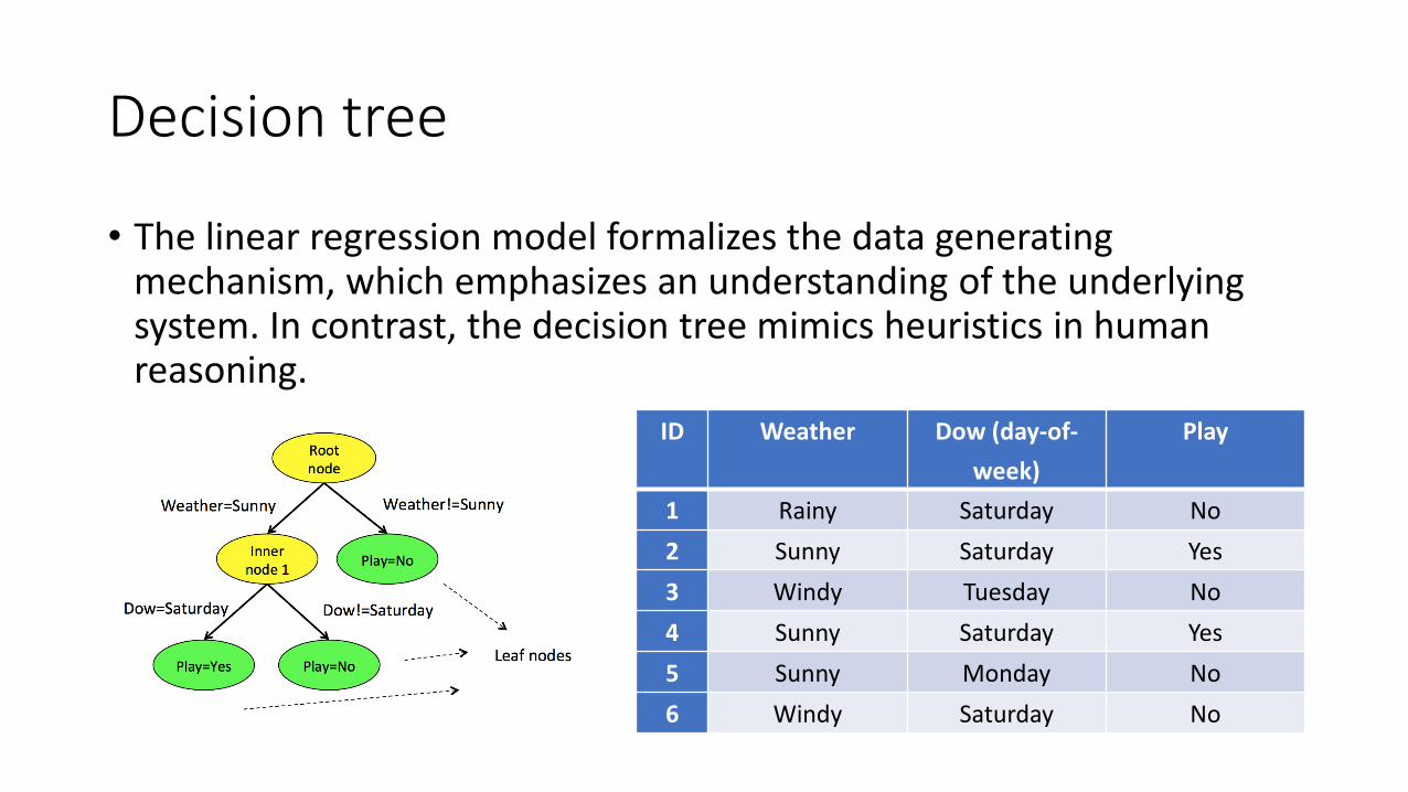
• The linear regression model formalizes the data generating mechanism, which emphasizes an understanding of the underlying system. In contrast, the decision tree mimics heuristics in human reasoning.

ID Weather Dow (day-of-

week)

Play

1 Rainy Saturday No

2 Sunny Saturday Yes

3 Windy Tuesday No

4 Sunny Saturday Yes

5 Sunny Monday No

6 Windy Saturday No

A recursive splitting procedure

• A key element of a decision tree is the splitting rules that can lead us through the inner nodes to the final decision node to reach a decision

• E.g., for the exemplary dataset, possible splitting rules are {Weather = Rainy, Weather = Sunny, Dow = Saturday, Dow = Monday, Dow = Tuesday}

Entropy as a measure of Impurity

• For classification problem (the outcome variable is categorical), the impurity of data points in a given node can be measured by entropy:

𝑒 = σ𝑖=1,..,𝐾−𝑃𝑖𝑙𝑜𝑔2𝑃𝑖.

• 𝐾 represents the number of classes and 𝑃𝑖 is the proportion of data points in the node that belong to the class 𝑖. The entropy 𝑒 is defined as 0 when the data points in the node all belong to one single class.

Information gain (IG)

• A node having a large impurity is not ready to be a decision node yet.

• Thus, if we want to further split the node and create two more child nodes under it, we look for the best splitting rules that can minimize the impurity of the children nodes.

• This reduction of impurity can then be measured by information gain (IG), which is the difference of the entropy of the splitting node and the average entropy of the two children nodes weighted by their number of data points.

• The IG is defined as:

𝐼𝐺 = 𝑒𝑠 − σ𝑖=1,..,𝑛𝑤𝑖 ∗ 𝑒𝑖.

• Here, 𝑒𝑠 is the entropy at the splitting node, 𝑒𝑖 is the entropy at the child node 𝑖, and 𝑤𝑖 is the number of data points in the children node 𝑖 divided by the number of data points at the splitting node.

Apply IG on the exemplary dataset

Let’s look at the decision tree model in the left figure. The entropy of the root node is calculated as

−4

6𝑙𝑜𝑔2

4

6−

2

6𝑙𝑜𝑔2

2

6= 0.92.

The entropy of the left child node (“Weather = Sunny”) is

−2

3𝑙𝑜𝑔2

2

3−

1

3𝑙𝑜𝑔2

1

3= 0.92.

The entropy of the right child node (“Weather != Sunny”) is 0 since all the three data points (ID = 1,3,6) belong to the same class.

The information gain for the splitting rule “Weather = Sunny” is then

𝐼𝐺 = 0.92 −3

6∗ 0.92 −

3

6∗ 0 = 0.46.

Apply IG on the exemplary dataset – cont’d

For the decision tree in the right figure, the entropy of the left child node (“Dow = Saturday”) is

−2

4𝑙𝑜𝑔2

2

4−

2

4𝑙𝑜𝑔2

2

4= 1.

The entropy of the right child node (“Dow != Saturday”) is 0 since the two data points (ID = 3,5) belong to the same class.

Thus, the information gain for the splitting rule “Dow = Saturday” is then

𝐼𝐺 = 0.92 −3

6∗ 1 −

3

6∗ 0 = 0.42.

As the information gain of “Weather = Sunny” is higher, the splitting rule “Weather = Sunny” is preferred over its competitor “Dow = Saturday”.

Greedy nature of recursive splitting

• Based on the concept of impurity and IG, we could develop a greedy strategy that recursively split the data points until there is no further IG, e.g., when there is only one data point, or only one class in the node.

• Most tree-building methods use this approach, with difference in the definitions of the impurity and IG.

• However, this will inevitably lead to a very large decision tree with many inner nodes and unstable decision nodes (i.e., since the decisions assigned to these nodes are inferred empirically based on very few data points).

• Thus, such a decision tree can be sensitive to noisy data, leading to worse accuracy and interpretability.

Pruning of a tree

• To mitigate this problem, the pre-pruning or post-pruning methods can be used to control the complexity of a decision trees.

• Pre-pruning stops growing a tree when a pre-defined criterion is met. One can define the maximum depth of a tree, or minimum number of data points at each node.

• Since we can never anticipate the future growth of a tree, it is commonly perceived that pre-pruning can cause over-simplified and under-fitted tree models. In other words, it is too cautious.

• In contrast, post-pruning prunes a tree after it is fully-grown and has less risk of under-fit as a full-grown tree contains sufficient information captured from the data.

Post-pruning of a tree

• Post-pruning starts from the bottom of the tree. If removing the sub-tree of an inner node does not increase the error, then the sub-tree under the inner node can be pruned.

• Note that, the error here is not the error calculated based on the training data that is used to train the tree. This error calculated based on training data is called as empirical error.

• Rather, here, we should use the generalization error, that is, the error when applied to unseen data.

• Thus, in the famous decision tree algorithm, C4.5, the pessimistic error estimation approach is used.

Pessimistic error estimation

• Denote the empirical error rate on the training data as Ƹ𝑒, which is only an estimation of the generalization error 𝑒.

• Since each data point can be either correctly or wrongly classified, we can view the probability of being correctly classified as a binomial distribution with probability 𝑒.

• With this insight, the normal distribution approximation can be applied here to derive the confidence interval of the generalization error 𝑒 as:

Ƹ𝑒 − 𝑧 Τ𝛼 2Ƹ𝑒 1− Ƹ𝑒

𝑛≤ 𝑒 ≤ Ƹ𝑒 + 𝑧 Τ𝛼 2

Ƹ𝑒 1− Ƹ𝑒

𝑛.

• The upper bound of the interval, Ƹ𝑒 + 𝑧 Τ𝛼 2Ƹ𝑒 1− Ƹ𝑒

𝑛, is used as the estimate of 𝑒. As this is

an upper bound, it is named as pessimistic error estimation.

• Note that, the estimate of the error depends on three values, 𝛼, which is often set to be 0.25 so that 𝑧 Τ𝛼 2=1.15; Ƹ𝑒, which is the training error; and 𝑛, which is the number of data points at the node. Therefore, the estimated error is larger with a smaller 𝑛, accounting for the sample size as well.

An example

• Consider the inner node 1. We can see that, if we prune the subtree below inner node 1, we will label it with class C1, as 20 of the included data points are labeled as C1 while 19 are labeled as C2. And we can get that the total misclassified instances 𝑚 is 19. Thus, Ƹ𝑒 =

19

39= 0.4871.

• For the pessimistic error estimation, we can get that

Ƹ𝑒 + 𝑧 Τ𝛼 2Ƹ𝑒 1− Ƹ𝑒

𝑛= 0.4871 +

1.150.4871 1−0.4871

39= 0.579.

• Thus, we can get that 𝑚𝑝 = 0.579 × 39 = 22.59.

An example – cont’d

• Now, let’s see if the splitting of this inner node into its two child nodes improves the pessimistic error. It can be seen that, with this subtree of the two child nodes, the total misclassified instances 𝑚is 9+9=18. And by pessimistic error estimation, 𝑚𝑝 = 11.5 +11.56 = 23.06 for the subtree. Therefore, based on the pessimistic error, we should prune the subtree.

The parameter “cp” in the R package “rpart”

• Both pre-pruning and post-pruning are useful

• Pre-pruning tends to lead to oversimplified decision tree models. In this aspect, post-pruning seems to be more preferable, but not always.

• E.g, another popular strategy, as used in the “rpart” R package, the complexity parameter (cp) is used. Using the parameter, all splits need to improve the impurity score, e.g., information gain, by at least a factor of cp, that is, splits do not decrease the impurity score by cpwill not be pursued. This strategy also works well in many applications

R lab

• Download the markdown code from course website

• Conduct the experiments

• Interpret the results

• Repeat the analysis on other datasets