Lecture 2 MGMT 7730 - © 2011 Houman Younessi Derivatives Derivative of a constant Y X Y=3 Y1 X1X2

Lecture 2

MGMT 7730 - © 2011 Houman Younessi

Derivatives

Derivative of a constant

Y

X

Y=3Y1

012

0lim

0

XXdX

dYX

X1 X2

12

11limlim

00 XX

YY

X

Y

dX

dYXX

X

Y

dX

dYX

0lim

Lecture 2


Derivative of a line

Y

X

Y=5X

Y1=10

51

5

23

1015lim

0

XdX

dY

X1=2 X2=3

12

12limlim

00 XX

YY

X

Y

dX

dYXX

Y2=15

Lecture 2


Derivative of a polynomial function

1)3(

2)2(

1)1( ......)2()1( aXanXanXna

dX

dY nb

nb

nb

0)2(

2)1(

1 ...... aXaXaXaY nb

nb

nb

23XY

Examples:

XXdX

dY623 12

1323 XCXKXY 323 2 CXKXdX

dY

Lecture 2


Derivatives of sums and differencesIn general:

For )()()( xZxWxY )()()( xZxWxY

dX

dZ

dX

dW

dX

dY

or

dX

dZ

dX

dW

dX

dY

Lecture 2


Derivatives of products and quotientsIn general:

For )()()( xZxWxY )(/)()( xZxWxY

dX

dWZ

dX

dZW

dX

dY

or

2

)()(

ZdX

dZWdXdWZ

dX

dY

Examples:

)1(181818

61812

6)3()2(6

)3(6

3)(

6)(

)3(6)(

22

22

2

2

2

2

XX

XX

XXXdX

dYdX

dWX

dX

dZX

dX

dY

XxZ

XxW

XXxY

2

2

2

32

2

32

2

3

3

)43(

)4045(

)43(

4045

)43(

)4(5)15)(43(

4

15

43)(

5)(

43

5)(

X

XX

X

XX

X

XXX

dX

dY

dX

dZ

XdX

dW

XxZ

XxW

X

XxY

Lecture 2


Derivative of a derivative

0 Q1

Profit

Number of units of output

A

Q1

Profit

Number of units of output

A

0

)(2

2

dX

dY

dx

d

dX

Yd

6

46

143

2

2

2

dX

Yd

XdX

dY

XXY

8

78

374

2

2

2

dX

Yd

XdX

dY

XXY

Lecture 2


Partial DerivativeA derivate with respect to only one variable when the function is the

function of more than just that variable

A single variable function:

A multi-variable function:

181080

449

1243),(

22

223

XWXWW

Y

XWXX

Y

WXXWXwxY

49

143)(

2

3

XdX

dY

XXxY

Lecture 2


Optimization TheoryUnconstrained Optimization

Unconstrained optimization applies when we wish to find the maximum or minimum point of a curve. In other words we wish to find the value of the independent variable at which the dependent variable is maximized or minimized without any other external conditions restricting it.

Let us assume that there is an activity x which generates both value V(x) and cost C(x).

Net value would therefore be:

The necessary condition to find the optimal level is:

Or:

)()()( xCxVxNV

dx

xdC

dx

xdV

dx

xdNV )()(0

)(

dx

xdC

dx

xdV )()(

Lecture 2


Unconstrained Optimization: Multiple variables

In the case where there are more than one activity, say when the value function is a function of x and y, we take the derivative of the function with respect to each variable and set them all to zero.

0),(),(),(

0),(),(),(

),(),(),(

y

yxC

y

yxV

y

yxNVx

yxC

x

yxV

x

yxNV

yxCyxVyxNV

As such we have:

y

yxC

y

yxV

andx

yxC

x

yxV

),(),(

),(),(

Lecture 2


Example:

ABCO LLC has two product lines: gadgets and widgets.

ABCO produces G of gadgets and W of widgets annually

The profit made by ABCO is of course related to their quantity of widgets and gadgets sold. The following equation shows this relationship:

2075.1138010105),( 22 GWWGGWWGP

Find the derivative (partial derivative) of profit with respect to G.

75.113205

GWG

P

Lecture 2


Find the derivative (partial derivative) of profit with respect to W.

80205

WGW

P

Now, using this information find the quantities of G and W that ABCO must manufacture to maximize profit.

To answer this question, we remember that a point is either a maximum or minimum when the derivative for that point is zero. For P to be maximized both derivatives with respect to G and W must be zero.

75.2

0.5

080205

075.113205

W

G

WG

GW

Lecture 2


Constrained Optimization

Constrained optimization applies when we wish to find the maximum or minimum point of a curve but there are also other limiting factors. In other words we wish to find the value of the independent variable at which the dependent variable is maximized or minimized with other external conditions restricting it.

y

yxVand

x

yxV

),(),(Let us start – without loss of generality -with

the marginal value for a two variable case:

The constraint is that the total cost must equal a specified level of cost relating to the price and quantities of the two components x, and y:

CyPxPyxC yx ),(

Lecture 2


There are two equivalent ways of solving such problems:

1. Simple simultaneous equations:

In this approach we solve the set of equations:

0

0),(

0),(

CyPxP

y

yxVx

yxV

yx

2. Lagrangian method:

The Lagrangian method works on the basis of adding “meaningful zeros” to the original equation and then assess their impact.

Lecture 2


The first thing we do is to form the Lagrangian function.

To do so, we first rearrange our constraint formula or formulas so that they all evaluate to zero:

0

CyPxP

CyPxP

yx

yx

Then, we add “zero” to the original value function:

)(),( yPxPCyxVL yx

Now we take partial derivatives of the value function wrt x, y and λ, set these to zero and solve.

Lecture 2


Example:Cando Co wishes to minimize the cost of their production governed by:

2122

21 54 QQQQTC

The constraint is that the company can only make 30 units of product in total

03030 2121 QQorQQ

The Lagrangian becomes: )30(54 212122

21 QQQQQQL

As such we have:

030),,(

010),,(

08),,(

2121

212

21

211

21

QQQQL

QQQ

QQL

QQQ

QQL

Lecture 2


Solving

030

010

08

21

21

21

QQ

QQ

QQ

For Q1, Q2 and λ

We get: Q1=16.5

Q2=13.5

λ= 118.5

What does λ mean?

It means that if the constraint were to be relaxed so that more than 30 units could be produced, the cost of producing the 31st is $118.5

Lecture 2


Imagine that you are running a manufacturing plant. This plant has the capacity of making 30 units of either widgets or gadgets. Furthermore, the total cost of the manufacturing operation is:

GWWGC 22 54How many widgets and how many gadgets should you manufacture to minimize cost?

To minimize cost, we must find the minimum of the cost function above. We also must make sure that the total units manufactures equals 30.

As such:

WG

therefore

WG

30

30

Example 2:

Lecture 2


Substituting: WG 30 GWWGC 22 54

360027010

)30(5)30(42

22

WW

WWWWC

Into:

Taking the derivative and setting it to zero, we get:

5.165.1330

5.13

027020

G

W

or

WdW

dC

To make sure this is a minimum point:

020)( dW

dC

dW

d

Lecture 2


Market Demand and the Demand Function

Market Demand Schedule for laptops

Price per unit ($) Quantity demanded per year (‘000)

3000

2750

2500

2250

2000

800

975

1150

1325

1500

Lecture 2


2000

2500

3000

800 1000 1200 1400 1600

Demand CurvePrice

Quantity

Lecture 2


Influences on Demand

2000

2500

3000

800

1000

1200

1400

1600

Price

Quantity

Increase in customer preference for laptops

2000

2500

3000

800

1000

1200

1400

1600

Price

Quantity

Increase in customer per capita income

2000

2500

3000

800

1000

1200

1400

1600

Price

Quantity

Increase in advertising for laptops 2000

2500

3000

800

1000

1200

1400

1600

Price

Quantity

reduction in cost of software

Lecture 2


Demand Function

Q=f( price of X, Income of consumer, taste of consumer, advertising expenditure, price of associated goods,….)

Example:

Q= -700P+200I-500S+0.01Awhere

Demand for laptops in 2007 is estimated to be:

P is the average price of laptops in 2007I is the per capita disposable income in 2007

S is the average price of typical software packages in 2007

A is the average expenditure on advertising in 2007

Lecture 2


Now let us assume that in 2007:

I=$33,000 S=$400 and A=$50,000,000

What will be the relationship between price and quantity demanded?

Given that: Q= -700P+200I-500S+0.01A

We have:

Q= -700P+200(33,000)-500(400)+0.01(50,000,000)

Q= -700P+6,900,000

Lecture 2


Price Elasticity of Demand

By what percentage would the quantity demanded change as a result of one unit of change in price?

The percentage change of quantity would be:

The percentage change of price would be:

Dividing one by the other:

Q

Q

P

P

P

P

Q

Q

Rearranging: P

Q

Q

PE

)(

Lecture 2


At the limit:dP

dQ

P

Q

P

Q

Q

PE

)(

dP

dQ

Q

P)(Therefore: becomes

Example:

Determine the price elasticity of demand for laptops in 2007 when price is $3000.

We know that: Q= -700P+6,900,000

700dP

dQ

Q=-700(3000)+6900,000=4,800,000

000625.04800000

3000

Q

P 4375.0000625.0700

Lecture 2


b

P

b/a

P = -aQ+b

Q

1

1

1

00 Pas

0 Qas

Demand is price elastic

Demand is price inelastic

Lecture 2


P

Demand Curve

Q

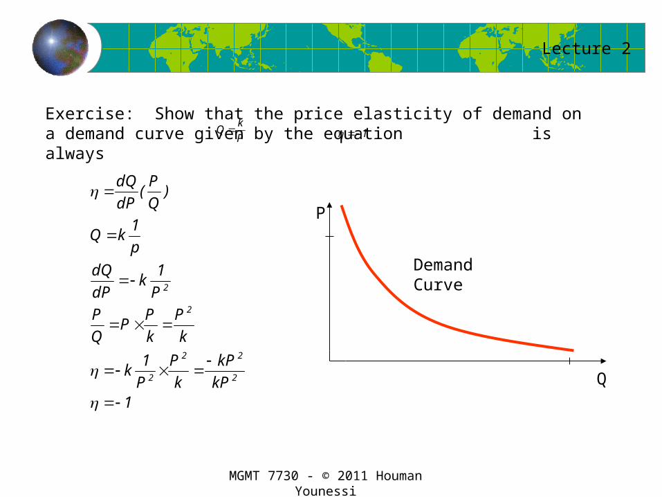
Exercise: Show that the price elasticity of demand on a demand curve given by the equation is always P

kQ 1

1

1

1

1

)(

2

22

2

2

2

kP

kP

k

P

Pk

k

P

k

PP

Q

P

Pk

dP

dQ

pkQ

Q

P

dP

dQ

Lecture 2


Exercise: Given the price elasticity of demand and the price, find marginal revenue

1

1

))((1

PMR

dQ

dP

P

QP

dQ

dPQP

dQ

dPQ

dQ

dQP

dQ

dPQ

dQ

dTRMR

PQTR

Lecture 2


Exercise: Given price elasticity of demand and marginal cost, what is the maximum price we should charge?

1

1PMRWe said that:

We also know that in order for price to be maximum, MR=MC, so

MCPMRPfor

1

1max

111

11

MCMCP

or

PMC

is the maximum price you should charge

Lecture 2


Income Elasticity of DemandBy what percentage would the quantity demanded change as a result of one unit of change in consumer income?

The percentage change of quantity would be:

The percentage change of income would be:

Dividing one by the other:

Q

Q

I

I

I

I

Q

Q

Rearranging:I

Q

Q

IE

)(

dI

dQ

I

Q

I

Q

Q

IE

)(

dI

dQ

Q

II )(Therefore: becomes

At the limit:

Lecture 2


Given that: Q= -700P+200I-500S+0.01A

Example:

Determine the income elasticity of demand for laptops in 2007 when Income is $33000

200dI

dQ

S=$400 P=$3000 and A=$50,000,000

dI

dQ

Q

II )(

375.12004800000

33000)( dI

dQ

Q

II

Therefore one percent increase in income leads to 1.375 percent increase in demand for laptops.

Lecture 2


Cross Elasticity of DemandBy what percentage would the quantity demanded change as a result of one unit of change in the price of an associated product?

Y

X

X

YXY dP

dQ

Q

P)(

Example:

Determine the cross elasticity of demand for laptops in 2007 when price of software is $400

042.05004800000

400)(

Y

X

X

YXY dP

dQ

Q

P

Therefore one percent increase in price of software leads to 0.042 percent decrease in demand for laptops.

Documents

Lecture 2 MGMT 7730 - © 2011 Houman Younessi Derivatives Derivative of a constant Y X Y=3 Y1 X1X2