Lecture 2: Linear Perturbation Theory - University of …background.uchicago.edu/~whu/Presentations/trieste_print2.pdf · Lecture 2: Linear Perturbation Theory Wayne Hu Trieste,

Lecture 2: Linear Perturbation Theory

Wayne HuTrieste, June 2002

Structure Formationand the

Dark Sector

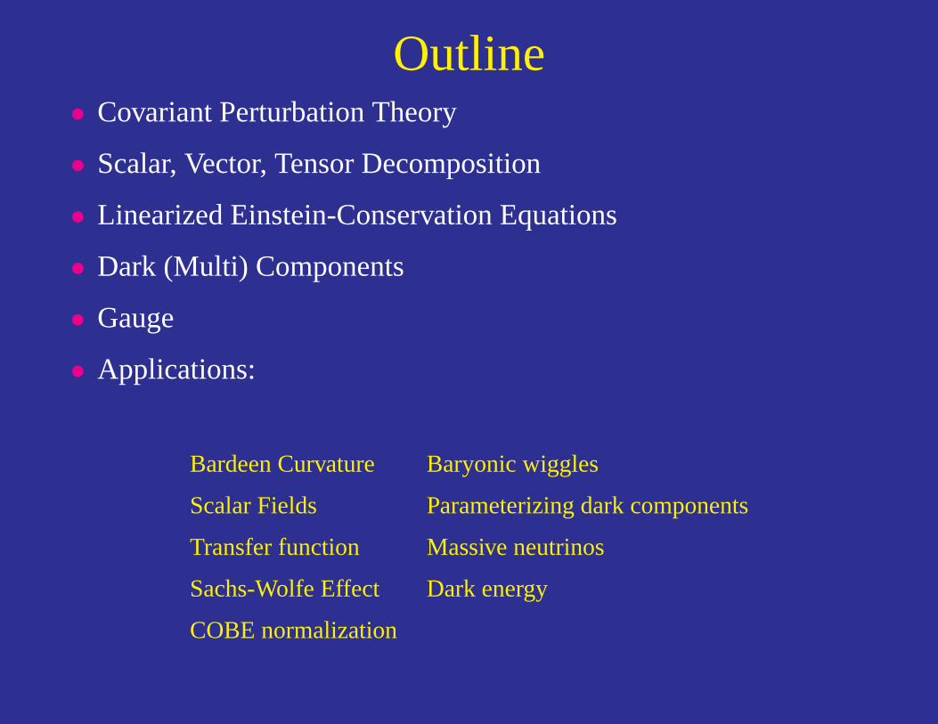
Outline• Covariant Perturbation Theory

• Scalar, Vector, Tensor Decomposition

• Linearized Einstein-Conservation Equations

• Dark (Multi) Components

• Gauge

• Applications:

Bardeen Curvature Baryonic wiggles

Scalar Fields Parameterizing dark components

Transfer function Massive neutrinos

Sachs-Wolfe Effect Dark energy

COBE normalization

Covariant Perturbation Theory• Covariant= takes sameform in all coordinate systems

• Invariant= takes the samevaluein all coordinate systems

• Fundamental equations:Einstein equations, covariantconservationof stress-energy tensor:

Gµν = 8πGTµν

∇µTµν = 0

• Preserve general covariance by keeping alldegrees of freedom: 10for each symmetric 4×4 tensor

1 2 3 45 6 7

8 910

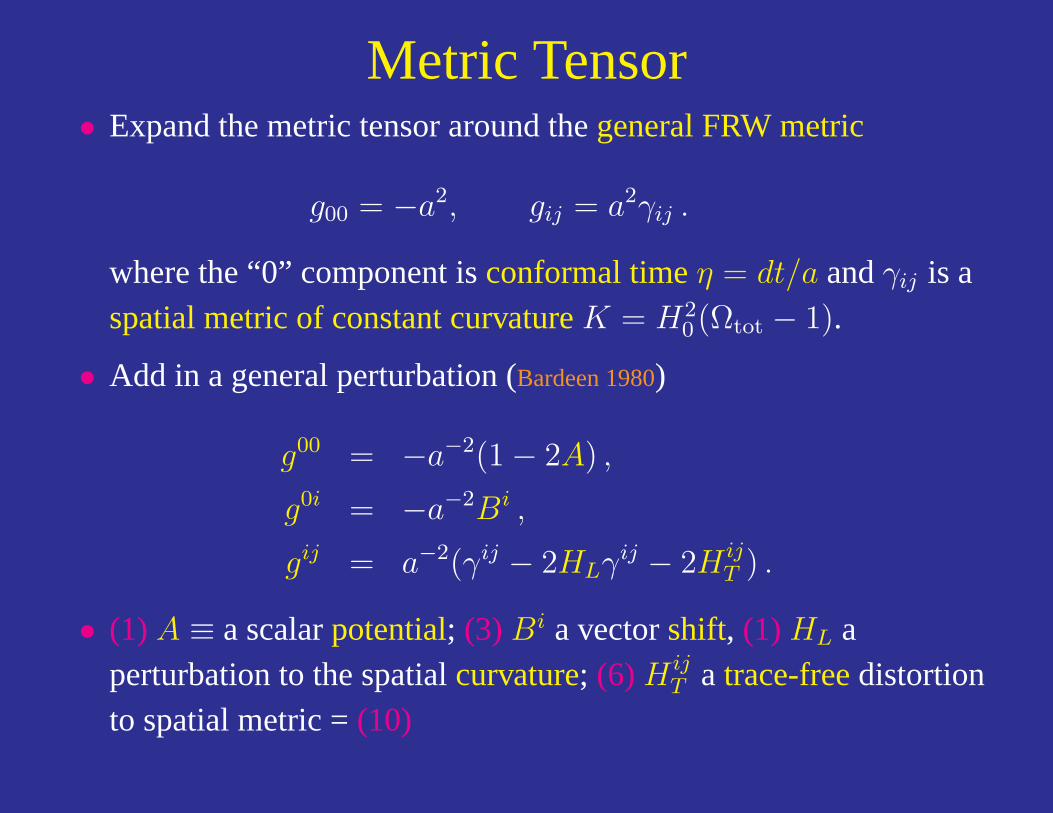
Metric Tensor• Expand the metric tensor around thegeneral FRW metric

g00 = −a2, gij = a2γij .

where the “0” component isconformal timeη = dt/a andγij is aspatial metric of constant curvatureK = H2

0 (Ωtot − 1).

• Add in a general perturbation (Bardeen 1980)

g00 = −a−2(1− 2A) ,

g0i = −a−2Bi ,

gij = a−2(γij − 2HLγij − 2H ijT ) .

• (1) A ≡ a scalarpotential; (3) Bi a vectorshift, (1) HL aperturbation to the spatialcurvature; (6) H ij

T a trace-freedistortionto spatial metric =(10)

Matter Tensor• Likewise expand the matterstress energytensor around a

homogeneous densityρ and pressurep:

T 00 = −ρ− δρ ,

T 0i = (ρ + p)(vi −Bi) ,

T i0 = −(ρ + p)vi ,

T ij = (p + δp)δi

j + pΠij ,

• (1) δρ adensity perturbation; (3) vi a vectorvelocity, (1) δp apressure perturbation; (5) Πij ananisotropic stressperturbation

• So far this isfully generaland applies to any type of matter orcoordinate choice including non-linearities in the matter, e.g.cosmological defects.

Counting DOF’s

20 Variables (10 metric; 10 matter)

−10 Einstein equations

−4 Conservation equations

+4 Bianchi identities

−4 Gauge (coordinate choice 1 time, 3 space)

——

6 Degrees of freedom

• Without loss of generality these can be taken to be the6componentsof thematter stress tensor

• For the background, specifyp(a) or equivalentlyw(a) ≡ p(a)/ρ(a) theequation of stateparameter.

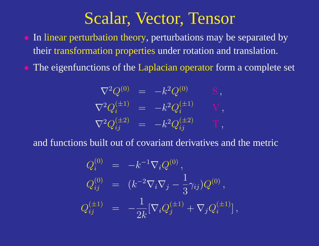
Scalar, Vector, Tensor• In linear perturbation theory, perturbations may be separated by

their transformation propertiesunder rotation and translation.

• The eigenfunctions of theLaplacian operatorform a complete set

∇2Q(0) = −k2Q(0) S ,

∇2Q(±1)i = −k2Q

(±1)i V ,

∇2Q(±2)ij = −k2Q

(±2)ij T ,

and functions built out of covariant derivatives and the metric

Q(0)i = −k−1∇iQ

(0) ,

Q(0)ij = (k−2∇i∇j −

1

3γij)Q

(0) ,

Q(±1)ij = − 1

2k[∇iQ

(±1)j +∇jQ

(±1)i ] ,

Spatially Flat Case• For a spatially flat background metric, harmonics are related to

plane waves:

Q(0) = exp(ik · x)

Q(±1)i =

−i√2(e1 ± ie2)iexp(ik · x)

Q(±2)ij = −

√3

8(e1 ± ie2)i(e1 ± ie2)jexp(ik · x)

wheree3 ‖ k.

• For vectors, the harmonic points in a direction orthogonal tok

suitable for thevortical componentof a vector

• For tensors, the harmonic is transverse and traceless as appropriatefor the decompositon ofgravitational waves

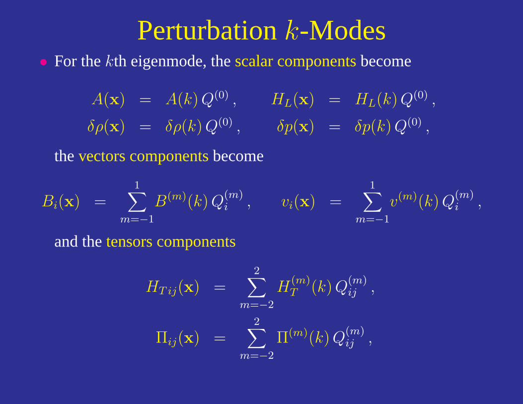
Perturbationk-Modes• For thekth eigenmode, thescalar componentsbecome

A(x) = A(k) Q(0) , HL(x) = HL(k) Q(0) ,

δρ(x) = δρ(k) Q(0) , δp(x) = δp(k) Q(0) ,

thevectors componentsbecome

Bi(x) =1∑

m=−1

B(m)(k) Q(m)i , vi(x) =

1∑m=−1

v(m)(k) Q(m)i ,

and thetensors components

HT ij(x) =2∑

m=−2

H(m)T (k) Q

(m)ij ,

Πij(x) =2∑

m=−2

Π(m)(k) Q(m)ij ,

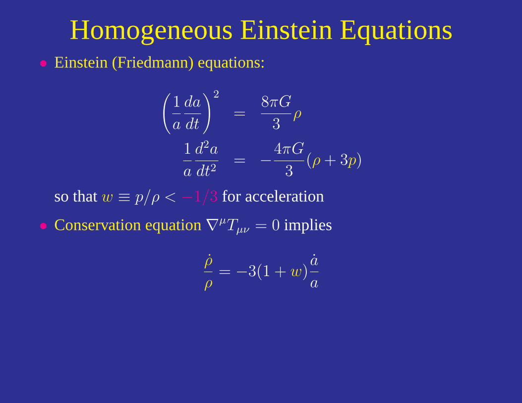
Homogeneous Einstein Equations• Einstein (Friedmann) equations:

(1

a

da

dt

)2

=8πG

3ρ

1

a

d2a

dt2= −4πG

3(ρ + 3p)

so thatw ≡ p/ρ < −1/3 for acceleration

• Conservation equation∇µTµν = 0 implies

ρ

ρ= −3(1 + w)

a

a

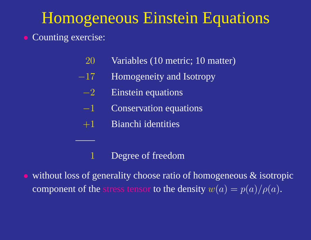
Homogeneous Einstein Equations• Counting exercise:


−17 Homogeneity and Isotropy




——

1 Degree of freedom

• without loss of generality choose ratio of homogeneous & isotropiccomponent of thestress tensorto the densityw(a) = p(a)/ρ(a).

Covariant Scalar Equations• Einstein equations(suppressing0) superscripts (Hu & Eisenstein 1999):

(k2 − 3K)[HL +13HT +

a

a

1k2

(kB − HT )]

= 4πGa2

[δρ + 3

a

a(ρ + p)(v −B)/k

], Poisson Equation

k2(A + HL +13HT ) +

(d

dη+ 2

a

a

)(kB − HT )

= 8πGa2pΠ ,

a

aA− HL −

13HT −

K

k2(kB − HT )

= 4πGa2(ρ + p)(v −B)/k ,[2a

a− 2

(a

a

)2

+a

a

d

dη− k2

3

]A−

[d

dη+

a

a

](HL +

13kB)

= 4πGa2(δp +13δρ) .

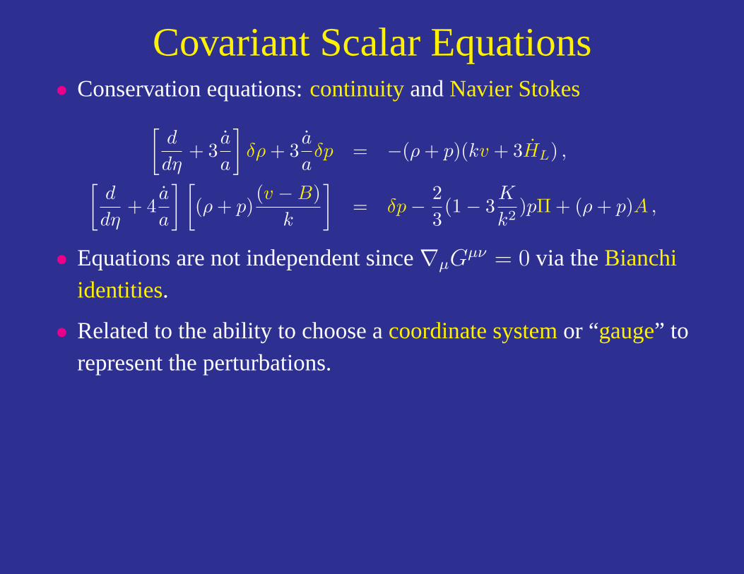
Covariant Scalar Equations• Conservation equations:continuityandNavier Stokes[

d

dη+ 3

a

a

]δρ + 3

a

aδp = −(ρ + p)(kv + 3HL) ,[

d

dη+ 4

a

a

] [(ρ + p)

(v −B)k

]= δp− 2

3(1− 3

K

k2)pΠ + (ρ + p)A ,

• Equations are not independent since∇µGµν = 0 via theBianchi

identities.

• Related to the ability to choose acoordinate systemor “gauge” torepresent the perturbations.

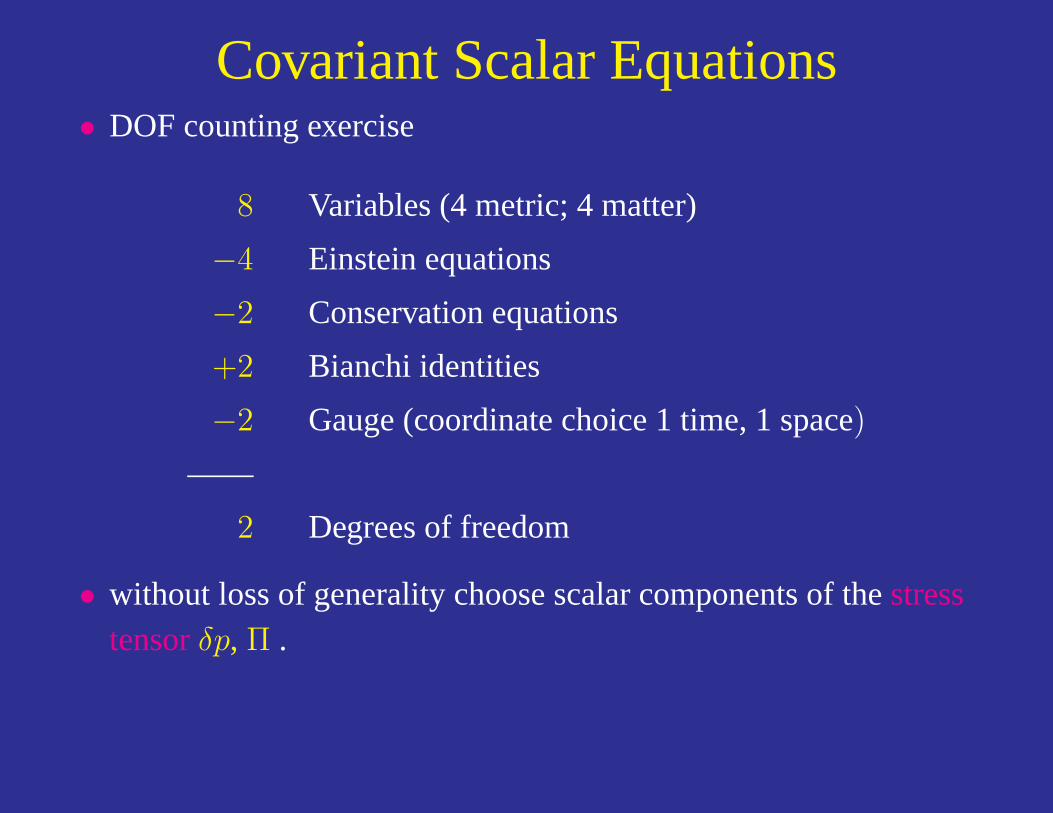
Covariant Scalar Equations• DOF counting exercise






——


• without loss of generality choose scalar components of thestresstensorδp, Π .

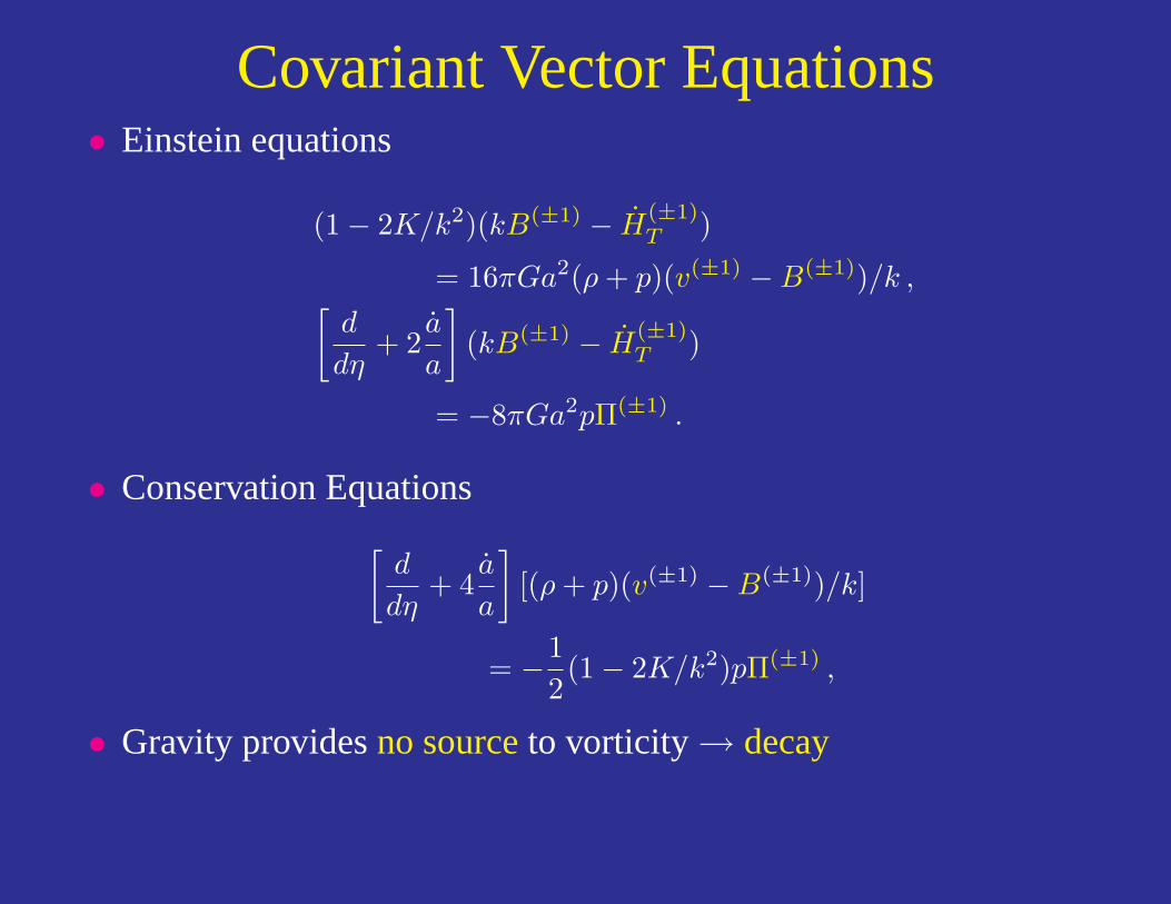
Covariant Vector Equations• Einstein equations

(1− 2K/k2)(kB(±1) − H(±1)T )

= 16πGa2(ρ + p)(v(±1) −B(±1))/k ,[d

dη+ 2

a

a

](kB(±1) − H

(±1)T )

= −8πGa2pΠ(±1) .

• Conservation Equations[d

dη+ 4

a

a

][(ρ + p)(v(±1) −B(±1))/k]

= −12(1− 2K/k2)pΠ(±1) ,

• Gravity providesno sourceto vorticity→ decay

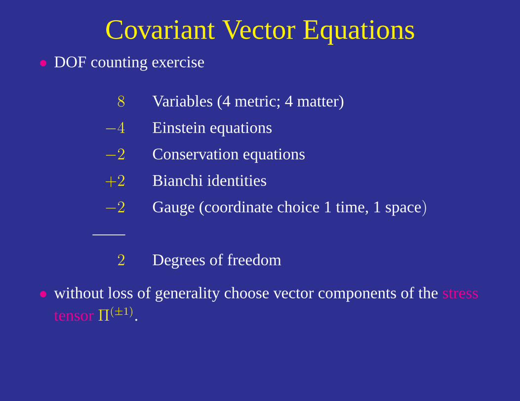
Covariant Vector Equations• DOF counting exercise






——


• without loss of generality choose vector components of thestresstensorΠ(±1).

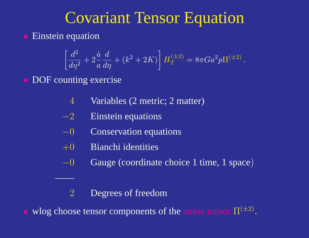
Covariant Tensor Equation• Einstein equation[

d2

dη2+ 2

a

a

d

dη+ (k2 + 2K)

]H

(±2)T = 8πGa2pΠ(±2) .

• DOF counting exercise






——


• wlog choose tensor components of thestress tensorΠ(±2).

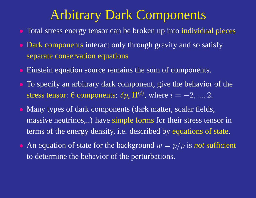
Arbitrary Dark Components• Total stress energy tensor can be broken up intoindividual pieces

• Dark componentsinteract only through gravity and so satisfyseparate conservation equations

• Einstein equation source remains the sum of components.

• To specify an arbitrary dark component, give the behavior of thestress tensor: 6 components: δp, Π(i), wherei = −2, ..., 2.

• Many types of dark components (dark matter, scalar fields,massive neutrinos,..) havesimple formsfor their stress tensor interms of the energy density, i.e. described byequations of state.

• An equation of state for the backgroundw = p/ρ is notsufficientto determine the behavior of the perturbations.

Gauge• Metric and matter fluctuations take ondifferent valuesin different

coordinate system

• No such thing as a “gauge invariant” density perturbation!

• Generalcoordinate transformation:

η = η + T

xi = xi + Li

free to choose(T, Li) to simplify equations or physics.Decompose these into scalar and vector harmonics.

• Gµν andTµν transform astensors, so components in differentframes can be related

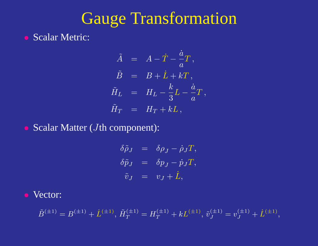
Gauge Transformation• Scalar Metric:

A = A− T − a

aT ,

B = B + L + kT ,

HL = HL −k

3L− a

aT ,

HT = HT + kL ,

• Scalar Matter (J th component):

δρJ = δρJ − ρJT ,

δpJ = δpJ − pJT ,

vJ = vJ + L,

• Vector:

B(±1) = B(±1) + L(±1), H(±1)T = H

(±1)T + kL(±1), v

(±1)J = v

(±1)J + L(±1),

Gauge Dependence of Density Background evolution of the density induces a density fluctuation

from a shift in the time coordinate•

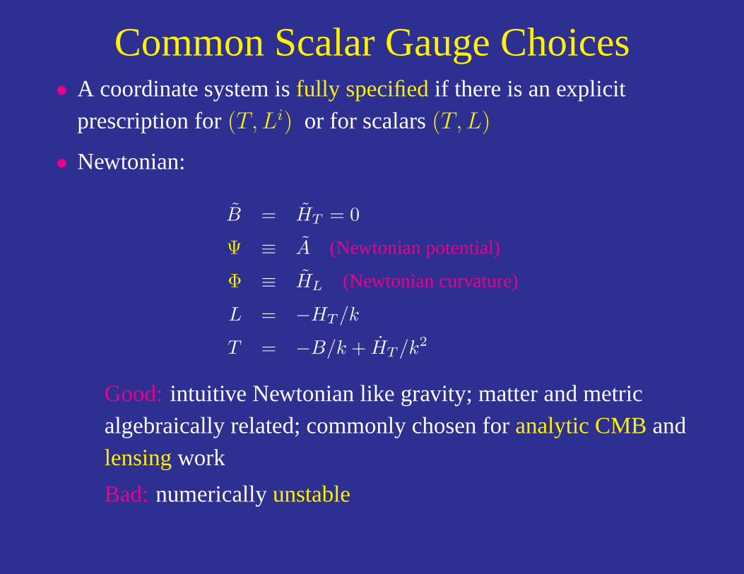
Common Scalar Gauge Choices• A coordinate system isfully specifiedif there is an explicit

prescription for(T, Li) or for scalars(T, L)

• Newtonian:

B = HT = 0

Ψ ≡ A (Newtonian potential)

Φ ≡ HL (Newtonian curvature)

L = −HT /k

T = −B/k + HT /k2

Good:intuitive Newtonian like gravity; matter and metricalgebraically related; commonly chosen foranalytic CMBandlensingwork

Bad: numericallyunstable

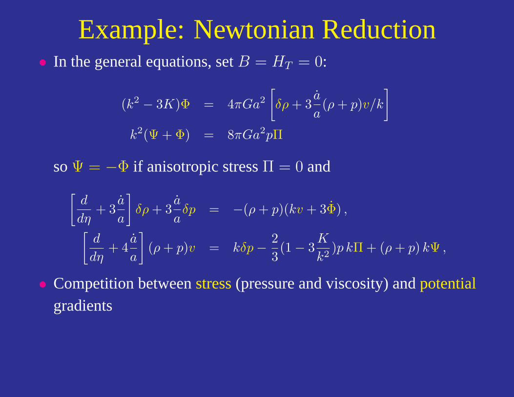
Example: Newtonian Reduction• In the general equations, setB = HT = 0:

(k2 − 3K)Φ = 4πGa2

[δρ + 3

a

a(ρ + p)v/k

]k2(Ψ + Φ) = 8πGa2pΠ

soΨ = −Φ if anisotropic stressΠ = 0 and[d

dη+ 3

a

a

]δρ + 3

a

aδp = −(ρ + p)(kv + 3Φ) ,[

d

dη+ 4

a

a

](ρ + p)v = kδp− 2

3(1− 3

K

k2)p kΠ + (ρ + p) kΨ ,

• Competition betweenstress(pressure and viscosity) andpotentialgradients

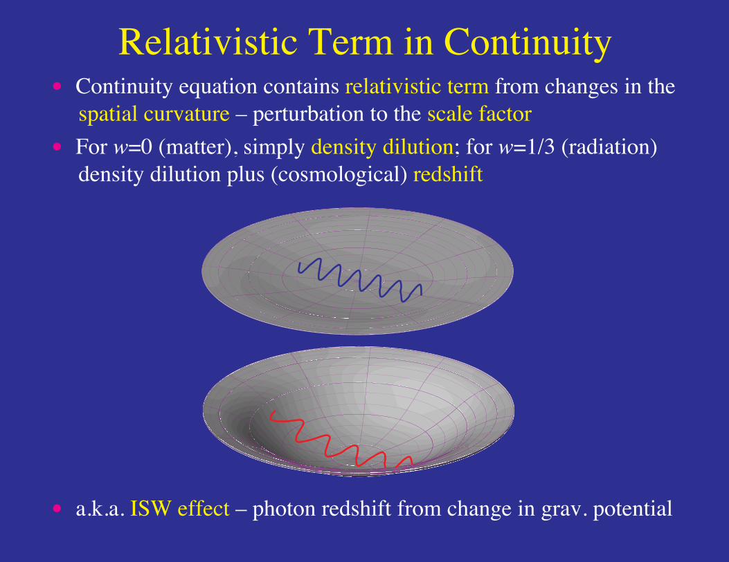
Relativistic Term in Continuity• Continuity equation contains relativistic term from changes in the spatial curvature – perturbation to the scale factor• For w=0 (matter), simply density dilution; for w=1/3 (radiation) density dilution plus (cosmological) redshift

• a.k.a. ISW effect – photon redshift from change in grav. potential

Common Scalar Gauge Choices• Comoving:

B = v (T 0i = 0)

HT = 0

ξ = A

ζ = HL (Bardeen curvature)

T = (v −B)/k

L = −HT /k

Good:ζ is conservedif stress fluctuations negligible, e.g. abovethe horizon if|K| H2

ζ + Kv/k =a

a

[− δp

ρ + p+

23

(1− 3K

k2

)p

ρ + pΠ

]→ 0

Bad: explicitly relativistic choice

Common Scalar Gauge Choices• Synchronous:

A = B = 0

ηL ≡ −HL −13HT

hT = HT or h = 6HL

T = a−1

∫dηaA + c1a

−1

L = −∫

dη(B + kT ) + c2

Good:stable, the choice of numerical codes

Bad: residualgauge freedomin constantsc1, c2 must bespecified as an initial condition, intrinsically relativistic.

Common Scalar Gauge Choices• Spatially Unperturbed:

HL = HT = 0

L = −HT /k

A , B = metric perturbations

T =(

a

a

)−1 (HL +

13HT

)Good:eliminates spatial metric in evolution equations; useful ininflationary calculations(Mukhanov et al)

Bad: intrinsically relativistic.

• Caution:perturbation evolution is governed by the behavior ofstress fluctuations and an isotropic stress fluctuationδp is gaugedependent.

Hybrid “Gauge Invariant” Approach• With the gauge transformation relations, express variables ofone

gaugein terms of those inanother– allows a mixture in theequations of motion

• Example:Newtonian curvature above the horizon. Conservation ofthe Bardeen-curvatureζ=const. implies:

Φ =3 + 3w

5 + 3wζ

e.g. calculateζ from inflation determinesΦ for any choice ofmatter content or causal evolution.

• Example:Scalar field (“quintessence” dark energy) equations incomoving gauge imply asound speedδp/δρ = 1 independent ofpotentialV (φ). Solve in synchronous gauge (Hu 1998).

Transfer Function Example• Example:Transfer functiontransfers the initial Newtonian

curvature to its value today (linear response theory)

T (k) =Φ(k, a = 1)

Φ(k, ainit)

• Conservation of Bardeen curvature: Newtonian curvature is aconstantwhenstress perturbations are negligible: above thehorizon during radiation and dark energy domination, on all scalesduring matter domination

• When stress fluctuations dominate, perturbations are stabilized bytheJeans mechanism

• Hybrid Poisson equation: Newtonian curvature, comoving densityperturbation∆ ≡ (δρ/ρ)com impliesΦ decays

(k2 − 3K)Φ = 4πGρ∆ ∼ η−2∆

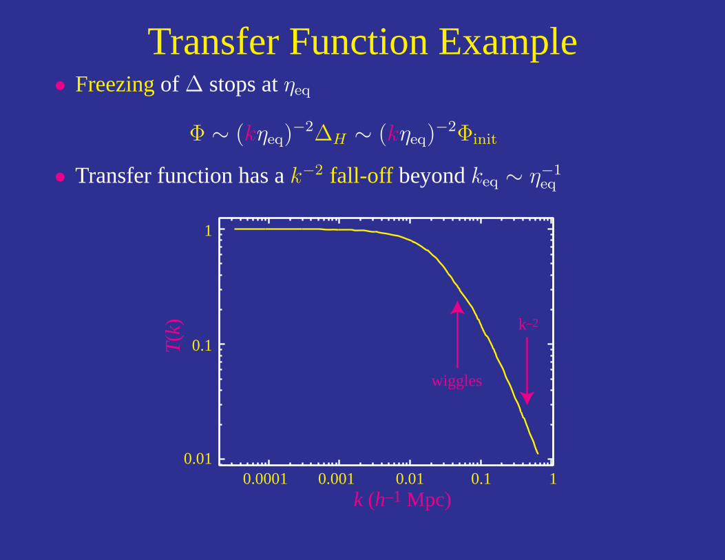
Transfer Function Example• Freezingof ∆ stops atηeq

Φ ∼ (kηeq)−2∆H ∼ (kηeq)

−2Φinit

• Transfer function has ak−2 fall-off beyondkeq ∼ η−1eq

1

0.1

0.0001 0.001 0.01 0.1 10.01

T(k)

k (h–1 Mpc)

wiggles

k–2

Gauge and the Sachs-Wolfe Effect• Going fromcomoving gauge, where the CMB temperature

perturbation is initially negligible by the Poisson equation, to theNewtoniangauge involves a temporal shift

δt

t= Ψ

• Temporal shift implies a shift in thescale factorduring matterdomination

δa

a=

2

3

δt

t

• CMB temperature iscoolingasT ∝ a

• Inducedtemperature fluctuation

δT

T= −δa

a= −2

3Ψ

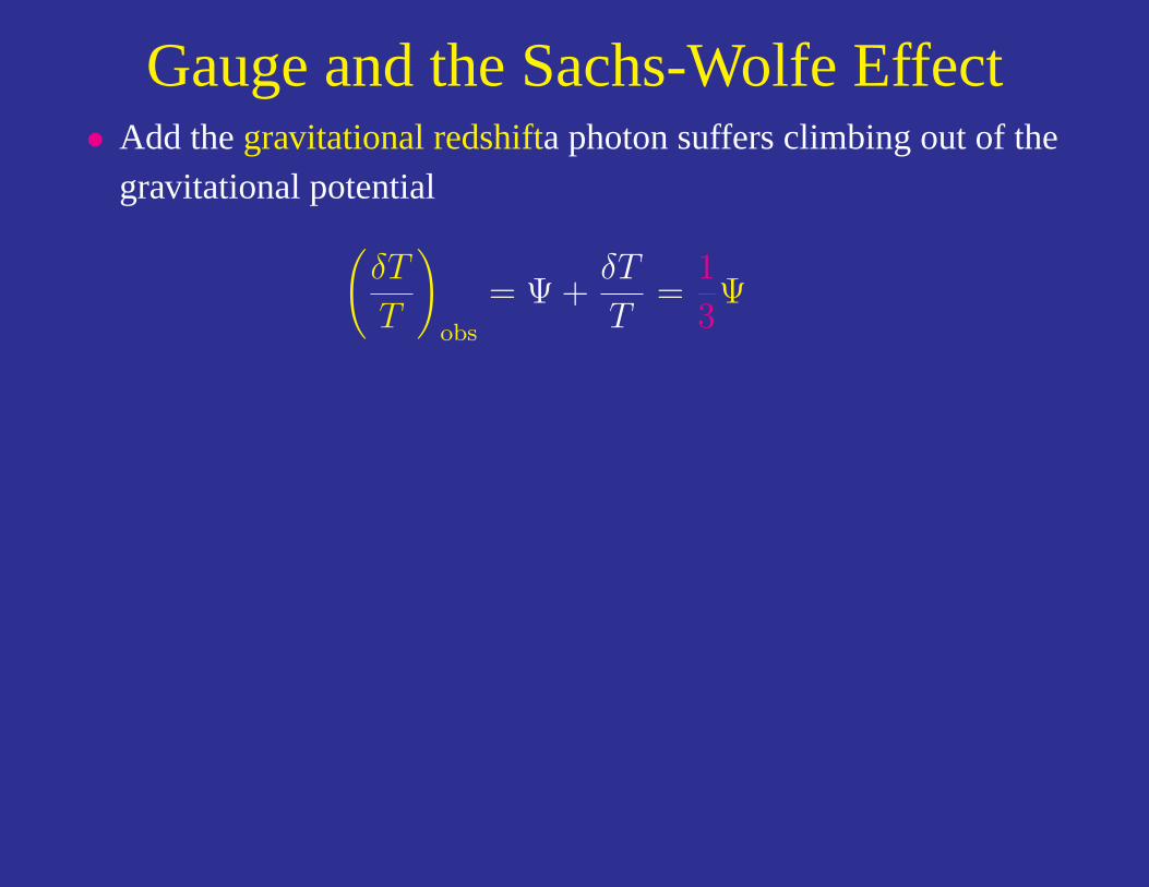
Gauge and the Sachs-Wolfe Effect• Add thegravitational redshifta photon suffers climbing out of the

gravitational potential(δT

T

)obs

= Ψ +δT

T=

1

3Ψ

COBE Normalization

•Sachs-Wolfe Effect relates the COBE detection to the gravitational potential on the last scattering surface

•Decompose the angular and spatial information into normal modes: spherical harmonics for angular, plane waves for spatial

Gm` (n,x,k) = (−i)`

√4π

2` + 1Y m

` (n)eik·x .

x,

D

jl(kD)Yl0

[Θ + Ψ](n,x) =1

3Ψ x + Dn, η∗)

D = η0 − η

(

Last Scattering Surface

η∗

η0

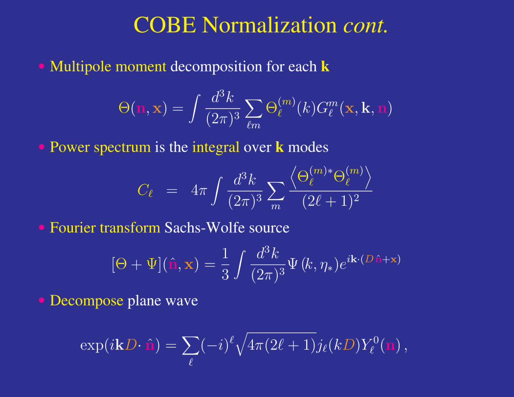
COBE Normalization cont.

•Multipole moment decomposition for each k

•Power spectrum is the integral over k modes

•Fourier transform Sachs-Wolfe source

•Decompose plane wave

Θ(n,x) =∫

d3k

(2π)3

∑`m

Θ(m)` (k)Gm

` (x,k,n)

C` = 4π∫

d3k

(2π)3

∑m

⟨Θ

(m)∗` Θ

(m)`

⟩(2` + 1)2

[Θ + Ψ](n,x) =1

3

∫d3k

(2π)3Ψ k, η∗)e

ik·(D n+x)(

exp(ikD· n) =∑

`

(−i)`√

4π(2` + 1)j`(kD)Y 0` (n) ,


•Extract multipole moment, assume a constant potential

•Construct angular power spectrum

•For scale invariant potential (n=1), integral reduces to

•Log power spectrum = Log potential spectrum / 9

Θ(0)`

2` + 1=

1

3Ψ k, η∗)j`(kD)

=1

3Ψ k, η0)j`(kD)

(

(

C` = 4π∫

dk

kj2` (kD)

1

9∆2

Ψ

∫ ∞

0

dx

xj2` (x) =

1

2`(` + 1)

`(` + 1)

2πC` =

1

9∆2

Ψ (n = 1)


•Relate to density fluctuations: Poisson equation and Friedmann eqn.

•Power spectra relation

•In terms of density fluctuation at horizon and transfer function

•For scale invariant potential

k2Ψ −4πGa2δρ

= −3

2H2

0Ω2mδ

∆2Ψ =

9

4

(H0

k

)4

Ω2m∆2

δ

∆2δ ≡ δ2

H

k

H0

n+3

T 2(k)

`(` + 1)

2πC` =

1

4Ω2

mδ2H (n = 1)

=

( )


•Some numbers

•Detailed calculation from Bunn & White (1997) including decay of potential in low density universe and tilt

`(` + 1)

2πC` =

1

4Ω2

mδ2H (n = 1)

=

28µK

2.726 × 106µK

)2

≈ 10−10

δH ≈ (2 × 10−5)Ω−1m

)

δH = 1.94 × 10−5Ω−0.785−0.05 lnΩmm e−0.95(n−1)−0.169(n−1)2

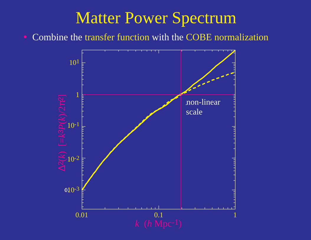
Matter Power Spectrum Combine the transfer function with the COBE normalization•

k (h Mpc-1)

∆2(k

) [=

k3P(

k)/2

π2]

0.1 10.01

1

10-2

101

10-1

10-3

nonon-linearscale

Matter Power Spectrum Usually plotted as the power spectrum, not log-power spectrum•

k (h Mpc-1)

P(k)

(h-

1 M

pc)3

0.1 10.01

103

104

105

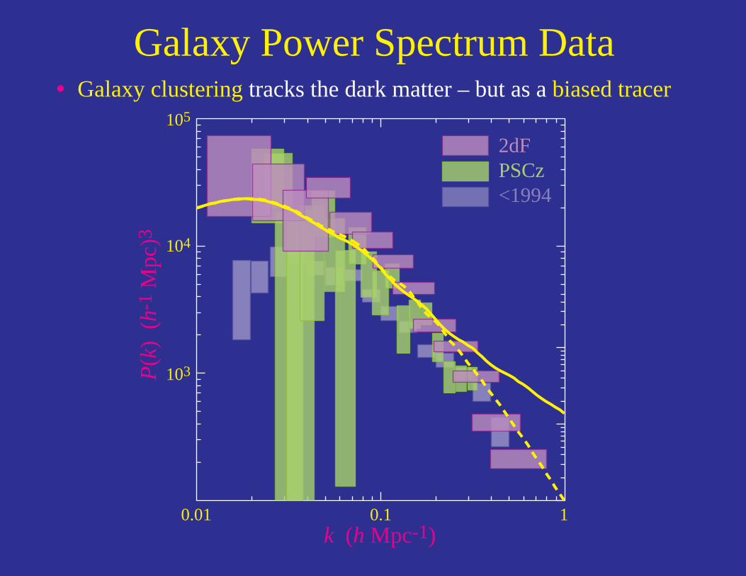
Galaxy Power Spectrum Data Galaxy clustering tracks the dark matter – but as a biased tracer•

k (h Mpc-1)

P(k)

(h-

1 M

pc)3

0.1 10.01

103

104

105

2dFPSCz<1994

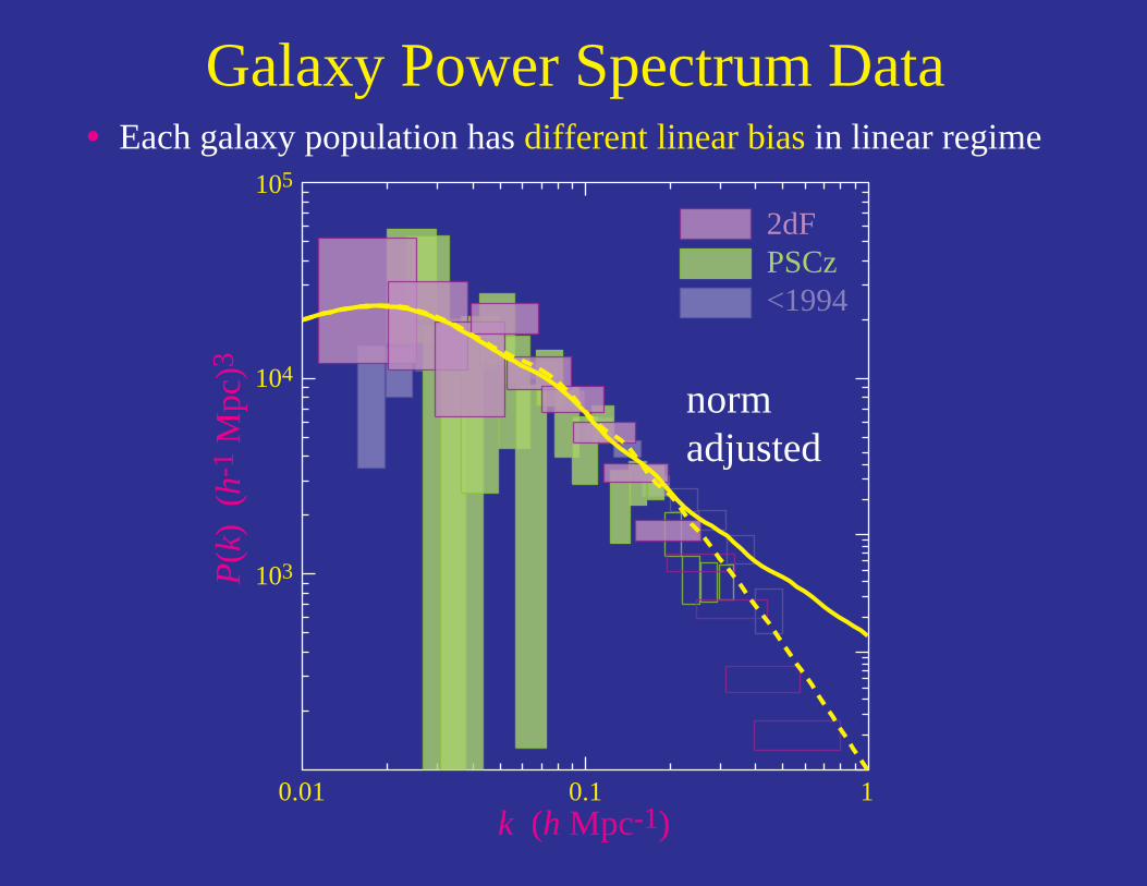
Galaxy Power Spectrum Data Each galaxy population has different linear bias in linear regime•

k (h Mpc-1)

P(k)

(h-

1 M

pc)3

0.1 10.01

103

104

105

2dFPSCz<1994

normadjusted

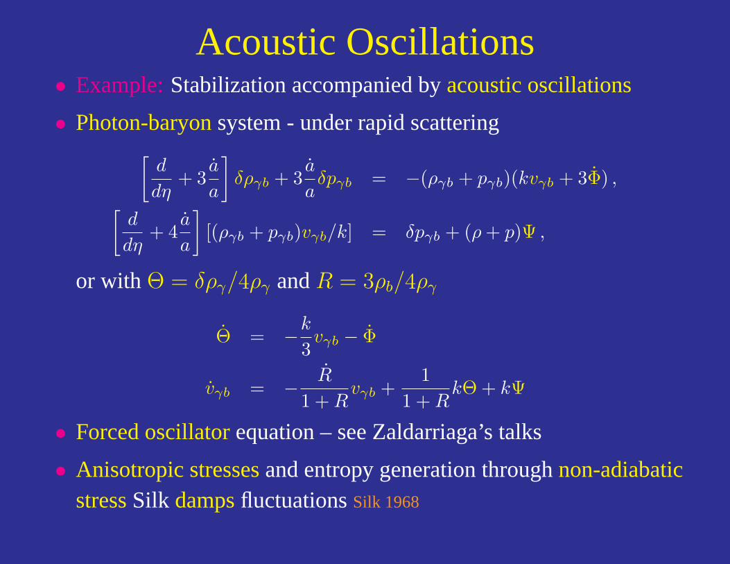
Acoustic Oscillations• Example:Stabilization accompanied byacoustic oscillations

• Photon-baryonsystem - under rapid scattering[d

dη+ 3

a

a

]δργb + 3

a

aδpγb = −(ργb + pγb)(kvγb + 3Φ) ,[

d

dη+ 4

a

a

][(ργb + pγb)vγb/k] = δpγb + (ρ + p)Ψ ,

or with Θ = δργ/ργ and R = 3ρb/ργ

Θ = −k

3vγb − Φ

vγb = − R

1 + Rvγb +

11 + R

kΘ + kΨ

• Forced oscillatorequation – see Zaldarriaga’s talks

• Anisotropic stressesand entropy generation throughnon-adiabaticstressSilk dampsfluctuationsSilk 1968

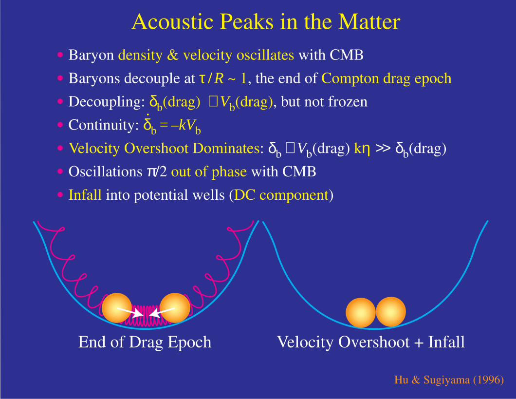
Acoustic Peaks in the Matter• Baryon density & velocity oscillates with CMB

• Baryons decouple at τ / R ~ 1, the end of Compton drag epoch

• Decoupling: δb(drag) ∼ Vb(drag), but not frozen

• Continuity: δb = –kVb

• Velocity Overshoot Dominates: δb ∼ Vb(drag) kη >> δb(drag)

• Oscillations π/2 out of phase with CMB

• Infall into potential wells (DC component)

.

End of Drag Epoch Velocity Overshoot + Infall

Hu & Sugiyama (1996)

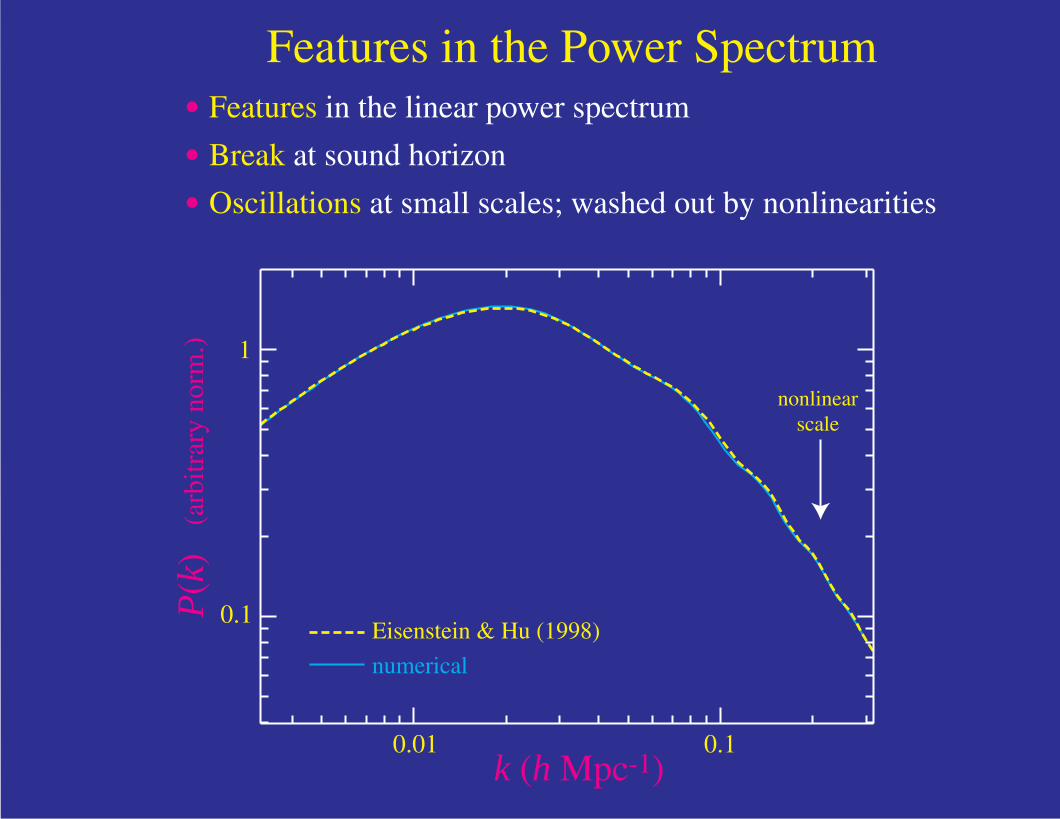
Features in the Power Spectrum• Features in the linear power spectrum

• Break at sound horizon

• Oscillations at small scales; washed out by nonlinearities

k (h Mpc-1)

Eisenstein & Hu (1998)

numerical

P(k

) (

arbi

trar

y no

rm.)

0.01 0.1

0.1

1

nonlinearscale

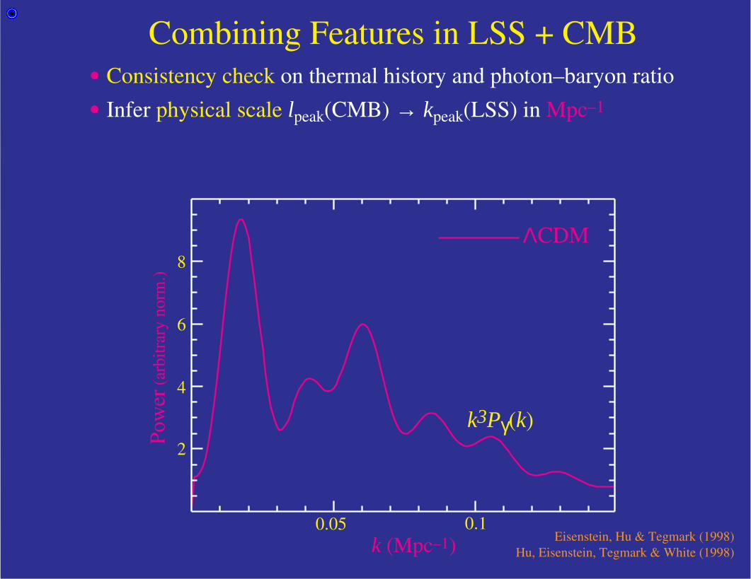
Combining Features in LSS + CMB• Consistency check on thermal history and photon–baryon ratio

• Infer physical scale lpeak(CMB) → kpeak(LSS) in Mpc–1

Eisenstein, Hu & Tegmark (1998)Hu, Eisenstein, Tegmark & White (1998)

k3Pγ(k)

k (Mpc–1)0.05

2

4

6

8

0.1

Pow

er (

arbi

trar

y no

rm.)

ΛCDM

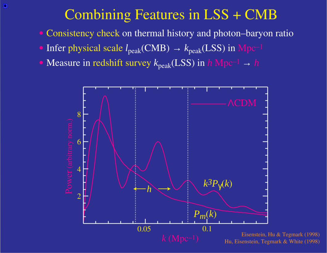
Combining Features in LSS + CMB• Consistency check on thermal history and photon–baryon ratio

• Infer physical scale lpeak(CMB) → kpeak(LSS) in Mpc–1

• Measure in redshift survey kpeak(LSS) in h Mpc–1 → h

Eisenstein, Hu & Tegmark (1998)Hu, Eisenstein, Tegmark & White (1998)

Pm(k)

k3Pγ(k)

k (Mpc–1)0.05

2

4

6

8

0.1

Pow

er (

arbi

trar

y no

rm.)

h

ΛCDM

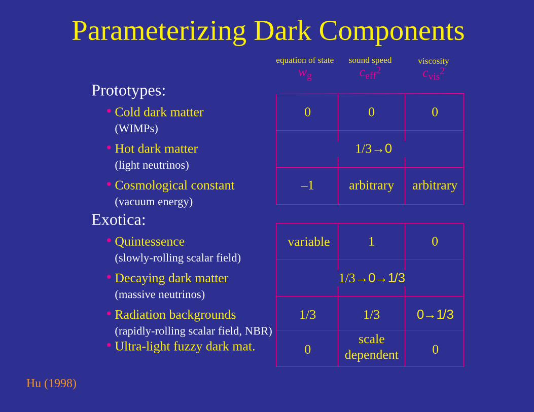
Parameterizing Dark Components

Prototypes:• Cold dark matter 0 0 0

(WIMPs) • Hot dark matter 1/3→0

(light neutrinos)

• Cosmological constant –1 arbitrary arbitrary(vacuum energy)

Exotica:• Quintessence 1 0

(slowly-rolling scalar field)

• Decaying dark matter 1/3→0→1/3(massive neutrinos)

•

•

Radiation backgrounds 1/3

0 0

1/3

scaledependent

0→1/3(rapidly-rolling scalar field, NBR)Ultra-light fuzzy dark mat.

equation of statewg

sound speedceff2

viscositycvis2

variable

Hu (1998)

Massive Neutrinos• Relativisticstressesof a light neutrinoslow thegrowthof structure

• Neutrino species withcosmological abundancecontribute to matterasΩνh

2 = mν/94eV, suppressing power as∆P/P ≈ −8Ων/Ωm

Massive NeutrinosCurrent data from 2dF galaxy survey indicates mν<1.8eVassuming a ΛCDM model with parameters constrained by theCMB.

•

k (h Mpc-1)

P(k)

(h-

1 M

pc)3

0.1 10.01

103

104

105

2dF

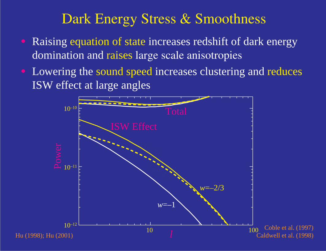
Dark Energy Stress & Smoothness

• Raising equation of state increases redshift of dark energydomination and raises large scale anisotropies

• Lowering the sound speed increases clustering and reducesISW effect at large angles

w=–1

w=–2/3

ceff =1

ceff=1/3

10–10

10–11

10–12

Pow

er

10 100l

ISW Effect

Total

Hu (1998); Hu (2001)Coble et al. (1997)

Caldwell et al. (1998)

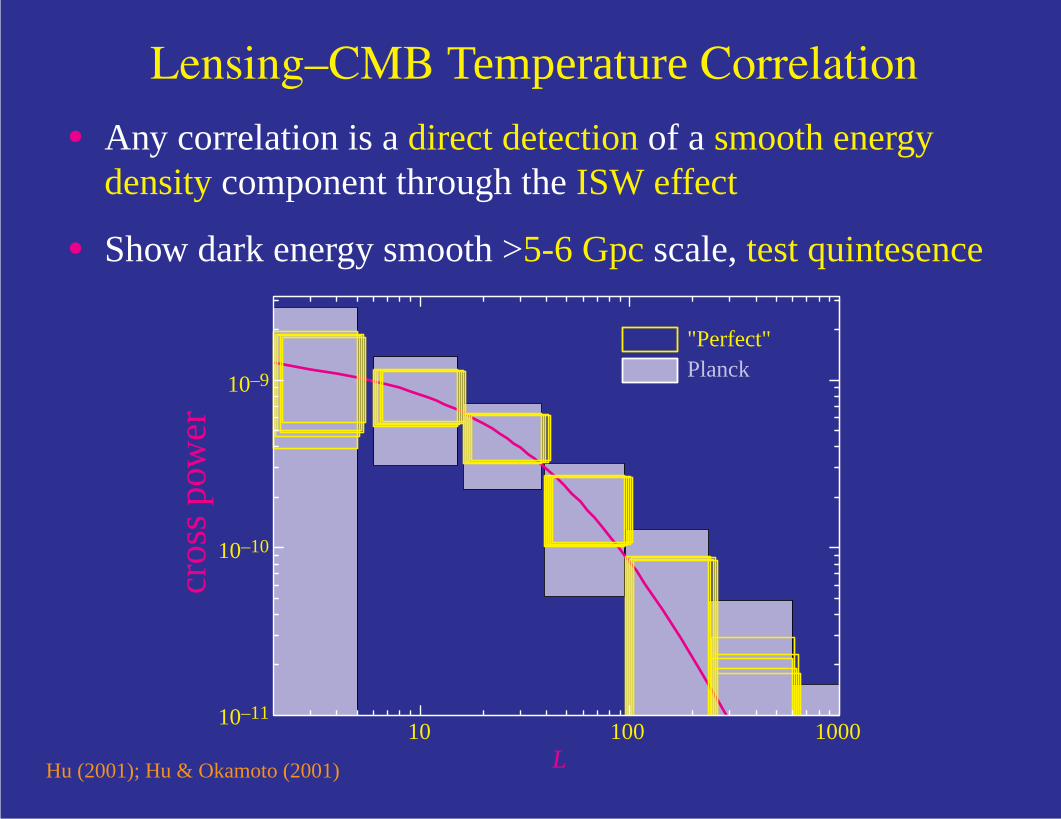
Lensing–CMB Temperature Correlation

• Any correlation is a direct detection of a smooth energy density component through the ISW effect

• Show dark energy smooth >5-6 Gpc scale, test quintesence

Hu (2001); Hu & Okamoto (2001)

10 100 1000

10–9

10–10

10–11

"Perfect"Planck

cros

s po

wer

L

Summary• In linear theory, evolution of fluctuations is completely defined

once thestressesin the matter fields are specified.

• Stresses and their effects take on simple forms in particularcoordinate orgauge choices, e.g. the comoving gauge.

• Gaugecovariant equationscan be used to take advantage of thesesimplifications in an arbitrary frame.

• Curvature(potential) fluctuations remainconstantin the absenceof stresses.

• Evolution can be used to test the nature of thedark components,e.g.massive neutrinosand thedark energyby measuring thematter power spectrum.

• Problem:luminous tracers of the matter clustering arebiased–next lecture.

Documents

Lecture 2: Linear Perturbation Theory - University of …background.uchicago.edu/~whu/Presentations/trieste_print2.pdf · Lecture 2: Linear Perturbation Theory Wayne Hu Trieste,