Lecture 2: Introduction to GLM’s · Lecture 2: Introduction to GLM’s Claudia Czado ... GLM’s allow also to include nonnormal errors such as binomial, Poisson and Gamma errors

c©(Claudia Czado, TU Munich) ZFS/IMS Gottingen 2004 – 0 –

Lecture 2: Introduction to GLM’s

Claudia Czado

TU Munchen


Overview

• Introduction to GLM’s

• Goodness of fit in GLM’s

• Testing in GLM’s

• Estimation in GLM’s


Introduction to GLM’s

In generalized linear models (GLM) we also have independent response variableswith covariates.

While in linear models a good scale of the response variables has to combineadditivity of the covariate effects with the normality of the errors, includingvariance homogeneity, GLM’s don’t need to satisfy these scale requirements.

GLM’s allow also to include nonnormal errors such as binomial, Poisson andGamma errors.

Regression parameters are estimated using maximum likelihood.

The standard reference on GLM’s is McCullagh and Nelder (1989).


Components of a GLM:Response Yi and independent variables Xi = (xi1, · · ·xip) for i = 1, · · · , n.

1. Random Component:Yi, 1 ≤ i ≤ n independent with density from the exponential family, i.e.

f(y; θ, φ) = exp{θy − b(θ)a(φ)

+ c(y, φ)}.

Here φ is a dispersion parameter and functions b(), a() and c(, ) are known.

2. Systematic Component:ηi(β) = xt

iβ = β0 + β1xi1 + · · ·+ βpxip linear predictor,β = (β0, · · · , βp) regression parameters

3. Parametric Link Component:The link function g(µi) = ηi = xt

iβ combines linear predictor with mean µi

of yi. Canonical link function if θ = η.


LM as GLM

Yi = xtiβ + εi = µi + εi, εi ∼ N(0, σ2) iid, i = 1, .., n,

The density of Yi has exponential family form since

f(yi, µi, σ) =1√2πσ

exp{− 1

2σ2(yi − µi)2

}

= exp

yiµi − µ2i2

σ2− 1

2

[ln(2πσ2) +

y2i

σ2

] .

This implies for θi = µi and φ = σ2

b(θi) =µ2

i

2=

θ2i

2, a(φ) = σ2, c(yi, φ) = −1

2

[ln(2πφ) +

y2i

φ

]

Further we have the identity as link function, i.e. g(µi) = µi.


Expectation and variance in GLM’s

When integration and differentiation can be exchanged, mean and variance ina GLM can be represented as

µi = E(Yi) = b′(θi)

V ar(Yi) = a(φ) · b′′(θi).

V (θ) := b′′(θ) is called the variance function of the GLM.


GLM’s implemented in Splus

Distribution Family Link Variance

Normal/Gaussian gaussian µ 1

Binomial binomial ln( µ1−µ) µ(1−µ)

n

Poisson poisson ln(µ) µ

Gamma gamma 1µ µ2

Inverse Normal / inverse.gaussian 1µ2 µ3

GaussianQuasi quasi g(µ) V (µ)

For the binomial family the distribution of Yini

is used. ”Quasi” allows for userdefined GLM’s.


Link functions:

ηi = xtiβ ηi = g(µi) E(Yi) = µi g − monotone ↑

Normal: µi ∈ R, ηi ∈ R.Often g(µ) = µ or for µ > 0

gα(µ) ={

µα−1α α 6= 0

log(µ) α = 0gα(µ) → log(µ), α → 0

Box-Cox - transformation

Poisson: µ > 0, g : R+ → R monotone ↑

g(µ) = log(µ)


Link functions:

Binomial: µ ∈ [0, 1], need g : [0, 1] → R monotone ↑All cdf’s F : R→ [0, 1] monotone ↑ ⇒ g(µ) := F−1(µ)

a) F (z) = ez

1+ez Logit link (symmetric, heavy-tailed)

⇒ g(µ) := F−1(µ) = log(

µ1−µ

)Logistic regression

b) F (z) = Φ(z), Φ(z) = cdf of N(0, 1) Probit Link (symmetric)⇒ g(µ) = Φ−1(µ) Probit regression

c) F (z) = 1− exp{−exp{z}} complementary Log-log distribution⇒ g(µ) = ln(ln(1− µ)) (nonsymmetric)


Canonical link functions

If θi = ηi ∀i holds, we call the corresponding link function canonical.

Examples:

Linear model: θi = µi = ηi ⇒ identity link canonical.

Binomial model: θi = log(

µi1−µi

)= ηi ⇒ logistic link canonical

In GLM with canonical link (n∑

i=1

xi1yi, . . . ,n∑

i=1

xipyi) is sufficient for

(β1, . . . , βp)t.


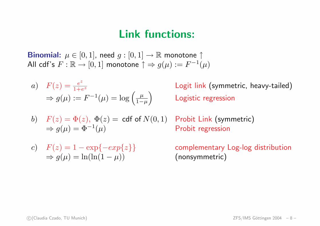
Goodness of fit in GLM: Deviance

Want to estimate Yi by µi.For n data points we can estimate n parameters.

Null model:

µi := Y ∀i, Y :=1n

n∑

i=1

Yi

one parameter → too simple.

Saturated model:µi := Yi ∀i

no error, n parameters used, no explanation of data possible.


Loglikelihood in GLM withηi = g(µi), θi = h(µi) (i = 1, . . . , n)

l(β, φ,y) =n∑

i=1

[yiθi−b(θi)

a(φ) − c(yi, φ)]

=n∑

i=1

[yih(µi)−b(h(µi))

a(φ) − c(yi, φ)]

= l(µ, φ,y) “mean parametrization”

l(µ, φ,y) := log likelihood maximized over µ (φ known) µi := g−1(xitβ)

l(y, φ,y) := log likelihood attainable in saturated model i.e. µi = Yi ∀i

⇒ −2[l(µ, φ,y)− l(y, φ,y)]

= 2n∑

i=1

yi(θi−θi)−b(θi)+b(θi)a(φ) , where θi := h(µi), θi := h(Yi)

If a(φ) = φω ⇒

−2[l(µ, φ,y)− l(y, φ,y)] = 2ωn∑

i=1

yi(θi−θi)−b(θi)+b(θi)φ =: D(y,µ)

φ deviance


Ex: Deviance in Linear and Binomial ModelsLinear model:

l(β, φ,y) = −n∑

i=1

12σ2(yi − µi)2 − n

2 ln(2πσ2), µi = xtiβ, φ = σ2

⇒ −2[l(µ, φ,y)− l(y, φ,y)] = 1σ2

n∑i=1

(Yi − µi)2

⇒ D(y, µ) :=n∑

i=1

(Yi − µi)2

Binomial model:Yi ∼ binomial(ni, pi) independent µi := nipi pi = MLE of pi

D(y, µ) = 2n∑

i=1

{yi ln

(yi

µi

)+ (ni − yi) ln

(ni − yi

ni − µi

)}

In binomial regression models is not {Yi, i = 1, . . . , n} a GLM, but {Yini

, i =1, . . . , n} is a GLM.


Generalized Pearson Statistic

χ2 :=n∑

i=1

(Yi−µi)2

V (µi)

V (µi) = estimated variance function

= b′′(θi)|θi=h(µi)

Examples:Normal: Yi ∼ N(µi, σ

2) ind.

⇒ θi = µi b(µi) = µ2i2 ⇒ b′′(µi) = 1

⇒ χ2 =n∑

i=1

(Yi − µi)2 = D(y, µ).


Logistic Regression: Yi ∼ bin(ni, pi) ind.

pi = eθi

1+eθi⇒ µi = nipi = ni

eθi

1+eθi

b(θi) = ni ln(1 + eθi) ⇒ b′′(θi) = nieθi

(1+eθi)2

⇒ b′′(p) = nipi(1− pi) = µi(1− µin )

⇒ V (µi) = µi(1− µin ) = nipi(1− pi)

⇒ χ2 =n∑

i=1

(yi−nipi)2

nipi(1−pi).


Asymptotic distribution of Deviance and Pearsonstatistic

1) Normal: Y = Xβ + ε X ∈ Rn×p ε ∼ Nn(0, Inσ2)

⇒ D(y, µ) = χ2 =n∑

i=1

(Yi − µi)2 ∼ σ2χ2n−p

2) For all other GLM’s we have

D(y, µ) L→ φχ2n−p, n →∞ p = # of unknown parameters

χ2 L→ φχ2n−p, n →∞

Proof: deviance is equivalent to a likelihood ratio statistic and bχ2 to the Waldstatistic for which general asymptotic results are available (see e.g: Rao (1973))

3) For finite n one has no theoretical results whether D or χ2 is performingbetter.


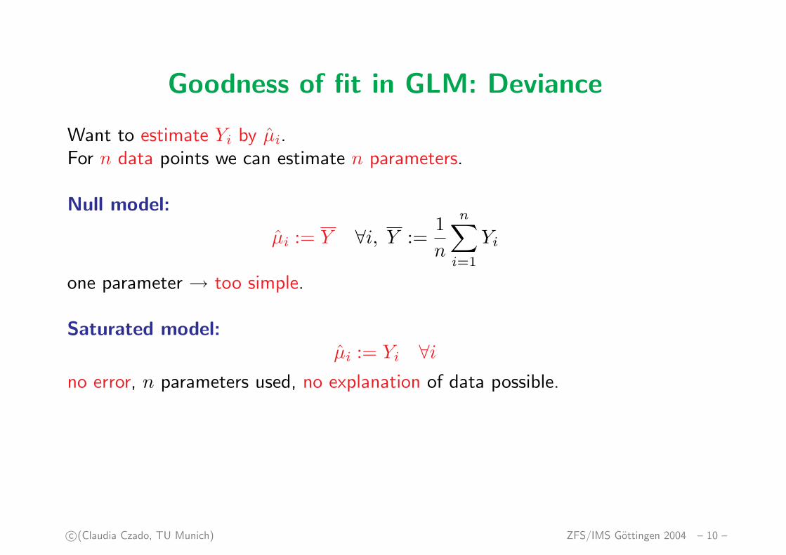
Nested linear models

Model SSE

M1 : Y = 1nβ0 + ε (null model) SSE0

M2 : Y = X1β1 + ε SSE(X1)

M3 : Y = X1β1 + X2β2 + ε (full model) SSE(X1, X2)

X ∈ Rn×p X1 ∈ Rn×p1 X2 ∈ Rn×p2 p1 + p2 = p

Recall: SSE0 =n∑

i=1

(Yi − Y )2

SSE(X1) = ||Y −X1β2

1||2 β2

1 = MLE in M2

SSE(X1, X2) = ||Y −X1β3

1 −X2β3

2||2 β3

1, β3

2 = MLE in M3


Analysis of devianceLet M1 ⊂ M2 ⊂ . . . ⊂ Mr a sequence of nested models with M1 = null modeland Mr = saturated model. That means that all covariates of Mi are containedin Ms for s ≥ i + 1 ∀i.

Model DevianceM1 (null model) Dev1

> Dev1 −Dev2

M2 Dev2... ... ...Mr−1 Devr−1

> Devr−1 −Devr

Mr (saturated model) Devr

-Difference Devi − Devi+1 is considered as the variation explained by Mi+1

minus the variation explained by M1, . . . , Mi. The variations explained byMi+2, . . . , Mr are disregarded.-Analysis of deviance depends on the order of covariates added to the models-Since there is no exact distribution theory, it is used as a screening method toidentify important covariates


Statistical hypothesis testsResidual deviance test

H0 : ηi = g(µi) ∀i H1 : not H0

Reject H0 ⇔ Dev > χ2n−q,1−α is an asymptotic α−level test

Problem: Often one is interested to use this as a goodness-of-fit test, i.e.one wants to accept H0. However the power function is unknown.

Partial deviance test

η = X1β1 + X2β2 Model F with deviance DF β1 ∈ Rp1, β2 ∈ Rp2

η = X1β1 Model R with deviance DR p1 + p2 = p

H0 : β2 = 0 H1 : β2 6= 0

Reject H0 ⇔ DR −DF > χ2p−p2=p1,1−α


Residuals

Pearson residuals: rPi := yi−µi√

V (µi)i = 1, . . . , n

Deviance residuals: rDi := sign(yi − µi)

√di

Dev =n∑

i=1

di di = deviance contribution of ith obs.

sign(x) ={

1 x > 0−1 x ≤ 0

- χ2 =n∑

i=1

(rPi )2, Dev =

n∑i=1

(rDi )2

- For nonnormal GLM Pearson residuals are skewed. Better to use Anscomberesiduals.


Maximum Likelihood Estimation (MLE) in GLM’s

Loglikelihood for obs. i:

li(yi, µi, φ) =[yiθi − b(θi)]

a(φ)+ c(yi, φ)

where g(µi) = ηi µi = E(Yi) = h(θi) ηi = xtiβ β ∈ Rp

Since

∂li∂βj

= ∂li∂µi

dµidηi

∂ηi∂βj

we need

∂ηi∂βj

= xij xi = (xi1, . . . , xip)t

∂li∂µi

= ∂li∂θi

/∂µi∂θi

µi=b′(θi)= yi−b′(θi)a(φ) /b′′(θi) = yi−µi

Vi, since Vi = V ar(Yi) = a(φ) · b′′(θi)

⇒ ∂li∂βj

= ∂li∂µi

dµidηi

∂ηi∂βj

= yi−µiVi

dµidηi

xij


For n independent observations:

l(y, β) :=n∑

i=1

li(yi, µi, φ)

⇒ ∂l∂βj

=n∑

i=1

∂li(yi,µi,φ)∂βj

=n∑

i=1

yi−µiVi

dµidηi

xij Vi = V ar(Yi)

µi = E(Yi)

Let Wi := 1

Vi

(dηidµi

)2 =(

dµidηi

)2

/Vi since dηidµi

= 1/dµidηi

⇒ sj(β) := ∂l(y,β)∂βj

=n∑

i=1

Wi(yi − µi)dηidµi

xij = 0 j = 1, . . . , p

score equations


Newton Raphson Method

Want to solve f(x) =

f1(x1, . . . , xn)...

fn(x1, . . . , xn)

= 0. Let x = ξ the solution and x0

a value close to ξ. Then we have with first order Taylor expansion around x0:

0 = f(ξ) ≈ f(x0) + Df(x0)︸︷︷︸∈Rn×n

(ξ − x0)︸︷︷︸∈Rn

where

Df(x0) :=

∂f1∂x1

· · · ∂f1∂xn... . . . ...

∂fn∂x1

· · · ∂fn∂xn

x=x0⇒ ξ = x0 − [Df(x0)]−1f(x0)

Newton Raphson method is an iterative algorithm with x0 a starting value and

xi+1 = xi − [Df(xi)]−1f(xi)

There are general convergence results available.


To solve s(β) = (s1(β), . . . , sp(β))t = 0 we need

H(β) :=

∂s1∂β1

· · · ∂s1∂βp

... . . . ...∂sp

∂β1· · · ∂sp

∂βp

=

∂2l∂β1∂β1

· · · ∂2l∂β1∂βp

... . . . ...∂2l

∂βp∂β1· · · ∂2l

∂βp∂βp

= Hessian matrix = − observed information matrix

∂2l∂βs∂βr

= ∂∂βs

[n∑

i=1

yi−µiVi

dµidηi

xir

]

=n∑

i=1

(yi − µi) ∂∂βs

[V −1

idµidηi

xir

]+

n∑i=1

V −1i

dµidηi

xir∂

∂βs(yi − µi)

Further ∂∂βs

(yi − µi) = −dµidηi

∂ηi∂βs

= −dµidηi

xis. Since ∂2l∂βs∂βr

depends on Y

in general we use E( ∂2l∂βs∂βr

) instead. Note that for canonical link we have∂2l

∂βs∂βr= E( ∂2l

∂βs∂βr).


Expected information matrix

A(β) :=[−E( ∂2l

∂βs∂βr)]

s,r=1,...,pis called the expected information matrix

One can show that

−E ∂2l∂βs∂βr

= E ∂l∂βs

∂l∂βr

Es(β)=0⇒ A(β) = cov s(β)

The both expressions are used as definition for the expected information matrixin the literature.


Fisher scoring method

E( ∂2l∂βs∂βr

) = E (· · · )︸︷︷︸=0

+E

−

n∑i=1

V −1i

(dµi

dηi

)2

︸︷︷︸Wi

xis xir

= −n∑

i=1

Wi xis xir

⇒ A(β) :=[−E( ∂2l

∂βs∂βr)]

s,r=1,...,p= +XtWX ∈ Rp×p,

where W = diag(W1, . . . , Wn) ∈ Rn×n and X ∈ Rn×p.

Fisher scoring method: let βr the current estimation to the solution ofs(β) = 0, the new estimation value is given by

βr+1 = βr + A−1(βr)s(βr)


Fisher scoring as iterative weighted least squares

Since A(βr)βr+1

︸︷︷︸∈Rp

= A(βr)βr + s(βr)

⇒ (A(βr)βr+1)j =p∑

s=1Ajs(βr)βr

s + sj(βr) g(µri ) = ηr

i = xtiβ

r

=p∑

s=1

n∑i=1

W ri xijxisβ

rs +

n∑i=1

W ri (yi − µr

i )dηr

idµr

ixij

=n∑

i=1

W ri xij [

p∑s=1

xisbrs

︸︷︷︸ηr

i

+(yi − µri )

dηri

dµri]

Define the adjusted dependent variable

Zri := ηr

i + (yi − µri )

dηri

dµri⇒

(A(βr)βr+1)j =n∑

i=1

W ri xijZ

ri


On the other side we have

(A(βr)βr+1)j =p∑

s=1Ajs(βr)βr+1

s =p∑

s=1

n∑i=1

W ri xijxisβ

r+1s

=n∑

i=1

W ri xij

p∑s=1

xisbr+1s

︸︷︷︸ηr+1

i

Therefore we have

n∑

i=1

W ri xijZ

ri =

n∑

i=1

W ri xijη

r+1i ∀j = 1, . . . , p

or in matrix form: XtW rZr = XtW rXβr+1.

These equations correspond to the normal equations of a weighted leastsquares estimation with response Zr

i , covariates x1, . . . ,xp and weights (W ri )−1.

Therefore we speak of the IWLS (iterated weighted least square).


IWLS algorithm

Step 1: Let βr the current estimate of β, determine

- ηri := xi

tβr i = 1, . . . , n (current linear predictors)- µr

i := g−1(ηri ) (current fitted means)

- θri := h−1(µr

i )- V r

i := a(φ) · b′′(θi)|θi=θri

- Zri := ηr

i + (yi − µri )

(dηidµi|ηi=ηr

i

)(adjusted dependent variable)

- W ri :=

[V r

i

(dηidµi|ηi=ηr

i

)2]−1

Step 2: Regress Zri on xi1, . . . , xip with weights (W r

i )−1 to obtain new estimateβr+1 and continue with step 1 until ||βr − βr+1|| sufficiently small.


Remarks1) Zr

i is the linearized form of the link function at yi, since

g(yi) ≈ g(µri )︸︷︷︸

ηri

+(yi − µri ) g′(µr

i )︸︷︷︸dηr

idµr

i⇒ Zri ≈ g(yi) up to the first order

2) V ar(Zri ) ≈ V ar(Yi − µr

i )︸︷︷︸Vi

·(

dηri

dµri

)2

= (W ri )−1

if ηri , µ

ri are considered fixed and known.

3) Often one can use the data as starting values, i.e.

µ0i = yi ⇒ η0

i = g(µ0i )

If Yi = 0 in the binomial case one needs to change the start values to avoidlog(0).


References

McCullagh, P. and J. Nelder (1989). Generalized linear models. Chapman &Hall.

Rao, C. (1973). Linear Statistical Inference and Its Applications, 2nd Ed.New York: Wiley.

Documents

Lecture 2: Introduction to GLM’s · Lecture 2: Introduction to GLM’s Claudia Czado ... GLM’s allow also to include nonnormal errors such as binomial, Poisson and Gamma errors