Lecture 2ESTIMATING THE SURVIVAL

FUNCTION

— One-sample nonparametric methods

There are commonly three methods for estimating a sur-

vivorship function

S(t) = P (T > t)

without resorting to parametric models:

(1) Kaplan-Meier

(2) Nelson-Aalen or Fleming-Harrington (via esti-

mating the cumulative hazard)

(3) Life-table (Actuarial Estimator)

We will mainly consider the first two.

1

(1) The Kaplan-Meier Estimator

The Kaplan-Meier (or KM) estimator is probably the most

popular approach.

Motivation (no censoring):

Remission times (weeks) for 21 leukemia patients receiving

control treatment (Table 1.1 of Cox & Oakes):

1, 1, 2, 2, 3, 4, 4, 5, 5, 8, 8, 8, 8, 11, 11, 12, 12, 15, 17, 22, 23

We estimate S(10), the probability that an individual sur-

vives to week 10 or later, by 821.

How would you calculate the standard error of the estimated

survival?

S(10) = P (T > 10) =8

21= 0.381

(Answer: se[S(10)] = 0.106)

What about S(8)? Is it 1221 or 8

21?

2

A table of S(t):

Values of t S(t)

t < 1 21/21=1.0001 ≤ t < 2 19/21=0.9052 ≤ t < 3 17/21=0.8093 ≤ t < 44 ≤ t < 55 ≤ t < 88 ≤ t < 1111 ≤ t < 1212 ≤ t < 1515 ≤ t < 1717 ≤ t < 2222 ≤ t < 23

In most software packages, the survival function is evaluated

just after time t, i.e., at t+. In this case, we only count the

individuals with T > t.

3

Time

Sur

viva

l

0 5 10 15 20 25

0.0

0.2

0.4

0.6

0.8

1.0

Figure 1: Example for leukemia data (control arm)

4

Empirical Survival Function:

When there is no censoring, the general formula is:

Sn(t) =# individuals with T > t

total sample size=

∑ni=1 I(Ti > t)

n

Note that Fn(t) = 1− Sn(t) is the empirical CDF.

Also I(Ti > t) ∼ Bernoulli(S(t)), so that

1. Sn(t) converges in probability to S(t) (consistency);

2.√n{Sn(t) − S(t)} → N(0, S(t)[1 − S(t)]) in distribu-

tion.

[Make sure that you know these.]

5

What if there is censoring?

Consider the treated group from Table 1.1 of Cox and Oakes:

6, 6, 6, 6+, 7, 9+, 10, 10+, 11+, 13, 16, 17+

19+, 20+, 22, 23, 25+, 32+, 32+, 34+, 35+

[Note: times with + are right censored]

We know S(5)= 21/21, because everyone survived at least

until week 5 or greater. But, we can’t say S(7) = 17/21,

because we don’t know the status of the person who was

censored at time 6.

In a 1958 paper in the Journal of the American Statistical

Association, Kaplan and Meier proposed a way to estimate

S(t) nonparametrically, even in the presence of censoring.

The method is based on the ideas of conditional proba-

bility.

6

[Reading:]

A quick review of conditional probability

Conditional Probability: Suppose A and B are two

events. Then,

P (A|B) =P (A ∩B)

P (B)

Multiplication law of probability: can be obtained

from the above relationship, by multiplying both sides by

P (B):

P (A ∩B) = P (A|B)P (B)

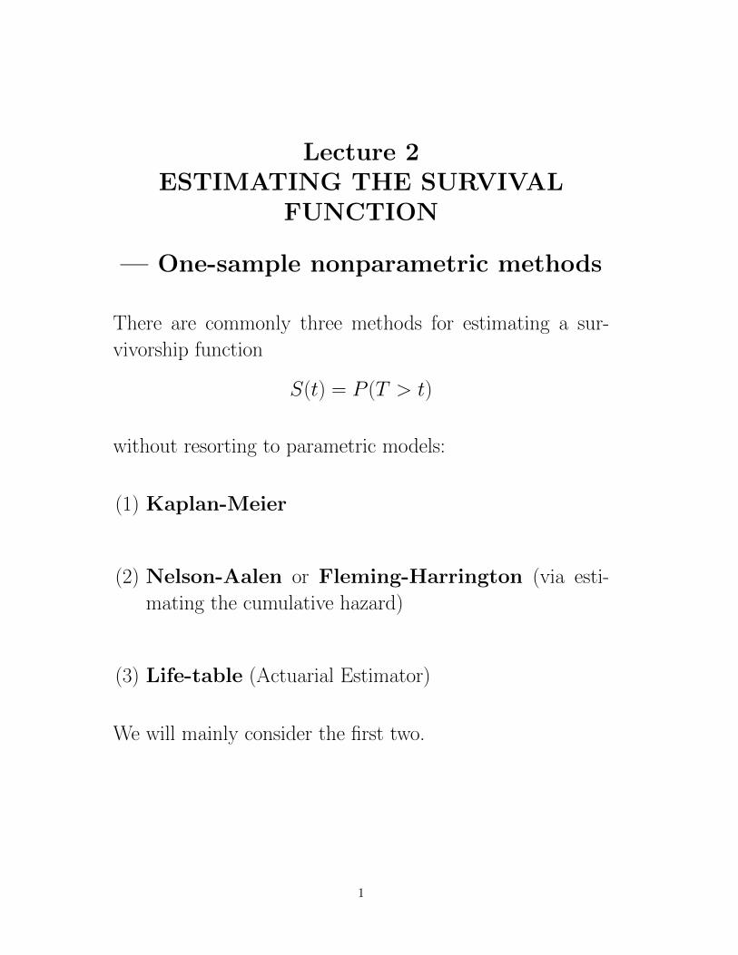
Extension to more than 2 events:

Suppose A1, A2...Ak are k different events. Then, the prob-

ability of all k events happening together can be written as

a product of conditional probabilities:

P (A1 ∩ A2... ∩ Ak) = P (Ak|Ak−1 ∩ ... ∩ A1)××P (Ak−1|Ak−2 ∩ ... ∩ A1)

...

×P (A2|A1)

×P (A1)

7

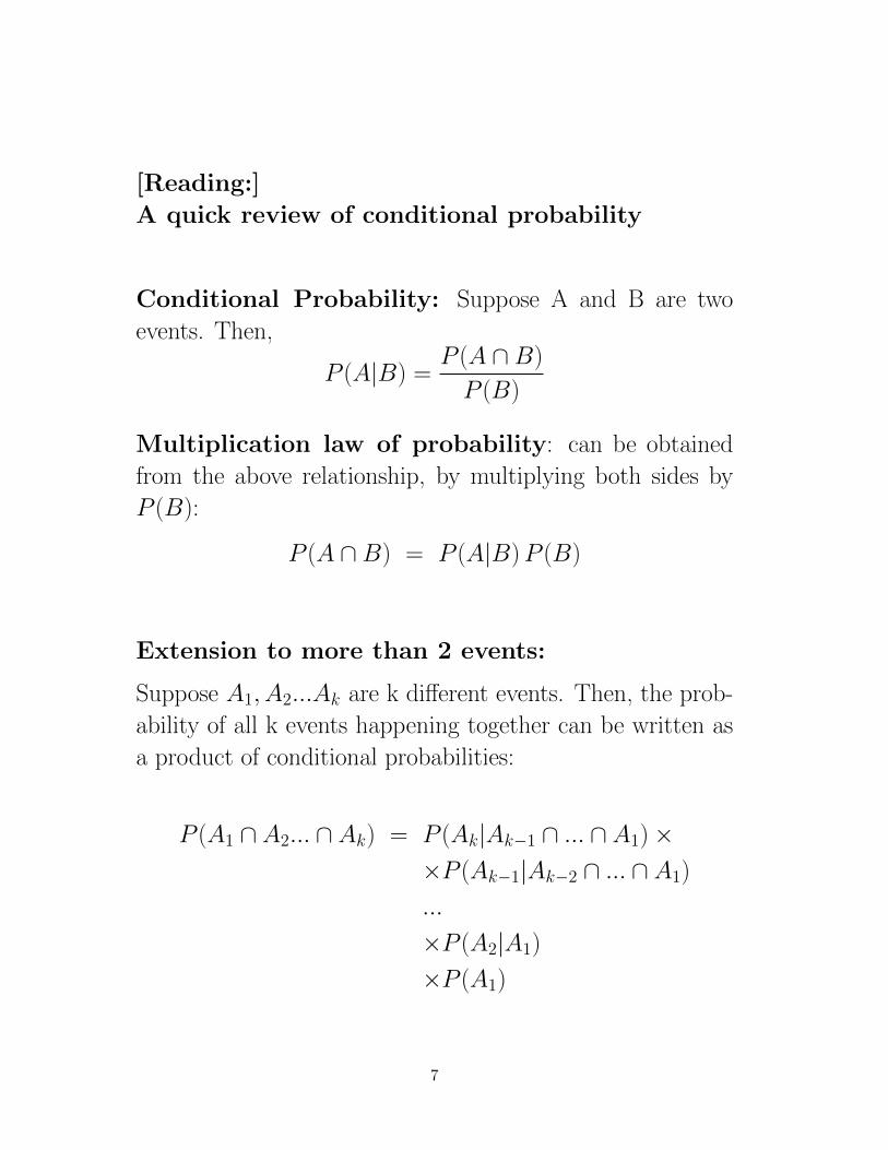
Now, let’s apply these ideas to estimate S(t):

– Intuition behind the Kaplan-Meier Estimator

Think of dividing the observed timespan of the study into a

series of fine intervals so that there is a separate interval for

each time of death or censoring:

D C C D D D

Using the law of conditional probability,

P (T > t) =∏j

P (survive j-th interval Ij | survived to start of Ij)

=∏j

λj

where the product is taken over all the intervals preceding

time t.

8

4 possibilities for each interval:

(1) No death or censoring - conditional probability of

surviving the interval is 1;

(2) Censoring - assume they survive to the end of the

interval (the intervals are very small), so that the condi-

tional probability of surviving the interval is 1;

(3) Death, but no censoring - conditional probability

of not surviving the interval is # deaths (d) divided by #

‘at risk’ (r) at the beginning of the interval. So the con-

ditional probability of surviving the interval is 1− d/r;

(4) Tied deaths and censoring - assume censorings last

to the end of the interval, so that conditional probability

of surviving the interval is still 1− d/r.

General Formula for jth interval:

It turns out we can write a general formula for the conditional

probability of surviving the j-th interval that holds for all 4

cases:

1− djrj

9

We could use the same approach by grouping the event times

into intervals (say, one interval for each month), and then

counting up the number of deaths (events) in each to esti-

mate the probability of surviving the interval (this is called

the lifetable estimate).

However, the assumption that those censored last until the

end of the interval wouldn’t be quite accurate, so we would

end up with a cruder approximation.

Here as the intervals get finer and finer, the approximations

made in estimating the probabilities of getting through each

interval become more and more accurate, at the end the

estimator converges to the true S(t) in probability (proof

not shown here).

This intuition explains why an alternative name for the KM

is the product-limit estimator.

10

The Kaplan-Meier estimator of the survivorship

function (or survival probability) S(t) = P (T > t)

is:

S(t) =∏

j:τj≤trj−djrj

=∏

j:τj≤t

(1− dj

rj

)where

• τ1, ...τK is the set of K distinct uncensored failure times

observed in the sample

• dj is the number of failures at τj

• rj is the number of individuals “at risk” right before

the j-th failure time (everyone who died or censored

at or after that time).

Furthermore, let cj be the number of censored observations

between the j-th and (j+ 1)-st failure times. Any censoring

tied at τj are included in cj, but not censorings tied at τj+1.

Note: two useful formulas are:

(1) rj = rj−1 − dj−1 − cj−1

(2) rj =∑l≥j

(cl + dl)

11

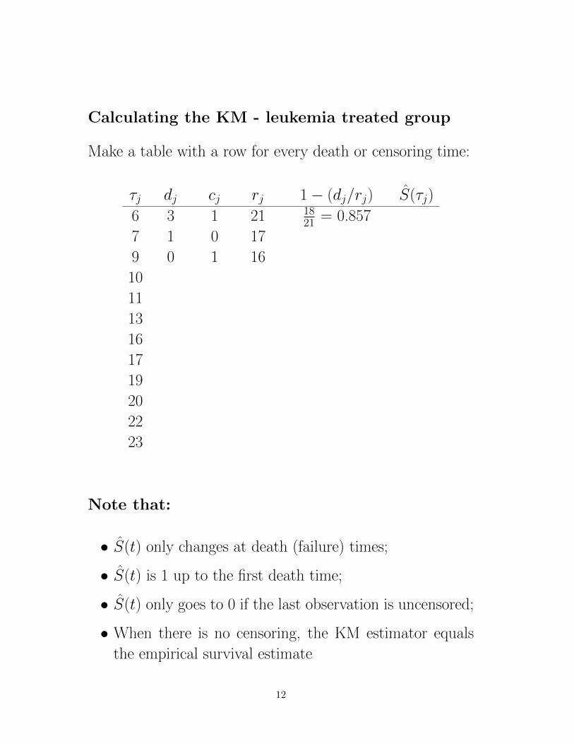
Calculating the KM - leukemia treated group

Make a table with a row for every death or censoring time:

τj dj cj rj 1− (dj/rj) S(τj)

6 3 1 21 1821 = 0.857

7 1 0 17

9 0 1 16

10

11

13

16

17

19

20

22

23

Note that:

• S(t) only changes at death (failure) times;

• S(t) is 1 up to the first death time;

• S(t) only goes to 0 if the last observation is uncensored;

• When there is no censoring, the KM estimator equals

the empirical survival estimate

12

Time

Sur

viva

l

0 5 10 15 20 25 30 35

0.0

0.2

0.4

0.6

0.8

1.0

Figure 2: KM plot for treated leukemia patients

Output from a software KM Estimator:

failure time: weeks

failure/censor: remiss

Beg. Net Survivor Std.

Time Total Fail Lost Function Error [95% Conf. Int.]

-------------------------------------------------------------------

6 21 3 1 0.8571 0.0764 0.6197 0.9516

7 17 1 0 0.8067 0.0869 0.5631 0.9228

9 16 0 1 0.8067 0.0869 0.5631 0.9228

10 15 1 1 0.7529 0.0963 0.5032 0.8894

11 13 0 1 0.7529 0.0963 0.5032 0.8894

13 12 1 0 0.6902 0.1068 0.4316 0.8491

16 11 1 0 0.6275 0.1141 0.3675 0.8049

13

17 10 0 1 0.6275 0.1141 0.3675 0.8049

19 9 0 1 0.6275 0.1141 0.3675 0.8049

20 8 0 1 0.6275 0.1141 0.3675 0.8049

22 7 1 0 0.5378 0.1282 0.2678 0.7468

23 6 1 0 0.4482 0.1346 0.1881 0.6801

25 5 0 1 0.4482 0.1346 0.1881 0.6801

32 4 0 2 0.4482 0.1346 0.1881 0.6801

34 2 0 1 0.4482 0.1346 0.1881 0.6801

35 1 0 1 0.4482 0.1346 0.1881 0.6801

(Note: the above is from Stata, but most software output

similar KM tables.)

14

[Reading:] Redistribution to the right algorithm

(Efron, 1967)

There is another way to compute the KM estimator.

In the absence of censoring, S(t) is just the proportion of

individuals with T > t. The idea behind Efron’s approach

is to spread the contributions of censored observations out

over all the possible times to their right.

Algorithm:

• Step (1): arrange the n observation times (failures or

censorings) in increasing order. If there are ties, put

censored after failures.

• Step (2): Assign weight (1/n) to each time.

• Step (3): Moving from left to right, each time you en-

counter a censored observation, distribute its mass to all

times to its right.

• Step (4): Calculate Sj by subtracting the final weight

for time j from Sj−1

15

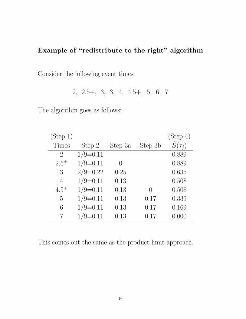
Example of “redistribute to the right” algorithm

Consider the following event times:

2, 2.5+, 3, 3, 4, 4.5+, 5, 6, 7

The algorithm goes as follows:

(Step 1) (Step 4)

Times Step 2 Step 3a Step 3b S(τj)

2 1/9=0.11 0.889

2.5+ 1/9=0.11 0 0.889

3 2/9=0.22 0.25 0.635

4 1/9=0.11 0.13 0.508

4.5+ 1/9=0.11 0.13 0 0.508

5 1/9=0.11 0.13 0.17 0.339

6 1/9=0.11 0.13 0.17 0.169

7 1/9=0.11 0.13 0.17 0.000

This comes out the same as the product-limit approach.

16

Properties of the KM estimator

When there is no censoring, KM estimator is the

same as the empirical estimator:

S(t) =# deaths after time t

n

where n is the number of individuals in the study.

As said before

S(t)asymp.∼ N (S(t), S(t)[1− S(t)]/n)

How does censoring affect this?

• S(t) is still consistent for the true S(t);

• S(t) is still asymptotically normal;

• The variance is more complicated.

The proofs can be done using the usual method (by writing

as sum of i.i.d. terms plus op(1)) but it is laborious, or it

can be done using counting processes which was considered

more elegant, or by empirical processes method which is

very powerful for semiparametric inferences.

17

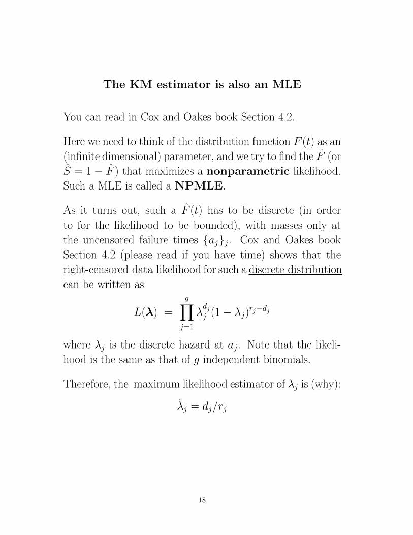
The KM estimator is also an MLE

You can read in Cox and Oakes book Section 4.2.

Here we need to think of the distribution function F (t) as an

(infinite dimensional) parameter, and we try to find the F (or

S = 1− F ) that maximizes a nonparametric likelihood.

Such a MLE is called a NPMLE.

As it turns out, such a F (t) has to be discrete (in order

to for the likelihood to be bounded), with masses only at

the uncensored failure times {aj}j. Cox and Oakes book

Section 4.2 (please read if you have time) shows that the

right-censored data likelihood for such a discrete distribution

can be written as

L(λ) =

g∏j=1

λdjj (1− λj)rj−dj

where λj is the discrete hazard at aj. Note that the likeli-

hood is the same as that of g independent binomials.

Therefore, the maximum likelihood estimator of λj is (why):

λj = dj/rj

18

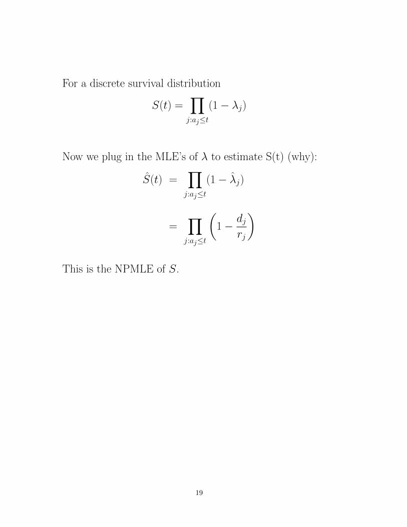
For a discrete survival distribution

S(t) =∏j:aj≤t

(1− λj)

Now we plug in the MLE’s of λ to estimate S(t) (why):

S(t) =∏j:aj≤t

(1− λj)

=∏j:aj≤t

(1− dj

rj

)

This is the NPMLE of S.

19

Greenwood’s formula for variance

Note that the KM estimator is

S(t) =∏j:τj≤t

(1− λj)

where λj = dj/rj.

Since the λj’s are just binomial proportions given rj’s, then

Var(λj) ≈λj(1− λj)

rj

Also, the λj’s are asymptotically independent.

Since S(t) is a function of the λj’s, we can estimate its vari-

ance using the Delta method.

Delta method: If Yn is (asymptotically) normal

with mean µ and variance σ2, g is differentiable and

g′(µ) 6= 0, then g(Yn) is approximately normally

distributed with mean g(µ) and variance [g′(µ)]2σ2.

20

Greenwood’s formula (continued)

Instead of dealing with S(t) directly, we will look at its log

(why?):

log[S(t)] =∑j:τj≤t

log(1− λj)

Thus, by approximate independence of the λj’s,

Var(log[S(t)]) =∑j:τj≤t

Var[log(1− λj)]

=∑j:τj≤t

(1

1− λj

)2

Var(λj)

=∑j:τj≤t

(1

1− λj

)2λj(1− λj)

rj

=∑j:τj≤t

λj

(1− λj)rj

=∑j:τj≤t

dj(rj − dj)rj

Now, S(t) = exp[log[S(t)]]. Using Delta method once again,

Var(S(t)) = [S(t)]2 · Var[log[S(t)]

]

21

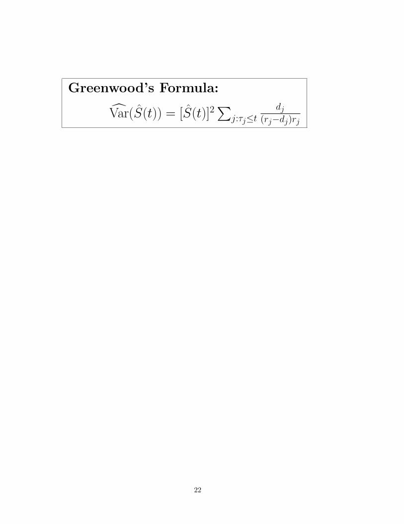
Greenwood’s Formula:

Var(S(t)) = [S(t)]2∑

j:τj≤tdj

(rj−dj)rj

22

Confidence intervals

For a 95% confidence interval, we could use

S(t)± z1−α/2 se[S(t)]

where se[S(t)] is calculated using Greenwood’s formula. Here

t is fixed, and this is refered to as pointwise confidence in-

terval.

Problem: This approach can yield values > 1 or < 0.

Better approach: Get a 95% confidence interval for

L(t) = log(− log(S(t)))

Since this quantity is unrestricted, the confidence interval

will be in the right range when we transform back:

S(t) = exp(− exp(L(t)).

[ To see why this works:

0 ≤ S(t) ≤ 1

−∞ ≤ log[S(t)] ≤ 0

0 ≤ − log[S(t)] ≤ ∞

−∞ ≤ log[− log[S(t)]

]≤ ∞

]

23

Log-log Approach for Confidence Intervals:

(1) Define L(t) = log(− log(S(t)))

(2) Form a 95% confidence interval for L(t) based on L(t),

yielding [L(t)− A, L(t) + A]

(3) Since S(t) = exp(− exp(L(t)), the confidence bounds

for the 95% CI of S(t) are:[exp{−eL(t)+A}, exp{−eL(t)−A}

](note that the upper and lower bounds switch)

(4) Substituting L(t) = log(− log(S(t))) back into the above

bounds, we get confidence bounds of([S(t)]e

A, [S(t)]e

−A)

24

What is A?

• A is 1.96 · se(L(t))

• To calculate this, we need to calculate

Var(L(t)) = Var[log(− log(S(t)))

]• From our previous calculations, we know

Var(log[S(t)]) =∑j:τj≤t

dj(rj − dj)rj

• Applying the delta method again, we get:

Var(L(t)) = Var(log(− log[S(t)]))

=1

[log S(t)]2

∑j:τj≤t

dj(rj − dj)rj

• We take the square root of the above to get se(L(t)),

25

Time

Sur

viva

l

0 5 10 15 20 25 30 35

0.0

0.2

0.4

0.6

0.8

1.0

Figure 3: KM Survival Estimate and Confidence intervals (type ‘log-log’)

• Different software might use different approaches to cal-

culate the CI.

Software for Kaplan-Meier Curves

• Stata - stset and sts commands

• SAS - proc lifetest

• R - survfit() in ‘survival’ package

26

R allows different types of CI (some are truncated to bebetween 0 and 1):

95 percent confidence interval is of type "log"

time n.risk n.event survival std.dev lower 95% CI upper 95% CI

6 21 3 0.8571429 0.07636035 0.7198171 1.0000000

7 17 1 0.8067227 0.08693529 0.6531242 0.9964437

10 15 1 0.7529412 0.09634965 0.5859190 0.9675748

13 12 1 0.6901961 0.10681471 0.5096131 0.9347692

16 11 1 0.6274510 0.11405387 0.4393939 0.8959949

22 7 1 0.5378151 0.12823375 0.3370366 0.8582008

23 6 1 0.4481793 0.13459146 0.2487882 0.8073720

95 percent confidence interval is of type "log-log"

time n.risk n.event survival std.dev lower 95% CI upper 95% CI

6 21 3 0.8571429 0.07636035 0.6197180 0.9515517

7 17 1 0.8067227 0.08693529 0.5631466 0.9228090

10 15 1 0.7529412 0.09634965 0.5031995 0.8893618

13 12 1 0.6901961 0.10681471 0.4316102 0.8490660

16 11 1 0.6274510 0.11405387 0.3675109 0.8049122

22 7 1 0.5378151 0.12823375 0.2677789 0.7467907

23 6 1 0.4481793 0.13459146 0.1880520 0.6801426

95 percent confidence interval is of type "plain"

time n.risk n.event survival std.dev lower 95% CI upper 95% CI

6 21 3 0.8571429 0.07636035 0.7074793 1.0000000

7 17 1 0.8067227 0.08693529 0.6363327 0.9771127

10 15 1 0.7529412 0.09634965 0.5640993 0.9417830

13 12 1 0.6901961 0.10681471 0.4808431 0.8995491

16 11 1 0.6274510 0.11405387 0.4039095 0.8509924

22 7 1 0.5378151 0.12823375 0.2864816 0.7891487

23 6 1 0.4481793 0.13459146 0.1843849 0.7119737

27

Mean, Median, Quantiles based on the KM

• Mean is not well estimated with censored data, since we

often don’t observe the right tail.

•Median - by definition, this is the time, τ , such that

S(τ ) = 0.5. In practice, it is often defined as the small-

est time such that S(τ ) ≤ 0.5. The median is more

appropriate for censored survival data than the mean.

For the treated leukemia patients, we find:

S(22) = 0.5378

S(23) = 0.4482

The median is thus 23.

• Lower quartile (25th percentile):

the smallest time (LQ) such that S(LQ) ≤ 0.75

• Upper quartile (75th percentile):

the smallest time (UQ) such that S(UQ) ≤ 0.25

28

Left truncated KM estimate

Suppose that there is left truncation, so the observed data

is (Qi, Xi, δi), i = 1, ..., n.

Now the ‘risk set’ at any time t consists of subjects who have

entered the study, and have not failed or been censored by

that time, i.e. {i : Qi < t ≤ Xi}.

So rj =∑n

i=1 I(Qi < τj ≤ Xi).

We still have

S(t) =∏j:τj≤t

(1− dj

rj

)where τ1, ...τK is the set of K distinct uncensored failure

times observed in the sample, dj is the number of failures at

τj, and rj is the number of individuals “at risk” right before

the j-th failure time (everyone who had entered and

who died or censored at or after that time).

When minni=1Qi = t0 > 0, then the KM estimates P (T >

t|T > t0).

29

• The left truncated KM is still an NPMLE (Wang, 1991).

• The Greenwood’s formula for variance still applies.

• In R (and most other softwares) it is handled by some-

thing like ‘Surv(time=Q, time2=X , event=δ)’.

• Read [required] Tsai, Jewell and Wang (1987).

30

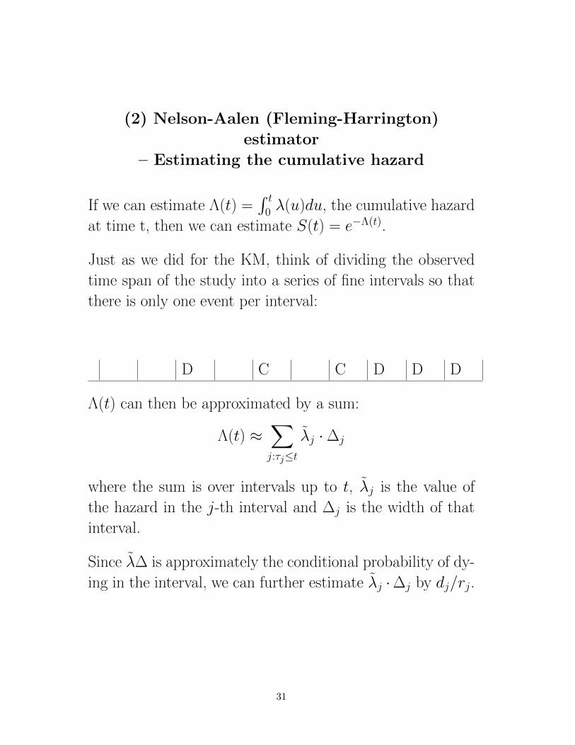
(2) Nelson-Aalen (Fleming-Harrington)

estimator

– Estimating the cumulative hazard

If we can estimate Λ(t) =∫ t

0 λ(u)du, the cumulative hazard

at time t, then we can estimate S(t) = e−Λ(t).

Just as we did for the KM, think of dividing the observed

time span of the study into a series of fine intervals so that

there is only one event per interval:

D C C D D D

Λ(t) can then be approximated by a sum:

Λ(t) ≈∑j:τj≤t

λj ·∆j

where the sum is over intervals up to t, λj is the value of

the hazard in the j-th interval and ∆j is the width of that

interval.

Since λ∆ is approximately the conditional probability of dy-

ing in the interval, we can further estimate λj ·∆j by dj/rj.

31

This gives the Nelson-Aalen estimator:

ΛNA(t) =∑j:τj≤t

dj/rj.

It follows that Λ(t), like the KM, changes only at the ob-

served death (event) times.

Example:

D C C D D D

rj n n n n-1 n-1 n-2 n-2 n-3 n-4

dj 0 0 1 0 0 0 0 1 1

cj 0 0 0 0 1 0 1 0 0

λ(tj)∆ 0 0 1/n 0 0 0 0 1n−3

1n−4

Λ(tj) 0 0 1/n 1/n 1/n 1/n 1/n

Once we have ΛNA(t), we can obtain the Fleming-Harrington

estimator of S(t):

SFH(t) = exp(−ΛNA(t)).

32

In general, the FH estimator of the survival function should

be close to the Kaplan-Meier estimator, SKM(t).

We can compare the Fleming-Harrington survival estimate

to the KM estimate using a subgroup of the nursing home

data:

skm sfh

1. .91666667 .9200444

2. .83333333 .8400932

3. .75 .7601478

4. .66666667 .6802101

5. .58333333 .6002833

6. .5 .5203723

7. .41666667 .4404857

8. .33333333 .3606392

9. .25 .2808661

10. .16666667 .2012493

11. .08333333 .1220639

12. 0 .0449048

In this example, it looks like the Fleming-Harrington estima-

tor is slightly higher than the KM at every time point, but

with larger datasets the two will typically be much closer.

Question: do you think that the two estimators are asymp-

totically equivalent?

33

Note: We can also go the other way: we can take the

Kaplan-Meier estimate of S(t), and use it to calculate an

alternative estimate of the cumulative hazard function:

ΛKM(t) = − log SKM(t)

34

[Reading:]

(3) The Lifetable or Actuarial Estimator

• one of the oldest techniques around

• used by actuaries, demographers, etc.

• applies when the data are grouped

Our goal is still to estimate the survival function, hazard,

and density function, but this is sometimes complicated by

the fact that we don’t know exactly when during a time

interval an event occurs.

35

There are several types of lifetable methods according to the

data sources:

Population Life Tables

• cohort life table - describes the mortality experience

from birth to death for a particular cohort of people born

at about the same time. People at risk at the start of the

interval are those who survived the previous interval.

• current life table - constructed from (1) census infor-

mation on the number of individuals alive at each age,

for a given year and (2) vital statistics on the number

of deaths or failures in a given year, by age. This type

of lifetable is often reported in terms of a hypothetical

cohort of 100,000 people.

Generally, censoring is not an issue for Population Life Ta-

bles.

Clinical Life tables - applies to grouped survival data

from studies in patients with specific diseases. Because pa-

tients can enter the study at different times, or be lost to

follow-up, censoring must be allowed.

36

Notation

• the j-th time interval is [tj−1, tj)

• cj - the number of censorings in the j-th interval

• dj - the number of failures in the j-th interval

• rj is the number entering the interval

Example: 2418 Males with Angina Pectoris (chest pain,

from book by Lee, p.91)

Year after

Diagnosis j dj cj rj r′j = rj − cj/2

[0, 1) 1 456 0 2418 2418.0

[1, 2) 2 226 39 1962 1942.5 (1962 - 392 )

[2, 3) 3 152 22 1697 1686.0

[3, 4) 4 171 23 1523 1511.5

[4, 5) 5 135 24 1329 1317.0

[5, 6) 6 125 107 1170 1116.5

[6, 7) 7 83 133 938 871.5

etc..

37

Estimating the survivorship function

If we apply the KM formula directly to the numbers in the

table on the previous page, estimating S(t) as

S(t) =∏j:τj<t

(1− dj

rj

),

this approach is unsatisfactory for grouped data because

it treats the problem as though it were in discrete time,

with events happening only at 1 yr, 2 yr, etc. In fact, we

should try to calculate the conditional probability of dying

within the interval, given survival to the beginning of it.

What should we do with the censored subjects?

Let r′j denote the ‘effective’ number of subjects at risk. If we

assume that censorings occur:

• at the beginning of each interval: r′j = rj − cj• at the end of each interval: r′j = rj

• on average halfway through the interval:

r′j = rj − cj/2

The last assumption yields the Actuarial Estimator. It is

appropriate if censorings occur uniformly throughout the in-

terval.

38

Constructing the lifetable

First, some additional notation for the j-th interval, [tj−1, tj):

•Midpoint (tmj) - useful for plotting the density and

the hazard function

•Width (bj = tj−tj−1) needed for calculating the hazard

in the j-th interval

Quantities estimated:

• Conditional probability of dying (event)

qj = dj/r′j

• Conditional probability of surviving

pj = 1− qj

• Cumulative probability of surviving at tj:

S(tj) =∏`≤j

p`

=∏`≤j

(1− d`

r′`

)

39

Other quantities estimated at the

midpoint of the j-th interval:

• Hazard in the j-th interval (why)

λ(tmj) =dj

bj(r′j − dj/2)

=qj

bj(1− qj/2)

• density at the midpoint of the j-th interval (why)

f (tmj) =S(tj−1)− S(tj)

bj

=S(tj−1) qj

bj

Note: Another way to get this is:

f (tmj) = λ(tmj)S(tmj)

= λ(tmj)[S(tj) + S(tj−1)]/2

40

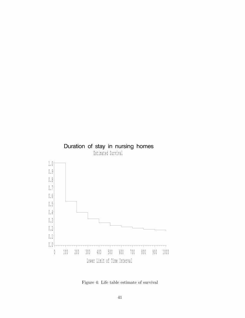
E s t i m a t e d S u r v i v a l

0 . 00 . 10 . 20 . 30 . 40 . 50 . 60 . 70 . 80 . 91 . 0

L o w e r L i m i t o f T i m e I n t e r v a l0 1 0 0 2 0 0 3 0 0 4 0 0 5 0 0 6 0 0 7 0 0 8 0 0 9 0 0 1 0 0 0

Figure 4: Life table estimate of survival

41

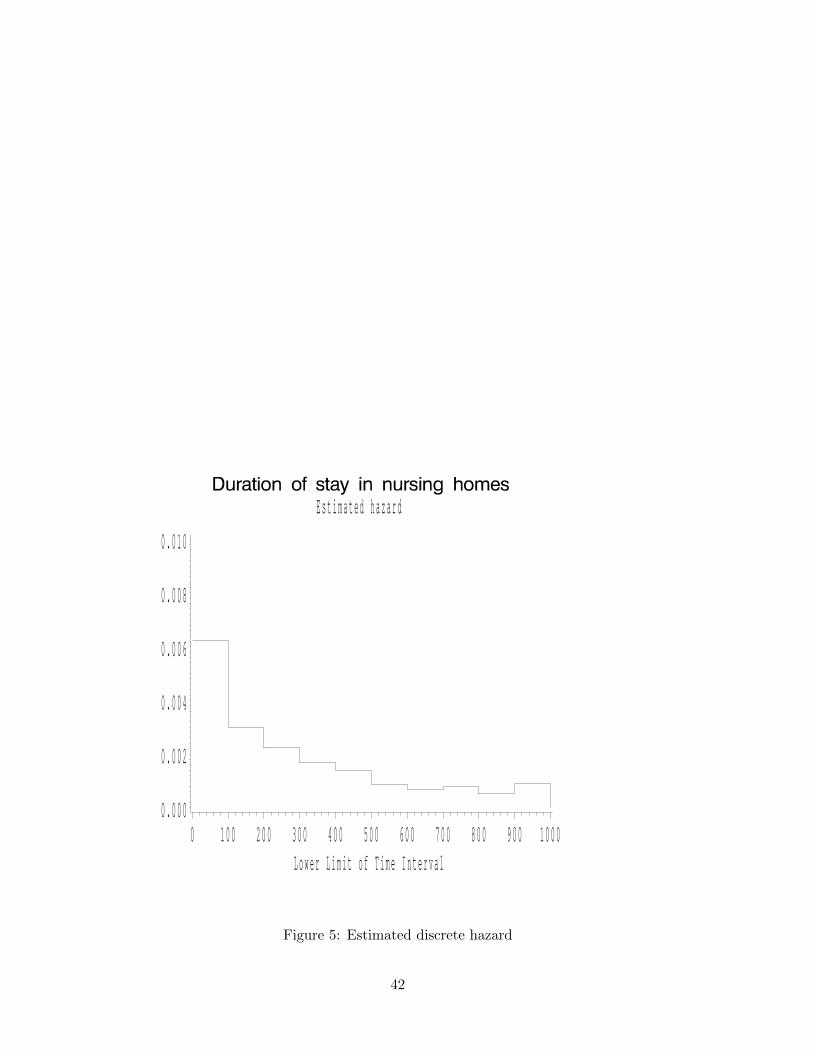
E s t i m a t e d h a z a r d

0 . 0 0 0

0 . 0 0 2

0 . 0 0 4

0 . 0 0 6

0 . 0 0 8

0 . 0 1 0

L o w e r L i m i t o f T i m e I n t e r v a l0 1 0 0 2 0 0 3 0 0 4 0 0 5 0 0 6 0 0 7 0 0 8 0 0 9 0 0 1 0 0 0

Figure 5: Estimated discrete hazard

42