Lecture 2 - 1 tjwc - 17-Jun-15ISE1/EE2 Computing - Matlab Matlab Lecture 2: More MATLAB Programming u MATLAB has five flow control constructs: if statements

Lecture 2 - 1tjwc - Apr 18, 2023 ISE1/EE2 Computing - Matlab

Matlab Lecture 2: More MATLAB Programming

MATLAB has five flow control constructs:

if statements

switch statements

for loops

while loops

break statements

if statement if A > B 'greater'elseif A < B 'less'elseif A == B 'equal'else error('Unexpected situation')end

>, < and == work withscalars, but NOT

matrices


Matrix Comparison - Beware!

16 2 3 13 5 11 10 8 9 7 6 12 4 14 15 1

16 2 3 13 5 11 10 8 9 7 6 12 4 14 15 1

16 5 9 4 2 11 7 14 3 10 6 1513 8 12 1

16 5 9 4 2 11 7 14 3 10 6 1513 8 12 1

A

B

» A=magic(4)

» B = A’

1 0 0 00 1 0 00 0 1 00 0 0 1

1 0 0 00 1 0 00 0 1 00 0 0 1

0 0 0 11 0 1 01 0 0 00 1 1 0

0 0 0 11 0 1 01 0 0 00 1 1 0

0 1 1 00 0 0 10 1 0 11 0 0 0

0 1 1 00 0 0 10 1 0 11 0 0 0

C=A>B

C=(A==B)

C=A<B

1 = true

0 = false


Built-in Logic functions for matrices

Several functions are helpful for reducing the results of matrix comparisons to scalar conditions for use with if, including isequal(A,B) returns ‘1’ if A and B are identical, else return ‘0’ isempty(A) returns ‘1’ if A is a null matrix, else return ‘0’ all(A) returns ‘1’ if all elements A is non-zero any(A) returns ‘1’ if any element A is non-zero

if isequal(A,B) 'equal'else 'not equal'end

if isequal(A,B) 'equal'else 'not equal'end


Control Flow - Switch & Case

Assume method exists as a string variable:

switch lower(method) case {'linear','bilinear'}

disp('Method is linear') case 'cubic’

disp('Method is cubic') case 'nearest’

disp('Method is nearest')

otherwisedisp('Unknown method.')

end

Assume method exists as a string variable:

switch lower(method) case {'linear','bilinear'}

disp('Method is linear') case 'cubic’

disp('Method is cubic') case 'nearest’

disp('Method is nearest')

otherwisedisp('Unknown method.')

end

Use otherwise tocatch all other cases


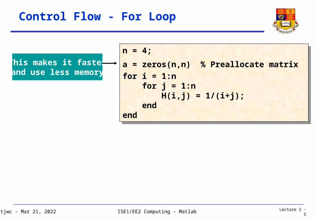
Control Flow - For Loop

n = 4;

a = zeros(n,n) % Preallocate matrix

for i = 1:n for j = 1:n H(i,j) = 1/(i+j); endend

n = 4;

a = zeros(n,n) % Preallocate matrix

for i = 1:n for j = 1:n H(i,j) = 1/(i+j); endend

This makes it fasterand use less memory


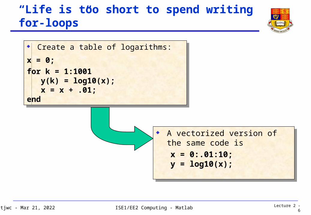
“Life is too short to spend writing for-loops”

Create a table of logarithms:

x = 0;

for k = 1:1001 y(k) = log10(x); x = x + .01;end

Create a table of logarithms:

x = 0;

for k = 1:1001 y(k) = log10(x); x = x + .01;end

A vectorized version of the same code is

x = 0:.01:10;y = log10(x);

A vectorized version of the same code is

x = 0:.01:10;y = log10(x);


Control Flow - While Loop

eps = 0.0001a = 0; fa = -Inf;b = 3; fb = Inf;while b-a > eps*b x = (a+b)/2; fx = x^3-2*x-5; if sign(fx) == sign(fa) a = x; fa = fx; else b = x; fb = fx; endendx

eps = 0.0001a = 0; fa = -Inf;b = 3; fb = Inf;while b-a > eps*b x = (a+b)/2; fx = x^3-2*x-5; if sign(fx) == sign(fa) a = x; fa = fx; else b = x; fb = fx; endendx

Find root of the polynomial x3 - 2x - 5 ..

… using iterative bisection method


Control Flow - break

The break statement lets you exit early from a for or while loop.

In nested loops, break exits from the innermost loop only.

Why is this version of the bisection programme better?

a = 0; fa = -Inf;

b = 3; fb = Inf;while b-a > eps*b x = (a+b)/2; fx = x^3-2*x-5; if fx == 0 break elseif sign(fx) == sign(fa) a = x; fa = fx; else b = x; fb = fx; endendx

a = 0; fa = -Inf;

b = 3; fb = Inf;while b-a > eps*b x = (a+b)/2; fx = x^3-2*x-5; if fx == 0 break elseif sign(fx) == sign(fa) a = x; fa = fx; else b = x; fb = fx; endendx


Matrix versus Array Operations

16 3 2 13 5 10 11 8 9 6 7 12 4 15 14 1

16 3 2 13 5 10 11 8 9 6 7 12 4 15 14 1

A

341 285 261 269261 301 309 285285 309 301 261269 261 285 341

341 285 261 269261 301 309 285285 309 301 261269 261 285 341

256 9 4 16925 100 121 6481 36 49 14416 225 196 1

256 9 4 16925 100 121 6481 36 49 14416 225 196 1

A * A

A .* A

Inner product matrix multiply

Element-by-element array multiply


Matrix Operators


Array Operators


M-files: Scripts and Functions

There are two kinds of M-files:

Scripts, which do not accept input arguments or return output arguments. They operate on data in the workspace.

Functions, which can accept input arguments and return output arguments. Internal variables are local to the function.

% Investigate the rank of magic squares

r = zeros(1,32);for n = 3:32

r(n) = rank(magic(n));endrbar(r)

% Investigate the rank of magic squares

r = zeros(1,32);for n = 3:32

r(n) = rank(magic(n));endrbar(r)

Script magic_rank.m


Functions

function r = myfunct (x)% Calculate the function:% r = x^3 - 2*x - 5% x can be a vector

r = x.^3 - x.*2 -5;

function r = myfunct (x)% Calculate the function:% r = x^3 - 2*x - 5% x can be a vector

r = x.^3 - x.*2 -5;

Define function name and argumentsReturn variable

% on column 1 is a comment

» X = 0:0.05:3;» y = myfunct (x);» plot(x,y)

» X = 0:0.05:3;» y = myfunct (x);» plot(x,y)

function myfunct.m

This is how plot on p.2-7 was obtained


Scopes of variables

All variables used inside a function are local to that function Parameters are passed in and out of the function explicitly as

defined by the first line of the function You can use the keyword global to make a variable visible

everywhere As a good programming practice, only use global variables

when it is absolutely required


MATLAB Programming Style Guide (1)

This Style Guideline is originally prepared by Mike Cook

The first line of code in script m-files should be indicate the name of

the file.

The first line of function m-files has a mandatory structure. The first line of a function is a declaration line. It has the word function in it to identifies the file as a function, rather than a generic m-file. For example, for a function named abs_error.m, the the first line would be:

function [X,Y] = abs_error(A,B)

A block of comments should be placed at the top of the regular m-

files, and just after the function definition in function m-files. This is

the header comment block. The formats are different for m-files and

functions.


Style Guide (2)

Variables should have meaningful names. This will make your code easier to read, and will reduce the number of comments you will need. However here are some pitfalls about choosing variable names:

Meaningful variable names are good, but when the variable name gets to 15 characters or more, it tends to obscure rather than improve code.

The maximum length of a variable name is 19 characters and all variables must start with a character (not number).

Be careful of naming a variable that will conflict with matlab's built-in functions, or reserved names: if, while, end, pi, sin, cos, etc.

Avoid names that differ only in case, look similar, or differ only slightly from each other.

Make good use of white space, both horizontally and vertically, it will improve the readability of your program greatly.


Style Guide (3)

Comments describing tricky parts of the code, assumptions, or design decisions should be placed above the part of the code you are attempting to document.

Do not add comment statements to explain things that are obvious.

Try to avoid big blocks of comments except in the detailed description of the m-file in the header block.

Indenting. Lines of code and comments inside branching (if block) or repeating (for and while loop) logic structures will be indented 3 spaces. NOTE: don't use tabs, use spaces. For example:

for i=1:n disp('in loop') if data(i) < x disp('less than x') else disp('greater than or equal to x') end count = count + 1; end


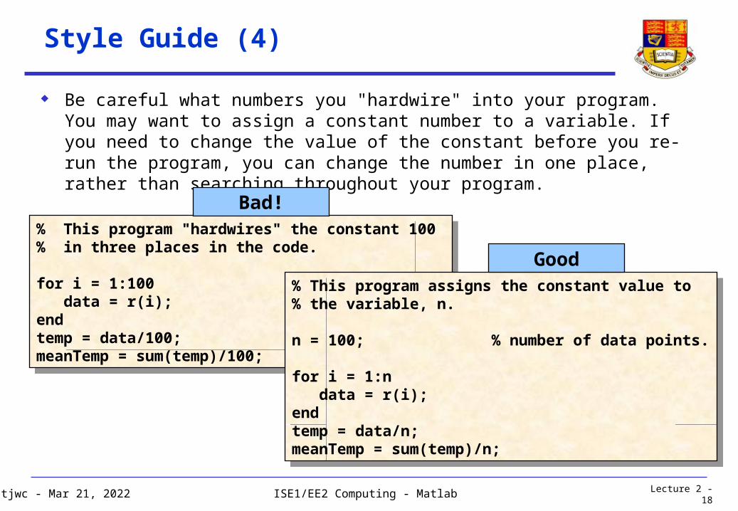
Style Guide (4)

Be careful what numbers you "hardwire" into your program. You may want to assign a constant number to a variable. If you need to change the value of the constant before you re-run the program, you can change the number in one place, rather than searching throughout your program.

% This program "hardwires" the constant 100 % in three places in the code.

for i = 1:100 data = r(i);endtemp = data/100;meanTemp = sum(temp)/100;

% This program "hardwires" the constant 100 % in three places in the code.

for i = 1:100 data = r(i);endtemp = data/100;meanTemp = sum(temp)/100;

% This program assigns the constant value to % the variable, n.

n = 100; % number of data points.

for i = 1:n data = r(i);endtemp = data/n;meanTemp = sum(temp)/n;

% This program assigns the constant value to % the variable, n.

n = 100; % number of data points.

for i = 1:n data = r(i);endtemp = data/n;meanTemp = sum(temp)/n;

Bad!

Good


Style Guide (5)

No more than one executable statement per line in your regular or function m-files.

No line of code should exceed 80 characters. (There may be a few times when this is not possible, but they are rare).

The comment lines of the function m-file are the printed to the screen when help is requested on that function.

function bias = bias_error(X,Y)% Purpose: Calculate the bias between input arrays X and Y% Input: X, Y, must be the same length% Output: bias = bias of X and Y % % filename: bias_error.m% Mary Jordan, 3/10/96%bias = sum(X-Y)/length(X);

function bias = bias_error(X,Y)% Purpose: Calculate the bias between input arrays X and Y% Input: X, Y, must be the same length% Output: bias = bias of X and Y % % filename: bias_error.m% Mary Jordan, 3/10/96%bias = sum(X-Y)/length(X);


Style Guide (6) - Another good example

function [out1,out2] = humps(x)%% Y = HUMPS(X) is a function with strong maxima near x = .3 % and x = .9. %% [X,Y] = HUMPS(X) also returns X. With no input arguments,% HUMPS uses X = 0:.05:1.%% Copyright (c) 1984-97 by The MathWorks, Inc.% $Revision: 5.3 $ $Date: 1997/04/08 05:34:37 $

if nargin==0, x = 0:.05:1; end

y = 1 ./ ((x-.3).^2 + .01) + 1 ./ ((x-.9).^2 + .04) - 6;

if nargout==2, out1 = x; out2 = y; else out1 = y;end

function [out1,out2] = humps(x)%% Y = HUMPS(X) is a function with strong maxima near x = .3 % and x = .9. %% [X,Y] = HUMPS(X) also returns X. With no input arguments,% HUMPS uses X = 0:.05:1.%% Copyright (c) 1984-97 by The MathWorks, Inc.% $Revision: 5.3 $ $Date: 1997/04/08 05:34:37 $

if nargin==0, x = 0:.05:1; end

y = 1 ./ ((x-.3).^2 + .01) + 1 ./ ((x-.9).^2 + .04) - 6;

if nargout==2, out1 = x; out2 = y; else out1 = y;end


Function of functions - fplot

% Plot function humps(x) with FPLOT

fplot('humps',[0,2])

FPLOT(FUN,LIMS) plots the function specified by the string FUN between the x-axis limits specified by LIMS = [XMIN XMAX]


Find Zero

% Find the zero of humps(x) with FZERO z = fzero('humps',1); fplot('humps',[0,2]); hold on; plot(z,0,'r*'); hold off

FZERO(F,X) tries to find a zero of F.FZERO looks for an interval containing a sign change for F and containing X.


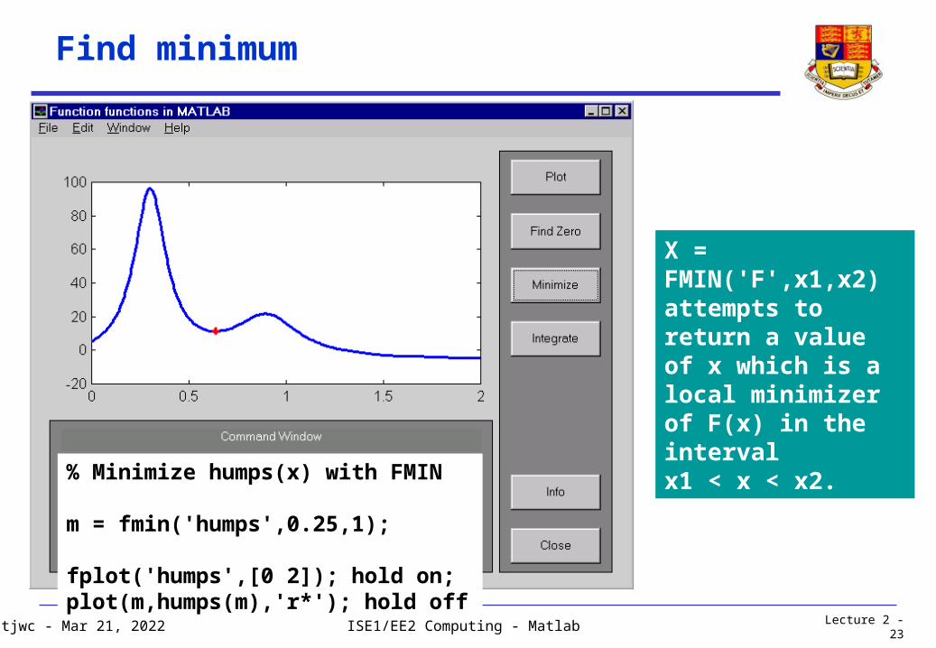
Find minimum

% Minimize humps(x) with FMIN m = fmin('humps',0.25,1); fplot('humps',[0 2]); hold on; plot(m,humps(m),'r*'); hold off

X = FMIN('F',x1,x2) attempts to return a value of x which is a local minimizer of F(x) in the interval x1 < x < x2.


Integration of Curve

% Compute integral with QUAD q = quad('humps',0.5,1); fplot('humps',[0,2]); title(['Area = ',num2str(q)]);

Q = QUAD('F',A,B) approximates the integral of F(X) from A to B to within a relative error of 1e-3 using an adaptive recursive Simpson's rule.

Documents

Lecture 2 - 1 tjwc - 17-Jun-15ISE1/EE2 Computing - Matlab Matlab Lecture 2: More MATLAB Programming u MATLAB has five flow control constructs: if statements