Embed Size (px)
Citation preview
Lecture 1(c) Lecture 1(c) Marginal Analysis Marginal Analysis and Optimizationand Optimization

Why is it important to understand Why is it important to understand the mathematics of optimization in the mathematics of optimization in
order to understand order to understand microeconomics?microeconomics?
The “economic way of thinking” The “economic way of thinking” assumes that individuals behave as if assumes that individuals behave as if they are “rational”. they are “rational”.
Question for the class: What does it Question for the class: What does it mean to say that behavior is mean to say that behavior is “rational”?“rational”?
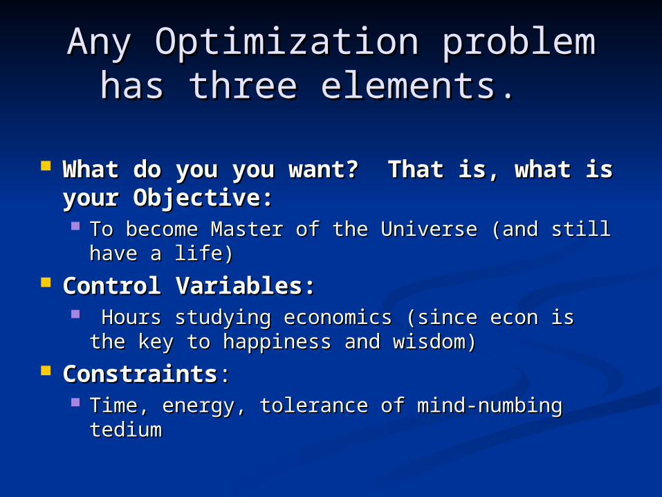
Any Optimization problem has Any Optimization problem has three elements. three elements.
What do you you want? That is, what is What do you you want? That is, what is your Objective:your Objective: To become Master of the Universe (and still have To become Master of the Universe (and still have
a life)a life) Control Variables: Control Variables:
Hours studying economics (since econ is the Hours studying economics (since econ is the key to happiness and wisdom)key to happiness and wisdom)
ConstraintsConstraints: : Time, energy, tolerance of mind-numbing tediumTime, energy, tolerance of mind-numbing tedium

The magic word: The magic word: “marginal”“marginal”
MARGINALMARGINAL ____ : The change in ____ ____ : The change in ____ when something else changes.when something else changes.
Approximate Formula: The marginal Approximate Formula: The marginal contribution of x to y=(change in contribution of x to y=(change in y)/(change in x)y)/(change in x)
Exact Formally (calculus): If y=f(x), Exact Formally (calculus): If y=f(x), the marginal contribution of x to y is the marginal contribution of x to y is dy/dx.dy/dx.
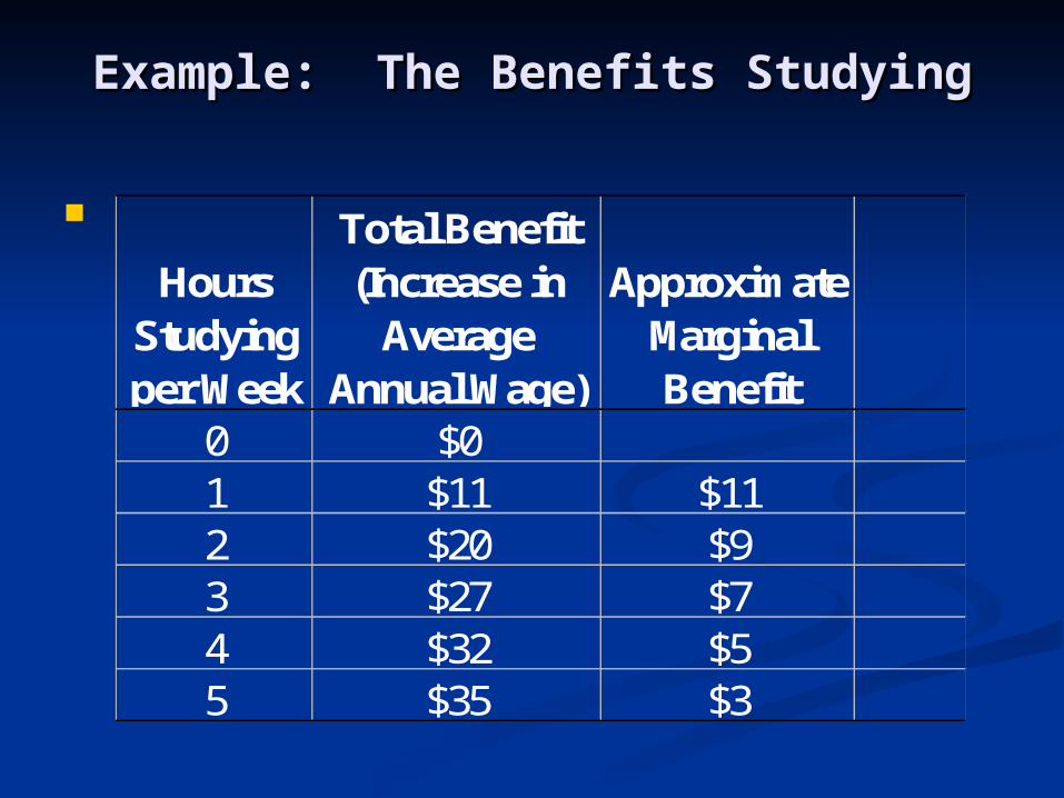
Example: The Benefits StudyingExample: The Benefits Studying
Hours Studying per Week
Total Benefit (Increase in
Average Annual Wage)
Approximate Marginal Benefit
0 $01 $11 $112 $20 $93 $27 $74 $32 $55 $35 $3

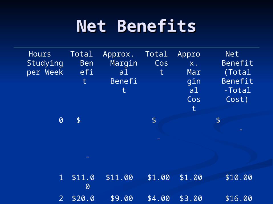
Benefits and CostsBenefits and Costs
Hours Studying per Week
Total Benefit (Increase
in Average Annual Wage)
Approx. Marginal Benefit
Total Cost Approx. Marginal
Cost
0 $ - 0
1 $11.00 $11.00 1 $1.00
2 $20.00 $9.00 4 $3.00
3 $27.00 $7.00 9 $5.00
4 $32.00 $5.00 16 $7.00
5 $35.00 $3.00 25 $9.00
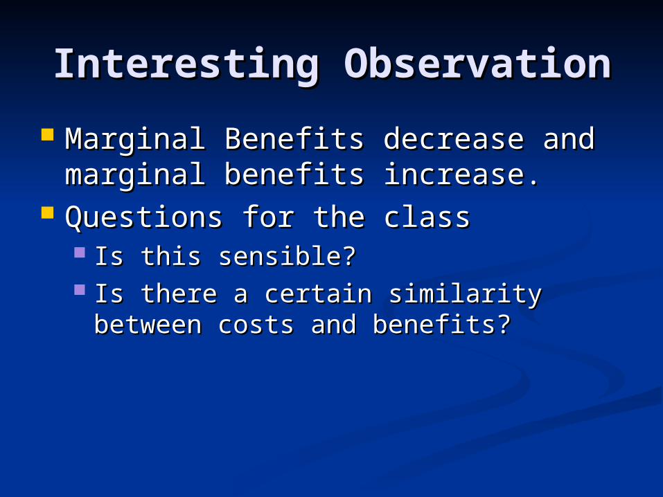
Interesting ObservationInteresting Observation
Marginal Benefits decrease and Marginal Benefits decrease and marginal benefits increase.marginal benefits increase.
Questions for the classQuestions for the class Is this sensible?Is this sensible? Is there a certain similarity between Is there a certain similarity between
costs and benefits?costs and benefits?
Net BenefitsNet Benefits
Hours Studying per Week
Total Benefit
Approx. Marginal Benefit
Total Cost
Approx. Marginal Cost
Net Benefit (Total
Benefit -Total Cost)
0 $ -
$ - $ -
1 $11.00 $11.00 $1.00 $1.00 $10.00
2 $20.00 $9.00 $4.00 $3.00 $16.00
3 $27.00 $7.00 $9.00 $5.00 $18.00
4 $32.00 $5.00 $16.00 $7.00 $16.00
5 $35.00 $3.00 $25.00 $9.00 $10.00

Net BenefitsNet BenefitsHours Studying per Week
Total Benefit
Approx. Marginal Benefit
Total Cost Approx. Marginal
Cost
Net Benefit (Total Benefit -Total
Cost)
0 $ -
$ - $ -
1 $11.00 $11.00 $1.00 $1.00 $10.00
2 $20.00 $9.00 $4.00 $3.00 $16.00
3 $27.00 $7.00 $9.00 $5.00 $18.00
4 $32.00 $5.00 $16.00 $7.00 $16.00
5 $35.00 $3.00 $25.00 $9.00 $10.00
3 hours is the best

Think About Optimization Think About Optimization as a Sequence of Stepsas a Sequence of Steps
Hours Studying per Week
Total Benefit
Approx. Marginal Benefit
Total Cost Approx. Marginal
Cost
Net Benefit (Total Benefit -Total
Cost)
0 $ -
$ - $ -
1 $11.00 $11.00 $1.00 $1.00 $10.00
2 $20.00 $9.00 $4.00 $3.00 $16.00
3 $27.00 $7.00 $9.00 $5.00 $18.00
4 $32.00 $5.00 $16.00 $7.00 $16.00
5 $35.00 $3.00 $25.00 $9.00 $10.00
If Here, Do More
If Here, Do Less

Common Sense ConclusionCommon Sense Conclusion
If marginal benefits are greater than If marginal benefits are greater than marginal costs, then do more.marginal costs, then do more.
If marginal benefits are less than If marginal benefits are less than marginal costs, then do less.marginal costs, then do less.
To optimize, find the level of activity To optimize, find the level of activity where marginal benefits with where marginal benefits with marginal costsmarginal costs

Applying the Principle to Applying the Principle to EquibaseEquibase
Our spreadsheets let us work with any Our spreadsheets let us work with any number of different assumptions about number of different assumptions about demand and costs, and so let’s assume demand and costs, and so let’s assume that Equibase merged with the tracksthat Equibase merged with the tracks
Objective: max profitsObjective: max profits Constraints are defined by the market Constraints are defined by the market
demand and the costs. Let’s assumedemand and the costs. Let’s assume Q=500(5-P)Q=500(5-P) Variable Production cost = $.5/unitVariable Production cost = $.5/unit Fixed production cost = $500Fixed production cost = $500
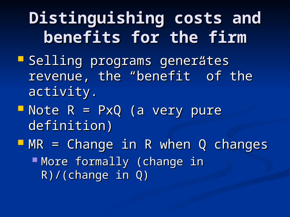
Distinguishing costs and Distinguishing costs and benefits for the firmbenefits for the firm
Selling programs generates revenue, Selling programs generates revenue, the “benefit” of the activity.the “benefit” of the activity.
Note R = PxQ (a very pure Note R = PxQ (a very pure definition)definition)
MR = Change in R when Q changesMR = Change in R when Q changes More formally (change in R)/(change in More formally (change in R)/(change in
Q)Q)

Benefits of Selling Benefits of Selling ProgramsPrograms
Price Quanity Revenue MR
$ 4.00 $ 500.00 $ 2,000.00
$ 3.75 $ 625.00 $ 2,343.75 $ 2.75
$ 3.50 $ 750.00 $ 2,625.00 $ 2.25
$ 3.25 $ 875.00 $ 2,843.75 $ 1.75
$ 3.00 $ 1,000.00 $ 3,000.00 $ 1.25
$ 2.75 $ 1,125.00 $ 3,093.75 $ 0.75
$ 2.50 $ 1,250.00 $ 3,125.00 $ 0.25
$ 2.25 $ 1,375.00 $ 3,093.75 $(0.25)
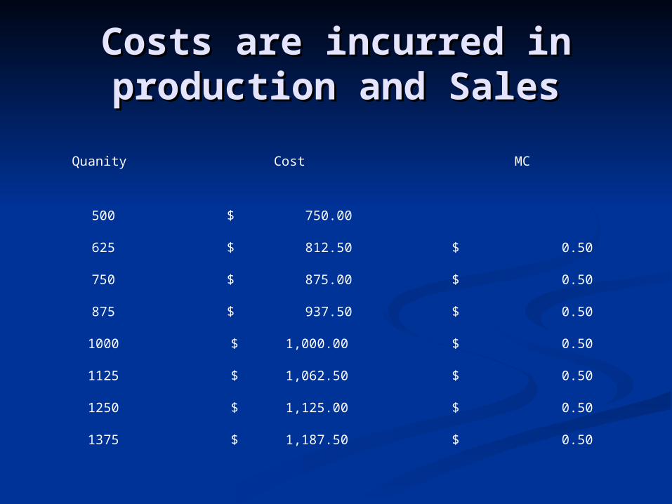
Costs are incurred in Costs are incurred in production and Salesproduction and Sales
Quanity Cost MC
500 $ 750.00
625 $ 812.50 $ 0.50
750 $ 875.00 $ 0.50
875 $ 937.50 $ 0.50
1000 $ 1,000.00 $ 0.50
1125 $ 1,062.50 $ 0.50
1250 $ 1,125.00 $ 0.50
1375 $ 1,187.50 $ 0.50
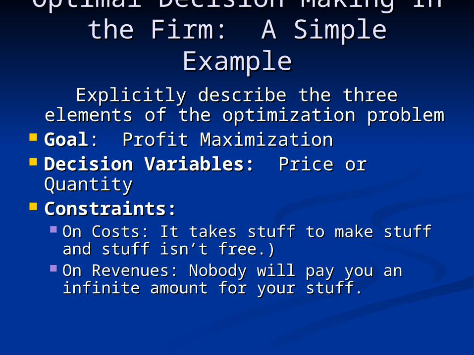
Optimal Decision Making In Optimal Decision Making In the Firm: A Simple Examplethe Firm: A Simple Example
Explicitly describe the three elements Explicitly describe the three elements of the optimization problemof the optimization problem
GoalGoal: Profit Maximization: Profit Maximization Decision Variables: Decision Variables: Price or Price or
QuantityQuantity Constraints:Constraints:
On Costs: It takes stuff to make stuff and On Costs: It takes stuff to make stuff and stuff isn’t free.)stuff isn’t free.)
On Revenues: Nobody will pay you an On Revenues: Nobody will pay you an infinite amount for your stuff.infinite amount for your stuff.
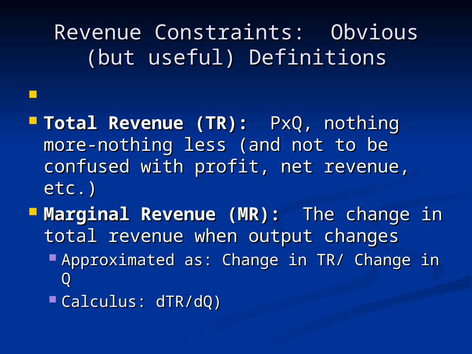
Revenue Constraints: Obvious (but Revenue Constraints: Obvious (but useful) Definitionsuseful) Definitions
Total Revenue (TR): Total Revenue (TR): PxQ, nothing PxQ, nothing
more-nothing less (and not to be more-nothing less (and not to be confused with profit, net revenue, etc.)confused with profit, net revenue, etc.)
Marginal Revenue (MR): Marginal Revenue (MR): The change The change in total revenue when output changesin total revenue when output changes Approximated as: Change in TR/ Change in Q Approximated as: Change in TR/ Change in Q Calculus: dTR/dQ)Calculus: dTR/dQ)
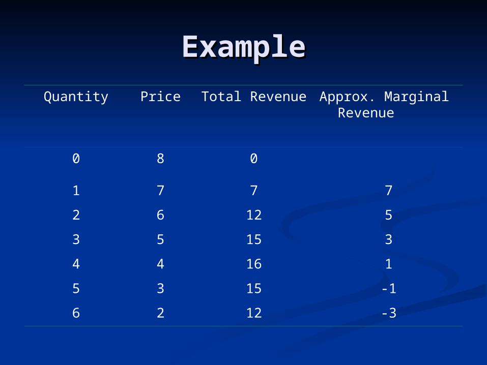
ExampleExample
Quantity Price Total Revenue Approx. Marginal Revenue
0 8 0
1 7 7 7
2 6 12 5
3 5 15 3
4 4 16 1
5 3 15 -1
6 2 12 -3

Putting it togetherPutting it together
Price Quanity Revenue MR Cost MC Profit
$ 4.00 500 $ 2,000.00 $ 750.00 $ 1,250.00
$ 3.75 625 $ 2,343.75 $ 2.75 $ 812.50 $ 0.50 $ 1,531.25
$ 3.50 750 $ 2,625.00 $ 2.25 $ 875.00 $ 0.50 $ 1,750.00
$ 3.25 875 $ 2,843.75 $ 1.75 $ 937.50 $ 0.50 $ 1,906.25
$ 3.00 1,000 $ 3,000.00 $ 1.25 $ 1,000.00 $ 0.50 $ 2,000.00
$ 2.75 1,125 $ 3,093.75 $ 0.75 $ 1,062.50 $ 0.50 $ 2,031.25
$ 2.50 1,250 $ 3,125.00 $ 0.25 $ 1,125.00 $ 0.50 $ 2,000.00
$ 2.25 1,375 $ 3,093.75 $(0.25) $ 1,187.50 $ 0.50 $ 1,906.25

Why Is the Optimal Q=1,125Why Is the Optimal Q=1,125
For all Q less than this, MR<MC, meaning an For all Q less than this, MR<MC, meaning an increase in output would raise revenue by increase in output would raise revenue by more than costs. more than costs.
For all Q greater than this MR<MC, meaning For all Q greater than this MR<MC, meaning an increase in output would raise revenue by an increase in output would raise revenue by less than the increase in costs. less than the increase in costs.
This is such an important conclusion, it This is such an important conclusion, it should be stated formally as should be stated formally as Necessary Necessary Condition for Profit Maximization: Condition for Profit Maximization: If you If you produce, produce the Q such that produce, produce the Q such that MR=MC.MR=MC.

Thinking about Thinking about optimization this way helps optimization this way helps understand two important understand two important
(related) principles(related) principles Fixed Costs Don’t matter (at least to Fixed Costs Don’t matter (at least to the optimal solution)the optimal solution)
Anything the “unnaturally” distorts Anything the “unnaturally” distorts marginal costs leads to a reduction marginal costs leads to a reduction in the optimal amount that can be in the optimal amount that can be achievedachieved
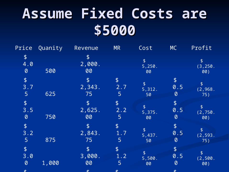
Assume Fixed Costs are Assume Fixed Costs are $5000$5000
Price Quanity Revenue MR Cost MC Profit
$ 4.00 500 $ 2,000.00 $ 5,250.00 $ (3,250.00)
$ 3.75 625 $ 2,343.75 $ 2.75 $ 5,312.50 $ 0.50 $ (2,968.75)
$ 3.50 750 $ 2,625.00 $ 2.25 $ 5,375.00 $ 0.50 $ (2,750.00)
$ 3.25 875 $ 2,843.75 $ 1.75 $ 5,437.50 $ 0.50 $ (2,593.75)
$ 3.00 1,000 $ 3,000.00 $ 1.25 $ 5,500.00 $ 0.50 $ (2,500.00)
$ 2.75 1,125 $ 3,093.75 $ 0.75 $ 5,562.50 $ 0.50 $ (2,468.75)
$ 2.50 1,250 $ 3,125.00 $ 0.25 $ 5,625.00 $ 0.50 $ (2,500.00)
$ 2.25 1,375 $ 3,093.75 $(0.25) $ 5,687.50 $ 0.50 $ (2,593.75)
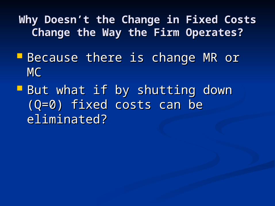
Why Doesn’t the Change in Fixed Costs Why Doesn’t the Change in Fixed Costs Change the Way the Firm Operates?Change the Way the Firm Operates?
Because there is change MR or MCBecause there is change MR or MC But what if by shutting down (Q=0) But what if by shutting down (Q=0)
fixed costs can be eliminated?fixed costs can be eliminated?
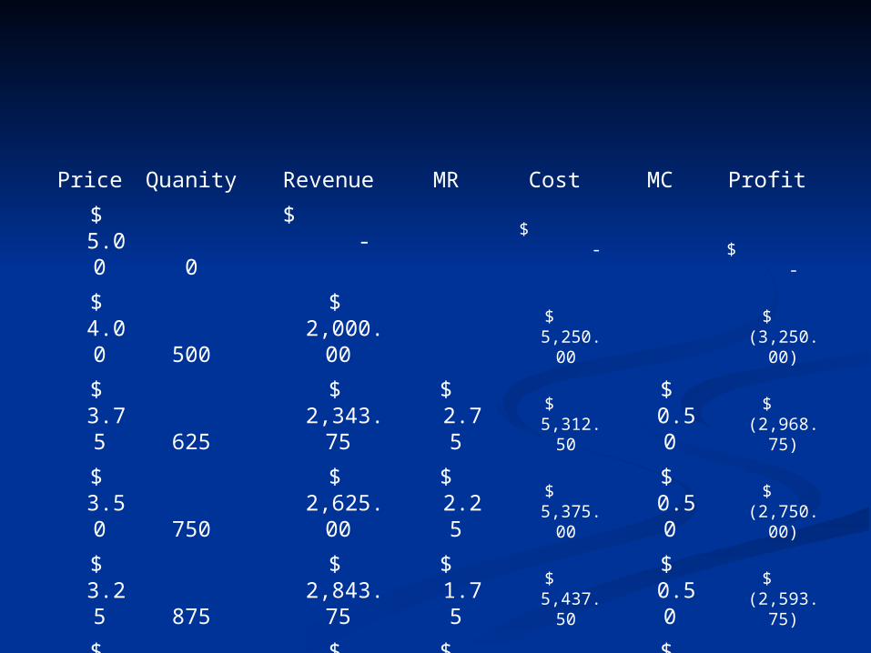
Price Quanity Revenue MR Cost MC Profit
$ 5.00 0 $ - $ - $ -
$ 4.00 500 $ 2,000.00 $ 5,250.00 $ (3,250.00)
$ 3.75 625 $ 2,343.75 $ 2.75 $ 5,312.50 $ 0.50 $ (2,968.75)
$ 3.50 750 $ 2,625.00 $ 2.25 $ 5,375.00 $ 0.50 $ (2,750.00)
$ 3.25 875 $ 2,843.75 $ 1.75 $ 5,437.50 $ 0.50 $ (2,593.75)
$ 3.00 1,000 $ 3,000.00 $ 1.25 $ 5,500.00 $ 0.50 $ (2,500.00)
$ 2.75 1,125 $ 3,093.75 $ 0.75 $ 5,562.50 $ 0.50 $ (2,468.75)
$ 2.50 1,250 $ 3,125.00 $ 0.25 $ 5,625.00 $ 0.50 $ (2,500.00)

Anything that “unnaturally” distorts marginal Anything that “unnaturally” distorts marginal costs leads to a reduction in the optimal costs leads to a reduction in the optimal
amount that can be achievedamount that can be achieved
Remember we saw that charging a per unit fee Remember we saw that charging a per unit fee reduced the combined profits. Now we know why.reduced the combined profits. Now we know why.
The tracks had control of the retail price and hence The tracks had control of the retail price and hence the sales volume.the sales volume.
The per unit fee was reflected in the sales price, but it The per unit fee was reflected in the sales price, but it didn’t represent a “real” cost. It appeared real didn’t represent a “real” cost. It appeared real enough to the tracks but it didn’t represent any actual enough to the tracks but it didn’t represent any actual expenditure, it was just a transfer from one division to expenditure, it was just a transfer from one division to the other. Thus it caused the tracks to raise the price the other. Thus it caused the tracks to raise the price of the programs beyond the optimal amount.of the programs beyond the optimal amount. In other words, the tracks were led to believe that there was In other words, the tracks were led to believe that there was
a variable cost (beyond the printing costs) a variable cost (beyond the printing costs) Can you think of other examples where firms make Can you think of other examples where firms make
this mistake?this mistake?

Everything you ever needed to know Everything you ever needed to know about calculus to solve optimization about calculus to solve optimization
problems in economicsproblems in economics Consider the simple functionConsider the simple function
y=6x-x2y=6x-x2 If we calculate the value of y for If we calculate the value of y for
various values of x, we getvarious values of x, we get
x 1 2 3 4 5
y 5 8 9 8 5
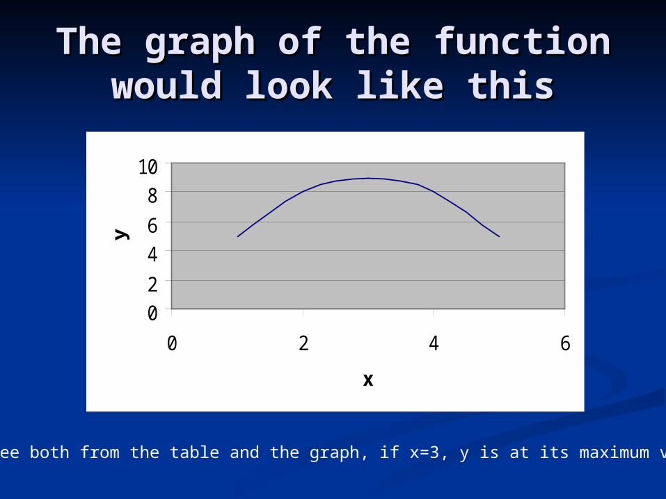
The graph of the function The graph of the function would look like thiswould look like this
0
2
4
6
8
10
0 2 4 6
x
y
As you can see both from the table and the graph, if x=3, y is at its maximum value.
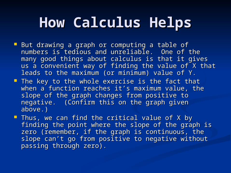
How Calculus HelpsHow Calculus Helps But drawing a graph or computing a table of But drawing a graph or computing a table of
numbers is tedious and unreliable. One of the many numbers is tedious and unreliable. One of the many good things about calculus is that it gives us a good things about calculus is that it gives us a convenient way of finding the value of X that leads to convenient way of finding the value of X that leads to the maximum (or minimum) value of Y.the maximum (or minimum) value of Y.
The key to the whole exercise is the fact that when a The key to the whole exercise is the fact that when a function reaches it’s maximum value, the slope of function reaches it’s maximum value, the slope of the graph changes from positive to negative. the graph changes from positive to negative. (Confirm this on the graph given above.) (Confirm this on the graph given above.)
Thus, we can find the critical value of X by finding Thus, we can find the critical value of X by finding the point where the slope of the graph is zero the point where the slope of the graph is zero (remember, if the graph is continuous, the slope (remember, if the graph is continuous, the slope can’t go from positive to negative without passing can’t go from positive to negative without passing through zero). through zero).

Now- and here’s where the calculus comes Now- and here’s where the calculus comes in—the in—the derivativederivative of a function is nothing of a function is nothing more than a very precise measurement of more than a very precise measurement of the slope of the graph of the function. the slope of the graph of the function.
Thus, if we can find the value of X at which Thus, if we can find the value of X at which the derivative of the function is zero, we will the derivative of the function is zero, we will have identified the optimal value of the have identified the optimal value of the function. function.
If this were a math class, we’d spend several If this were a math class, we’d spend several lectures studying exactly what is meant by a lectures studying exactly what is meant by a derivative of a function and we’d end up derivative of a function and we’d end up with some rules for finding a derivative. with some rules for finding a derivative.
But since this isn’t a math class, we’ll go But since this isn’t a math class, we’ll go straight to the rules (especially since we straight to the rules (especially since we only need a few of them and they’re very only need a few of them and they’re very easy to remember.)easy to remember.)

Rules for finding derivativesRules for finding derivatives
The derivative of a constant is zero. The derivative of a constant is zero. If Y=C for all X, then dY/dX=0If Y=C for all X, then dY/dX=0 (Which makes sense, since the graph of Y=C (Which makes sense, since the graph of Y=C
is a flat line and thus has a slope of zero). is a flat line and thus has a slope of zero). The derivative of a linear function is the The derivative of a linear function is the
coefficient (the thing multiplied by the coefficient (the thing multiplied by the variable)variable) If Y=bX, then dY/dX=bIf Y=bX, then dY/dX=b
(Which makes sense, since the slope of (Which makes sense, since the slope of this function is just the coefficient.)this function is just the coefficient.)
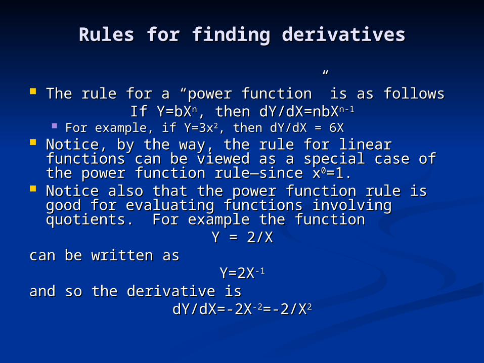
Rules for finding derivativesRules for finding derivatives
The rule for a “power function” is as followsThe rule for a “power function” is as followsIf Y=bXIf Y=bXnn, then dY/dX=nbX, then dY/dX=nbXn-1n-1
For example, if Y=3xFor example, if Y=3x22, then dY/dX = 6X, then dY/dX = 6X Notice, by the way, the rule for linear functions Notice, by the way, the rule for linear functions
can be viewed as a special case of the power can be viewed as a special case of the power function rule—since xfunction rule—since x00=1. =1.
Notice also that the power function rule is good Notice also that the power function rule is good for evaluating functions involving quotients. For for evaluating functions involving quotients. For example the functionexample the function
Y = 2/XY = 2/Xcan be written ascan be written as
Y=2XY=2X-1-1
and so the derivative isand so the derivative isdY/dX=-2XdY/dX=-2X-2-2=-2/X=-2/X22

Rules for finding derivativesRules for finding derivatives
The derivative of a function that is the The derivative of a function that is the sum of several functions is the sum of the sum of several functions is the sum of the derivatives of those functionsderivatives of those functions If Y=f(x)+g(x), If Y=f(x)+g(x), then then dY/dX=df(x)/dx+dg(x)/dxdY/dX=df(x)/dx+dg(x)/dx
By combining these rules we can find the By combining these rules we can find the derivative of any polynomial.derivative of any polynomial. If Y=a + bx + cx2+…+dxn,If Y=a + bx + cx2+…+dxn, thenthen dY/dX=b+2cX+…+ndXn-1dY/dX=b+2cX+…+ndXn-1

The derivative of the product of two The derivative of the product of two functions is as followsfunctions is as follows
If Y = f(x )g(x), If Y = f(x )g(x),
then then
dY/dX = f(x)[dg(x)/dx]+g(x)[df(x)/dx]dY/dX = f(x)[dg(x)/dx]+g(x)[df(x)/dx]
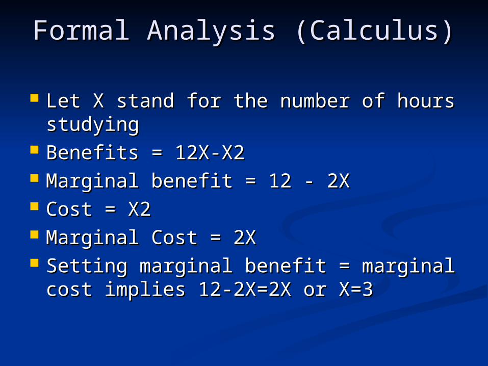
Formal Analysis (Calculus)Formal Analysis (Calculus)
Let X stand for the number of hours Let X stand for the number of hours studyingstudying
Benefits = 12X-X2Benefits = 12X-X2 Marginal benefit = 12 - 2XMarginal benefit = 12 - 2X Cost = X2Cost = X2 Marginal Cost = 2XMarginal Cost = 2X Setting marginal benefit = marginal Setting marginal benefit = marginal
cost implies 12-2X=2X or X=3cost implies 12-2X=2X or X=3