Lecture 1b-Introduction to Synthesis Modeltitan.fsb.hr/~pprebeg/optkon/literatura/lec1b.pdf · LECTURE 1b SYNTHESIS MODEL Optimization methods and solution strategies Design wheel

Lecture 1b 3/13/2007

Optimization of Thin Walled Structures Slide No: 1/34

LECTURE 1b SYNTHESIS MODEL Optimization methods and solution strategies

Design wheel



Ship design spiral

Circular component: Radial component: accuracy level



Structure design spiral



Structural design parameters include

scantlings, material (e.g. layer characteristics and orientation in

composites), topology and geometry of the structure.

Since the latter two are usually fixed, except in shape optimization problems, the first two are commonly taken as free design variables.



Design quality measures are defined by using a set of design criteria functions (mappings) for :

structural cost,

weight

safety evaluations.

Principles of design would require that for a good design:

(Axiom I), the qualities, should be as much as possible uncoupled with respect to parameters,

(Axiom II) the information content describing good design

should be minimal (simplicity).



‘Best’ design(s) can be determined by three classical ways of decision making

lexicographical ordering of priorities (method selects

among the ‘best’ candidates regarding the first priority those that are the ‘best’ regarding second priority, etc).;

goal seeking (construction of metric or ‘distance’ measure

to the target design);

construction of value function (combination of attribute functions as ultimate quality measure).



Description of sets/spaces and transformations

Figs. 1a-d give visual insight into concepts encountered in the realistic DS formulations

(dominance, fuzziness, metrics).



Figure 1

lk∈L

l2*

lP l2

l1P

l2P

l∞P

l22

l∞2

l12

l3 l4 l1k

Design-k 2 3 4 51 6

MN

l2k=v2(mk)

l1k=v1(mk)

l∞k=v3(mk)

LN

l2*

l1*

l∞*

preferred d i

x1

x2 gi(xk)≥0

x1L x1

U

X≥

XN

DESIGN (r -1: L→X≥)

EVALUATION (r: X≥ →L)

x2

xP

(a) (d)

a: X

≥ → Y

≥

v: M

N →

LN

m2



ABCD

E

PG

H y1

y2

y1H

A BC D

E

Gm2

m1

P

m2

y2

w21

m1

w1

1

P

m*

l1=const. l2=const.

U1(y1) m1

P

y1P

U2(y2)Y≥

hi(yk)≥0

y*

YN

YN

y2*

y1*

MN

a: X

≥ → Y

≥

u: Y≥ → M≥

v: M

N →

LN

(b) (b1)

(b2) (c)

l∞=const.P

idealdesign

y2p

m2P

u2(y2)=w2U2(y2)

u1(y1)=w1U1(y1)

M≥



Design space

Design space X- is spanned by the free design variables xi, i=1,.., nv. (see Fig. 1a)

Each design k is represented as a point xk={xi} (e.g. x2 or xP) in

this space.

Some of the variables are discrete (no. of stiffeners, standard profiles). That could strongly influence problem formulation.



Design space

Designs in subspace of feasible designs X≥ satisfy:

failure criteria gi(x) ≥ 0 production requirements, functionality requirements, min-max bounds xi

L and xiU

other constraints.



Design space

Note that X≥ may be convex (line connecting two designs lies in X≥) or non-convex as in Fig. 1a.

Note also that it can be multiply connected (containing holes for e.g. resonance avoidance in vibration problems) and



Dimensionality

Dimensionality of the problem is given by the number of variables nv.

For concept structural design nv~40.

Preliminary/Initial design would require nv~200/1000.

The "curse of dimensionality". Most of design variables are

structural scantlings and spacing of girders on 2D (midship section, bulkheads) or 3D structures.

Dimensionality is higher (100-1000) only in few works.

Constraints gi(.)≥ 0 are either global and local strength formulae or Rules. Structural response is calculated using FEM or analytical methods.



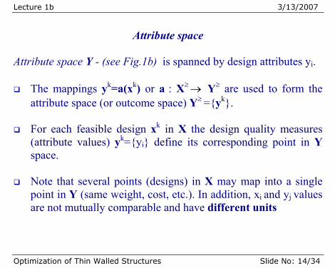
Attribute space

Attribute space Y - (see Fig.1b) is spanned by design attributes yi.

The mappings yk=a(xk) or a : X≥ → Y≥ are used to form the attribute space (or outcome space) Y≥ ={yk}.

For each feasible design xk in X the design quality measures

(attribute values) yk={yi} define its corresponding point in Y space.

Note that several points (designs) in X may map into a single

point in Y (same weight, cost, etc.). In addition, xi and yj values are not mutually comparable and have different units



Attribute and Design spaces

X and Y are not metric spaces i.e. there is no distance measure

among designs.

The comparison of designs is possible only within single variable xi or attribute yj.

If direction is selected for the quality improvement (e.g.

minimal cost, maximal safety) attributes are transferred to objectives.

’Ideal’ y* is a design (usually infeasible) with the coordinates

of the best achieved quality for each objective.



Concept of non-dominance (Figs. 1a, 1b):

The subspace YN of non-dominated or Pareto optimal or efficient designs can be identified when designer’s preference structure is applied to designs (points) in Y≥.

Only those designs (usually only a small fraction of feasible designs) are of interest to designer since they dominate all

other feasible designs.



Concept of non-dominance

Preference is a binary relation stating that design yi is preferred to design yj.

“Better set” can be defined with respect to given design y0 if

all its elements are preferred to y0.

Conversely, the “worse set” can be formed containing all designs that are worse than y0 in all attributes i.e. dominated by it.

For the preference ‘more is better’ it is easy to visualize the

“worse set” to e.g. design yP (see Fig. 1b) as a negative cone with an apex in yP containing points left of line y1

P and below the line y2

P.



Finally, the set of non-dominated designs YN is defined as a set of designs that have no “better set“, hence they are not dominated by any design.

Alternatively, design is non-dominated if it is better than any

other design in Y≥ in at least one objective.

Points in YN have their design variable description in XN (see Fig. 1a).



Inclusion of subjectivity Inclusion of subjectivity- see Figs. 1b1 and 1b2 is basic to realistic decision-making. It implies:

Subjective comparison of various designs can be performed using fuzzy functions Ui(yi).

Membership grade (satisfaction level) μi=Ui(yi) has range 0-1

(see dotted line).

In vibration problems this function may consist of e.g. series of the inverse bell shaped functions centered at excitation frequencies (μi=0 for design in resonance). Concept is widely used in DSP.



Inclusion of subjectivity

Determination of subjective importance of different attributes can be based on weighting factors wi (P).

The bi-attribute preference matrix P=[pij] contains ratios of

subjective importance of attribute yi compared to yj..

Combination of subjectivities for attribute i can be achieved as e.g. product

ui(yi)= wi(P) Ui(yi) .



Inclusion of subjectivity Subjective metric space- (see Fig. 1c) is formed by using mappings

u : Y≥ → M≥

There now exists possibility of the introduction of metric

(distance measure) since all attribute values

mi = ui(yi) m = {mi}

are normalized and scaled to their relative importance.

Subjective criteria functions u enable natural ‘more is better’ preference structure and make it even easier to filter the subset of non-dominated designs MN from M≥ and then generate corresponding YN and XN.



Value functions

Value functions v (utility fn. see Yu, 1985) are defined as mappings li =vi (m).

Vector lk={li} contains values obtained from different value functions including in its formulation the subjectivity of designer and others involved in DM.

The iso-value contours li = const. can be visualized in M-

space.

These contours (like in geography), may exhibit multiple peaks. Some of those peaks correspond to local minima/maxima and some are global i.e. best for the entire M≥.

Note that optimum in constrained problems is often achieved

on boundaries of feasible region.



Distance norms (metrics) Distance norms (metrics) Lp are commonly used as value functions.

Distance to the specified target design m*(e.g. ideal design) is given by standard expression

Lp(mk) = [∑|mik-mi

*|p]1/p .

Exponent p in the norm definition is taken as 1 Metropolitan n. 2 Euclidean n. ∞ Chebisev n.



Distance norms (metrics)

The iso-value contours for given distance norms are (see Fig.1c):

(1) straight lines ∑mi=const for L1, (2) circles around m* for L2 (3) mi=const for L∞ .

The non-dominated design for min L∞ (marked ■) can be linked to so-called ‘fuzzy optimum’ i.e. a design for which the minimal mi

in mk is maximal.



Selection Selection of preferred design-see Fig. 1d :

Final selection of preferred design P: dP= {xP, yP, mP, lP} requires the calculation of values lk for all designs in MN.

Since final decision is made only on the basis of lk, all li can be

put on same axis for each design k.

A set of parallel axis for all candidate designs can be displayed to facilitate final subjective decision.

Parallel axes can also correspond to all li. Lines connecting

specific designs on all axes are used to facilitate ranking of designs.



Sensitivity analysis, Robustness and Stochastic Characteristics:

For technical systems the existence of solution is often guaranteed but not its uniqueness and stability.

Many parameters, held constant during optimization process,

are subject to uncertainties causing variations of the values in the criteria set Y and/or violation of constraints (unfeasible designs).



Robustness Robustness is defined as insensitivity (or stability) with respect to such changes.



Design mapping-see Figs.1a,1d :

Composite value function li =ri(xk), built from subjective criteria functions ri(xk) ≡ vi (u(a(xk))), maps the feasible designs subspace X≥ into the designer's selection set L.

The obtained values lk (cost, weight, etc.) are used for the final evaluation of the design.



Design mapping

The described mapping r : X≥ → L is called evaluation mapping.

But in the design process the designer’s task is to determine values of design variables xA for given aspired values lA of cost, weight, etc.

Therefore the construction of the inverse or design mapping r-1 : lA → X≥, that maps designer’s aspirations to design parameters, is the essence of design.



Examples of Attribute space (Evans 1974)









Examples of design problem definition regarding 4 ship types from Lecture 1a.

MODELS VARIABLES PARAMETERS ATTRIBUTES CONSTRAINTS

SCANTLINGS COST C.S. RULES

MATERIAL

TRANSV. STRUC. (CLASSIC, HINGE)

SAFETY ULT. STRENGTH 1

CAR CARRIER

STIFFENING TYPE PILLAR SYST. DWT CLEARANCES

SCANTLINGS BRIDGE STRUCT COST C.S. RULES

MATERIAL STERN STRUCT SAFETY ULT. STRENGTH 2

LIVESTOCK CARRIER

STIFFENING TYPE PILLAR SYST. MAINTENANCE RACKING

SCANTLINGS RECES POSITION COST C.S. RULES

MATERIAL TBKHD, LBKHD SAFETY ULT. STRENGTH 3

CRUISE SHIP

STIFFENING TYPE SIDE OPENINGS VCG WINDOWS

SCANTLINGS DECKHOUSE LGT COST C.S. RULES

MATERIAL DH. MATERIAL SAFETY ULT. STRENGTH 4

TANK-CAR CARRIER

STIFFENING TYPE DH. LAYOUT ROBUSTNESS CLEARANCES



Lecture1c MAESTRO PRESENTATION

Documents

Lecture 1b-Introduction to Synthesis Modeltitan.fsb.hr/~pprebeg/optkon/literatura/lec1b.pdf · LECTURE 1b SYNTHESIS MODEL Optimization methods and solution strategies Design wheel