Lecture 19 More on Hollow Waveguides

Lecture 19

More on Hollow Waveguides

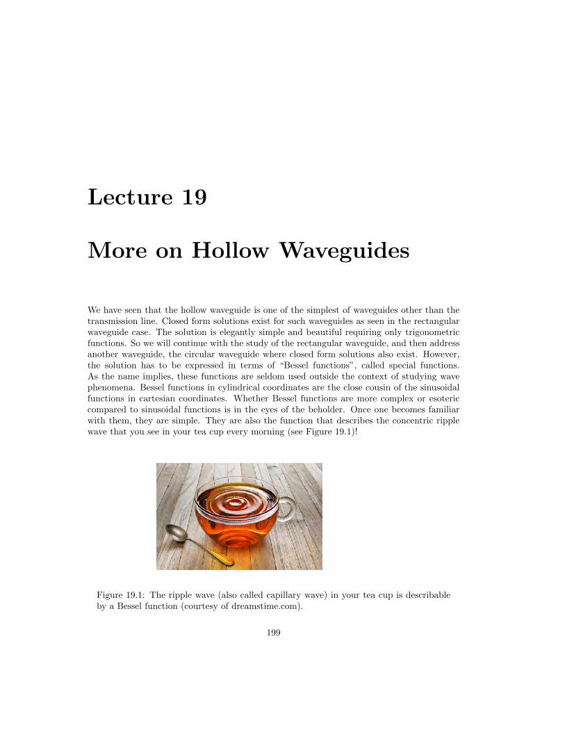
We have seen that the hollow waveguide is one of the simplest of waveguides other than thetransmission line. Closed form solutions exist for such waveguides as seen in the rectangularwaveguide case. The solution is elegantly simple and beautiful requiring only trigonometricfunctions. So we will continue with the study of the rectangular waveguide, and then addressanother waveguide, the circular waveguide where closed form solutions also exist. However,the solution has to be expressed in terms of “Bessel functions”, called special functions.As the name implies, these functions are seldom used outside the context of studying wavephenomena. Bessel functions in cylindrical coordinates are the close cousin of the sinusoidalfunctions in cartesian coordinates. Whether Bessel functions are more complex or esotericcompared to sinusoidal functions is in the eyes of the beholder. Once one becomes familiarwith them, they are simple. They are also the function that describes the concentric ripplewave that you see in your tea cup every morning (see Figure 19.1)!

Figure 19.1: The ripple wave (also called capillary wave) in your tea cup is describableby a Bessel function (courtesy of dreamstime.com).

199

200 Electromagnetic Field Theory

19.1 Rectangular Waveguides, Contd.

We have seen the mathematics for the TE modes of a rectangular waveguide. We shall studythe TM modes and the modes of a circular waveguide in this lecture.

19.1.1 TM Modes (Ez 6= 0, E Modes or TMz Modes)

These modes are not the exact dual of the TE modes because of the boundary conditions.The dual of a PEC (perfect electric conducting) wall is a PMC (perfect magnetic conducting)wall. However, the previous exercise for TE modes can be repeated for the TM modes withcaution on the boundary conditions. The scalar wave function (or eigenfunction/eigenmode)for the TM modes, satisfying the homogeneous Dirichlet (instead of Neumann)1 boundarycondition with (Ψes(rs) = 0) on the entire waveguide wall is

Ψes(x, y) = A sin(mπax)

sin(nπby)

(19.1.1)

where βx = mπa and βy = nπ

b . Here, sine functions are chosen for the standing waves, andthe chosen values of βx and βy ensure that the boundary condition is satisfied on the x = aand y = b walls. Neither of the m and n can be zero, lest Ψes(x, y) = 0, or the field is zero.Hence, both m > 0, and n > 0 are needed. Thus, the lowest TM mode is the TM11 mode.Thinking of this as an eigenvalue problem, then the eigenvalue is

β2s = β2

x + β2y =

(mπa

)2

+(nπb

)2

(19.1.2)

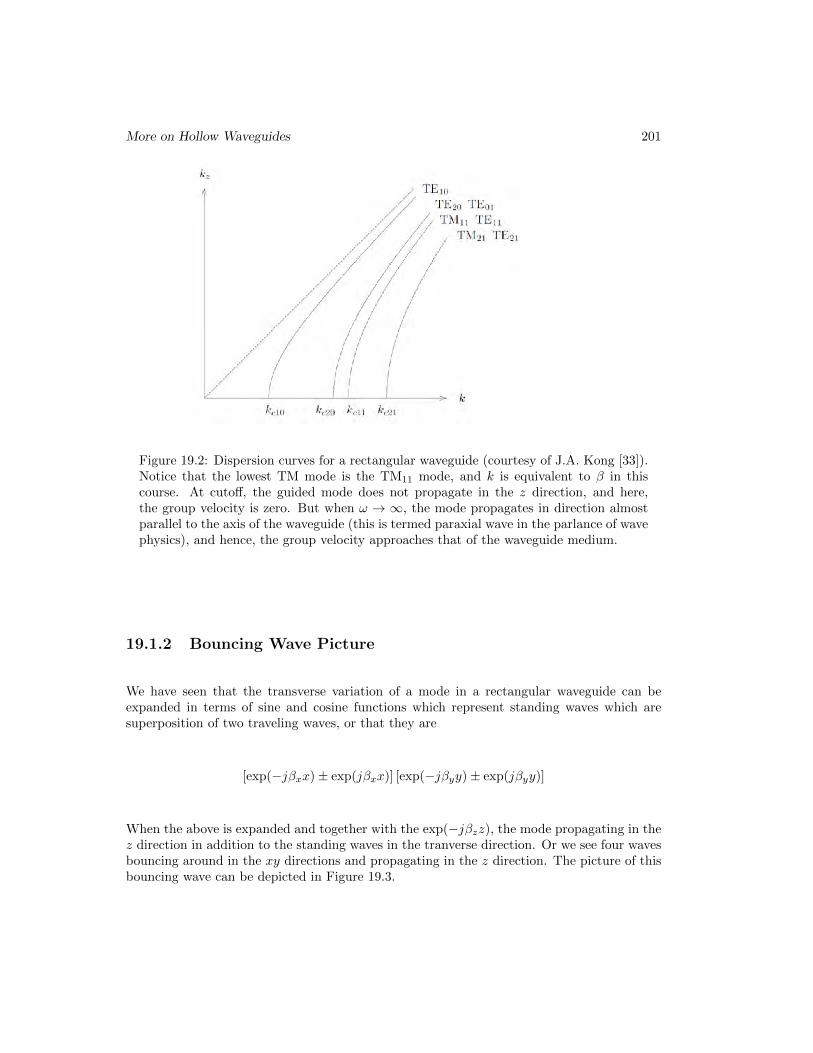
which is the same as the TE case. Therefore, the corresponding cutoff frequencies and cutoffwavelengths for the TMmn modes are the same as the TEmn modes. Also, these TE andTM modes are degenerate when they share the same eigevalues. Moreover, the lowest modes,TE11 and TM11 modes have the same cutoff frequency. Figure 19.2 shows the dispersioncurves for different modes of a rectangular waveguide. Notice that the group velocities of allthe modes are zero at cutoff, and then the group velocities approach that of the waveguidemedium as frequency becomes large. These observations can be explained physically as westudy the bouncing-wave picture next.

1Again, “homogeneous” here means “zero”.

More on Hollow Waveguides 201

Figure 19.2: Dispersion curves for a rectangular waveguide (courtesy of J.A. Kong [33]).Notice that the lowest TM mode is the TM11 mode, and k is equivalent to β in thiscourse. At cutoff, the guided mode does not propagate in the z direction, and here,the group velocity is zero. But when ω → ∞, the mode propagates in direction almostparallel to the axis of the waveguide (this is termed paraxial wave in the parlance of wavephysics), and hence, the group velocity approaches that of the waveguide medium.

19.1.2 Bouncing Wave Picture

We have seen that the transverse variation of a mode in a rectangular waveguide can beexpanded in terms of sine and cosine functions which represent standing waves which aresuperposition of two traveling waves, or that they are

[exp(−jβxx)± exp(jβxx)] [exp(−jβyy)± exp(jβyy)]

When the above is expanded and together with the exp(−jβzz), the mode propagating in thez direction in addition to the standing waves in the tranverse direction. Or we see four wavesbouncing around in the xy directions and propagating in the z direction. The picture of thisbouncing wave can be depicted in Figure 19.3.


Figure 19.3: The waves in a rectangular waveguide can be thought of as bouncing wavesoff the four walls as they propagate in the z direction out of the paper.

19.1.3 Field Plots

Given the knowledge of the vector pilot potential of a waveguide, one can derive all the fieldcomponents. For example, for the TE modes, if we know Ψh(r), then

E = ∇× zΨh(r), H = −∇×E/(jωµ) (19.1.3)

Then all the electromagnetic field of a waveguide mode can be found, and similarly for TMmodes.

Plots of the fields of different rectangular waveguide modes are shown in Figure 19.4.Notice that for higher m’s and n’s, with βx = mπ/a and βy = nπ/b, the corresponding βxand βy are larger with higher spatial frequencies. Thus, the transverse spatial wavelengths are

getting shorter. Also, since βz =√β2 − β2

x − β2y , higher frequencies are needed to make βz

real in order to propagate the higher order modes or the high m and n modes in a rectangularwaveguide.

Notice also how the electric field and magnetic field curl around each other. Since ∇×H =jωεE and ∇ × E = −jωµH, they do not curl around each other “immediately” but with aπ/2 phase delay due to the jω factor. Therefore, the E and H fields do not curl around eachother at one location, but at a displaced location due to the π/2 phase difference. This isshown in Figure 19.5.


Figure 19.4: Transverse field plots of different modes in a rectangular waveguide (courtesyof Andy Greenwood. Original plots published in Lee, Lee, and Chuang, IEEE T-MTT,33.3 (1985): pp. 271-274. [127]).

Figure 19.5: Field plot of a mode propagating in the z direction of a rectangular waveg-uide. Notice that the E and H fields do not exactly curl around each other.


19.2 Circular Waveguides

Another waveguide where closed-form solutions can be easily obtained is the circular hollowwaveguide as shown in Figure 19.6, but they involve the use of Bessel functions.

Figure 19.6: Schematic of a circular waveguide in cylindrical coordinates. It is one of theseparable coordinate systems.

19.2.1 TE Case

For a circular waveguide, it is best first to express the Laplacian operator, ∇s2 = ∇s · ∇s, incylindrical coordinates. The second term ∇s is a gradient operator while the first term ∇s·is a divergence operator: they have different physical meanings. Formulas for grad and divoperators are given in many text books [33,128]. Doing a table lookup,

∇sΨ = ρ∂

∂ρΨ + φ

1

ρ

∂

∂φ

∇s ·A =1

ρ

∂

∂ρρAρ +

1

ρ

∂

∂φAφ

Then (∇s2 + βs

2)

Ψhs =

(1

ρ

∂

∂ρρ∂

∂ρ+

1

ρ2

∂2

∂φ2+ βs

2

)Ψhs(ρ, φ) = 0 (19.2.1)

The above is the partial differential equation for field in a circular waveguide. It is an eigen-value problem where β2

s is the eigenvalue, and Ψhs(rs), where rs = ρρ+φφ, is the eigenfunction(equivalence of an eigenvector). Using separation of variables, we let

Ψhs(ρ, φ) = Bn(βsρ)e±jnφ (19.2.2)


Then ∂2

∂φ2 → −n2, and (19.2.1) simplifies to an ordinary differential equation which is(1

ρ

d

dρρd

dρ− n2

ρ2+ βs

2

)Bn(βsρ) = 0 (19.2.3)

Here, dividing the above equation by β2s , we can let βsρ in (19.2.2) and (19.2.3) be x. Then

the above can be rewritten as(1

x

d

dxxd

dx− n2

x2+ 1

)Bn(x) = 0 (19.2.4)

The above is known as the Bessel equation whose solutions are special functions denoted asBn(x).2

These special functions are Jn(x), Nn(x), H(1)n (x), and H

(2)n (x) which are called Bessel,

Neumann, Hankel function of the first kind, and Hankel function of the second kind, respec-tively, where n is their order, and x is their argument.3 Since this is a second order ordinarydifferential equation, it has only two independent solutions. Therefore, two of the four com-monly encountered solutions of Bessel equation are independent. Thus, they can be expressedin terms of each other. Their relationships are shown below:4

Bessel, Jn(x) =1

2[Hn

(1)(x) +Hn(2)(x)] (19.2.5)

Neumann, Nn(x) =1

2j[Hn

(1)(x)−Hn(2)(x)] (19.2.6)

Hankel–First kind, Hn(1)(x) = Jn(x) + jNn(x) (19.2.7)

Hankel–Second kind, Hn(2)(x) = Jn(x)− jNn(x) (19.2.8)

It can be shown that

Hn(1)(x) ∼

√2

πxejx−j(n+ 1

2 )π2 , x→∞ (19.2.9)

Hn(2)(x) ∼

√2

πxe−jx+j(n+ 1

2 )π2 , x→∞ (19.2.10)

They correspond to traveling wave solutions when x = βsρ → ∞. Since Jn(x) and Nn(x)are linear superpositions of these traveling wave solutions, they correspond to standing wavesolutions. Moreover, Nn(x), Hn

(1)(x), and Hn(2)(x) → ∞ when x → 0. Since the field

has to be regular when ρ → 0 at the center of the waveguide shown in Figure 19.6, theonly viable solution for the hollow waveguide, to be chosen from (19.2.5) to (19.2.9), is thatBn(βsρ) = AJn(βsρ). Thus for a circular hollow waveguide, the eigenfunction or mode is ofthe form

Ψhs(ρ, φ) = AJn(βsρ)e±jnφ (19.2.11)

2Studied by Friedrich Wilhelm Bessel, 1784-1846.3Some textbooks use Yn(x) for Neumann functions.4Their relations with each other are similar to those between exp(±jx), sin(x), and cos(x).


To ensure that the eigenfunction and the eigenvalue are unique, boundary condition for thepartial differential equation is needed. The homogeneous Neumann boundary condition,5 orthat ∂nΨhs = 0, on the PEC waveguide wall then translates to

d

dρJn(βsρ) = 0, ρ = a (19.2.12)

Defining Jn′(x) = d

dxJn(x),6 the above is the same as

Jn′(βsa) = 0 (19.2.13)

The above are the zeros of the derivative of Bessel function and they are tabulated in manytextbooks and handbooks.7 The m-th zero of Jn

′(x) is denoted to be βnm in many books.Plots of Bessel functions and their derivatives are shown in Figure 19.8, and some zeros ofBessel function and its derivative are also shown in Figure 19.9. With this knowledge, theguidance condition for a waveguide mode is then

βs = βnm/a (19.2.14)

for the TEnm mode. From the above, β2s can be obtained which is the eigenvalue of (19.2.1)

and (19.2.3). It is a constant independent of frequency.Using the fact that βz =

√β2 − β2

s , then βz will become pure imaginary if β2 is smallenough (or the frequency low enough) so that β2 < β2

s or β < βs. From this, the correspondingcutoff frequency (the frequency below which βz becomes pure imaginary) of the TEnm modeis

ωnm,c =1√µε

βnma

(19.2.15)

When ω < ωnm,c, the corresponding mode cannot propagate in the waveguide as βz becomespure imaginary. The corresponding cutoff wavelength is

λnm,c =2π

βnma (19.2.16)

By the same token, when λ > λnm,c, the corresponding mode cannot be guided by thewaveguide. It is not exactly precise to say this, but this gives us the heuristic notion that ifwavelength or “size” of the wave or photon is too big, it cannot fit inside the waveguide.

19.2.2 TM Case

The corresponding partial differential equation and boundary value problem for this case is(1

ρ

∂

∂ρρ∂

∂ρ+

1

ρ2

∂2

∂φ2+ βs

2

)Ψes(ρ, φ) = 0 (19.2.17)

5Note that “homogeneous” here means “zero” in math.6Note that this is a standard math notation, which has a different meaning in some engineering texts.7Notably, Abramowitz and Stegun, Handbook of Mathematical Functions [129]. An online version is

available at [130].


with the homogeneous Dirichlet boundary condition, Ψes(a, φ) = 0, on the waveguide wall.The eigenfunction solution is

Ψes(ρ, φ) = AJn(βsρ)e±jnφ (19.2.18)

with the boundary condition that Jn(βsa) = 0. The zeros of Jn(x) are labeled as αnm ismany textbooks, as well as in Figure 19.9; and hence, the guidance condition for the TMnm

mode is that

βs =αnma

(19.2.19)

where the eigenvalue for (19.2.17) is β2s which is a constant independent of frequency. With

βz =√β2 − β2

s , the corresponding cutoff frequency is

ωnm,c =1√µε

αnma

(19.2.20)

or when ω < ωnm,c, the mode cannot be guided. The cutoff wavelength is

λnm,c =2π

αnma (19.2.21)

with the notion that when λ > λnm,c, the mode cannot be guided.It turns out that the lowest mode in a circular waveguide is the TE11 mode. It is actually a

close cousin of the TE10 mode of a rectangular waveguide. This can be gathered by comparingtheir field plots: these modes morph into each other as we deform the shape of a rectangularwaveguide into a circular waveguide.

Figure 19.7: Side-by-side comparison of the field plots of the TE10 mode of a rectangularwaveguide versus that of the TE11 mode of a circular waveguide. If one is imaginativeenough, one can see that the field plot of one mode morphs into that of the other mode.Electric fields are those that have to end on the waveguide walls with n×E = 0.

Figure 19.8 shows the plots of Bessel function Jn(x) and its derivative J ′n(x). Tables inFigure 19.9 show the roots of J ′n(x) and Jn(x) which are important for determining the cutofffrequencies of the TE and TM modes of circular waveguides.


Figure 19.8: Plots of the Bessel function, Jn(x), and its derivatives J ′n(x). The zeros ofthese functions are used to find the eigenvalue β2

s of the problem, and hence, the guidancecondition. The left figure is for TM modes, while the right figure is for TE modes. Here,J ′n(x) = dJn(x)/dx [85].

Figure 19.9: Table 2.3.1 shows the zeros of J ′n(x), which are useful for determining theguidance conditions of the TEmn mode of a circular waveguide. On the other hand, Table2.3.2 shows the zeros of Jn(x), which are useful for determining the guidance conditionsof the TMmn mode of a circular waveguide [85].


Figure 19.10: Transverse field plots of different modes in a circular waveguide (courtesy ofAndy Greenwood. Original plots published in Lee, Lee, and Chuang [127]). The axiallysymmetric TE01 mode has the lowest loss, and finds a number of real-world applicationsas in radio astronomy.


Documents

Lecture 19 More on Hollow Waveguides