Lecture 17 Linear Algebra I - cs.brown.edu

Lecture 17Linear Algebra I

1

Outline

•Motivation•Linear equations, Linear systems

•Vectors•Length, Dot Product

•Matrices •Matrix Vector Product, Matrix Multiplication

•Solving systems of linear equations

2

Linear equations – circuit modeling

3

Equations for voltage and current are linear

If you know the voltages, the currents can be obtained by solving the following linear system

where the unknown are the currents (i’s)

Linear Equations

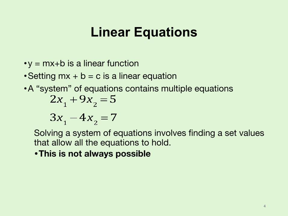
•y = mx+b is a linear function•Setting mx + b = c is a linear equation•A “system” of equations contains multiple equations

Solving a system of equations involves finding a set values that allow all the equations to hold. •This is not always possible

4

Systems of Equations

Examples

Linear Equations: y = mx + b•One solution•No solution• Infinite number of solutions

Disks in the plane (non-linear): (x - x0)^2 + (x - y0)^2 = r0•What are the possibilities?

5

Linear equations in Matrix Form

6

Example of linear equations

Can be written in matrix form

Or more symbolically as:

Where

Linear equations in Matrix Form

7

m linear equations with n variables:

Can be written in matrix form where

Matrices - Review

• A matrix consists of a rectangular array of elements represented by a single symbol e.g., A

• An individual entry of a matrix is an element e.g., a23 , can also write A23

8

Review (cont)

• A horizontal set of elements is called a row and a vertical set of elements is called a column.

• The first subscript of an element indicates the row while the second indicates the column.

• The size of a matrix is given as m rows by n columns, or simply m by n (or m x n).

• 1 x n matrices are row vectors.• m x 1 matrices are column vectors.

9

Matrix Operations

• isequal(A,B)Two matrices are considered equal if and only if every element in the first matrix is equal to every corresponding element in the second. This means the two matrices must be the same size.

• A+B, A-BMatrix addition and subtraction are performed by adding or subtracting the corresponding elements. This requires that the two matrices be the same size.

• A*cScalar matrix multiplication is performed by multiplying each element by the same scalar

10

Matrix-Vector multiplication

11

If A is an n-by-m matrix, and x is an m-by-1 vector, then the “product Ax” is a n-by-1 vector, whose i’th component is

=n-by-m

m-by-1 n-by-1

=n-by-m

m-by-1 n-by-1

Ax as linear combination of columns of A

12

Example norms

13

By default the L2 (Euclidian) norm

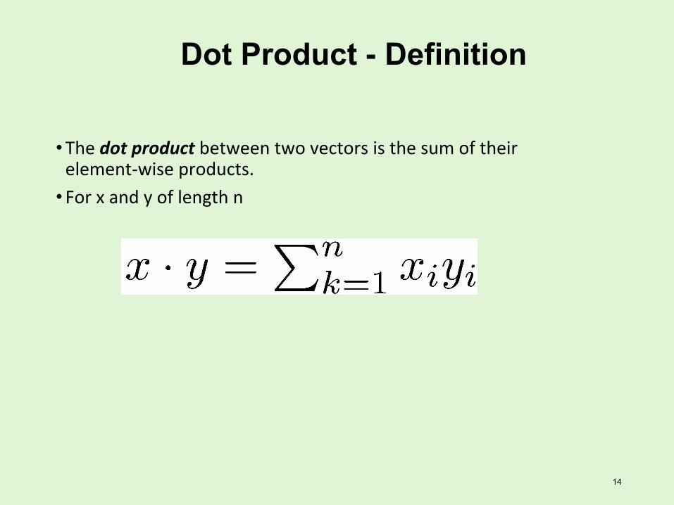
Dot Product - Definition

•

•

14

Dot product in MATLAB

15

Use dot command directly

The dot product operation on vectors:

Or transpose a and then matrix multiply by b (more about this in a moment).

Dot Product – Geometric interpretation

The Dot Product equivalent to

where and are the lengths (L2 norm) of x and y, and is the angle between vectors x and y.

Remark: Derivation can be done in 2D: express x and y in polar form, and take the usual dot product

16

Dot Product – Geometric interpretation

17

When applied to a unit vector the dot product is the length of the projection onto that unit vector, when the two vectors are placed tail to tail.

Dot product in MATLAB

18

Orthogonality of two vectors

Dot product of two vectors is zero implies they are orthogonal

Ax can also be found via dot products

19

Ax as a collection of dot products

20

If A is an n-by-m matrix, and x is an m-by-1 vector, then the “product Ax” is a n-by-1 vector, whose i’th component is

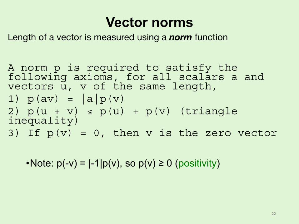
Vector normsLength of a vector is measured using a norm function

A norm p is required to satisfy the following axioms, for all scalars a and vectors u, v of the same length,1) p(av) = |a|p(v) 2) p(u + v) ≤ p(u) + p(v) (triangle inequality)3) If p(v) = 0, then v is the zero vector

There a variety of ways to measure length (i.e. multiple ways one can define a norm).

21

Vector norms

22

•Note: p(-v) = |-1|p(v), so p(v) ≥ 0 (positivity)

Length of a vector is measured using a norm function

A norm p is required to satisfy the following axioms, for all scalars a and vectors u, v of the same length,1) p(av) = |a|p(v) 2) p(u + v) ≤ p(u) + p(v) (triangle inequality)3) If p(v) = 0, then v is the zero vector

Norms of vectorsIf v is an m-by-1 column (or row) vector, the L2 “norm of v” is defined

as

23

Symbol to denote “norm of v”

Square-root of sum-of-squares of components, generalizing Pythagorean’s theorem

The norm of a vector is a measure of its length.

Helpful property:

||v + w|| ≤ ||v|| + ||w|| (Triangle inequality)

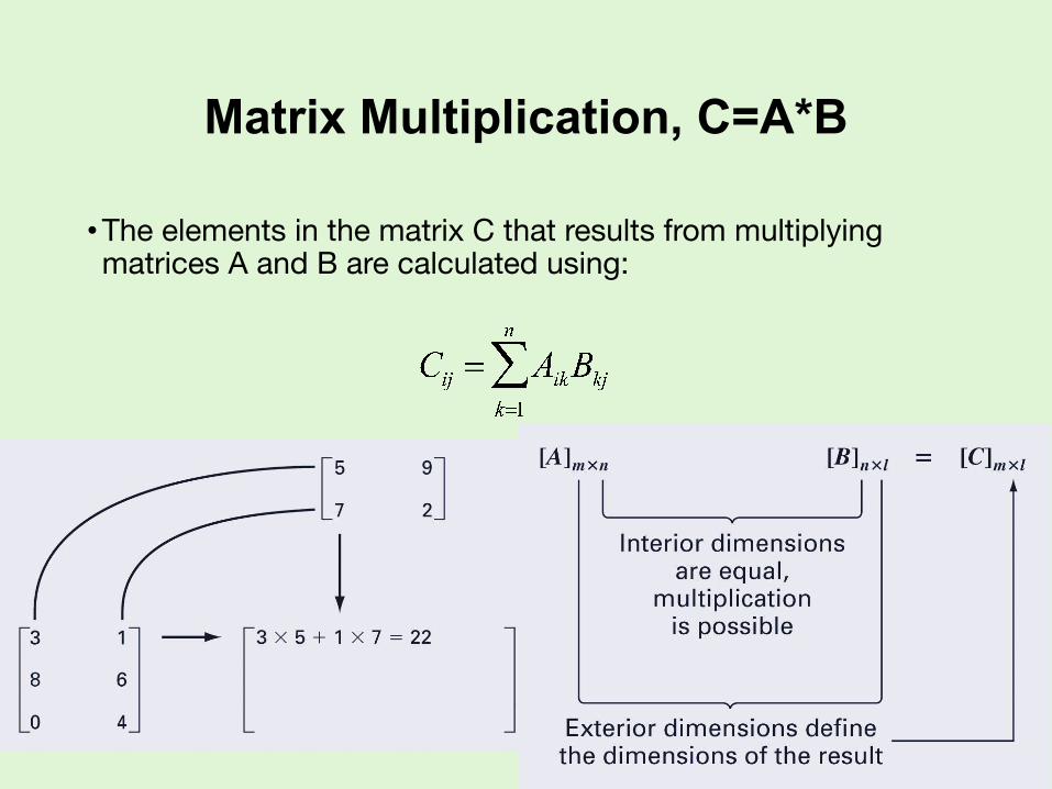
Matrix Multiplication, C=A*B

• The elements in the matrix C that results from multiplying matrices A and B are calculated using:

24

Matrix Math

•Does order of evaluation matter?• Is (A+B)+C = A+(B+C)?

25

Matrix Math

•Does order of evaluation matter?•Is (AB)C = A(BC)?

26

Matrix Math

•Does order of evaluation matter?•Is AB = BA?

27

Special Matrices••

28

What is a linear function?

29

Let be a function. It is said to be linear if

This is sometimes called superposition

Matrix representation of a linear function

30

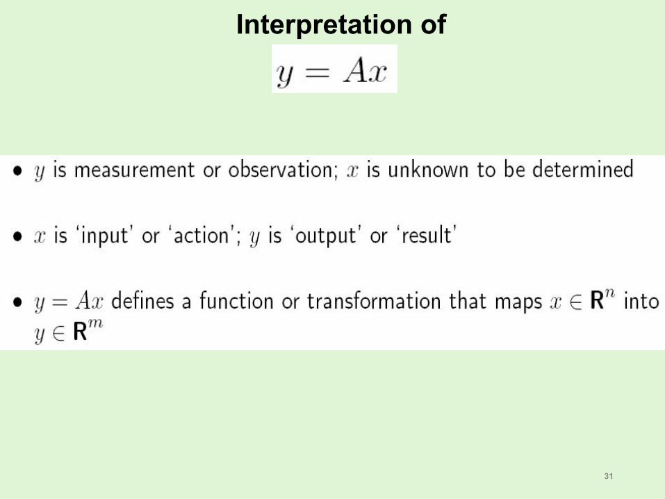
Interpretation of

31

Interpretation of in

32

Solving y=Ax

Graphing the equations can demonstratea) No solution existsb) Infinite solutions existc) System is ill-conditioned!!!

33

Linear equations

34

=

==

Square, equal number of unknowns and equations

Underdetermined: more unknowns than equations

Overdetermined: fewer unknowns than equations

Types of solutions with “random” data“Generally” the following observations would hold

35

=

==

One solution (eg., 2 lines intersect at one point)

Infinite solutions (eg., 2 planes intersect at many points)

No solutions (eg., 3 lines don’t intersect at a point)

Linear equations

36

=

==

No solution (2 parallel lines)Many solutions (2 identical lines)

No solutions (2 parallel planes)Solutions (3 lines that do intersect at a point)

Problem of inversion

37

For matrices, the definition of the “inverse”, or “one over” the matrix, has to be defined properly. When does the inverse exist?

In MATLAB, x = A\b Attempts to solve matrix equation Ax = b.

Use of \ is due to the fact matrix multiplications is not commutative, i.e.

AB = C => A\AB=A\C => B = A\C.

It is not the case B=C/A, i.e. AB/A is not B.

The Determinant

•Describes how volume defined by set of points X changes when when A is applied to X.

38

Determinants (square matrices)

39

Consider a 2 x 2 matrix

The determinant of a 2 x 2 matrix is

Finding the determinant of a general n x n square matrix requires evaluation of a complicated polynomial of the coefficients of the matrix, but there is a simple recursive approach. If the determinant is non-zero, the matrix can be inverted and unique solution exists for Ax=b. If the determinant is zero, the matrix cannot be inverted, there canbe either 0 or an infinite number of solutions to Ax=b.

Solving Ax=y

•When A is non-singular (has non-zero determinant) A inverse exists, and one can find x via

x = inv(A)*y

•However, depending on A, this is can be computationally inefficient and or less precise then using x = A\y

•The MATLAB \ operation (called mldivide) takes the form of A into account while trying to solve A\y

•doc mldivide

40

Operation of A\y in MATLAB

41

42

43

Solving Ax=y

•When A is singular (has a zero determinant) A inverse does not exist

• In this case there are either NO solutions or there are an INFINITE number of solutions to Ax = b

•Two key questions1) How can we tell when no solutions exist?2) When solutions exists how can we find and represent them?

https://www.mathworks.com/help/matlab/math/systems-of-linear-equations.html

44



HW Problem 7.1.7

•For an m-by-n array the linear index of element (i,j) is i+(j-1)*m

45

HW Problem 7.2.4

• Binary SearchSee next slides

46

Binary Search & BISECTION

47

Outline: Root Finding

• Key Concept: Search• Binary Search• Bisection Method

48

SearchingFinding a specific entry in a 1-dimensional (eg, column vector, row

vector) object.

Brute force approach, scan (potentially) the entire list.

function Idx = bfsearch(A,Key)N = length(A);Idx=1;while Idx<=N & A(Idx)~=Key Idx = Idx + 1;endif Idx==N+1 Idx = []; % no match foundend

49

Loop exits ifIdx>N orA(Idx)==Key

Match found

Entire list scanned, no match found

Searching in a sorted list

••“ ” “ ”

•

50

Match must be over here


“ ”

51



Searching in a sorted list

Simple Binary Search ExampleLet’s do an example with as below, and Key = 0.1; A

52

L = 1;R = length(A);while R>L M = floor((L+R)/2); if A(M)<Key L = M+1; else R = M; endend

Motivation for Root Finding: Solving Equations

From linearity, it is easy to solve the equation

or even the system of equations

But what about an equation like

53

From linearity, it is easy to solve the equation

or even the system of equations

But what about an equation like

54

Finding Roots

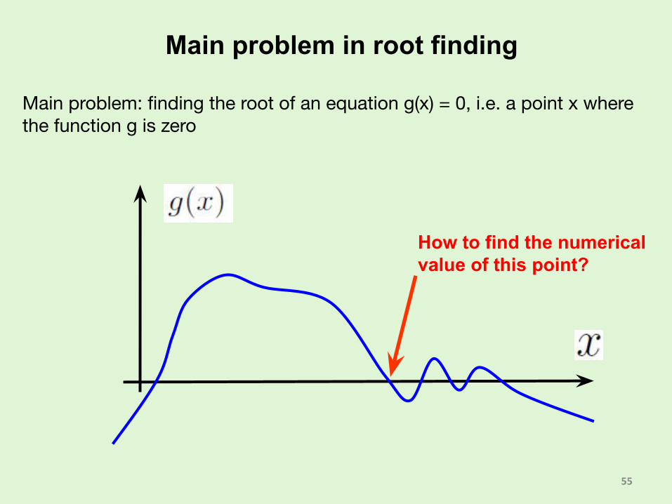
Main problem in root finding

Main problem: finding the root of an equation g(x) = 0, i.e. a point x where the function g is zero

How to find the numerical value of this point?

Matlab built in functions

Matlab has a generic function called fzero which finds a zero of a function, based on a guess entered by a user.

Declare function using function handle

Call fzero, and specify guess

Result is obviously π/2 in this case, as can be checked

What questions are involved in solving g(x)=0?

Root finding algorithms find numerical values such that the function g is “almost” zero, i.e. has small values.

In this band, the function is “small enough” that it can be considered to be almost equal to zero

What questions are involved in solving f(x)=0?


What does this mean numerically?

Let us zoom and see what is happening here.



As long as the function is in the pink strip, we consider it equal to zero, thus any point in the corresponding horizontal segment is an approximation of the root


This can be a problem if the function is too “flat”

This function is too flat, thus, a better criterion would be “vertical” (not horizontal)

What questions are involved in solving g(x)=0?

This can be a problem if the function is too “flat”

If one could say that the root is in this vertical slab, it would be more meaningful

How do root finding algorithms work?

In general root finding algorithms have three features1) A guess or initialization procedure2) An iterative procedure to refine the approximation of the solution3) A stopping criterion (when the solution is “good enough”)

Start: input guess of the problem (or initialize the problem)

While (solution not good enough)Refine the solution

Stop: when solution is good enough

MathematicallyIterative methods start with a “guess”, labeled x0 and through “easy” calculations, generate a sequence

x1, x2, x3, …

Goal is that sequence satisfies

and

63

convergence to a limit, x*

x* is a solution

One useful theorem for root finding

Theorem (Intermediate Value):

If g is a real-valued continuous function on the interval [a, b], and u is a number between g(a) and g(b), then there is a c ∈ [a, b] such that g(c) = u.

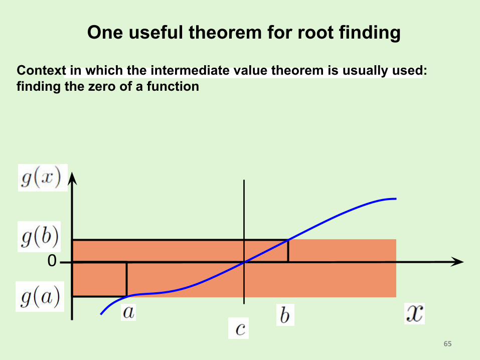
One useful theorem for root finding

Context in which the intermediate value theorem is usually used: finding the zero of a function

Bisection algorithm

Initialization step: enter a and b, such that g(a) and g(b) are of opposite signs, thus the function has at least one zero between a and b. Whenever this is true g(a)g(b) is negative.

INITIALIZATION STEP

Bisection algorithm

Refinement step: compute midpoint m = (a+b)/2, and evaluate the sign of g(a)g(m)

REFINEMENT STEP

Analyze the situation: g(a)g(m) positive => g(a) and g(m) have the same sign, so the root must be between m and b

REFINEMENT STEP

Root is in this interval

Bisection algorithm

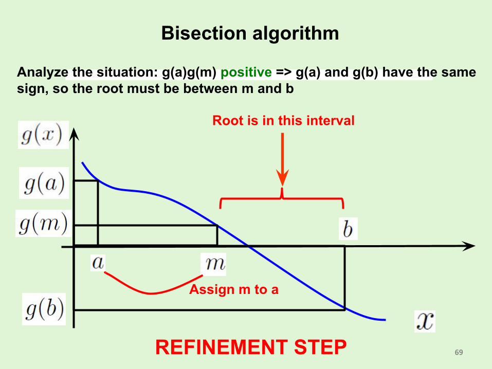
Analyze the situation: g(a)g(m) positive => g(a) and g(b) have the same sign, so the root must be between m and b

REFINEMENT STEP

Root is in this interval

Assign m to a

Bisection algorithm

Now we have a new interval and we can start the search again

REFINEMENT STEP

This becomes the new interval [a,b]

Bisection algorithm

Compute the new midpoint for the new interval (as in the previous step)

REFINEMENT STEP

Compute the new midpoint for this inteval [a,b]

Bisection algorithm

Evaluate the sign of g(a)g(m), here g(a)g(m) is negative

REFINEMENT STEP

There is a root between a and m.

Bisection algorithm

Evaluate the sign of g(a)g(m), here g(a)g(m) is negative

REFINEMENT STEP

When g(a)g(m) is negative, assign m to b

Bisection algorithm

Evaluate the sign of the function at the midpoint

REFINEMENT STEP

Now use this interval for the next iteration

Bisection algorithm

Evaluate the sign of the function at the midpoint

STOPPING CRITERION

Stop when one of the criteria is satisfied.

Bisection algorithm

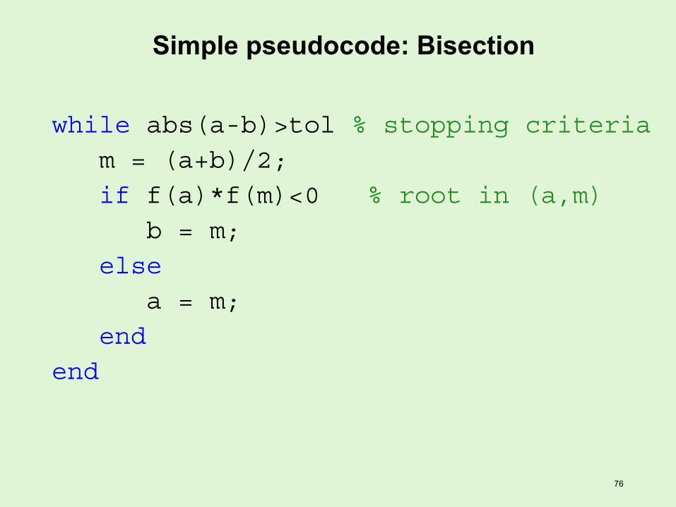
while abs(a-b)>tol % stopping criteria m = (a+b)/2; if f(a)*f(m)<0 % root in (a,m) b = m; else a = m; endend

76

Simple pseudocode: Bisection

•Always convergent•The root bracket gets halved with each iteration - guaranteed.

77

Advantages of Bisections

78

■ Slow convergence■ If one of the initial guesses is close to

the root, the convergence is slower

Drawbacks of Bisection

• If a function f(x) is such that it just touches the x-axis it will be unable to find the lower and upper guesses.

79


80

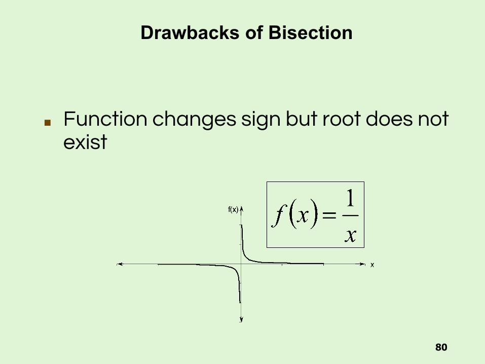
■ Function changes sign but root does not exist


HW Problem 7.3.5

•The MATLAB documentation on finding solutions to linear equations is very helpful


81



Documents

Lecture 17 Linear Algebra I - cs.brown.edu