Lecture 14 Tomography

P is direct P wave in mantlePcP is a reflection from the core Angle of incidence = Angle of reflection

Body wavesIn the interiorOf the Earth’s body

P arrives at about 7.7 minutes after the origin of the earthquakePcP arrives at 9.7 minutes

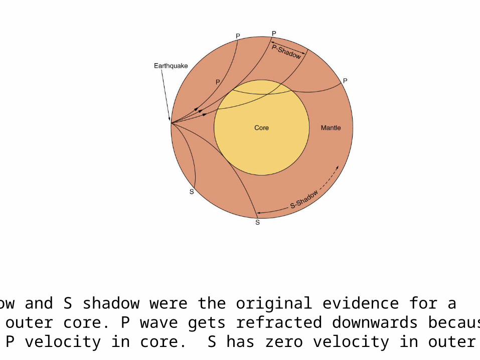
P shadow and S shadow were the original evidence for a liquid outer core. P wave gets refracted downwards becauseof low P velocity in core. S has zero velocity in outer core.

Tomography

Positron emission tomography (PET scan)

MRI (magnetic resonance imaging)

CAT Scan [computerized axial tomography (CAT) scan. A CT scanner directs a series of X-ray pulses through the body. ]

MRI 20 Tesla (Earth’s field 50000 nT

Travel time= distanc/velocity

Theoretical Tomography

The Radon transform is an integral transform whose inverse is used to reconstruct images from medical CT scans.

1( )

( , , )

velocity( , , ) Radon Transform( , )

T d pathvelocity x y z

x y z T path

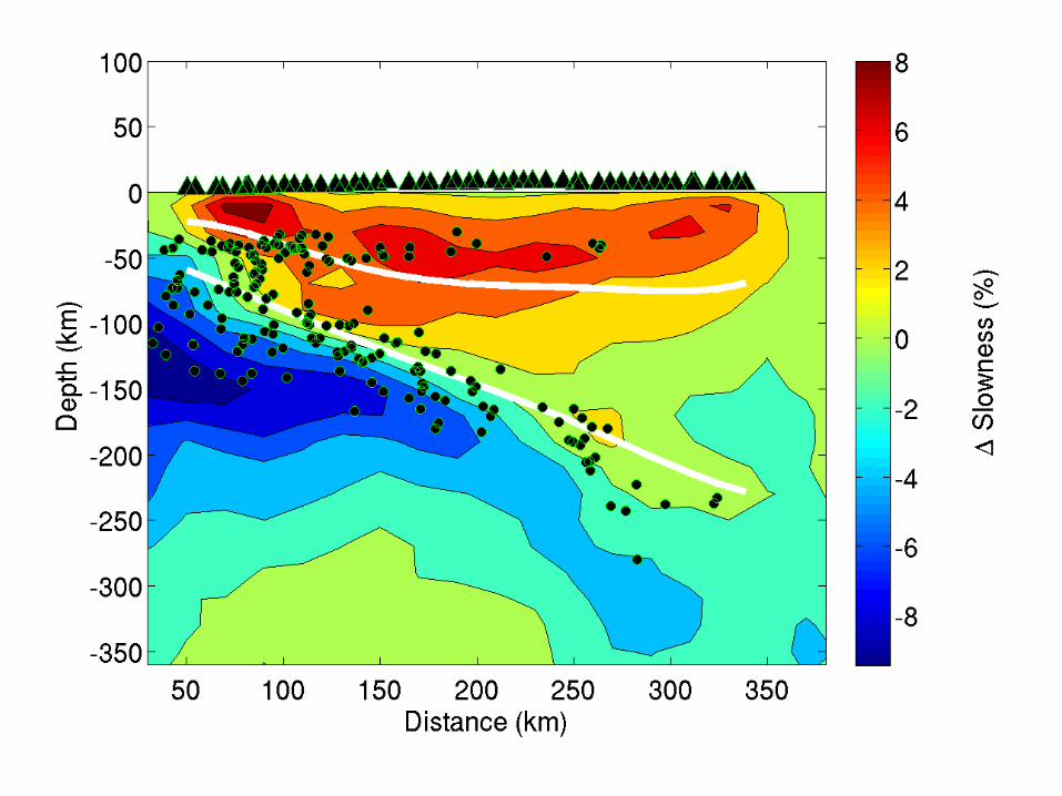
Seismic tomography uses earthquakes (or shots) to image lateralheterogeneity in the Earth’s interior.

Tomography beneath Yellowstone Caldera

Tomography shows shallow asthenospherebeneath Kenya dome on east African Rift

Tomography of the mantle and inner core.Note Africa and Pacific Super Plumes

(from John Woodhouse)

(from Adam Dziewonski)

Tomography

UCSD GlobalTomographic models

Slab graveyard 100-200 ma

Laboratory Experiments

• Lava Lamp• Shows plumes rising

Two deep plumes Two shallow plumes Montelli et al., Science 2004

Deep plumes

Shallow plumes

Plumes from Montelli et al., 2004

http://www.mala.bc.ca/~earles/mantle-plume-depths-jan04.htm

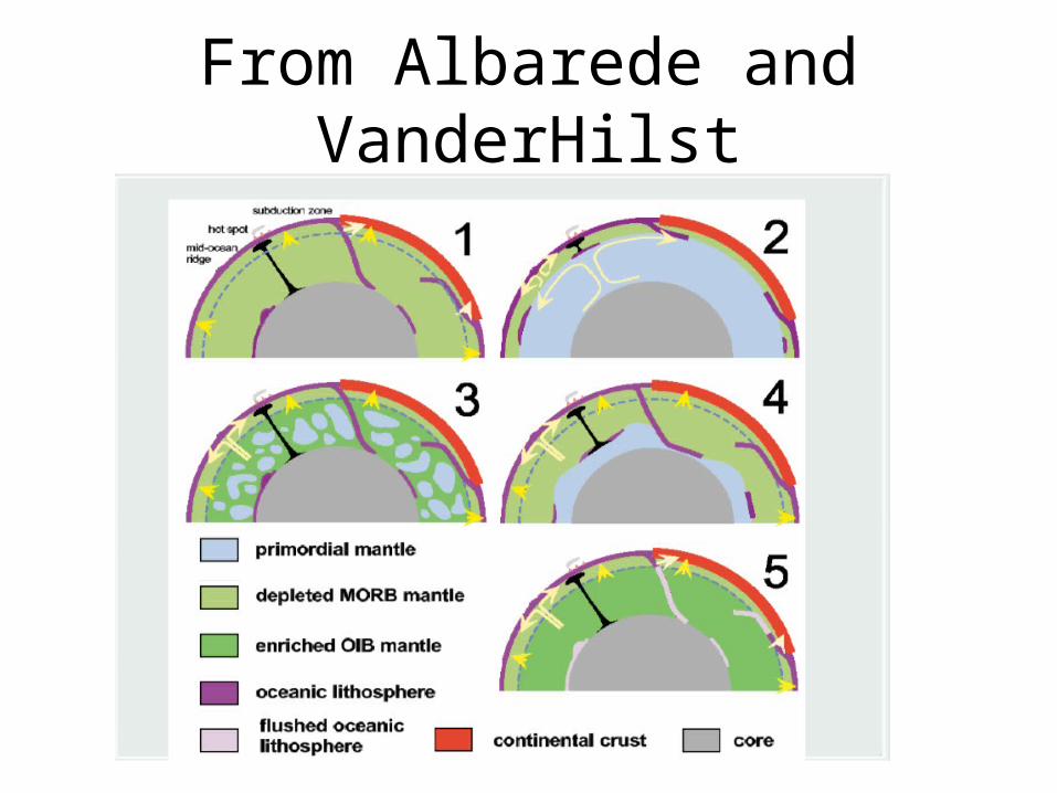
From Albarede and VanderHilst

Tomography of Furnace Creek Fault zone

Steps:1. Pick 48x48 arrivals using RAS24.exeSave as ascii2. Use linear velocity background modelV=a+bz analytic solutions for T, X3. Find average a b that fit data4. Find nearest node points on 5 m grid for rays5. Back project residuals along rays to form tomogram

Fit of background model

Rays One shotAnalytic for V=a+bz=1200+45z m/s

2 2 1/2 2 2 2 2 2 2 2 1/2x=(1-p b ) (pb)-(1-p b -2p b z-p b z ) /(pb);

1

% t= arctanh(--------------------------)

% 2 2 2 1/2

% (-p b (z + a/b) + 1)

% - -----------------------------------

% b

Shot at 12 th geophone 55 m.

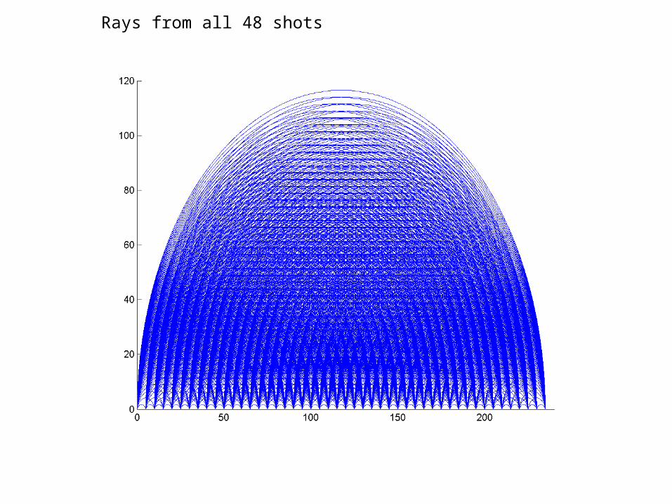
Rays from all 48 shots

Rays interpolated onto 48x48 5 meter grid

Hit count at each grid node

Tomogram

Tomogram after stacking travel times Note loader.m shows velocities

Axis (no vertical exaggeration) image view of tomogram

65m