Lecture 14: One distribution to rule them all.Part 1. Normal approximation to the binomial

distribution

CSCI2244-Randomness and Computation

April 9, 2019

1 Some picturesFigure 1 shows the PMFs of the random variables Sn,p for n = 40, 80, 100, andp = 0.5, 0.35, 0.5. where Sn,p denotes the number of heads on n tosses of a coinwith heads probability p. These PMFs are given by the binomial probability dis-tribution

P (Sn,p = k) =

(n

k

)pk(1− p)n−k.

The three random variables of course all have different expected values (20,28 and 50, respectively) so the PMFs are nonzero on different parts of the numberline. By our previous calculations, the standard deviation of Sn,p is

√np(1− p),

so these three random variables have standard deviations 3.16, 4.27 and 5, respec-tively.

While these are discrete distributions, you can imagine making a smooth curveby connecting the tops of the stems in each of the three plots. Since the stems inthis case are 1 unit apart, and the sum of the heights of the stems is 1, the areaunder each of the three imaginary curves is 1, and so they represent the graphs ofdensities.

We transform these random variables. In general, if X is a random variablewith mean E(X) = µ, and m is a constant, then X −m is a random variable withthe same variance as X, and with mean E(X−m) = E(X)−E(m) = µ−m. Inparticular, X − µ has mean 0. The effect on the graph of the PMF of X (or, in the

1

continuous case, the PDF) is to shift the graph a distance µ to the left. Otherwisethe graph is the same.

In Figure 2, Sn,p is transformed in this way to Sn,p − np, so that all threerandom variables have expected value 0.

Further, ifX is a random variable with standard deviation σ, , then the standarddeviation of the random variable X/s is σ/s. Thus if we start with X havingmean µ and standard deviation σ, then we can apply both these transformations insuccession and get a random variable (X−µ)

σwith mean 0 and standard deviation

1. The net effect is to shift by a distance of µ and to shrink horizontally by a factorof σ. Figure 3 shows the effect of these transformations, displaying the PMFs of

Sn,P − np√np(1− p)

.

In the last step, we destroyed the property that the area enclosed by each stemplot is 1: when we compressed the graph by a factor of σ, we divided this area byσ. To restore the property, we multiply the height of each graph by the standarddeviation σ =

√np(1− p). Figure 4 shows the remarkable result— all the points

appear to lie on the same smooth curve, which we have traced. What is this curve?It was drawn by plotting the graph of

φ(x) =1√2π· e−x2/2,

and the crucial result illustrated by these pictures is that this shape closely ap-proximates the binomial distribution. In other words, this famous ‘bell curve’represents a continuous probability density that is a kind of limiting case of thebinomial distributions as n grows large.

2 The normal distributionThe function φ is called the standard normal density. ‘Standard’ here means thatit has mean 0 and standard deviation 1. It’s not the least bit obvious that this is adensity: you would need to show that∫ ∞

−∞e−x

2/2dx =√

2π.

The proof of this is not hard, but it cannot be obtained by usual integration tech-niques, because there is no closed form expression for an antiderivative of e−x2/2.

2

Figure 1: PMFs of binomial distribution with n = 40, 80, 100 and p =0.5, 0.35, 0.5

3

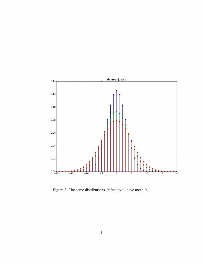
Figure 2: The same distributions shifted to all have mean 0...

4

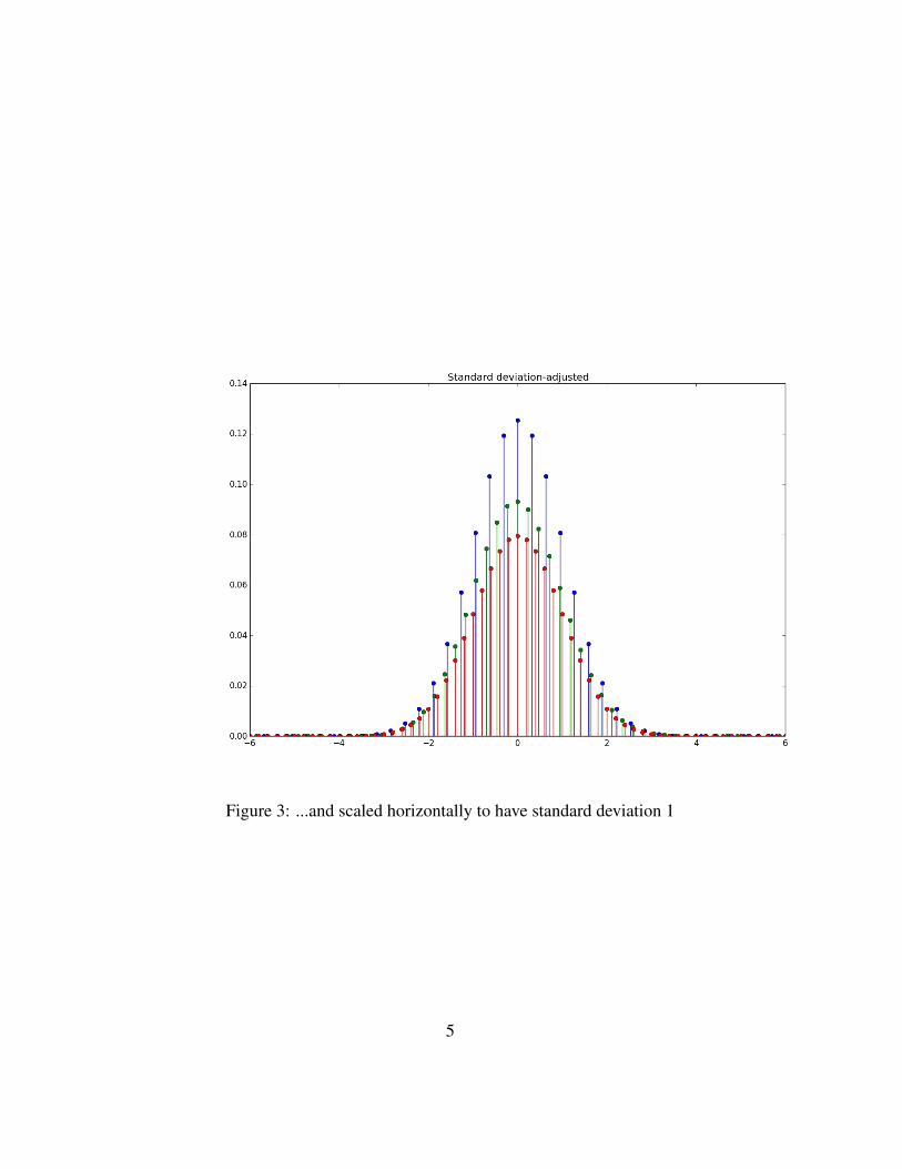
Figure 3: ...and scaled horizontally to have standard deviation 1

5

Figure 4: The previous figure stretched vertically by the standard deviation so thatall the total area under each graph is 1, superimposed on the graph of 1√

2πe−x

2/2.

6

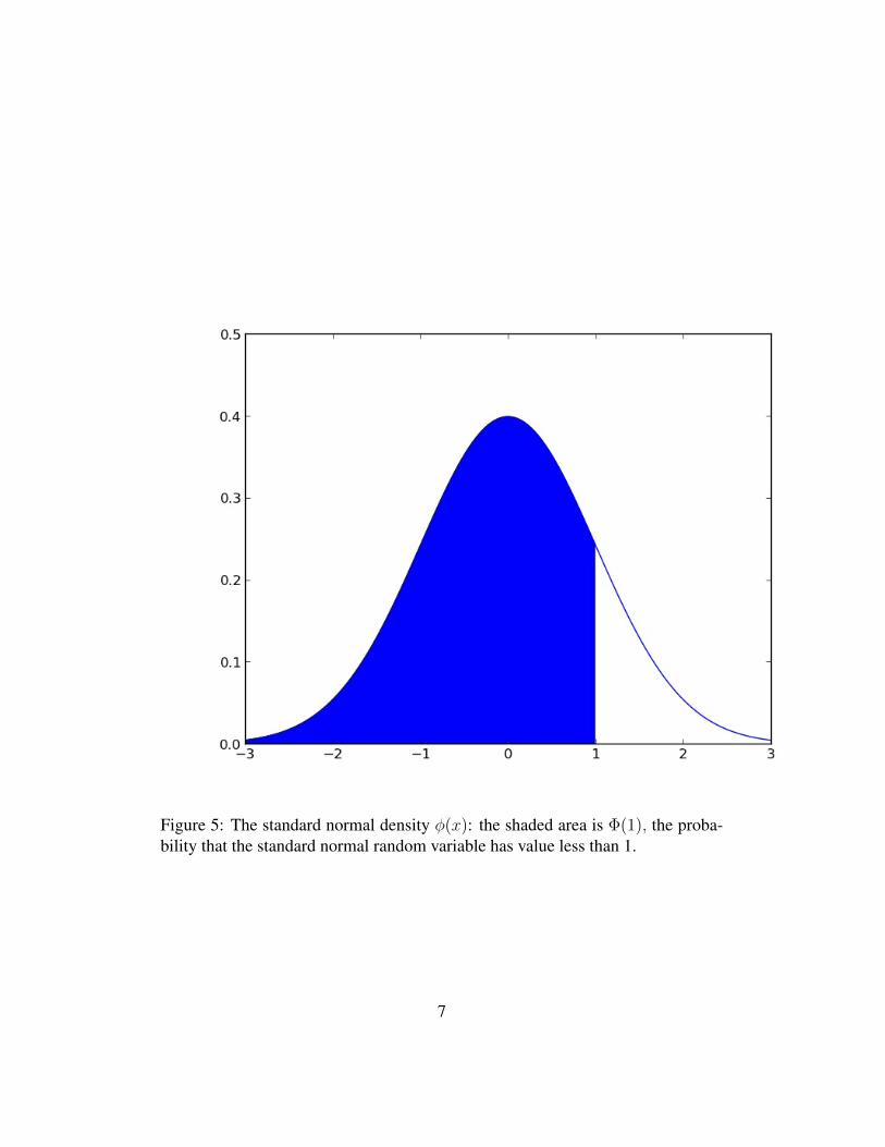
Figure 5: The standard normal density φ(x): the shaded area is Φ(1), the proba-bility that the standard normal random variable has value less than 1.

7

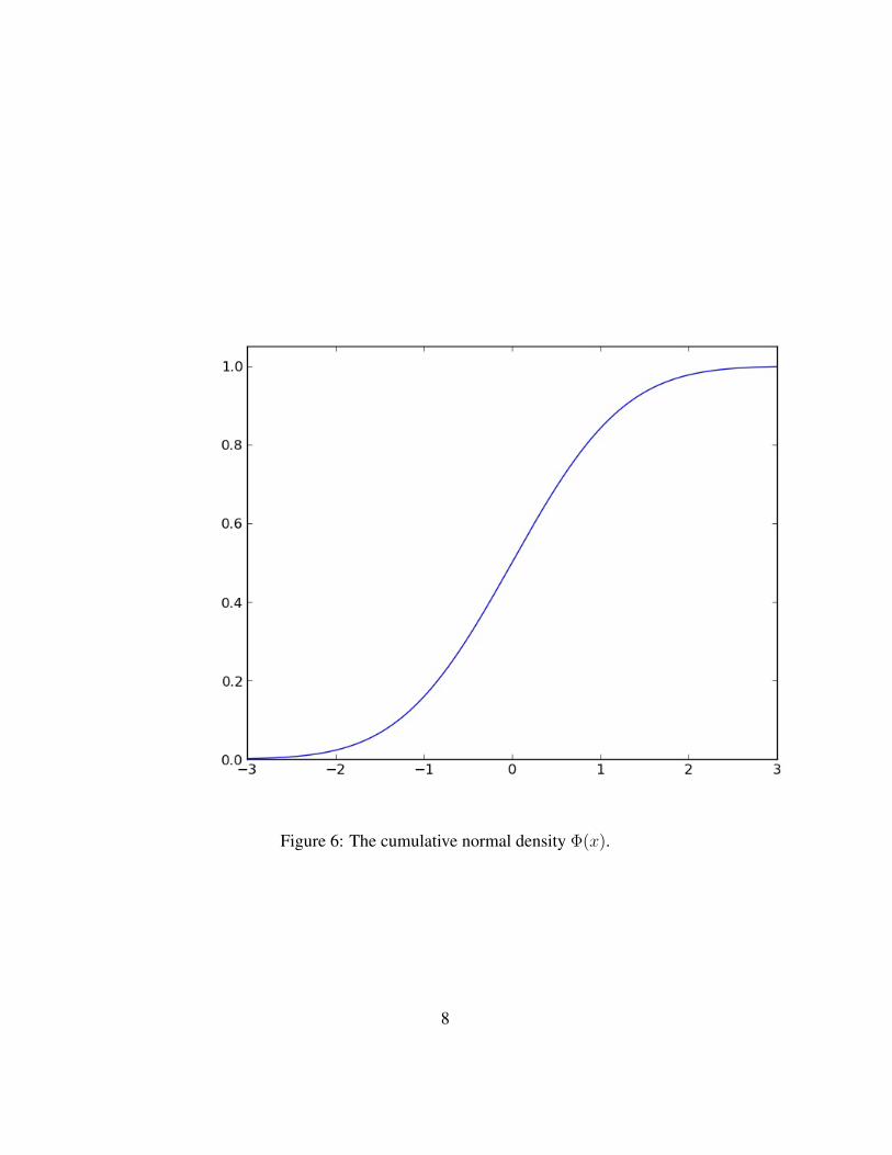
Figure 6: The cumulative normal density Φ(x).

8

The corresponding cumulative distribution function is

Φ(x) =1√2π

∫ x

−∞e−t

2/2dt.

Since we cannot evaluate Φ(x) analytically, it has to be approximated numerically.You can compute Φ(x) in Python with

from scipy.stats import normnorm.cdf(x)

You can similarly compute the inverse of the cumulative distribution functionwith norm.ppf.

If you drop the ‘standard’ part, there are infinitely many normal densities, onefor each choice of mean and standard deviation. The normal density with mean µand standard deviation σ is

1√2π · σ

e−x2/2σ2

.

3 Normal approximation to binomial distributionOur observations above illustrate an important fact: the binomial distribution, ad-justed to have mean 0 and standard deviation 1, is closely approximated by thenormal distribution, especially as n gets larger.

The general principle is that

P (a ≤ Sn,p − np√np(1− p)

≤ b) ≈ Φ(b)− Φ(a).

In the appendix (which is non-required reading) there is something like anexplanation of why this is true. Below we discuss what you can do with this fact.

Example. We use the normal approximation to the binomial distribution to esti-mate the probability that a fair coin tossed 100 times comes up heads between 45and 55 times, inclusive. That is, we want to evaluate

P (45 ≤ S100,0.5 ≤ 55).

Let us first note an issue. Since Sn,p is a discrete random variable that only takesinteger values, the probability above is identical to

P (44.5 ≤ S100,0.5 ≤ 55.5)

9

and evenP (44 < S100,0.5 < 56),

but these will give us three different answers if we use them as the basis for calcu-lating the normal approximation. It turns out that we get the best results by goingexactly halfway between the integer values. We then have

P (44.5 ≤ S100,0.5 ≤ 55.5) = P (44.5− 50√100× 0.25

≤ S100,p − 50√100× 0.25

≤ 55.5− 50√100× 0.25

)

= P (−1.1 ≤ S100,p − 50√100× 0.25

≤ 1.1)

≈ Φ(1.1)− Φ(−1.1)

= 0.728668.

Because of the symmetry in the event, we could have also evaluated this as

1− 2 · Φ(−1.1).

For purposes of comparison, we actually can compute the exact value in this case.It is

2−10055∑j=45

(100

j

)≈ 0.728747,

so our approximation is accurate to four decimal digits. Incidentally, had we used45 and 55 as the initial bounds, we would have gotten the approximation

Φ(1)− Φ(−1) = 0.682689,

which gives only one decimal digit of accuracy!If we wanted to know the probability that we get more than 55 heads, we can

use the result of the above calculation, subtracting from 1 and dividing by 2. (Or,what is the same thing, taking Φ(−1.1).) The result is 0.13566.

Let us ask more generally, what is the probability of getting between 45%and 55% heads on N tosses of the coin, for large N? If we repeat the abovecalculation, the lower limit -1.1 in the approximation gets replaced by

(0.45N − 1

2N−N/2)/(

√(N)/2)

10

so the probability is approximately

1− 2Φ(−0.1√N − 1

N√N

).

Since −0.1√N − 1

N√N

tends to −∞ as N gets large, the probability approaches1. We already knew this, thanks to the law of large numbers, but now we canestimate it very accurately. For example, with N = 1000 we get 0.9986, whichagrees with the exact answer to 4 decimal places.

Example. This example concerns election polling. A large number N of peoplehave voted in an election in which there are two candidates, A and B. We sampleS voters and determine the number k of these S voters who voted for A. The value

p̄ = k/S

serves as the estimate of the proportion p of voters in the entire population whovoted for A.

How large should we make S? Let’s say we have a target accuracy—we wouldlike our estimate to be within 3% of the actual vote, so that if, say, 54% of the totalpopulation voted for A, then p̄would be between 0.51 and 0.57. That is, we wouldlike to be sure that

|p̄− p| ≤ 0.03.

Of course, there is no way we can be absolutely sure of this without samplingalmost all the voters in the population. Instead, noting that p̄ is a random variable,we will try to choose k such that

P (|p̄− p| ≤ 0.03) ≥ 0.95.

The threshold 95% is frequently used in such calculations. This is referred to asthe confidence level, and 3% as the margin of error.

Since the sampling is done without replacement, k has a hypergeometric dis-tribution, which depends on both N and S. But, as we’ve observed before, sinceN is very large, k is for all practical purposes a binomial random variable thatdepends only on S and p. Thus

k − Sp√Sp(1− p)

11

is well approximated by a standard normal random variable. We have

k − Sp√Sp(1− p)

=S√

Sp(1− p)·(k

S− p)

=

√S

p(1− p)· (p̄− p).

So this last expression is a random variable with approximately the standardnormal distribution. We thus have

P (|p̄− p| ≤ 0.03) = P (−0.03 ≤ p̄− p ≤ 0.03)

= P

(−0.03

√S

p(1− p)≤

√S

p(1− p)· (p̄− p) ≤ 0.03

√S

p(1− p)

)

≈ Φ

(0.03

√S

p(1− p)

)− Φ

(−0.03

√S

p(1− p)

)

= 1− 2Φ

(−0.03

√S

p(1− p)

).

Thus we need to solve

1− 2Φ

(−0.03

√S

p(1− p)

)≥ 0.95,

that is,

Φ

(−0.03

√S

p(1− p)

)≤ 0.025.

We can could use the inverse normal cdf for this. This result is

0.03

√S

p(1− p)≈ 1.96.

The usual practice is to call this 2, and to treat±2 standard deviations as the ‘95%confidence interval’. In fact this gives 95.4% confidence.

So now we need to solve

0.03

√S

p(1− p)≥ 2.

12

We don’t know what p is, but if 0 ≤ p ≤ 1, then p(1−p) ≤ 14. Thus it is sufficient

to solve0.03√

4S ≥ 2,

which gives S ≈ 1111. So say, candidate A receives 54% of the total vote and youpoll 1200 voters. Approximately 95% of the time you perform this experiment,you will find that between 51% and 57% of the voters in your sample voted forcandidate A.

4 Nonrequired reading for the mathematically curi-ous: The standard normal density really is a den-sity and it really is standard

While we don’t have a simple closed formula for the integral of e−x2 , we cannonetheless evaluate the improper integral

I =

∫ ∞−∞

e−x2

dx.

We’ll sneak up on the answer by finding the volume under the surface obtainedwhen you rotate the graph of e−x2 about the y-axis. The shape is shown below. In(x, y, z)-coordinates, the surface is the graph of the equation

z = e−(x2+y2).

There are two different approaches for computing this volume: We can takecross sections for each fixed value of x and add up (that is, integrate over) theareas of all these cross sections. Let’s call the area of the cross section Cx. Thenthe volume is

V =

∫ ∞−∞

Cxdx.

Now the cross section is just the graph of e−(x2+y2) where x is fixed and y varies,so its area is

Cx =

∫ ∞−∞

e−(x2+y2)dy = e−x

2

∫ ∞−∞

e−y2

dy = e−x2 · I.

ThusV = I ·

∫ ∞−∞

e−x2

dx = I2.

13

Figure 7: What you get when you rotate the graph of e−x2 about the vertical axis.

14

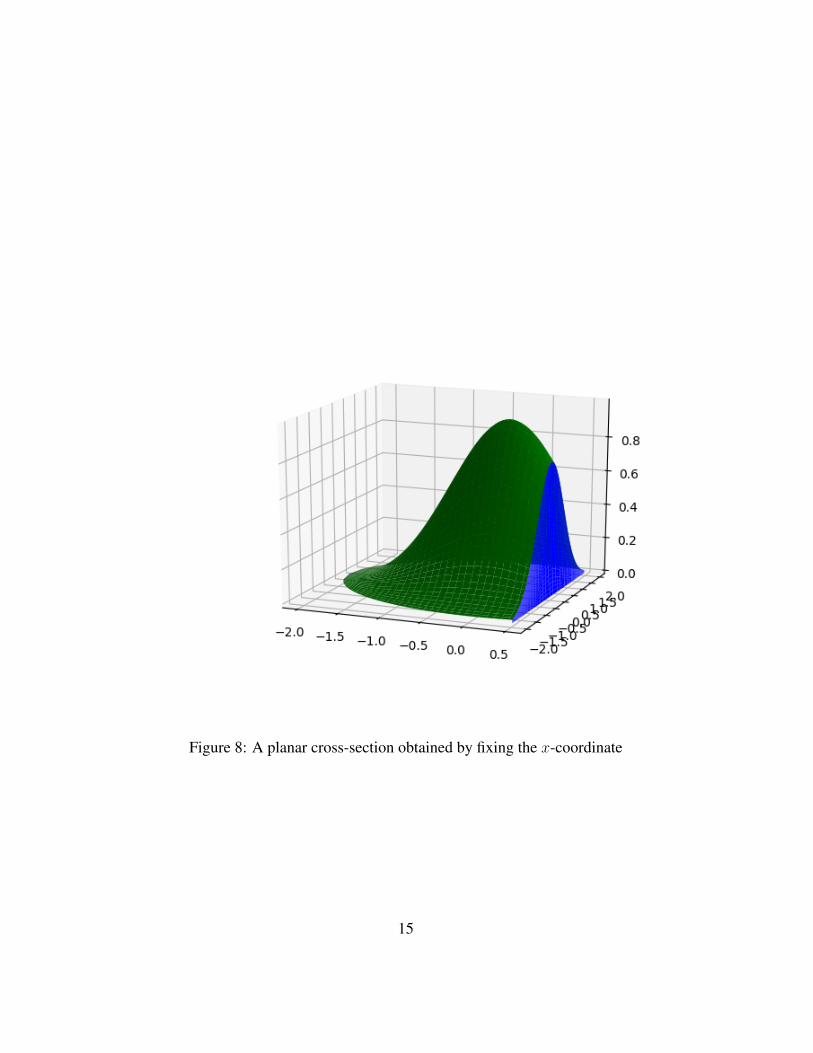
Figure 8: A planar cross-section obtained by fixing the x-coordinate

15

Figure 9: A cylindrical cross-section obtained by fixing the radius of rotation

16

The other way to obtain the volume is to integrate over the lateral areas of allthe cylindrical cross-sections you get by fixing the distance r > 0 from the originin the (x, y)-plane–this is a technique for finding the volumes of solids of rotationthat you may have learned in calculus. The area Cr of the cylinder is 2πre−r

2 andthus

V =

∫ ∞0

2πre−r2

dr

= −π · e−r2∣∣∣∣∞0

= −π · (0− 1)

= π.

So I2 = π and thus I =√π.

We find ∫ ∞−∞

e−x2/2dx =

√2π

by making a change of variables u = x√2

and applying the above result. Thus

1√2πe

−x2

2

integrates to 1: The standard normal density really is a density.What is the variance? Since E(X) = 0, the variance is just

E(X2) =1√2π

∫ ∞−∞

x2e−x2

2 dx.

We integrate by parts, setting u = x, dv = xe−x2

2 dx, so du = dx, v = −e−x2

2 .The formula for integration by parts gives

1√2π·(xe

−x2

2

∣∣∣∣∞−∞

+

∫ ∞−∞

e−x2

2 dx

)=

1√2π

(0 +√

2π) = 1.

So the standard normal density really is ‘standard’, in the sense that its stan-dard deviation is 1.

17