Nikolova 2020 1

LECTURE 14: LINEAR ARRAY THEORY - PART II

(Linear arrays: Hansen-Woodyard end-fire array, directivity of a linear array,

linear array pattern characteristics – recapitulation; 3-D characteristics of an

N-element linear array.)

1. Hansen-Woodyard End-fire Array (HWEFA)

The end-fire arrays (EFA) have relatively large HPBW as compared to

broadside arrays.

[Fig. 6-11, p. 270, Balanis]

Nikolova 2020 2

To enhance the directivity of an end-fire array, Hansen and Woodyard

proposed that the phase shift of an ordinary EFA

kd = (14.1)

be increased as

2.94

kdN

= − +

for a maximum at 0 = , (14.2)

2.94

kdN

= + +

for a maximum at 180 = . (14.3)

Conditions (14.2)–(14.3) are known as the Hansen–Woodyard conditions for

end-fire radiation. They follow from a procedure for maximizing the directivity,

which we outline below.

The normalized pattern AFn of a uniform linear array is

( )

( )

sin cos2

cos2

n

Nkd

AFN

kd

+

+

(14.4)

if coskd = + is sufficiently small (see previous lecture). We are looking

for an optimal , which results in maximum directivity. Let

pd = − , (14.5)

where d is the array spacing and p is the optimization parameter. Then,

( )

( )

sin cos2

cos2

n

Ndk p

AFNd

k p

−

=

−

.

For brevity, use the notation / 2Nd q= . Then,

sin ( cos )

( cos )n

q k pAF

q k p

−=

−, (14.6)

or sin

n

ZAF

Z= , where ( cos )Z q k p= − .

Nikolova 2020 3

The radiation intensity becomes

22

2

sin( ) n

ZU AF

Z = = , (14.7)

2sin ( )

( 0)( )

q k pU

q k p

−= =

− , (14.8)

2( ) sin

( )( 0) sin

n

U z ZU

U z Z

= =

= , (14.9)

where

( )z q k p= − ,

( cos )Z q k p= − , and

( )nU is normalized power pattern with respect to 0 = .

The directivity at 0 = is

0

4 ( 0)

rad

UD

P

== (14.10)

where ( )rad nP U d

= . To maximize the directivity, 0 / 4radU P = is

minimized.

22

0

0 0

1 sinsin

4 sin

z ZU d d

z Z

=

, (14.11)

22

0

0

sin ( cos )1sin

2 sin ( cos )

q k pzU d

z q k p

− =

− , (14.12)

2

0

1 cos2 1 1Si(2 ) ( )

2 sin 2 2 2

z zU z g z

kq z z kq

− = + + =

. (14.13)

Here, ( )0

Si (sin / )z

z t t dt= . The minimum of ( )g z occurs when

( ) 1.47z q k p= − − , (14.14)

Nikolova 2020 4

( ) 1.472

Ndk p − − .

1.47, where2 2

Ndk Ndpdp − − = −

( ) 1.472

Ndk + −

2.94 2.94

kd kdN N

− − = − +

. (14.15)

Equation (14.15) gives the Hansen-Woodyard condition for improved directivity

along 0 = . Similarly, for 180 = ,

2.94

kdN

= + +

. (14.16)

Usually, conditions (14.15) and (14.16) are approximated by

kdN

+

, (14.17)

which is easier to remember and gives almost identical results since the curve

( )g z at its minimum is fairly flat.

Conditions (14.15)-(14.16), or (14.17), ensure maximum directivity in the

end-fire direction. There is, however, a trade-off in the side-lobe level, which is

higher than that of the ordinary EFA. Besides, conditions (14.15)-(14.16) have

to be complemented by additional requirements, which would ensure low level

of the radiation in the direction opposite to the main lobe.

(a) Maximum at 0 = [reminder: coskd = + ]

0

0180

2.94

2.94

2.942 .

Nkd

Nkd

N

=

= =

= −

= − +

= − −

(14.18)

Since we want to have a minimum of the pattern in the 180 = direction, we

must ensure that

Nikolova 2020 5

180| | = . (14.19)

It is easier to remember the Hansen-Woodyard conditions for maximum

directivity in the 0 = direction as

0 180

2.94| | , | |

N N

= = = . (14.20)

(b) Maximum at 180 =

180

1800

2.94

2.94

2.942 .

Nkd

Nkd

N

=

= =

=

= +

= +

(14.21)

In order to have a minimum of the pattern in the 0 = direction, we must ensure

that

0| | = . (14.22)

We can now summarize the Hansen-Woodyard conditions for maximum

directivity in the 180 = direction as

180 0

2.94| | , | |

N N

= = = . (14.23)

If (14.19) and (14.22) are not observed, the radiation in the opposite of the

desired direction might even exceed the main beam level. It is easy to show (use

the relation 2 /kd N + ) that the complementary requirement | | = at the

opposite direction can be met if the following relation is observed:

1

4

Nd

N

−

. (14.24)

If N is large, / 4d . Thus, for a large uniform array, Hansen-Woodyard

condition can yield improved directivity only if the spacing between the array

elements is approximately / 4 .

Nikolova 2020 6

ARRAY FACTORS OF A 10-ELEMENT UNIFORM-AMPLITUDE HW EFA

Solid line: / 4d =

Dash line: / 2d =

N = 10

kdN

= − +

Fig. 6.12, p. 273, Balanis

Nikolova 2020 7

2. Directivity of a Linear Array

2.1. Directivity of a BSA

Using the approximate expression for the AF, the normalized radiation intensity

is obtained as

2

22

sin cossin2

( )

cos2

n

Nkd

ZU AF

N Zkd

= = =

(14.25)

0 0

0 4rad av

U UD

P U= = , (14.26)

where / (4 )av radU P = . The radiation intensity in the direction of maximum

radiation / 2 = in terms of nAF is unity:

0 max ( / 2) 1U U U = = = = ,

10 avD U − = . (14.27)

The radiation intensity averaged over all directions is calculated as

2

2 2

20 0 0

sin cos1 sin 1 2

sin sin4 2

cos2

av

Nkd

ZU d d d

NZkd

= = .

Change variable:

cos sin2 2

N NZ kd dZ kd d = = − . (14.28)

Then,

22

2

1 2 sin

2

Nkd

av

Nkd

ZU dZ

N kd Z

−

= −

, (14.29)

Nikolova 2020 8

22

2

1 sin

Nkd

av

Nkd

ZU dZ

Nkd Z−

=

. (14.30)

The function 1 2( sin )Z Z− is a relatively fast decaying function as Z increases.

That is why, for large arrays, where / 2Nkd is big enough ( )20 , the integral

(14.30) can be approximated by

21 sin

av

ZU dZ

Nkd Z Nkd

−

=

, (14.31)

0

12

av

Nkd dD N

U

= =

. (14.32)

Substituting the length of the array ( )1L N d= − in (14.32) yields

0 2 1

N

L dD

d

+

. (14.33)

For a large array ( )L d ,

0 2 /D L . (14.34)

2.2. Directivity of ordinary EFA

Consider an EFA with maximum radiation at 0 = °, i.e., kd = − .

( )

( )

2

22

sin cos 1sin2

( )

cos 12

n

Nkd

ZU AF

N Zkd

−

= = = −

, (14.35)

where (cos 1)2

NZ kd = − . The averaged radiation intensity is

2 22

0 0 0

1 sin 1 sinsin sin

4 4 2

radav

P Z ZU d d d

Z Z

= = =

.

Nikolova 2020 9

Since

(cos 1)2

NZ kd = − and sin

2

NdZ kd d = − , (14.36)

it follows that

2/2

0

1 2 sin

2

Nkd

av

ZU dZ

Nkd Z

−

= −

,

2/2

0

1 sinNkd

av

ZU dZ

Nkd Z

=

. (14.37)

If ( Nkd ) is sufficiently large, the above integral can be approximated as

2

0

1 sin 1

2av

ZU dZ

Nkd Z Nkd

= . (14.38)

The directivity then becomes

0

1 24

av

Nkd dD N

U

= =

. (14.39)

The comparison of (14.39) and (14.32) shows that the directivity of an EFA is

approximately twice as large as the directivity of the BSA.

Another (equivalent) expression can be derived for D0 of the EFA in terms of

the array length L = (N−1)d:

0 4 1L d

Dd

= +

. (14.40)

For large arrays, the following approximation holds:

0 4 / ifD L L d= . (14.41)

2.3. Directivity of HW EFA

If the radiation has its maximum at 0 = , then the minimum of avU is

obtained as in (14.13):

Nikolova 2020 10

2

min minminmin

min min

1 2 cos(2 ) 1Si(2 )

2 sin 2 2av

Z ZU Z

k Nd Z Z

− = + +

, (14.42)

where min 1.47 / 2Z = − − .

2

min1 2 0.878

1.85152 2

avUNkd Nkd

= + − =

. (14.43)

The directivity is then

0min

11.789 4

0.878av

Nkd dD N

U

= = =

. (14.44)

From (14.44), we can see that using the HW conditions leads to improvement of

the directivity of the EFA with a factor of 1.789. Equation (14.44) can be

expressed via the length L of the array as

0 1.789 4 1 1.789 4L d L

Dd

= + =

. (14.45)

Example: Given a linear uniform array of N isotropic elements (N = 10), find the

directivity 0D if:

a) 0 = (BSA)

b) kd = − (ordinary EFA)

c) /kd N = − − (Hansen-Woodyard EFA)

In all cases, / 4d = .

a) BSA

( )0 2 5 6.999 dBd

D N

=

b) Ordinary EFA

( )0 4 10 10 dBd

D N

=

Nikolova 2020 11

c) HW EFA

( )0 1.789 4 17.89 12.53 dBd

D N

=

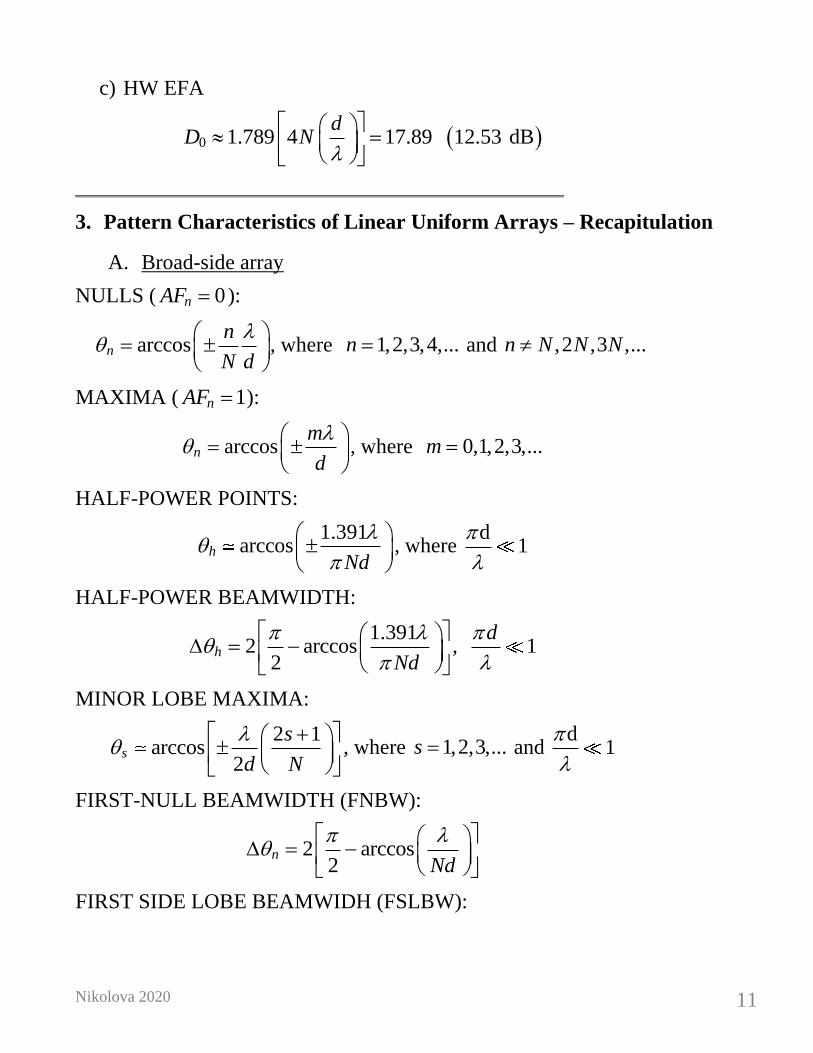
3. Pattern Characteristics of Linear Uniform Arrays – Recapitulation

A. Broad-side array

NULLS ( 0nAF = ):

arccosn

n

N d

=

, where 1,2,3,4,...n = and ,2 ,3 ,...n N N N

MAXIMA ( 1nAF = ):

arccosn

m

d

=

, where 0,1,2,3,...m =

HALF-POWER POINTS:

1.391

arccoshNd

, where d

1

HALF-POWER BEAMWIDTH:

1.391

2 arccos , 12

h

d

Nd

= −

MINOR LOBE MAXIMA:

2 1

arccos2

s

s

d N

+

, where 1,2,3,...s = and

d1

FIRST-NULL BEAMWIDTH (FNBW):

2 arccos2

nNd

= −

FIRST SIDE LOBE BEAMWIDH (FSLBW):

Nikolova 2020 12

3

2 arccos , 12 2

s

d

Nd

= −

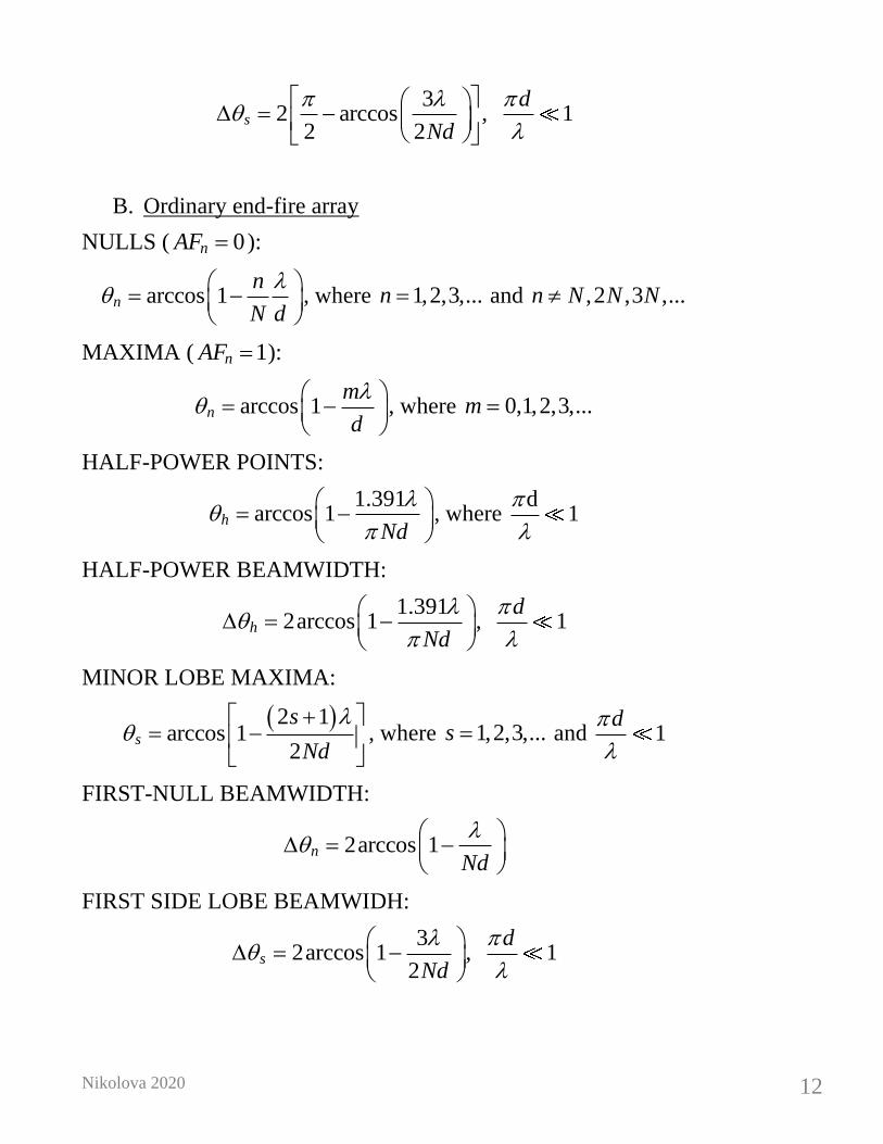
B. Ordinary end-fire array

NULLS ( 0nAF = ):

arccos 1n

n

N d

= −

, where 1,2,3,...n = and ,2 ,3 ,...n N N N

MAXIMA ( 1nAF = ):

arccos 1n

m

d

= −

, where 0,1,2,3,...m =

HALF-POWER POINTS:

1.391

arccos 1hNd

= −

, where

d1

HALF-POWER BEAMWIDTH:

1.391

2arccos 1 , 1h

d

Nd

= −

MINOR LOBE MAXIMA:

( )2 1

arccos 12

s

s

Nd

+ = −

, where 1,2,3,...s = and 1

d

FIRST-NULL BEAMWIDTH:

2arccos 1nNd

= −

FIRST SIDE LOBE BEAMWIDH:

3

2arccos 1 , 12

s

d

Nd

= −

Nikolova 2020 13

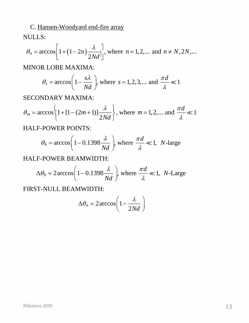
C. Hansen-Woodyard end-fire array

NULLS:

( )arccos 1 1 22

n nNd

= + −

, where 1,2,...n = and ,2 ,...n N N

MINOR LOBE MAXIMA:

arccos 1s

s

Nd

= −

, where 1,2,3,...s = and 1

d

SECONDARY MAXIMA:

arccos 1 [1 (2 1)]2

m mNd

= + − +

, where 1,2,...m = and 1

d

HALF-POWER POINTS:

arccos 1 0.1398hNd

= −

, where 1, -large

dN

HALF-POWER BEAMWIDTH:

2arccos 1 0.1398hNd

= −

, where 1, -Large

dN

FIRST-NULL BEAMWIDTH:

2arccos 12

nNd

= −

Nikolova 2020 14

4. 3-D Characteristics of a Linear Array

In the previous considerations, it was always assumed that the linear-array

elements are located along the z-axis, which is convenient to analyze in spherical

coordinate system. If the array axis has an arbitrary orientation, the array factor

can be expressed as

( )( ) ( )1 cos 1

1 1

N Nj n kd j n

n n

n n

AF a e a e − + −

= =

= = , (14.46)

where na is the excitation amplitude and coskd = + .

The angle is subtended by the array axis and the position vector to the

observation point. Thus, if the array axis is along the unit vector a ,

ˆ ˆ ˆ ˆsin cos sin sin cosa a a a a = + +a x y z (14.47)

and the position vector to the observation point is

ˆ ˆ ˆ ˆsin cos sin sin cos = + +r x y z (14.48)

the angle can be found as

ˆ ˆcos sin cos sin cos sin sin sin sin cos cos ,a a a a a = = + +a r

cos sin sin cos( ) cos cosa a a = − + . (14.49)

If ˆ ˆ ( 0 )a= = a z , then cos cos , = = .