Lecture 14: Deep Generative Learning Generative ...cvlab.postech.ac.kr/~bhhan/class/cse703r_2016s/... · Variational Autoencoder • Characteristics § A Bayesian approach on an autoencoder:

Lecture14:DeepGenerativeLearning

Bohyung [email protected]

CSED703R:DeepLearningforVisualRecognition(2016S)

GenerativeModelingbyNeuralNetworks

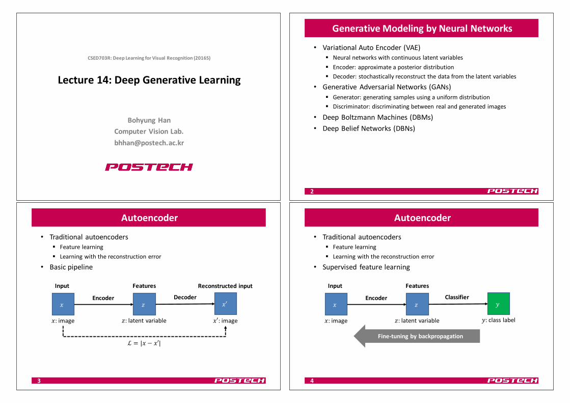
• Variational AutoEncoder(VAE)§ Neuralnetworkswithcontinuouslatentvariables§ Encoder:approximateaposteriordistribution§ Decoder:stochasticallyreconstructthedatafromthelatentvariables

• GenerativeAdversarialNetworks(GANs)§ Generator:generatingsamplesusingauniformdistribution§ Discriminator:discriminatingbetweenrealandgeneratedimages

• DeepBoltzmannMachines(DBMs)• DeepBeliefNetworks(DBNs)

2

Autoencoder

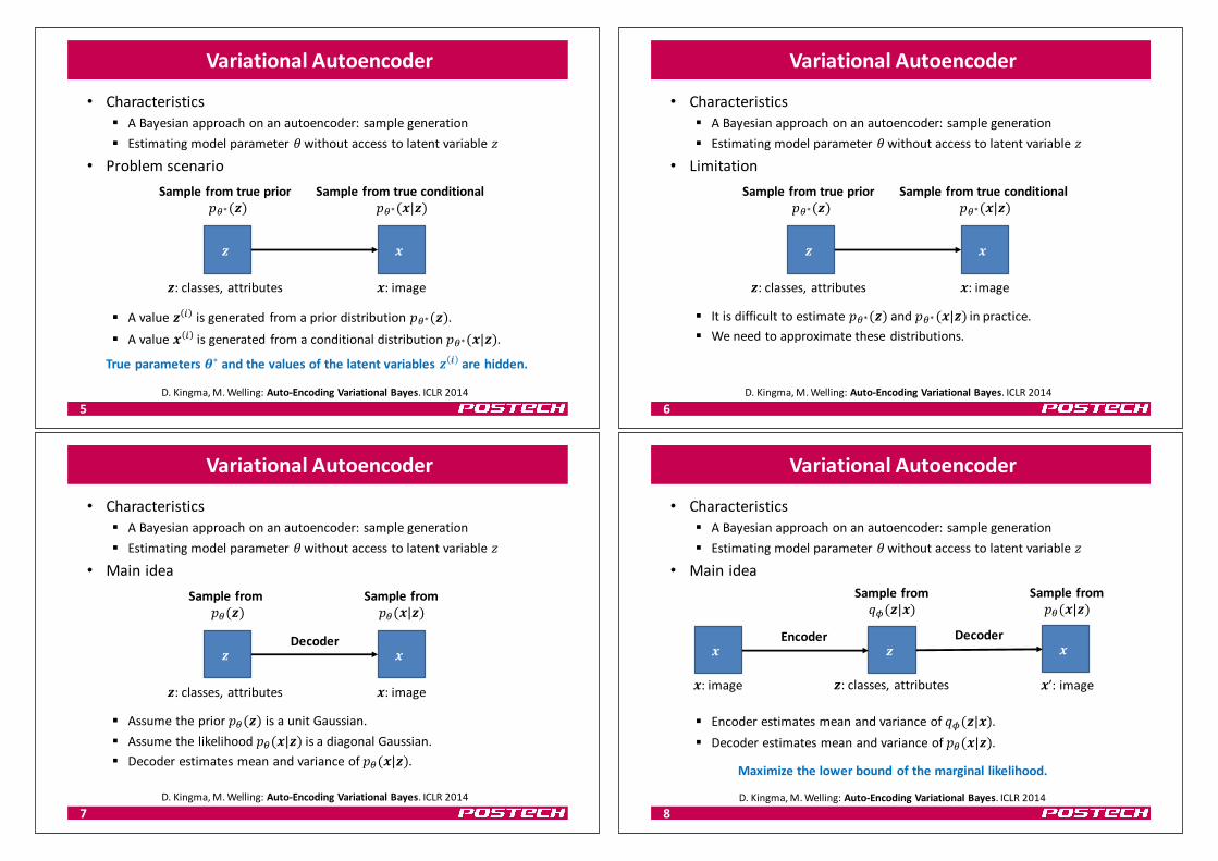
• Traditionalautoencoders§ Featurelearning§ Learningwiththereconstructionerror

• Basicpipeline

3

! "

Features

!: image ":latentvariable

Encoder!′

Decoder

Reconstructedinput

!′: image

Input

ℒ = ! − !′

Autoencoder

• Traditionalautoencoders§ Featurelearning§ Learningwiththereconstructionerror

• Supervised featurelearning

4

! "

Features

!: image

Encoder'

Classifier

':classlabel

Input

Fine-tuningbybackpropagation

":latentvariable

Variational Autoencoder

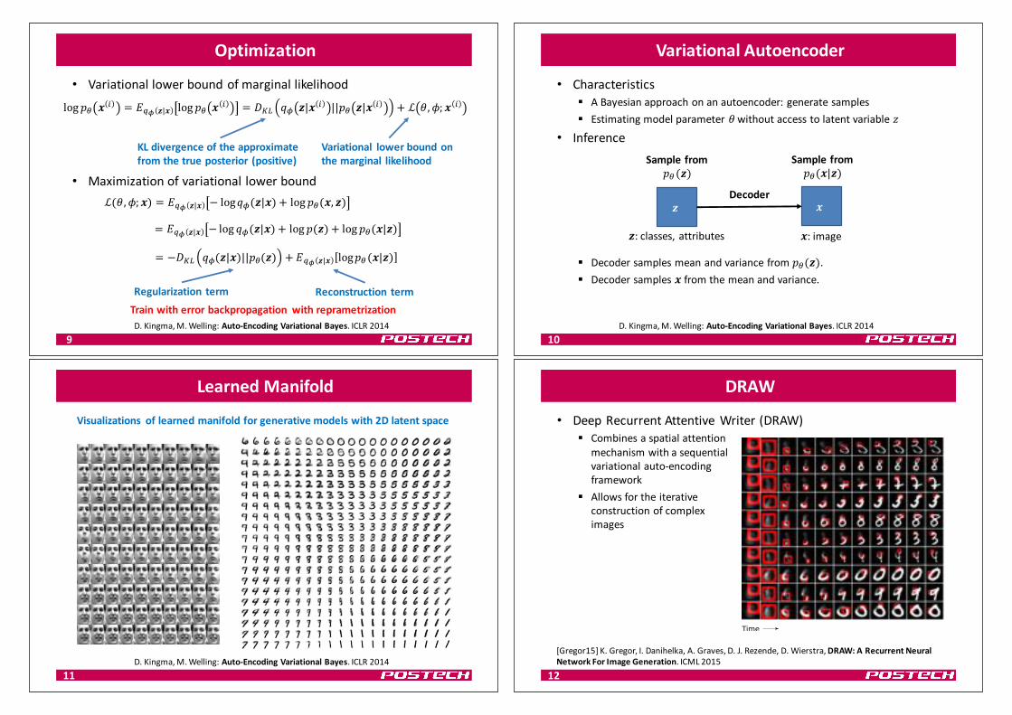
• Characteristics§ ABayesianapproachonanautoencoder:sample generation§ Estimatingmodelparameter(withoutaccesstolatentvariable"

• Problemscenario

§ Avalue) * isgenerated fromapriordistribution+,∗()).§ Avalue0 * isgenerated fromaconditionaldistribution+,∗(0|)).

5

) 0

Samplefromtrueprior+,∗())

Samplefromtrueconditional+,∗(0|))

0: image):classes,attributes

Trueparameters2∗ andthevaluesofthelatentvariables) 3 arehidden.

D.Kingma,M.Welling:Auto-EncodingVariational Bayes. ICLR2014



• Limitation

§ Itisdifficulttoestimate+,∗()) and+,∗ (0|)) inpractice.§ Weneedtoapproximatethesedistributions.

6

) 0

Samplefromtrueprior+,∗())

Samplefromtrueconditional+,∗(0|))





• Mainidea

§ Assumetheprior+,()) isaunitGaussian.§ Assumethelikelihood+,(0|)) isadiagonalGaussian.§ Decoderestimatesmeanandvarianceof+,(0|)).

7

) 0

Samplefrom+,())

Samplefrom+,(0|))


Decoder




• Mainidea

§ Encoderestimatesmeanandvarianceof45()|0).§ Decoderestimatesmeanandvarianceof+,(0|)).

8

0 )

Samplefrom45()|0)

0: image ):classes,attributes

Encoder0

Decoder

Samplefrom+,(0|))

0’: image

Maximizethelowerboundofthemarginallikelihood.


Optimization

• Variational lowerboundofmarginallikelihood

• Maximizationofvariational lowerbound

9

ℒ (, 7; 0 = 9:; )|0 − log45 )|0 + log +, 0, )

= 9:; )|0 − log 45 )|0 + log + ) + log +, 0|)

= −@AB 45 )|0 ||+, ) + 9:; )|0 log+, 0|)

Regularization term Reconstruction term

log +, 0 * = 9:; )|0 log +, 0 * = @AB 45 )|0 * ||+, )|0 * + ℒ (, 7; 0 *

KLdivergenceoftheapproximatefromthetrueposterior (positive)

Variational lowerboundonthemarginal likelihood

Trainwitherrorbackpropagation withreprametrizationD.Kingma,M.Welling:Auto-EncodingVariational Bayes. ICLR2014


• Characteristics§ ABayesianapproachonanautoencoder:generatesamples§ Estimatingmodelparameter(withoutaccesstolatentvariable"

• Inference

§ Decodersamplesmeanandvariancefrom+,()).§ Decodersamples0 fromthemeanandvariance.

10

)

Samplefrom+,())

):classes,attributes

0

Decoder

Samplefrom+,(0|))

0: image


LearnedManifold

11(a) Learned Frey Face manifold (b) Learned MNIST manifold

Figure 4: Visualisations of learned data manifold for generative models with two-dimensional latentspace, learned with AEVB. Since the prior of the latent space is Gaussian, linearly spaced coor-dinates on the unit square were transformed through the inverse CDF of the Gaussian to producevalues of the latent variables z. For each of these values z, we plotted the corresponding generativep✓(x|z) with the learned parameters ✓.

(a) 2-D latent space (b) 5-D latent space (c) 10-D latent space (d) 20-D latent space

Figure 5: Random samples from learned generative models of MNIST for different dimensionalitiesof latent space.

B Solution of �DKL(q�(z)||p✓(z)), Gaussian case

The variational lower bound (the objective to be maximized) contains a KL term that can often beintegrated analytically. Here we give the solution when both the prior p✓(z) = N (0, I) and theposterior approximation q�(z|x(i)

) are Gaussian. Let J be the dimensionality of z. Let µ and �denote the variational mean and s.d. evaluated at datapoint i, and let µj and �j simply denote thej-th element of these vectors. Then:

Zq✓(z) log p(z) dz =

ZN (z;µ,�2

) logN (z;0, I) dz

= �J

2

log(2⇡)� 1

2

JX

j=1

(µ

2j + �

2j )

10

(a) Learned Frey Face manifold (b) Learned MNIST manifold

Figure 4: Visualisations of learned data manifold for generative models with two-dimensional latentspace, learned with AEVB. Since the prior of the latent space is Gaussian, linearly spaced coor-dinates on the unit square were transformed through the inverse CDF of the Gaussian to producevalues of the latent variables z. For each of these values z, we plotted the corresponding generativep✓(x|z) with the learned parameters ✓.

(a) 2-D latent space (b) 5-D latent space (c) 10-D latent space (d) 20-D latent space

Figure 5: Random samples from learned generative models of MNIST for different dimensionalitiesof latent space.

B Solution of �DKL(q�(z)||p✓(z)), Gaussian case

The variational lower bound (the objective to be maximized) contains a KL term that can often beintegrated analytically. Here we give the solution when both the prior p✓(z) = N (0, I) and theposterior approximation q�(z|x(i)

) are Gaussian. Let J be the dimensionality of z. Let µ and �denote the variational mean and s.d. evaluated at datapoint i, and let µj and �j simply denote thej-th element of these vectors. Then:

Zq✓(z) log p(z) dz =

ZN (z;µ,�2

) logN (z;0, I) dz

= �J

2

log(2⇡)� 1

2

JX

j=1

(µ

2j + �

2j )

10

Visualizations oflearnedmanifoldforgenerativemodelswith2Dlatentspace


DRAW

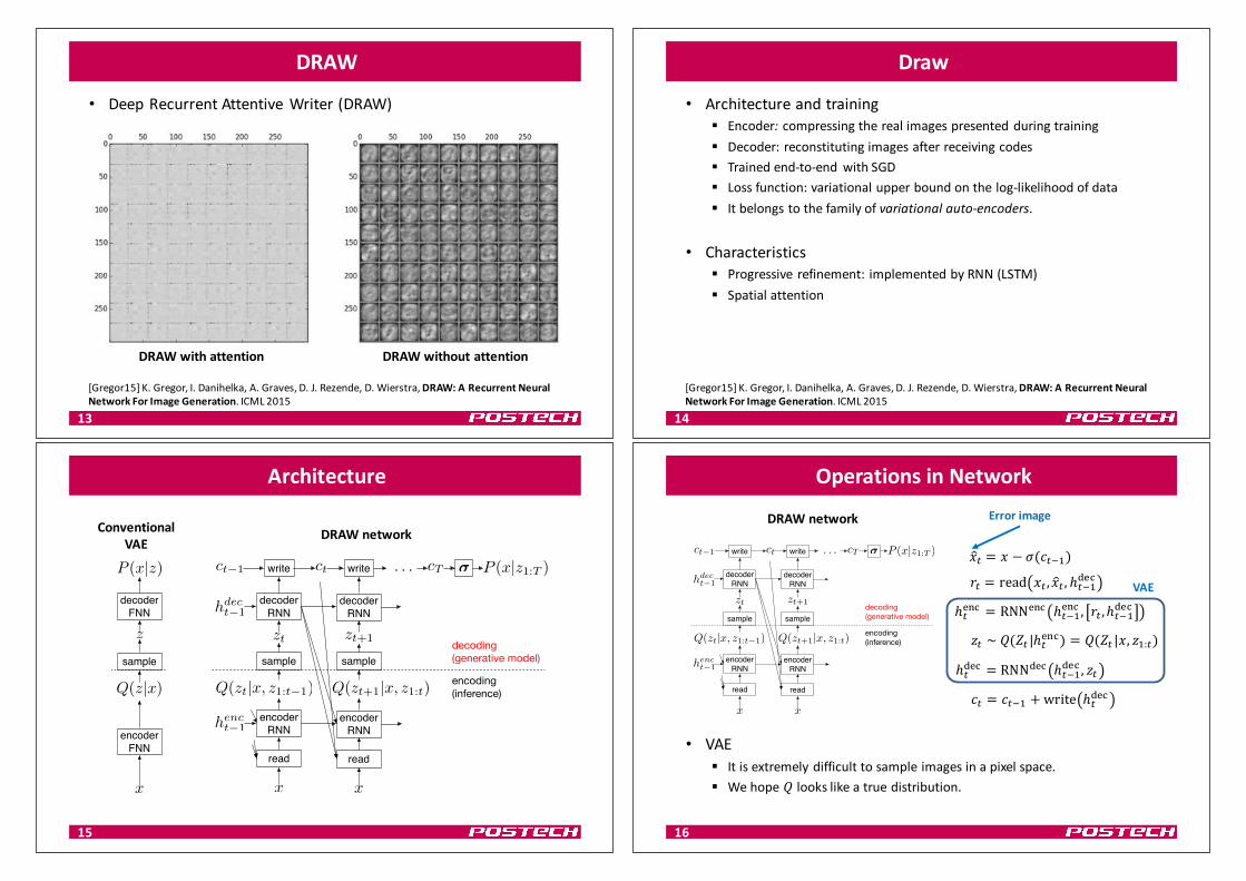
• DeepRecurrentAttentiveWriter(DRAW)§ Combinesaspatialattention

mechanismwithasequentialvariational auto-encodingframework

§ Allowsfortheiterativeconstructionofcompleximages

12

DRAW: A Recurrent Neural Network For Image Generation

Karol Gregor [email protected] Danihelka [email protected] Graves [email protected] Jimenez Rezende [email protected] Wierstra [email protected]

Google DeepMind

Abstract

This paper introduces the Deep Recurrent Atten-tive Writer (DRAW) neural network architecturefor image generation. DRAW networks combinea novel spatial attention mechanism that mimicsthe foveation of the human eye, with a sequentialvariational auto-encoding framework that allowsfor the iterative construction of complex images.The system substantially improves on the stateof the art for generative models on MNIST, and,when trained on the Street View House Numbersdataset, it generates images that cannot be distin-guished from real data with the naked eye.

1. IntroductionA person asked to draw, paint or otherwise recreate a visualscene will naturally do so in a sequential, iterative fashion,reassessing their handiwork after each modification. Roughoutlines are gradually replaced by precise forms, lines aresharpened, darkened or erased, shapes are altered, and thefinal picture emerges. Most approaches to automatic im-age generation, however, aim to generate entire scenes atonce. In the context of generative neural networks, this typ-ically means that all the pixels are conditioned on a singlelatent distribution (Dayan et al., 1995; Hinton & Salakhut-dinov, 2006; Larochelle & Murray, 2011). As well as pre-cluding the possibility of iterative self-correction, the “oneshot” approach is fundamentally difficult to scale to largeimages. The Deep Recurrent Attentive Writer (DRAW) ar-chitecture represents a shift towards a more natural form ofimage construction, in which parts of a scene are createdindependently from others, and approximate sketches aresuccessively refined.

Proceedings of the 32nd International Conference on MachineLearning, Lille, France, 2015. JMLR: W&CP volume 37. Copy-right 2015 by the author(s).

Time

Figure 1. A trained DRAW network generating MNIST dig-its. Each row shows successive stages in the generation of a sin-gle digit. Note how the lines composing the digits appear to be“drawn” by the network. The red rectangle delimits the area at-tended to by the network at each time-step, with the focal preci-sion indicated by the width of the rectangle border.

The core of the DRAW architecture is a pair of recurrentneural networks: an encoder network that compresses thereal images presented during training, and a decoder thatreconstitutes images after receiving codes. The combinedsystem is trained end-to-end with stochastic gradient de-scent, where the loss function is a variational upper boundon the log-likelihood of the data. It therefore belongs to thefamily of variational auto-encoders, a recently emergedhybrid of deep learning and variational inference that hasled to significant advances in generative modelling (Gre-gor et al., 2014; Kingma & Welling, 2014; Rezende et al.,2014; Mnih & Gregor, 2014; Salimans et al., 2014). WhereDRAW differs from its siblings is that, rather than generat-

[Gregor15]K.Gregor,I.Danihelka,A.Graves,D.J.Rezende,D.Wierstra,DRAW:ARecurrentNeuralNetworkForImageGeneration.ICML2015

DRAW

13

• DeepRecurrentAttentiveWriter(DRAW)


DRAWwithoutattentionDRAWwithattention

Draw

• Architectureandtraining§ Encoder:compressingtherealimagespresentedduringtraining§ Decoder:reconstitutingimagesafterreceivingcodes§ Trainedend-to-endwithSGD§ Lossfunction:variational upperboundonthelog-likelihoodofdata§ Itbelongstothefamilyofvariational auto-encoders.

• Characteristics§ Progressive refinement:implementedbyRNN(LSTM)§ Spatialattention

14


Architecture

15

DRAWnetworkDRAW: A Recurrent Neural Network For Image Generation

ing images in a single pass, it iteratively constructs scenesthrough an accumulation of modifications emitted by thedecoder, each of which is observed by the encoder.

An obvious correlate of generating images step by step isthe ability to selectively attend to parts of the scene whileignoring others. A wealth of results in the past few yearssuggest that visual structure can be better captured by a se-quence of partial glimpses, or foveations, than by a sin-gle sweep through the entire image (Larochelle & Hinton,2010; Denil et al., 2012; Tang et al., 2013; Ranzato, 2014;Zheng et al., 2014; Mnih et al., 2014; Ba et al., 2014; Ser-manet et al., 2014). The main challenge faced by sequentialattention models is learning where to look, which can beaddressed with reinforcement learning techniques such aspolicy gradients (Mnih et al., 2014). The attention model inDRAW, however, is fully differentiable, making it possibleto train with standard backpropagation. In this sense it re-sembles the selective read and write operations developedfor the Neural Turing Machine (Graves et al., 2014).

The following section defines the DRAW architecture,along with the loss function used for training and the pro-cedure for image generation. Section 3 presents the selec-tive attention model and shows how it is applied to read-ing and modifying images. Section 4 provides experi-mental results on the MNIST, Street View House Num-bers and CIFAR-10 datasets, with examples of generatedimages; and concluding remarks are given in Section 5.Lastly, we would like to direct the reader to the videoaccompanying this paper (https://www.youtube.com/watch?v=Zt-7MI9eKEo) which contains exam-ples of DRAW networks reading and generating images.

2. The DRAW NetworkThe basic structure of a DRAW network is similar to that ofother variational auto-encoders: an encoder network deter-mines a distribution over latent codes that capture salientinformation about the input data; a decoder network re-ceives samples from the code distribuion and uses them tocondition its own distribution over images. However thereare three key differences. Firstly, both the encoder and de-coder are recurrent networks in DRAW, so that a sequenceof code samples is exchanged between them; moreover theencoder is privy to the decoder’s previous outputs, allow-ing it to tailor the codes it sends according to the decoder’sbehaviour so far. Secondly, the decoder’s outputs are suc-cessively added to the distribution that will ultimately gen-erate the data, as opposed to emitting this distribution ina single step. And thirdly, a dynamically updated atten-tion mechanism is used to restrict both the input regionobserved by the encoder, and the output region modifiedby the decoder. In simple terms, the network decides ateach time-step “where to read” and “where to write” as well

read

write

encoderRNN

sample

decoderRNN

read

write

encoderRNN

sample

decoderRNN

c

t�1

c

t

c

T

�

h

enc

t�1

h

dec

t�1

Q(z

t+1

|x, z

1:t

)

. . .

decoding(generative model)

encoding(inference)

x

encoderFNN

sample

decoderFNN

z

Q(z|x)

P (x|z)

Figure 2. Left: Conventional Variational Auto-Encoder. Dur-ing generation, a sample z is drawn from a prior P (z) and passedthrough the feedforward decoder network to compute the proba-bility of the input P (x|z) given the sample. During inference theinput x is passed to the encoder network, producing an approx-imate posterior Q(z|x) over latent variables. During training, zis sampled from Q(z|x) and then used to compute the total de-scription length KL

�Q(Z|x)||P (Z)

�� log(P (x|z)), which is

minimised with stochastic gradient descent. Right: DRAW Net-work. At each time-step a sample zt from the prior P (zt) ispassed to the recurrent decoder network, which then modifies partof the canvas matrix. The final canvas matrix cT is used to com-pute P (x|z1:T ). During inference the input is read at every time-step and the result is passed to the encoder RNN. The RNNs atthe previous time-step specify where to read. The output of theencoder RNN is used to compute the approximate posterior overthe latent variables at that time-step.

as “what to write”. The architecture is sketched in Fig. 2,alongside a feedforward variational auto-encoder.

2.1. Network Architecture

Let RNN enc be the function enacted by the encoder net-work at a single time-step. The output of RNN enc at timet is the encoder hidden vector h

enct

. Similarly the output ofthe decoder RNN dec at t is the hidden vector h

dect

. In gen-eral the encoder and decoder may be implemented by anyrecurrent neural network. In our experiments we use theLong Short-Term Memory architecture (LSTM; Hochreiter& Schmidhuber (1997)) for both, in the extended form withforget gates (Gers et al., 2000). We favour LSTM dueto its proven track record for handling long-range depen-dencies in real sequential data (Graves, 2013; Sutskeveret al., 2014). Throughout the paper, we use the notationb = W (a) to denote a linear weight matrix with bias fromthe vector a to the vector b.

At each time-step t, the encoder receives input from boththe image x and from the previous decoder hidden vectorh

dect�1

. The precise form of the encoder input depends on aread operation, which will be defined in the next section.The output h

enct

of the encoder is used to parameterise adistribution Q(Z

t

|henct

) over the latent vector z

t

. In our






read

x

zt zt+1

P (x|z1:T )write

encoderRNN

sample

decoderRNN

read

x

write

encoderRNN

sample

decoderRNN

c

t�1

c

t

c

T

�

h

enc

t�1

h

dec

t�1

Q(zt|x, z1:t�1) Q(z

t+1

|x, z

1:t

)

. . .


encoding(inference)

encoderFNN

sample

decoderFNN

z

P (x|z)


�Q(Z|x)||P (Z)






enct


dect



dect�1


enct


t

|henct


t

. In our

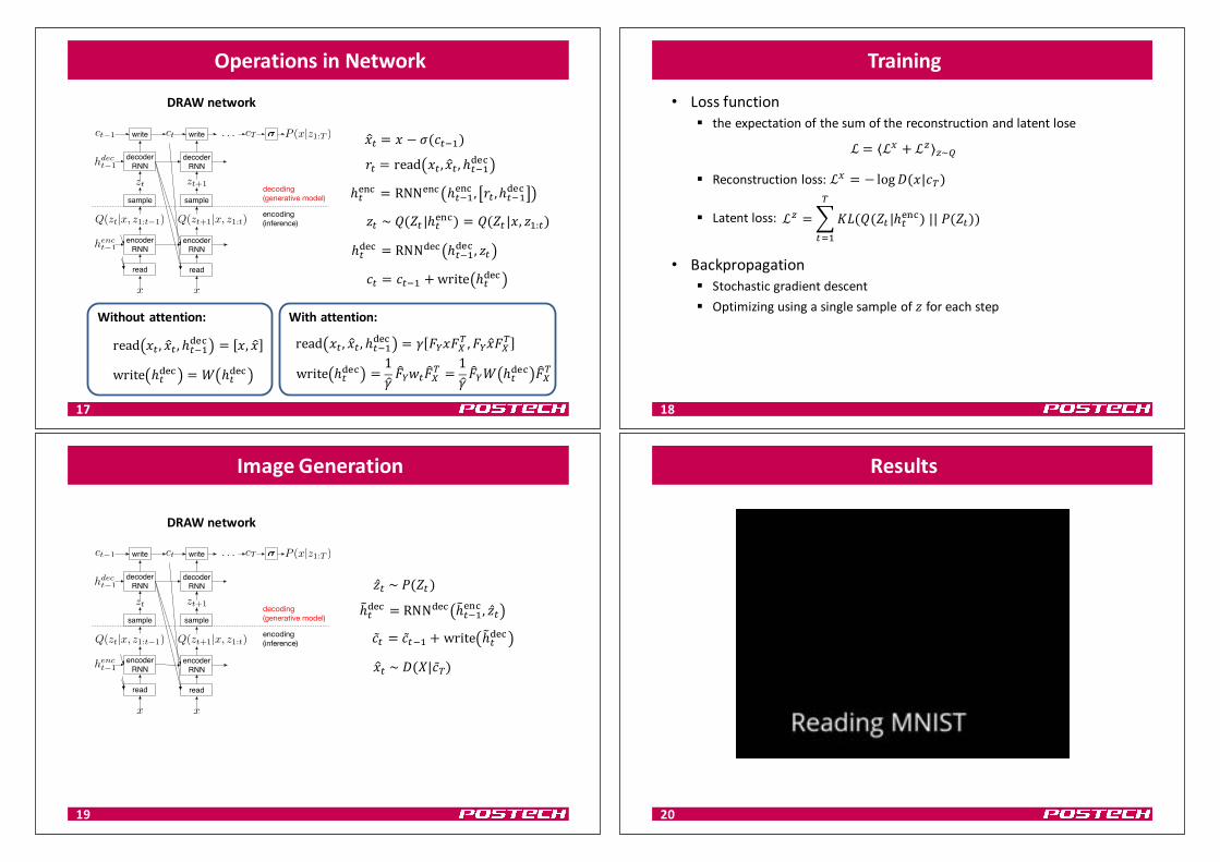
ConventionalVAE

• VAE§ Itisextremelydifficulttosampleimagesinapixelspace.§ WehopeC lookslikeatruedistribution.

OperationsinNetwork

16






read

x

zt zt+1

P (x|z1:T )write

encoderRNN

sample

decoderRNN

read

x

write

encoderRNN

sample

decoderRNN

c

t�1

c

t

c

T

�

h

enc

t�1

h

dec

t�1


t+1

|x, z

1:t

)

. . .


encoding(inference)

encoderFNN

sample

decoderFNN

z

P (x|z)


�Q(Z|x)||P (Z)






enct


dect



dect�1


enct


t

|henct


t

. In our

!DE = ! − F GEHI

JE = read !E, !DE, ℎEHIPQR

ℎEQSR = RNNQSR ℎEHI

QSR, JE, ℎEHI

PQR

"E ~C XE ℎEQSR = C XE !, "I:E

ℎEPQR = RNNPQR ℎEHI

PQR, "E

GE = GEHI + write ℎEPQR

ErrorimageDRAWnetwork

VAE






read

x

zt zt+1

P (x|z1:T )write

encoderRNN

sample

decoderRNN

read

x

write

encoderRNN

sample

decoderRNN

c

t�1

c

t

c

T

�

h

enc

t�1

h

dec

t�1


t+1

|x, z

1:t

)

. . .


encoding(inference)

encoderFNN

sample

decoderFNN

z

P (x|z)


�Q(Z|x)||P (Z)






enct


dect



dect�1


enct


t

|henct


t

. In our

OperationsinNetwork

17

DRAWnetwork

write ℎEPQR =

1

D_abE_c

d=1

D_ae ℎE

PQR _cd

read !E, !DE, ℎEHIPQR

= ^ _a!_cd, _a!D_c

d

Withattention:

write ℎEPQR = e ℎE

PQR

read !E, !DE, ℎEHIPQR

= !, !D

Withoutattention:

!DE = ! − F GEHI

JE = read !E, !DE, ℎEHIPQR

ℎEQSR = RNNQSR ℎEHI

QSR, JE, ℎEHI

PQR

ℎEPQR = RNNPQR ℎEHI

PQR, "E

GE = GEHI + write ℎEPQR

"E ~C XE ℎEQSR = C XE !, "I:E

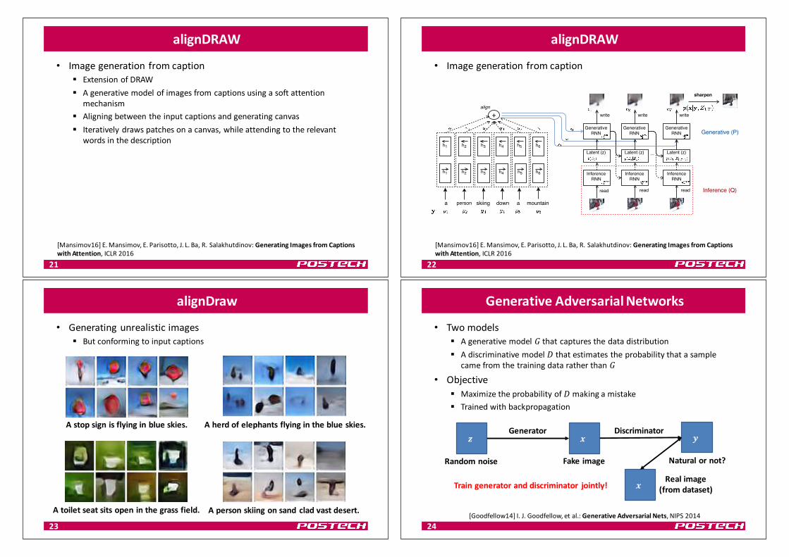
Training

• Lossfunction§ theexpectationofthesumofthereconstructionandlatentlose

§ Reconstructionloss:ℒf = − log@ ! Gd

§ Latentloss:

• Backpropagation§ Stochasticgradientdescent§ Optimizingusingasinglesampleof" foreachstep

18

ℒ = ℒf + ℒg g~h

ℒg =ijk C XE ℎEQSR ||l(XE)

d

EmI

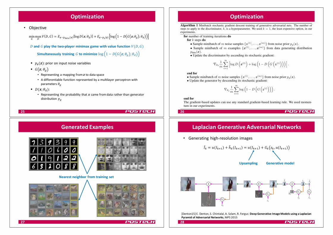
ImageGeneration

19






read

x

zt zt+1

P (x|z1:T )write

encoderRNN

sample

decoderRNN

read

x

write

encoderRNN

sample

decoderRNN

c

t�1

c

t

c

T

�

h

enc

t�1

h

dec

t�1


t+1

|x, z

1:t

)

. . .


encoding(inference)

encoderFNN

sample

decoderFNN

z

P (x|z)


�Q(Z|x)||P (Z)






enct


dect



dect�1


enct


t

|henct


t

. In our

DRAWnetwork

"E~l XE

GE = GEHI + write ℎpEPQR

ℎpEPQR = RNNPQR ℎpEHI

QSR, "E

!DE~@ q|Gd

Results

20

alignDRAW

• Imagegenerationfromcaption§ ExtensionofDRAW§ Agenerativemodelofimagesfromcaptionsusingasoftattention

mechanism§ Aligningbetweentheinputcaptionsandgeneratingcanvas§ Iterativelydrawspatchesonacanvas,whileattendingtotherelevant

wordsinthedescription

21

[Mansimov16]E.Mansimov,E.Parisotto,J.L.Ba,R.Salakhutdinov:GeneratingImagesfromCaptionswithAttention,ICLR2016

alignDRAW

• Imagegenerationfromcaption

22

Published as a conference paper at ICLR 2016

Figure 2: AlignDRAW model for generating images by learning an alignment between the input captions andgenerating canvas. The caption is encoded using the Bidirectional RNN (left). The generative RNN takes alatent sequence z1:T sampled from the prior along with the dynamic caption representation s1:T to generatethe canvas matrix cT , which is then used to generate the final image x (right). The inference RNN is used tocompute approximate posterior Q over the latent sequence.

3.2 IMAGE MODEL: THE CONDITIONAL DRAW NETWORK

To generate an image x conditioned on the caption information y, we extended the DRAW net-work (Gregor et al., 2015) to include caption representation h

lang at each step, as shown in Fig. 2.The conditional DRAW network is a stochastic recurrent neural network that consists of a sequenceof latent variables Z

t

2 RD, t = 1, .., T , where the output is accumulated over all T time-steps. Forsimplicity in notation, the images x 2 Rh⇥w are assumed to have size h-by-w and only one colorchannel.

Unlike the original DRAW network where latent variables are independent spherical GaussiansN (0, I), the latent variables in the proposed alignDRAW model have their mean and variance de-pend on the previous hidden states of the generative LSTM h

gen

t�1, except for P (Z1) = N (0, I).Namely, the mean and variance of the prior distribution over Z

t

are parameterized by:

P (Z

t

|Z1:t�1) = N✓µ(h

gen

t�1),�(hgen

t�1)

◆,

µ(h

gen

t�1) = tanh(W

µ

h

gen

t�1),

�(h

gen

t�1) = exp

�tanh(W

�

h

gen

t�1)�,

where W

µ

2 RD⇥n, W�

2 RD⇥n are the learned model parameters, and n is the dimensional-ity of hgen

t

, the hidden state of the generative LSTM. Similar to (Bachman & Precup, 2015), wehave observed that the model performance is improved by including dependencies between latentvariables.

Formally, an image is generated by iteratively computing the following set of equations for t =

1, ..., T (see Fig. 2), with h

gen

0 and c0 initialized to learned biases:

z

t

⇠ P (Z

t

|Z1:t�1) = N✓µ(h

gen

t�1),�(hgen

t�1)

◆, (1)

s

t

= align(h

gen

t�1, hlang

), (2)h

gen

t

= LSTM gen

(h

gen

t�1, [zt, st]), (3)c

t

= c

t�1 + write(hgen

t

), (4)

˜

x ⇠ P (x |y, Z1:T ) =

Y

i

P (x

i

|y, Z1:T ) =

Y

i

Bern(�(cT,i

)). (5)

The align function is used to compute the alignment between the input caption and intermediateimage generative steps (Bahdanau et al., 2015). Given the caption representation from the languagemodel, hlang

= [h

lang

1 , h

lang

2 , ..., h

lang

N

], the align operator outputs a dynamic sentence representa-tion s

t

at each step through a weighted sum using alignment probabilities ↵t

1...N :

s

t

= align(h

gen

t�1, hlang

) = ↵

t

1hlang

1 + ↵

t

2hlang

2 + ...+ ↵

t

N

h

lang

N

. (6)

3

[Mansimov16]E.Mansimov,E.Parisotto,J.L.Ba,R.Salakhutdinov:GeneratingImagesfromCaptionswithAttention,ICLR2016

alignDraw

• Generatingunrealisticimages§ Butconformingtoinputcaptions

23

Atoiletseatsitsopeninthegrassfield.


A stop sign is flying inblue skies.

A herd of elephants fly-ing in the blue skies.

A toilet seat sits open inthe grass field.

A person skiing on sandclad vast desert.

Figure 1: Examples of generated images based on captions that describe novel scene compositions that arehighly unlikely to occur in real life. The captions describe a common object doing unusual things or set in astrange location.

2 RELATED WORK

Deep Neural Networks have achieved significant success in various tasks such as image recognition(Krizhevsky et al., 2012), speech transcription (Graves et al., 2013), and machine translation (Bah-danau et al., 2015). While most of the recent success has been achieved by discriminative models,generative models have not yet enjoyed the same level of success. Most of the previous work ingenerative models has focused on variants of Boltzmann Machines (Smolensky, 1986; Salakhutdi-nov & Hinton, 2009) and Deep Belief Networks (Hinton et al., 2006). While these models are verypowerful, each iteration of training requires a computationally costly step of MCMC to approximatederivatives of an intractable partition function (normalization constant), making it difficult to scalethem to large datasets.

Kingma & Welling (2014), Rezende et al. (2014) have introduced the Variational Auto-Encoder(VAE) which can be seen as a neural network with continuous latent variables. The encoder is usedto approximate a posterior distribution and the decoder is used to stochastically reconstruct the datafrom latent variables. Gregor et al. (2015) further introduced the Deep Recurrent Attention Writer(DRAW), extending the VAE approach by incorporating a novel differentiable attention mechanism.

Generative Adversarial Networks (GANs) (Goodfellow et al., 2014) are another type of generativemodels that use noise-contrastive estimation (Gutmann & Hyvarinen, 2010) to avoid calculatingan intractable partition function. The model consists of a generator that generates samples usinga uniform distribution and a discriminator that discriminates between real and generated images.Recently, Denton et al. (2015) have scaled those models by training conditional GANs at each levelof a Laplacian pyramid of images.

While many of the previous approaches have focused on unconditional models or models condi-tioned on labels, in this paper we develop a generative model of images conditioned on captions.

3 MODEL

Our proposed model defines a generative process of images conditioned on captions. In particular,captions are represented as a sequence of consecutive words and images are represented as a se-quence of patches drawn on a canvas c

t

over time t = 1, ..., T . The model can be viewed as a partof the sequence-to-sequence framework (Sutskever et al., 2014; Cho et al., 2014; Srivastava et al.,2015).

3.1 LANGUAGE MODEL: THE BIDIRECTIONAL ATTENTION RNN

Let y be the input caption, represented as a sequence of 1-of-K encoded words y = (y1, y2, ..., yN ),where K is the size of the vocabulary and N is the length of the sequence. We obtain the caption sen-tence representation by first transforming each word y

i

to an m-dimensional vector representationh

lang

i

, i = 1, .., N using the Bidirectional RNN. In a Bidirectional RNN, the two LSTMs (Hochre-iter & Schmidhuber, 1997) with forget gates (Gers et al., 2000) process the input sequence from bothforward and backward directions. The Forward LSTM computes the sequence of forward hiddenstates [

�!h

lang

1 ,

�!h

lang

2 , ...,

�!h

lang

N

] , whereas the Backward LSTM computes the sequence of back-ward hidden states [

�h

lang

1 ,

�h

lang

2 , ...,

�h

lang

N

]. These hidden states are then concatenated togetherinto the sequence h

lang

= [h

lang

1 , h

lang

2 , ..., h

lang

N

], with h

lang

i

= [

�!h

lang

i

,

�h

lang

i

], 1 i N .

2

Apersonskiingonsandcladvastdesert.







2 RELATED WORK





3 MODEL


t




i


lang

i


�!h

lang

1 ,

�!h

lang

2 , ...,

�!h

lang

N


�h

lang

1 ,

�h

lang

2 , ...,

�h

lang

N


lang

= [h

lang

1 , h

lang

2 , ..., h

lang

N

], with h

lang

i

= [

�!h

lang

i

,

�h

lang

i

], 1 i N .

2







2 RELATED WORK





3 MODEL


t




i


lang

i


�!h

lang

1 ,

�!h

lang

2 , ...,

�!h

lang

N


�h

lang

1 ,

�h

lang

2 , ...,

�h

lang

N


lang

= [h

lang

1 , h

lang

2 , ..., h

lang

N

], with h

lang

i

= [

�!h

lang

i

,

�h

lang

i

], 1 i N .

2

Astopsignisflyinginblueskies.







2 RELATED WORK





3 MODEL


t




i


lang

i


�!h

lang

1 ,

�!h

lang

2 , ...,

�!h

lang

N


�h

lang

1 ,

�h

lang

2 , ...,

�h

lang

N


lang

= [h

lang

1 , h

lang

2 , ..., h

lang

N

], with h

lang

i

= [

�!h

lang

i

,

�h

lang

i

], 1 i N .

2

Aherdofelephantsflyingintheblueskies.

GenerativeAdversarialNetworks

• Twomodels§ A generativemodelr thatcapturesthedatadistribution§ Adiscriminativemodel @ thatestimatestheprobabilitythatasample

camefromthetrainingdataratherthanr

• Objective§ Maximizetheprobabilityof@ makingamistake§ Trainedwithbackpropagation

24

) 0

FakeimageRandomnoise

Generators

Discriminator

Naturalornot?

0Realimage

(fromdataset)Traingeneratoranddiscriminator jointly!

[Goodfellow14]I.J.Goodfellow,etal.:GenerativeAdversarialNets,NIPS2014

Optimization

• Objective

§ +) ) :prioroninputnoisevariables

§ r ); (t

• Representingamappingfrom)todataspace• Adifferentiablefunctionrepresentedbyamultilayerperceptronwithparameters(t

§ @ 0; (u :• Representingtheprobabilitythat0 camefromdataratherthangeneratordistribution+t

25

minxmaxz

{ @, r = 90~|}~�~ 0 log@ 0; (u + 9)~|) ) log 1 − @ r );(t ; (u

Simultaneously trainingr tominimizelog 1 − @ r ); (t ; (u

@ andr playthetwo-playerminimaxgamewithvaluefunction{ @, r

Optimization

26

. . .

(a) (b) (c) (d)

Figure 1: Generative adversarial nets are trained by simultaneously updating the discriminative distribution(D, blue, dashed line) so that it discriminates between samples from the data generating distribution (black,dotted line) p

x

from those of the generative distribution pg (G) (green, solid line). The lower horizontal line isthe domain from which z is sampled, in this case uniformly. The horizontal line above is part of the domainof x. The upward arrows show how the mapping x = G(z) imposes the non-uniform distribution pg ontransformed samples. G contracts in regions of high density and expands in regions of low density of pg . (a)Consider an adversarial pair near convergence: pg is similar to pdata and D is a partially accurate classifier.(b) In the inner loop of the algorithm D is trained to discriminate samples from data, converging to D

⇤(x) =pdata(x)

pdata(x)+pg(x) . (c) After an update to G, gradient of D has guided G(z) to flow to regions that are more likelyto be classified as data. (d) After several steps of training, if G and D have enough capacity, they will reach apoint at which both cannot improve because pg = pdata. The discriminator is unable to differentiate betweenthe two distributions, i.e. D(x) = 1

2 .

Algorithm 1 Minibatch stochastic gradient descent training of generative adversarial nets. The number ofsteps to apply to the discriminator, k, is a hyperparameter. We used k = 1, the least expensive option, in ourexperiments.

for number of training iterations dofor k steps do

• Sample minibatch of m noise samples {z(1), . . . , z

(m)} from noise prior pg

(z).• Sample minibatch of m examples {x(1)

, . . . ,x

(m)} from data generating distributionpdata(x).• Update the discriminator by ascending its stochastic gradient:

r✓d

1

m

mX

i=1

hlogD

⇣x

(i)⌘+ log

⇣1�D

⇣G

⇣z

(i)⌘⌘⌘i

.

end for• Sample minibatch of m noise samples {z(1)

, . . . , z

(m)} from noise prior pg

(z).• Update the generator by descending its stochastic gradient:

r✓g

1

m

mX

i=1

log

⇣1�D

⇣G

⇣z

(i)⌘⌘⌘

.

end forThe gradient-based updates can use any standard gradient-based learning rule. We used momen-tum in our experiments.

4.1 Global Optimality of pg

= pdata

We first consider the optimal discriminator D for any given generator G.

Proposition 1. For G fixed, the optimal discriminator D is

D

⇤

G

(x) =

p

data

(x)

p

data

(x) + p

g

(x)

(2)

4

GeneratedExamples

27

a) b)

c) d)

Figure 2: Visualization of samples from the model. Rightmost column shows the nearest training example ofthe neighboring sample, in order to demonstrate that the model has not memorized the training set. Samplesare fair random draws, not cherry-picked. Unlike most other visualizations of deep generative models, theseimages show actual samples from the model distributions, not conditional means given samples of hidden units.Moreover, these samples are uncorrelated because the sampling process does not depend on Markov chainmixing. a) MNIST b) TFD c) CIFAR-10 (fully connected model) d) CIFAR-10 (convolutional discriminatorand “deconvolutional” generator)

Figure 3: Digits obtained by linearly interpolating between coordinates in z space of the full model.

1. A conditional generative model p(x | c) can be obtained by adding c as input to both G and D.2. Learned approximate inference can be performed by training an auxiliary network to predict z

given x. This is similar to the inference net trained by the wake-sleep algorithm [15] but withthe advantage that the inference net may be trained for a fixed generator net after the generatornet has finished training.

3. One can approximately model all conditionals p(x

S

| x6S

) where S is a subset of the indicesof x by training a family of conditional models that share parameters. Essentially, one can useadversarial nets to implement a stochastic extension of the deterministic MP-DBM [10].

4. Semi-supervised learning: features from the discriminator or inference net could improve perfor-mance of classifiers when limited labeled data is available.

5. Efficiency improvements: training could be accelerated greatly by devising better methods forcoordinating G and D or determining better distributions to sample z from during training.

This paper has demonstrated the viability of the adversarial modeling framework, suggesting thatthese research directions could prove useful.

7

a)b)

c)d)

Figure2:Visualizationofsamplesfromthemodel.Rightmostcolumnshowsthenearesttrainingexampleoftheneighboringsample,inordertodemonstratethatthemodelhasnotmemorizedthetrainingset.Samplesarefairrandomdraws,notcherry-picked.Unlikemostothervisualizationsofdeepgenerativemodels,theseimagesshowactualsamplesfromthemodeldistributions,notconditionalmeansgivensamplesofhiddenunits.Moreover,thesesamplesareuncorrelatedbecausethesamplingprocessdoesnotdependonMarkovchainmixing.a)MNISTb)TFDc)CIFAR-10(fullyconnectedmodel)d)CIFAR-10(convolutionaldiscriminatorand“deconvolutional”generator)

Figure3:Digitsobtainedbylinearlyinterpolatingbetweencoordinatesinzspaceofthefullmodel.

1.Aconditionalgenerativemodelp(x|c)canbeobtainedbyaddingcasinputtobothGandD.2.Learnedapproximateinferencecanbeperformedbytraininganauxiliarynetworktopredictz

givenx.Thisissimilartotheinferencenettrainedbythewake-sleepalgorithm[15]butwiththeadvantagethattheinferencenetmaybetrainedforafixedgeneratornetafterthegeneratornethasfinishedtraining.

3.Onecanapproximatelymodelallconditionalsp(x

S

|x6S

)whereSisasubsetoftheindicesofxbytrainingafamilyofconditionalmodelsthatshareparameters.Essentially,onecanuseadversarialnetstoimplementastochasticextensionofthedeterministicMP-DBM[10].

4.Semi-supervisedlearning:featuresfromthediscriminatororinferencenetcouldimproveperfor-manceofclassifierswhenlimitedlabeleddataisavailable.

5.Efficiencyimprovements:trainingcouldbeacceleratedgreatlybydevisingbettermethodsforcoordinatingGandDordeterminingbetterdistributionstosamplezfromduringtraining.

Thispaperhasdemonstratedtheviabilityoftheadversarialmodelingframework,suggestingthattheseresearchdirectionscouldproveuseful.

7

a)b)

c)d)

Figure2:Visualizationofsamplesfromthemodel.Rightmostcolumnshowsthenearesttrainingexampleoftheneighboringsample,inordertodemonstratethatthemodelhasnotmemorizedthetrainingset.Samplesarefairrandomdraws,notcherry-picked.Unlikemostothervisualizationsofdeepgenerativemodels,theseimagesshowactualsamplesfromthemodeldistributions,notconditionalmeansgivensamplesofhiddenunits.Moreover,thesesamplesareuncorrelatedbecausethesamplingprocessdoesnotdependonMarkovchainmixing.a)MNISTb)TFDc)CIFAR-10(fullyconnectedmodel)d)CIFAR-10(convolutionaldiscriminatorand“deconvolutional”generator)

Figure3:Digitsobtainedbylinearlyinterpolatingbetweencoordinatesinzspaceofthefullmodel.

1.Aconditionalgenerativemodelp(x|c)canbeobtainedbyaddingcasinputtobothGandD.2.Learnedapproximateinferencecanbeperformedbytraininganauxiliarynetworktopredictz

givenx.Thisissimilartotheinferencenettrainedbythewake-sleepalgorithm[15]butwiththeadvantagethattheinferencenetmaybetrainedforafixedgeneratornetafterthegeneratornethasfinishedtraining.

3.Onecanapproximatelymodelallconditionalsp(x

S

|x6S

)whereSisasubsetoftheindicesofxbytrainingafamilyofconditionalmodelsthatshareparameters.Essentially,onecanuseadversarialnetstoimplementastochasticextensionofthedeterministicMP-DBM[10].

4.Semi-supervisedlearning:featuresfromthediscriminatororinferencenetcouldimproveperfor-manceofclassifierswhenlimitedlabeleddataisavailable.

5.Efficiencyimprovements:trainingcouldbeacceleratedgreatlybydevisingbettermethodsforcoordinatingGandDordeterminingbetterdistributionstosamplezfromduringtraining.

Thispaperhasdemonstratedtheviabilityoftheadversarialmodelingframework,suggestingthattheseresearchdirectionscouldproveuseful.

7

a) b)

c) d)

Figure 2: Visualization of samples from the model. Rightmost column shows the nearest training example ofthe neighboring sample, in order to demonstrate that the model has not memorized the training set. Samplesare fair random draws, not cherry-picked. Unlike most other visualizations of deep generative models, theseimages show actual samples from the model distributions, not conditional means given samples of hidden units.Moreover, these samples are uncorrelated because the sampling process does not depend on Markov chainmixing. a) MNIST b) TFD c) CIFAR-10 (fully connected model) d) CIFAR-10 (convolutional discriminatorand “deconvolutional” generator)

Figure 3: Digits obtained by linearly interpolating between coordinates in z space of the full model.

1. A conditional generative model p(x | c) can be obtained by adding c as input to both G and D.2. Learned approximate inference can be performed by training an auxiliary network to predict z

given x. This is similar to the inference net trained by the wake-sleep algorithm [15] but withthe advantage that the inference net may be trained for a fixed generator net after the generatornet has finished training.

3. One can approximately model all conditionals p(x

S

| x6S

) where S is a subset of the indicesof x by training a family of conditional models that share parameters. Essentially, one can useadversarial nets to implement a stochastic extension of the deterministic MP-DBM [10].

4. Semi-supervised learning: features from the discriminator or inference net could improve perfor-mance of classifiers when limited labeled data is available.

5. Efficiency improvements: training could be accelerated greatly by devising better methods forcoordinating G and D or determining better distributions to sample z from during training.

This paper has demonstrated the viability of the adversarial modeling framework, suggesting thatthese research directions could prove useful.

7

Nearestneighbor fromtrainingset

LaplacianGenerativeAdversarialNetworks

• Generatinghigh-resolutionimages

28

ÄÅÇ = É ÄÇÑI + ℎÇ ÄÇÑI = É ÄÇÑI + rÇ "Ç , É ÄÇÑI

2.2 Laplacian Pyramid

The Laplacian pyramid [1] is a linear invertible image representation consisting of a set of band-passimages, spaced an octave apart, plus a low-frequency residual. Formally, let d(.) be a downsamplingoperation which blurs and decimates a j⇥ j image I , so that d(I) is a new image of size j/2⇥ j/2.Also, let u(.) be an upsampling operator which smooths and expands I to be twice the size, so u(I)is a new image of size 2j ⇥ 2j. We first build a Gaussian pyramid G(I) = [I0, I1, . . . , IK ], whereI0 = I and I

k

is k repeated applications of d(.) to I , i.e. I2 = d(d(I)). K is the number of levels inthe pyramid, selected so that the final level has very small spatial extent ( 8⇥ 8 pixels).

The coefficients hk

at each level k of the Laplacian pyramid L(I) are constructed by taking thedifference between adjacent levels in the Gaussian pyramid, upsampling the smaller one with u(.)so that the sizes are compatible:

hk

= Lk

(I) = Gk

(I)� u(Gk+1(I)) = I

k

� u(Ik+1) (3)

Intuitively, each level captures image structure present at a particular scale. The final level of theLaplacian pyramid h

K

is not a difference image, but a low-frequency residual equal to the finalGaussian pyramid level, i.e. h

K

= IK

. Reconstruction from a Laplacian pyramid coefficients[h1, . . . , hK

] is performed using the backward recurrence:Ik

= u(Ik+1) + h

k

(4)which is started with I

K

= hK

and the reconstructed image being I = Io

. In other words, startingat the coarsest level, we repeatedly upsample and add the difference image h at the next finer leveluntil we get back to the full resolution image.

2.3 Laplacian Generative Adversarial Networks (LAPGAN)

Our proposed approach combines the conditional GAN model with a Laplacian pyramid represen-tation. The model is best explained by first considering the sampling procedure. Following training(explained below), we have a set of generative convnet models {G0, . . . , GK

}, each of which cap-tures the distribution of coefficients h

k

for natural images at a different level of the Laplacian pyra-mid. Sampling an image is akin to the reconstruction procedure in Eqn. 4, except that the generativemodels are used to produce the h

k

’s:

˜Ik

= u(˜Ik+1) +

˜hk

= u(˜Ik+1) +G

k

(zk

, u(˜Ik+1)) (5)

The recurrence starts by setting ˜IK+1 = 0 and using the model at the final level G

K

to generate aresidual image ˜I

K

using noise vector zK

: ˜IK

= GK

(zK

). Note that models at all levels except thefinal are conditional generative models that take an upsampled version of the current image ˜I

k+1 asa conditioning variable, in addition to the noise vector z

k

. Fig. 1 shows this procedure in action fora pyramid with K = 3 using 4 generative models to sample a 64⇥ 64 image.

The generative models {G0, . . . , GK

} are trained using the CGAN approach at each level of thepyramid. Specifically, we construct a Laplacian pyramid from each training image I . At each levelwe make a stochastic choice (with equal probability) to either (i) construct the coefficients h

k

eitherusing the standard procedure from Eqn. 3, or (ii) generate them using G

k

:

˜hk

= Gk

(zk

, u(Ik+1)) (6)

G2

~ I3

G3

z2

~ h2

z3

G1

z1 G0

z0

~ I2 l2

~ I0

h0 ~

I1 ~

~ h1

l1

l0

Figure 1: The sampling procedure for our LAPGAN model. We start with a noise sample z3 (right side) anduse a generative model G3 to generate I3. This is upsampled (green arrow) and then used as the conditioningvariable (orange arrow) l2 for the generative model at the next level, G2. Together with another noise samplez2, G2 generates a difference image h2 which is added to l2 to create I2. This process repeats across twosubsequent levels to yield a final full resolution sample I0.

3

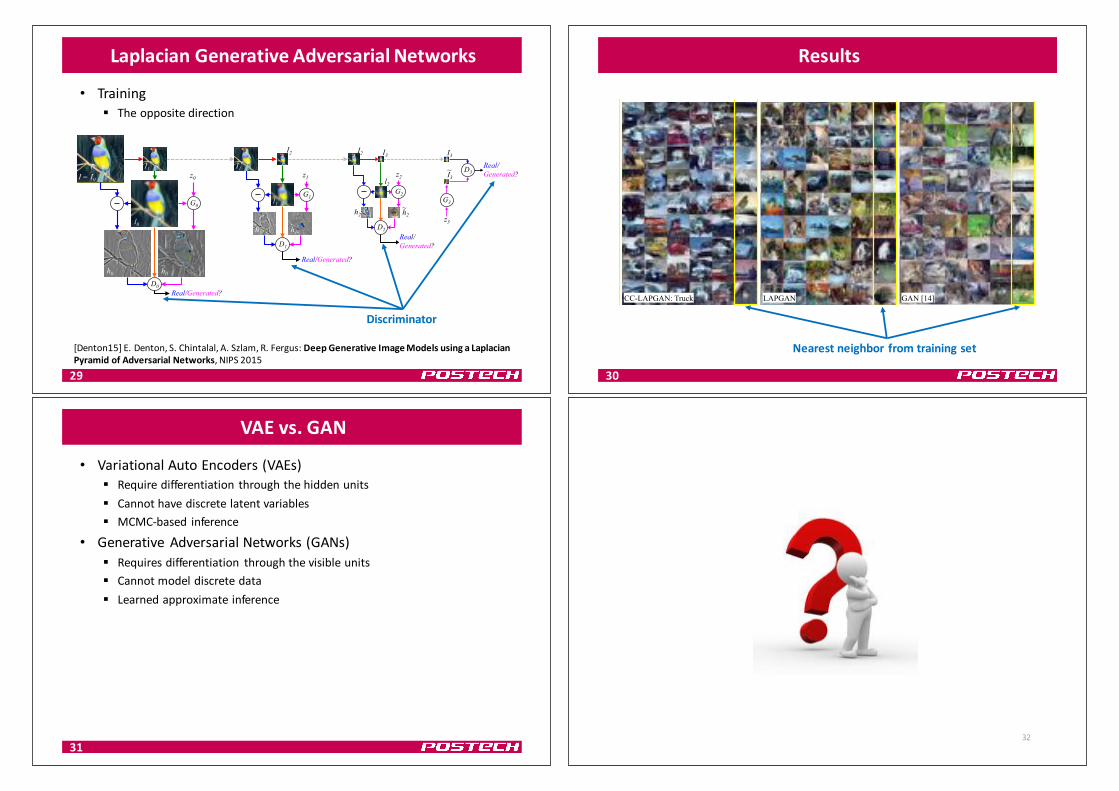
[Denton15]E.Denton,S.Chintalal,A.Szlam,R.Fergus:DeepGenerativeImageModelsusingaLaplacianPyramidofAdversarialNetworks,NIPS2015

Upsampling Generativemodel

LaplacianGenerativeAdversarialNetworks

• Training§ Theoppositedirection

29

G0

l2

~ I3

G3

D0

z0

D1

D2

h2 ~ h2 z3

D3

I3 I2 I2 I3

Real/Generated?

Real/ Generated?

G1

z1

G2

z2

Real/Generated?

Real/ Generated?

l0

I = I0

h0

I1 I1

l1

~ h1 h1

h0 ~

Figure 2: The training procedure for our LAPGAN model. Starting with a 64x64 input image I from ourtraining set (top left): (i) we take I0 = I and blur and downsample it by a factor of two (red arrow) to produceI1; (ii) we upsample I1 by a factor of two (green arrow), giving a low-pass version l0 of I0; (iii) with equalprobability we use l0 to create either a real or a generated example for the discriminative model D0. In the realcase (blue arrows), we compute high-pass h0 = I0 � l0 which is input to D0 that computes the probability ofit being real vs generated. In the generated case (magenta arrows), the generative network G0 receives as inputa random noise vector z0 and l0. It outputs a generated high-pass image h0 = G0(z0, l0), which is input toD0. In both the real/generated cases, D0 also receives l0 (orange arrow). Optimizing Eqn. 2, G0 thus learnsto generate realistic high-frequency structure h0 consistent with the low-pass image l0. The same procedure isrepeated at scales 1 and 2, using I1 and I2. Note that the models at each level are trained independently. Atlevel 3, I3 is an 8⇥8 image, simple enough to be modeled directly with a standard GANs G3 & D3.

Note that Gk

is a convnet which uses a coarse scale version of the image lk

= u(Ik+1) as an input,

as well as noise vector zk

. Dk

takes as input hk

or ˜hk

, along with the low-pass image lk

(which isexplicitly added to h

k

or ˜hk

before the first convolution layer), and predicts if the image was real orgenerated. At the final scale of the pyramid, the low frequency residual is sufficiently small that itcan be directly modeled with a standard GAN: ˜h

K

= GK

(zK

) and DK

only has hK

or ˜hK

as input.The framework is illustrated in Fig. 2.

Breaking the generation into successive refinements is the key idea in this work. Note that we giveup any “global” notion of fidelity; we never make any attempt to train a network to discriminatebetween the output of a cascade and a real image and instead focus on making each step plausible.Furthermore, the independent training of each pyramid level has the advantage that it is far moredifficult for the model to memorize training examples – a hazard when high capacity deep networksare used.

As described, our model is trained in an unsupervised manner. However, we also explore variantsthat utilize class labels. This is done by add a 1-hot vector c, indicating class identity, as anotherconditioning variable for G

k

and Dk

.

3 Model Architecture & TrainingWe apply our approach to three datasets: (i) CIFAR10 [17] – 32⇥32 pixel color images of 10different classes, 100k training samples with tight crops of objects; (ii) STL10 [2] – 96⇥96 pixelcolor images of 10 different classes, 100k training samples (we use the unlabeled portion of data);and (iii) LSUN [32] – ⇠10M images of 10 different natural scene types, downsampled to 64⇥64pixels.

For each dataset, we explored a variety of architectures for {Gk

, Dk

}. Model selection wasperformed using a combination of visual inspection and a heuristic based on `2 error in pixelspace. The heuristic computes the error for a given validation image at level k in the pyramidas L

k

(Ik

) = min{zj}||Gk

(zj

, u(Ik+1)) � h

k

||2 where {zj

} is a large set of noise vectors, drawnfrom p

noise

(z). In other words, the heuristic is asking, are any of the generated residual imagesclose to the ground truth? Torch training and evaluation code, along with model specification filescan be found at http://soumith.ch/eyescream/. For all models, the noise vector z

k

isdrawn from a uniform [-1,1] distribution.

4

[Denton15]E.Denton,S.Chintalal,A.Szlam,R.Fergus:DeepGenerativeImageModelsusingaLaplacianPyramidofAdversarialNetworks,NIPS2015

Discriminator

Results

30

CC-LAPGAN: Airplane CC-LAPGAN: Automobile CC-LAPGAN: Bird CC-LAPGAN: Cat

CC-LAPGAN: Deer CC-LAPGAN: Dog CC-LAPGAN: Frog CC-LAPGAN: Horse

CC-LAPGAN: Ship CC-LAPGAN: Truck GAN [14] LAPGAN

Figure 3: CIFAR10 samples: our class conditional CC-LAPGAN model, our LAPGAN model andthe standard GAN model of Goodfellow [11]. The yellow column shows the training set nearestneighbors of the samples in the adjacent column.

(a) (b)Figure 4: STL10 samples: (a) Random 96x96 samples from our LAPGAN model. (b) Coarse-to-fine generation chain.

7

Nearestneighbor fromtrainingset

VAEvs.GAN

• Variational AutoEncoders(VAEs)§ Requiredifferentiation throughthehiddenunits§ Cannothavediscretelatentvariables§ MCMC-based inference

• GenerativeAdversarialNetworks(GANs)§ Requiresdifferentiation throughthevisibleunits§ Cannotmodeldiscretedata§ Learnedapproximateinference

3132

Documents

Lecture 14: Deep Generative Learning Generative ...cvlab.postech.ac.kr/~bhhan/class/cse703r_2016s/... · Variational Autoencoder • Characteristics § A Bayesian approach on an autoencoder: