Embed Size (px)
Citation preview

Lecture 13
The Turbulent Burning Velocity
13.-1
The Turbulent Burning Velocity
One of the most important unresolved problems in premixed turbulent combustion is that of the turbulent burning velocity.
This statement implies that the turbulent burning velocity is a well-definedquantity that only depends on local mean quantities.
The mean turbulent flame front is expected to propagate with that burning velocity relative to the flow field.
Gas expansion effects induced at the mean front will change the surrounding flow field and may generate instabilities in a similar way as flame instabilities of the Darrieus-Landau type are generated by a laminar flame front (cf. Clavin, 1985).
13.-2

Damköhler (1940) was the first to present theoretical expressions for theturbulent burning velocity.
He identified two different regimes of premixed turbulent combustion which he called large scale and small scale turbulence.
We will identify these two regimes with the corrugated flamelets regime and the thin reaction zones regime, respectively.
13.-3

Damköhler equated the mass flux through the instantaneous turbulent flamesurface area AT with the mass flux through the cross sectional area A, using the laminar burning velocity sL for the mass flux through the instantaneous surface and the turbulent burning velocity sT for the mass flux through the cross-sectional area A as
The burning velocities sL and sT are defined with respect to the conditions in the unburnt mixture and the density ρu is assumed constant.
13.-4

From that equation it follows
Since only continuity is involved, averaging of the flame surface area can beperformed at any length scale Δ within the inertial range.
If Δ is interpreted as a filter width one obtains a filtered flame surface area
then also implies
This shows that the product is inertial range invariant, similar to the dissipation in the inertial range of turbulence.
13.-5

As a consequence, by analogy to the large Reynolds number limit used in turbulent modeling, the additional limit of the ratio of the turbulent to the laminar burning velocity for large values of v'/sL is the backbone of premixed turbulent combustion modeling.
For large scale turbulence, Damköhler (1940) assumed that the interaction between a wrinkled flame front and the turbulent flow field is purely kinematic.
Using the geometrical analogy with a Bunsen flame, he related the areaincrease of the wrinkled flame surface area to the velocity fluctuation divided by the laminar burning velocity
13.-6

Combining
and
leads to
in the limit of large v'/sL, which is a kinematic scaling.
We now want to show that this is consistent with the modeling assumption for the G-equation in the corrugated flamelets regime.
13.-7

For small scale turbulence, which we will identify with the thin reaction zones regime, Damköhler (1940) argued that turbulence only modifies the transport between the reaction zone and the unburnt gas.
In analogy to the scaling relation for the laminar burning velocity
where tc is the chemical time scale and D the molecular diffusivity, heproposes that the turbulent burning velocity can simply be obtained by replacing the laminar diffusivity D by the turbulent diffusivity Dt :
while the chemical time scale remains the same.
13.-8

Thereby it is implicitly assumed that the chemical time scale is not affected by turbulence.
This assumption breaks down when Kolmogorov eddies penetrate into the thin reaction zone. This implies that there is an upper limit for the thin reaction zones regime which was identified as the condition Kaδ = 1.
Combining
and
the ratio of the turbulent to the laminar burning velocity becomes
13.-9

Since the turbulent diffusivity DT is proportional to the product , and the laminar diffusivity is proportional to the product of the laminar burning velocity and the flame thickness one may write
as
showing that for small scale turbulence the burning velocity ratio not only depends on the velocity ratio v'/sL but also on the length scale ratio
13.-10

There were many attempts to modify Damköhler's analysis and to derive expressions that would reproduce the large amount of experimental data on turbulent burning velocities.
By introducing an adjustable exponent n, where 0.5 < n < 1.0
and
may be combined to obtain expressions of the form
This includes the limit v‘ → 0 for laminar flame propagation where sT=sL.
The constant C is expected to depend on the length scale ratio
13.-11

By comparison with experiments the exponent n is often found to be in the vicinity of 0.7 (cf. Williams ,1985).
Attempts to justify a single exponent on the basis of dimensional analysis, however, fall short even of Damköhler's pioneering work who had recognized the existence of two different regimes in premixed turbulent combustion.

There is a large amount of data on turbulent burning velocities in the literature.
Correlations of this material, mostly presented in terms of the burning velocity ratio sT/sL
plotted as a function of v'/sL, called the burning velocity diagram.
When experimental data fromdifferent authors are collected in such a diagram, they usually differ considerably. In the review articles by Bray (1990) and Bradley (1992) the many physical parameters that affect the turbulent burning velocity are discussed.
13.-13

A Model Equation for the Flame Surface Area Ratio
It was stated previously that the mean gradient represents the flame surface area ratio.
In the two-dimensional illustration the instantaneous flamesurface area AT is identified with the length of the line G=G0.
The blow-up shows that a differential section dS of that line and thecorresponding differential section dy of the cross sectional area A are related to each other by
13.-14

On the other hand, in two dimensions the gradient σ is given by
It can be seen that which relates σ to the angle β as
and therefore
the differential flame surface area ratio is equal to the gradient σ:
13.-15
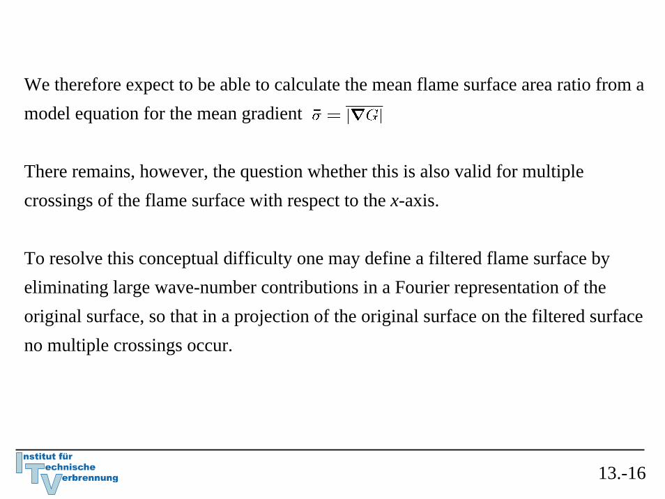
We therefore expect to be able to calculate the mean flame surface area ratio from a model equation for the mean gradient
There remains, however, the question whether this is also valid for multiple crossings of the flame surface with respect to the x-axis.
To resolve this conceptual difficulty one may define a filtered flame surface by eliminating large wave-number contributions in a Fourier representation of the original surface, so that in a projection of the original surface on the filtered surface no multiple crossings occur.
13.-16

This is also shown in the illustration.
The normal co-ordinate xn on the filtered surface then corresponds to x in a previous figure repeated here.
This shows that the ansatzAssuming a single valued function of x is again applicable.
A successive filtering procedure can then be applied, so that theflame surface area ratio is related to at each level of filtering.
13.-17

Within a given section dy
is then replaced by
where ν is an iteration index of successive filtering.
The quantities dS0 and σ0 correspond to the instantaneous differential flame surface area dS and the respective gradient σ, and dS1 and σ1 to those of the first filtering level.
At the next iteration one has dS1/dS2=σ1/σ2 and so on.
13.-18

At the last filtering level for ν → ∞ the flame surface becomes parallel to the y-co-ordinate, so that dS∞ = dy and σ∞ =1.
Canceling all intermediate iterations we obtain again
This analysis assumes that the original flame surface is unique and continuous.
13.-19

We now want to derive a modeled equation for the flame surface area ratio in order to determine the turbulent burning velocity.
An equation for σ can be derived from
For illustration purpose we assume constant density and constant values of sL
0 and D.
13.-20

Applying the Nabla-operator to both sides of
multiplying this with
one obtains
The terms on the l.h.s. of this equation describe the unsteady change and convection of σ.
The first term on the r.h.s accounts for straining by the flow field which amounts to a production of flame surface area.
13.-21

The second term on the r.h.s. containing the laminar burning velocity has asimilar effect as kinematic restoration has in the variance equation.
The last term is proportional to D and its effect is similar to that of scalar dissipation in the variance equation.
In order to derive a model equation for the mean value of σ we could, in principle, take the appropriate averages.
There is, however, no standard two-point closure procedure of such an equation, as there is none for deriving the ε-equation from an equation for the viscous dissipation.
13.-22

Therefore another approach was adopted in Peters (1999):
The scaling relations between ,were used separately in both regimes to derive the quation from a combination of the -equations.
The resulting equations contain the local change and convection of , a production term by mean gradients and another due to turbulence.
However, each of them contains a different sink term: In the corrugated flamelets regime the sink term is proportional to and in the thin reaction zones it is proportional to
13.-23

Since proportionality between the turbulent burning velocity and is valid only in the limit of large values of v'/sL, it accounts only for the increase of the flame surface area ratio due to turbulence, beyond the laminar value
We will therefore simply add the laminar contribution and write
where now is the turbulent contribution to the flame surface area ratio.
13.-24

The resulting model equation for the unconditional quantity from Peters (1999), that covers both regimes, is written as
The terms on the r.h.s. represent the local change and convection.
13.-25

The second term models production of the flame surface area ratio due to mean velocity gradients. The constant c0=cε1-1=0.44 originates from the ε-equation Eq.
The last three terms represent turbulent production, kinematic restoration andscalar dissipation of the flame surface area ratio, respectively, andcorrespond to the three terms on the r.h.s of
13.-26

Wenzel (1998, 2000) has performed DNS of the constant density G-equation inan isotropic homogeneous field of turbulence (cf. also Wenzel (1997), which showthat the strain rate at the flame surface is statistically independent of σ and that the mean strain on the flame surface is always negative.
This leads to the closure model
The modeling constant c1 was determined by Wenzel (2000) as c1=4.63.
13.-27

In order to determine the remaining constants c2 and c3 we consider again thesteady planar flame.
In the planar case the convective term on the l.h.s. and the turbulent transport term on the r.h.s. of
vanish and since the flame is steady, so does the unsteady term.
The production term due to velocity gradients, being in general much smaller than production by turbulence, may also be neglected.
13.-28

In terms of conditional quantities defined at the mean flame front, using thedefinition
for the flame brush thickness, the balance of turbulent production, kinematic restoration and scalar dissipation leads to the algebraic equation
In the limit of a steady state planar flame the flame brush thickness is proportional to the integral length scale.
In that limit we may therefore use:
13.-29

Therefore
This covers two limits: In the corrugated flamelets regime the first two terms balance, while in the thin reaction zones regime there is a balance of thefirst and the last term.
Using it follows for the corrugated flamelets regime
13.-30

Experimental data (cf. Abdel-Gayed and Bradley, 1981) for fully developed turbulent flames in that regime show that for Re → ∞ and v'/sL → ∞ theturbulent burning velocity is s0
T=b1v' where b1 = 2.0.
In Peters (2000) it is shown that the turbulent burning velocity sT is related to the mean flame surface area ratio as
If the turbulent and laminar burning velocities are evaluated at a constant density it follows in that limit that
13.-31

Therefore one obtains by comparison with
which leads to c2=1.01 using the constants from the table.
13.-32

Similarly, for the thin reaction zones regime we obtain
This must be compared with
written as
13.-33

Damköhler (1940) believed that for the constant of proportionality b3 =1.
Wenzel (1997) has performed DNS simulations similar to those of Kerstein et al. (1988) and finds b3=1.07 which is very close to Damköhler's suggestion.
Then, with
and the relations in the table the equation
leads to the quadratic equation
13.-34

The difference Δs between the turbulent and the laminar burning velocity is
Taking only the positive root in the solution of
this leads to the algebraic expression for Δs
The modeling constants used in the final equations and are summarized in a table.
13.-35

Note that b1 is the only constant that has been adjusted using experimental data from turbulent burning velocity while the constant b3 was suggested by Damköhler (1940). The constant c1 was obtained from DNS and all other constants are related to constants in standard turbulence models.
13.-36

If
is compared with experimental data as in the burning velocity diagram, the turbulent Reynolds numberappears as a parameter.
From the viewpoint of turbulence modeling this seems disturbing, since in free shear flows any turbulent quantity should be independent of the Reynolds number in the large Reynolds number limit.
13.-37

The apparent Reynolds number dependence turns out to be an artifact, resulting from the normalization of Δs by sL
0, which is a molecular quantity whose influence should disappear in the limit of large Reynolds numbers and large values of v'/sL.
If the burning velocity difference Δs is normalized by v' rather than by sL0,
it may be expressed as a function of the turbulent Damköhler number
instead, and one obtains the form
This is Reynolds number independent and only a function of a single parameter, the turbulent Damköhler number.
13.-38

In the limit of large scale turbulence or
it becomes Damköhler number independent.
In the small scale turbulence limit or
it is proportional to the square root of the Damköhler number.
A Damköhler number scaling has also been suggested by Gülder (1990) who has proposed
as an empirical fit to a large number of burning velocity data.
13.-39

A similar correlation with the same Damköhler number dependence, but a constant of 0.51 instead of 0.62 was proposed by Zimont and Lipatnikov (1995).
Bradley et al. (1992), pointing at flame stretch as a determinant of the turbulent burning velocity, propose to use the product of the Karlovitz stretch factor K and the Lewis number as the appropriate scaling parameter
where the Karlovitz stretch factor is related to the Damköhler number by
This leads to the expression
13.-40

The correlations
are compared among each other and with data from the experimental data collection.
13.-41

The data points show a large scatter, which is due to the fact that the experimentalconditions were not always well defined.
Since unsteady effects have been neglected in deriving
only data based on steady state experiments were retained from this collection.
These 598 data points and their averages within fixed ranges of the turbulent Damköhlernumber are shown as small and large dots.
13.-51

Lewis number effects are often found to influence the turbulent burning velocity (cf. Abdel-Gayed et al. ,1984).
This is supported by two-dimensional numerical simulations by Ashurst et al. (1987) and Haworth and Poinsot (1992), and by three-dimensional simulations by Rutland and Trouvé (1993), all being based on simplified chemistry.
There are additional experimental data on Lewis number effects in turbulent flames at moderate intensities by Lee et al. (1993, 1995).
13.-43

Appendix
A

The apparently fractal geometry of the flame surface and the fractal dimension that can be extracted from it, also has led to predictions of the turbulent burning velocity.
Gouldin (1987) has derived a relationship between the flame surface area ratio AT/Aand the ratio of the outer and inner cut-off of the fractal range:
Here Df is the fractal dimension.
While there is general agreement that the outer cut-off scale ε0 should be the integral length scale, there are different suggestions by different authors concerning the inner cut-off scale εi.
13.-15

While Peters (1986) and Kerstein (1988) propose, based on theoretical grounds that εi should be the Gibson scale, most experimental studies reviewed by Gülder (1990) and Gülder et al. (1999) favour the Kolmogorov scale η or a multiple thereof.
As far as the fractal dimension is concerned, the reported values in the literature also vary considerably.
Kerstein (1988) has suggested the value Df=7/3, which, in combination with the Gibson scale as the inner cut-off, is in agreement with Damköhler's resultin the corrugated flamelets regime:
13.-16

This is easily seen by inserting
into
using
On the other hand, if the Kolmogorov scale is used as inner cut-off, one obtains
as Gouldin (1987) has pointed out.
13.-17
This power law dependence seems to have been observed by Kobayashi et al. (1998) in high pressure flames.
Gülder (1999) shows in his recent review that most of the measured values for thefractal dimension are smaller than Df=7/3.
He concludes that the available fractal parameters are not capable of correctlypredicting the turbulent burning velocity.
13.-18

In order to make such a comparison possible, the Lewis number was assumed equal to unity in
and two values of v'/s0L were chosen.
As a common feature of all three correlations one may note thatΔs/v' strongly increases in the range of turbulent Damköhler numbers up to 10, but levels off for larger turbulent Damköhler numbers.
13.-52

The correlation
is the only one that predicts Damköhler number independence in thelarge Damköhler number limit.
The model for the turbulent burning velocity derived here is based on
in which the mass diffusivity Drather than the Markstein diffusivity appears.
As a consequence, flame stretch and thereby the Lewis number effects do not enter into the model.
13.-53